Distributed Linear Model Clustering over Networks: A Tree-Based Fused-Lasso ADMM Approach

Abstract

In this work, we consider to improve the model estimation efficiency by aggregating the neighbors’ information as well as identify the subgroup membership for each node in the network. A tree-based $l_{1}$ penalty is proposed to save the computation and communication cost. We design a decentralized generalized alternating direction method of multiplier algorithm for solving the objective function in parallel. The theoretical properties are derived to guarantee both the model consistency and the algorithm convergence. Thorough numerical experiments are also conducted to back up our theory, which also show that our approach outperforms in the aspects of the estimation accuracy, computation speed and communication cost.

1 Introduction

In this paper, we consider a fundamental distributed linear model clustering problem over networks (also sometimes referred to as subgroup analysis in the statistics literature): Suppose there are $K$ nodes in the network, each of which holds a dataset that is denoted as $D_{k}=\{(\mathbf{x}_{k,i},y_{k,i})\}_{i=1}^{n},$ where $\mathbf{x}_{k,i}\in\mathbb{R}^{d}$ and $y_{k,i}\in\mathbb{R}$ ($k=1,\ldots,K$) represent the $i$-th covariate vector and response in the $k$-th dataset, respectively; and $n$ denotes the size of the dataset. For ease of exposition, the size of each dataset is assumed to be balanced (i.e., all nodes have $n$ samples). Hence, the total sample size in the network is $N=Kn$. We assume that there exist $S$ underlying clusters of the nodes, and the data pair $(y,\mathbf{x})$ from the $s$-th cluster follows a common linear model:

$$y=\mathbf{w}_{s}^{\top}\mathbf{x}+\varepsilon,$$ (1)

where $\mathbf{w}_{s}=[\mathbf{w}_{s,1},\cdots,\mathbf{w}_{s,d}]^{\top}$ is a $d$-dimensional coefficient vector for the $s$-th cluster, the independent error $\varepsilon$ has a zero mean and a known variance $\sigma^{2}.$ The linear model in (1) varies across the underlying clusters, i.e., the datasets in the same cluster $s$ share the same coefficient $\mathbf{w}_{s}$ and vice versa. Our goal is to identify the cluster membership of each node and their corresponding coefficient. However, due to communication limitation or privacy restrictions, one cannot merge these datasets to a single location. Thus, the main challenge of this problem is to perform clustering and estimate the coefficients of each cluster in the network in a distributed fashion.

The above problem naturally arises in many machine learning applications. For example, a wireless sensor network is deployed in a large spatial domain to collect and learn the relationship between the soil temperature $y$ and air temperature $\mathbf{x}$ [Lee et al.(2015)Lee, Zhu, and Toscas]. The domain can be divided into several subregions due to the landcover types, such as forest and grassland, and temperature relationships may vary geographically: sensors in the same subregion may share the same regression relationship, and the coefficients vary across different subregions. Similar scenarios could also emerge in other applications, such as meta-analysis on medical data [Tang and Song(2016)], federated learning on the speech analysis [Konecny et al.(2015)Konecny, McMahan, and Ramage], to name just a few.

Unfortunately, distributively clustering nodes based on regression model over networks is challenging as it includes two non-trivial inter-dependent and conflicting subtasks: i) statistical estimator design and ii) distributed optimization under the proposed estimator. In the literature, there exists tree-based centralized estimator designs that achieve strong statistical performance guarantee with $\Theta(K)$ computational complexity (e.g., [Tang and Song(2016), Li and Sang(2018)], see Section 2 for detailed discussions). However, the tree-based penalty architectures make it difficult to design distributed optimization algorithms. On the other hand, there exist efficient distributed algorithms for solving related clustering problems over networks (e.g., [Jiang et al.(2018)Jiang, Mukherjee, and Sarkar, Wang et al.(2018)Wang, Wang, Kolar, and Srebro, Hallac et al.(2015)Hallac, Leskovec, and Boyd], see Section 2 for details). However, it is unclear whether they could provide statistical performance guarantees, such as the selection consistency and estimation normality. Moreover, they all suffer $O(K^{2})$ computational and communication costs. In light of the limitations of these existing work, in this paper, we ask the following fundamental question: Could we develop a new distributed approach to achieve both strong statistical performance guarantees and $\Theta(K)$ computation and communication costs? In other words, could we achieve the best of both worlds of the existing methods in the literature?

In this paper, we show that the answer to the above question is affirmative. The main contribution of this paper is that, for the first time, we develop a new minimum spanning tree (MST) based fused-lasso approach for solving the network clustering problem. Our approach enjoys oracle statistical performance and enables low-complexity distributed optimization algorithm design with linear convergence rate. The main results of this paper are summarized as follows:

• Low-Complexity Estimator Design: We propose a new MST-based penalty function for the clustering problem with $\Theta(K)$ complexity. Specifically, by comparing the coefficient similarities between the nodes, we construct a minimum spanning tree from the original network graph and only the edge in the tree are considered in the penalty function. Under this approach, the terms in the penalty function is reduced to $K-1$ (hence $\Theta(K)$ as opposed to $O(K^{2})$).

• Statistical Performance Guarantee: Based on the MST structure, we propose the use of adaptive lasso to penalize the linear model coefficient differences. We show that our proposed estimator enjoys elegant oracle properties (cf. [Fan and Li(2001)]), which means that our method can identify the nodes’ cluster memberships almost surely (i.e., with probability one) as the size of datasets $n$ increases and the estimators achieve asymptotic normality.

• Distributed Optimization Algorithm Design: Due to the restrictions imposed by the tree-based estimator design, traditional gradient- or ADMM-type distributed methods cannot be applied to solve the objective function and find the nodes’ cluster memberships distributively. In this paper, we develop a novel decentralized generalized ADMM algorithm for solving the tree-based fused-lasso problem. Moreover, we show that our algorithm has a simple node-based structure that is easy to implement and also enjoys the linear convergence.

Collectively, our results in this paper contribute to the theories of low-complexity model inference/clustering over networks and distributed optimization. Due to space limitation, we relegate most of the proof details to supplementary material.

2 Related work

In the literature, many approaches have been developed to cluster the heterogeneous data, such as the mixture model methods [Hastie and Tibshirani(1996), Shen and He(2015), Chaganty and Liang(2013)], the spectral clustering methods[Rohe et al.(2011)Rohe, Chatterjee, Yu, et al.], etc. However, most of the literature focuses on clustering the obeservation $y,$ rather than the relationship between $y$ and covariate $\mathbf{x}.$ The authors of [Ma and Huang(2017), Ma et al.(2018)Ma, Huang, and Zhang] are the first few to investigate the network clustering problem under the subgroup analysis framework. Specifically, they considered the pairwise fusion penalty term for clustering the intercepts and the regression coefficients, respectively. In [Tang and Song(2016)], the authors proposed a fused-lasso method termed FLARCC to identify heterogeneity patterns of coefficients and to merge the homogeneous parameter clusters across multiple datasets in regression analysis with $\Theta(K)$ computational complexity. However, FLARCC does not exploit any spatial network structure to further improve the performance. The authors of [Li and Sang(2018)] proposed a spatially clustered coefficient (SCC) regression method, which is based on a minimum spanning tree (MST) of the network graph to capture the spatial relationships among the nodes. By contrast, in our work, we adopt the penalty function based framework to recover clusters identities by adding a penalty term $P_{\lambda}(\mathbf{w}_{1},\cdots,\mathbf{w}_{K})$ to the ordinary least square problem for (1). Unlike all the above methods that are implemented on single centralized machine, a key distinguishing feature of our work is that we need to conduct clustering in a distributed fashion. As will be shown later, we improve the tree-based fusion penalty approach proposed in [Li and Sang(2018)] to enhance the estimation efficiency as well as significantly reduce the computation and communication load for distributed algorithm design.

Our work also contributes to the theory of distributed optimization over networks, which have attracted a flurry of recent research (see, e.g., [Nedic and Ozdaglar(2009), Yuan et al.(2016)Yuan, Ling, and Yin, Shi et al.(2014)Shi, Ling, Yuan, Wu, and Yin, Eisen et al.(2017)Eisen, Mokhtari, and Ribeiro]). In the general framework of distributed optimization, all $K$ nodes in a connected network distributively and collaboratively solve an optimization problem in the form of: $\min_{\mathbf{w}}f(\mathbf{w})\triangleq\sum_{i=1}^{K}f_{i}(\mathbf{w})$, where each $f_{i}$ is the objective function observable only to the $i$-th node and $\mathbf{w}$ is a global decision variable across all nodes. By introducing a local copy $\mathbf{w}_{i},$ the above distributed optimization problem can be reformulated in the following penalized version of the so-called consensus form: $\min_{\mathbf{w}_{i},i=1,\cdots,K}\sum_{i=1}^{K}f_{i}(\mathbf{w}_{i})+\frac{\lambda}{2}\sum_{i,j=1,i\neq j}^{K}\pi_{i,j}\|\mathbf{w}_{i}-\mathbf{w}_{j}\|_{2}^{2}$, where $\pi_{i,j}$ is a weight parameter for penalizing the disagreement between the $i$-th and $j$-th nodes. Interestingly, in this work, opposite to traditional distributed algorithms that focus on the consensus problems stated above, we consider whether there exists disagreements among the true $\{\mathbf{w}_{i}\}_{i=1}^{K}:$ The nodes are to be classified to several clusters and the nodes in each cluster share the same $\mathbf{w}$. We note that the authors of [Jiang et al.(2018)Jiang, Mukherjee, and Sarkar] and [Wang et al.(2018)Wang, Wang, Kolar, and Srebro] also focused on discovering the clustering patterns among the nodes with decentralized algorithms. However, they adopted a pairwise penalty function to obtain consensus of the inner-cluster weights, which can be reformulated as the well-known Laplacian penalty [Ando and Zhang(2007)]. A main limitation of the Laplacian penalty is that it cannot shrink the pairwise differences of the parameter estimates to zero (which is also verified in our simulations).

The most related work to ours is [Hallac et al.(2015)Hallac, Leskovec, and Boyd], where the network lasso method was introduced. In the network lasso method in [Hallac et al.(2015)Hallac, Leskovec, and Boyd], the authors adopted an $\ell_{2}$ penalty for each edge in the network graph. They also proposed a distributed alternating direction method of multipliers (ADMM) to solve the network lasso problem. Our work differs from [Hallac et al.(2015)Hallac, Leskovec, and Boyd] in the following key aspects: 1) The number of the penalty terms in [Hallac et al.(2015)Hallac, Leskovec, and Boyd] depends on the number of edges in the network graph, which yields an $O(K^{2})$ computation complexity and is unscalable for the large-sized networks. In this paper, we consider a tree-based penalty function, which contains exactly $K-1$ penalty terms; 2) The penalty function in the network lasso method [Hallac et al.(2015)Hallac, Leskovec, and Boyd] adopted the $\ell_{2}$ norm for the $\mathbf{w}_{i}-\mathbf{w}_{j}$ difference, while we consider an adaptive $\ell_{1}$ norm for the vector difference, which enjoys elegant oracle prosperities (i.e., the selection consistency and the asymptotic normality); 3) The algorithm in [Hallac et al.(2015)Hallac, Leskovec, and Boyd] is based on the classical ADMM algorithm with two constraints on each edge, while we propose a new generalized ADMM method with only one constraint on each edge, which significantly reduces the algorithm’s implementation complexity; 4) We rigorously prove the statistical consistency and algorithmic convergence of our proposed approach, both of which were not studied in [Hallac et al.(2015)Hallac, Leskovec, and Boyd].

3 Model and problem statement

Given a network $G=(V,E)$, where $V$ and $E$ represent the node and edge sets, respectively, our goal is to estimate the coefficients $\{\mathbf{w}_{i}\}_{i=1}^{K}$ and determine the cluster membership for each node. This problem can be formulated as minimizing the following loss function:

$$L_{\text{Graph}}(\mathbf{w})=\frac{1}{2}\sum_{i=1}^{K}\|\mathbf{y}_{i}-\mathbf{X}_{i}\mathbf{w}_{i}\|^{2}+\sum_{(v_{i},v_{j})\in E}P_{\lambda_{N}}(\mathbf{w}_{i}-\mathbf{w}_{j}),$$ (2)

where $v_{i}\in V$ denotes the $i$-th node in the network; $\mathbf{y}_{i}=[y_{i,1},\cdots,y_{i,n}]^{\top}\in\mathbb{R}^{n}$ and $\mathbf{X}_{i}=[\mathbf{x}_{i,1},\cdots,\mathbf{x}_{i,n}]^{\top}\in\mathbb{R}^{n\times d}$ represent the reponses and design matrix at the $i$-th node, respectively; and $P_{\lambda_{N}}$ is a penalty function with tuning parameter $\lambda_{N}$. Note that the objective function in (2) consists of two parts: the first part is an ordinary least square (OLS) problem for all the coefficients $\mathbf{w}\triangleq[\mathbf{w}_{1}^{\top},\cdots,\mathbf{w}_{K}^{\top}]^{\top}\in\mathbb{R}^{Kn};$ the second term is a penalty term designed to shrink the difference of any two coefficient vectors if the corresponding nodes are connected. Note that the second term in (2) depends on the network topology. Thus, we make the following assumption that is necessary to guarantee that the problem is well-defined in terms of estimation accuracy:

Assumption 1

Given a connected network $G=(V,E)$, for any node $v_{i}$ from a cluster with more than two members, there exists another node $v_{j}$ from the same cluster such that the edge $(v_{i},v_{j})\in E$.

Under Assumption 1, each node is connected with its members if the cluster size is larger than one. Hence, by removing inter-cluster edges, i.e., identifying edges with non-zero coefficient difference, the original network graph can be reduced into $S$ subgraphs, which are the subgroup clusters. For the objective function in (2), several important remarks are in order:

Remark 1

The penalty terms in the objective function (2) consist of all pairwise coefficient differences among all edges in the network graph. If the penalty function is chosen as $P_{\lambda_{N}}(\mathbf{w}_{i},\mathbf{w}_{j})=\lambda_{N}\|\mathbf{w}_{i}-\mathbf{w}_{j}\|_{2}$, then Eq. (2) has the same form as in the network lasso method [Hallac et al.(2015)Hallac, Leskovec, and Boyd]. The objective function (2) can also be viewed as a variant of the method proposed in [Ma and Huang(2017)], where the penalty terms are all pairwise differences of the nodes, and hence the total number of the penalty terms is exactly $(K-1)K/2$. Thanks to Assumption 1, we only need to consider the difference of end nodes of edges. Thus, the number of penalty terms can be reduced to exactly $|E|.$ However, the value of $|E|$ still implies that the number of penalty terms in (2) could scale as $O(K^{2})$ if the network is dense, which will in turn result in heavy computation and communication loads as the network size gets large. To address the problem, we will propose a simplified tree-based penalty function in Section 4.

4 Problem reformulation: a tree-based approach

As mentioned earlier and has been long noted in statistics (see, e.g., [Tang and Song(2016), Li and Sang(2018)]) and optimization (see, e.g., [Chow et al.(2016)Chow, Shi, Wu, and Yin]) communities, directly including all edges in penalty terms will incur high computational and communication complexity. To reduce the redundant penalty terms, several strategies have been proposed, including the order method in [Ke et al.(2015)Ke, Fan, and Wu, Tang and Song(2016)] and the minimum spanning tree (MST) approach in [Li and Sang(2018)]. Specifically, in [Ke et al.(2015)Ke, Fan, and Wu, Tang and Song(2016)], the authors first determined the OLS estimation of the coefficients and then ordered the coefficients. They then presumed that similar coefficients will be neighbors with high probability and only regularization terms associated with the adjacent coefficients are considered. By contrast, in [Li and Sang(2018)], the authors used the spatial distance to constructed an MST, and the penalty terms in the tree are preserved. In essence, these two strategies are tree-based approaches, with the only difference being the definitions of distance measure for the tree: the first one uses model similarity, while the second one uses spatial distances. In this paper, we propose a new tree-based approach, where the distance measure for the tree can be viewed as integrating the above two measures in some sense. Yet, we will show that this new distance measure achieves surprising performance gains.

Specifically, we construct an MST as follows: First, local OLS estimators are determined in each node individually: $\hat{\mathbf{w}}_{i,OLS}=[\mathbf{X}_{i}^{\top}\mathbf{X}_{i}]^{-1}[\mathbf{X}_{i}^{\top}\mathbf{y}_{i}]$. Then, the weight for two nodes is defined based on their local model similarity and their connection relationship in the graph as follows:

$$\tilde{s}_{i,j}=\begin{cases}\|\hat{\mathbf{w}}_{i,OLS}-\hat{\mathbf{w}}_{j,OLS}\|,&\text{ if }(v_{i},v_{j})\in E,\\ \infty,&\text{ otherwise.}\end{cases}$$ (3)

The weight $\tilde{s}$ in (3) contains two important pieces of information: one is the network topology, which is characterized by spatial distances (e.g., in a sensor network, the nodes can only be connected within a certain communication range); the other is the local model similarity, which implies the likelihood of two nodes being in the same cluster. Based on (3), an MST can be constructed so that only penalty terms associated with the MST are considered in the objective function:

$$L_{\text{MST}_{s}}(\mathbf{w})=\frac{1}{2}\sum_{i=1}^{K}\|\mathbf{y}_{i}-\mathbf{X}_{i}\mathbf{w}_{i}\|^{2}+\!\!\!\!\sum_{(v_{i},v_{j})\in\text{MST}_{s}}\!\!\!\!P_{\lambda}(\mathbf{w}_{i}-\mathbf{w}_{j}),$$ (4)

where the notation $\text{MST}_{s}$ signifies that the MST is based on the model similarity. Note that the estimation efficiency and clustering accuracy significantly depend on the penalty function. The following lemma guarantees that the nodes in the same cluster are connected in the $\text{MST}_{s}$ based on the weight defined in (3) (see Section 2.1 in supplementary material for proof details).

Lemma 4.1.

Under Assumption 1, given an $\text{MST}_{s}$ based on the weights defined in (3), as the local sample size $n\rightarrow\infty,$ then with probability $1,$ for any node $v_{i}$ in a cluster $s$ with more than two members, there exists a node $v_{j}$ from the same cluster such that the edge $(v_{i},v_{j})$ is in the $\text{MST}_{s}$.

With Lemma 4.1, the number of inter-cluster edges is $S-1$. Thus, the $\text{MST}_{s}$ is a connected graph with the smallest possible number of inter-cluster edges. Also, the $\text{MST}_{s}$ can be separated into $S$ clusters by identifying these inter-cluster edges. We note that there exist distributed methods to find the MST_s (e.g., the GHS algorithm [Gallager et al.(1983)Gallager, Humblet, and Spira]) and their implementation details are beyond the scope of this paper.

5 Statistical model: an adaptive fused-lasso based approach

For convenience, we use $[\mathbf{v}]_{p}$ to denote the $p$-th element of vector $\mathbf{v}$. Based on the MST constructed in Section 4, we specialize the loss function in (4) by adopting the following adaptive lasso penalty:

$$L_{\text{MST}_{s}}(\mathbf{w})=\frac{1}{2}\sum_{i=1}^{K}\|\mathbf{y}_{i}-\mathbf{X}_{i}\mathbf{w}_{i}\|^{2}+\frac{\lambda_{N}}{2}\sum_{i=1}^{K}\sum_{j\in\mathcal{N}_{i}}\sum_{p=1}^{d}[\hat{\mbox{\boldmath{$\pi$}}}_{i,j}]_{p}\big{|}[\mathbf{w}_{i}]_{p}-[\mathbf{w}_{j}]_{p}\big{|},$$ (5)

where $\mathcal{N}_{i}$ represents the set of the neighboring nodes of node $i$ in the MST_s, $\hat{\mbox{\boldmath{$\pi$}}}_{i,j}\in\mathbb{R}^{d}$ is an adaptive weight vector defined as $[\hat{\mbox{\boldmath{$\pi$}}}_{i,j}]_{p}=1/\big{|}[\hat{\mathbf{w}}_{i,OLS}]_{p}-[\hat{\mathbf{w}}_{j,OLS}]_{p}\big{|}^{\gamma}$ for some constant $\gamma>0.$ Therefore, our proposed estimator is $\hat{\mathbf{w}}_{\text{MST}_{s}}=\arg\min_{\mathbf{w}}L_{\text{MST}_{s}}(\mathbf{w}).$

Remark 2

Here, our use of an adaptive lasso penalty is motivated by: 1) Adaptive lasso is known to be an oracle procedure for related variable selection problems in statistics [Fan and Li(2001)]; 2) With an adaptive lasso penalty, the objective function in (5) is strongly convex as long as the design matrix $\mathbf{X}$ is of full row rank. This implies that the minimum of (5) is unique. In [Ma and Huang(2017), Ma et al.(2018)Ma, Huang, and Zhang], similar clustering methods were proposed based on the minimax concave penalty (MCP) and the smoothly clipped absolute deviations (SCAD) penalty, both of which are concave penalties and have been shown to be statistical efficient. However, from optimization perspective, concave penalties will render the objective function non-convex, which in turn lead to intractable algorithm design. In [Li and Sang(2018)], lasso penalty was also adopted, but there is no proof for the oracle prosperities of their estimator.

For more compact notation in the subsequent analysis, we rewrite the objective function (5) in the following matrix form:

$$L_{\text{MST}_{s}}(\mathbf{w})=\frac{1}{2}\|\mathbf{y}-\mathbf{X}\mathbf{w}\|^{2}+\lambda_{N}\sum_{p=1}^{d(K-1)}[\hat{\mbox{\boldmath{$\pi$}}}]_{p}\cdot[(\mathbf{H}\otimes\mathbf{I}_{K})\mathbf{w}]_{p}|$$ (6)

where $\mathbf{y}=[\mathbf{y}_{1}^{\top},\cdots,\mathbf{y}_{K}^{\top}]^{\top},$ $\mathbf{X}=\text{diag}(\mathbf{X}_{1},\cdots,\mathbf{X}_{K})^{\top}$ and $\mathbf{w}=[\mathbf{w}_{1}^{\top},\cdots,\mathbf{w}_{K}^{\top}]^{\top}$ are the response vector, the design matrix, and coefficient vector, respectively; and $\otimes$ denotes the Kronecker product. In (6), $\mathbf{H}$ is the incident matrix of the $\text{MST}_{s}$, which is row full rank and each entry in $\mathbf{H}$ defined as:

$$[\mathbf{H}]_{l,i}=\begin{cases}1,&\text{ if }i=s(l),\\ -1,&\text{ if }i=e(l),\\ 0,&\text{ otherwise},\end{cases}$$ (7)

where $s(l)$ and $e(l)$ denote the starting and ending node indices of edge $l$ in the MST_s, respectively, with $s(l)<e(l)$. In (6), $[\hat{\mbox{\boldmath{$\pi$}}}]_{p}\triangleq 1/[\underline{\mathbf{H}}\cdot\mathbf{w}_{OLS}]_{p}^{\gamma}$, where $\underline{\mathbf{H}}\triangleq\mathbf{H}\otimes\mathbf{I}_{K}$ and $\mathbf{w}_{OLS}=[\mathbf{w}_{1,OLS}^{\top},\cdots,\mathbf{w}_{K,OLS}^{\top}]^{\top}$ is the vector form of the OLS estimations. Note that adding one more row to $\mathbf{H}$, we can form a square and full rank matrix: $\tilde{\mathbf{H}}=\begin{bmatrix}\mathbf{H}\\ \frac{1}{\sqrt{K}}\mathbf{1}^{\top}\end{bmatrix}$ [Li and Sang(2018)], and the objective function (6) can be equivalent rewritten as:

$$L_{\text{MST}_{s}}(\mathbf{w})=\frac{1}{2}\|\mathbf{y}-\mathbf{X}\mathbf{w}\|^{2}+\lambda_{N}\sum_{p=1}^{dK}[\hat{\mbox{\boldmath{$\pi$}}}]_{p}\cdot|[\tilde{\underline{\mathbf{H}}}\mathbf{w}]_{p}|,$$ (8)

where $\tilde{\underline{\mathbf{H}}}\triangleq\tilde{\mathbf{H}}\otimes\mathbf{I}_{K}$ is a full rank square matrix. Define $\bm{\Delta}=\tilde{\underline{\mathbf{H}}}\mathbf{w}$ as the difference of the connected nodes’ weights. It then follows that the objective function in (8) can be rewritten in terms of $\Delta$ as:

$$L_{\text{MST}_{s}}(\bm{\Delta})=\frac{1}{2}\|\mathbf{y}-\mathbf{X}\tilde{\underline{\mathbf{H}}}^{-1}\bm{\Delta}\|^{2}+\lambda_{N}\sum_{p=1}^{dK}[\hat{\mbox{\boldmath{$\pi$}}}]_{p}\cdot|[\bm{\Delta}]_{p}|.$$ (9)

Our estimator then becomes: $\widehat{\bm{\Delta}}_{\text{MST}_{s}}=\arg\min_{\bm{\Delta}}L_{\text{MST}_{s}}(\bm{\Delta}).$ Since there is a one-to-one transformation between $\hat{\mathbf{w}}_{\text{MST}_{s}}$ and $\widehat{\bm{\Delta}}_{\text{MST}_{s}}$ (i.e., $\widehat{\bm{\Delta}}_{\text{MST}_{s}}=\tilde{\underline{\mathbf{H}}}\widehat{\mathbf{w}}_{\text{MST}_{s}}$), we can instead focus on the theoretical prosperities of $\widehat{\bm{\Delta}}_{\text{MST}_{s}}$. Denote the true coefficients as $\mathbf{w}_{*}=[\mathbf{w}_{1,*}^{\top},\cdots,\mathbf{w}_{K,*}^{\top}]^{\top}$, and $\bm{\Delta}_{*}=\tilde{\underline{\mathbf{H}}}\mathbf{w}_{*}.$ Note that if the two connected nodes are from the same cluster, the corresponding elements in $\bm{\Delta}_{*}$ are zero. We denote the set of non-zero elements in $\bm{\Delta}_{*}$ as $\mathcal{A}_{*}.$ Similarly, the set of non-zero elements in $\widehat{\bm{\Delta}}_{\text{MST}_{s}}$ is denoted as $\hat{\mathcal{A}}_{N}$. To prove the oracle properties of $\widehat{\bm{\Delta}}_{\text{MST}_{s}}$, we need the following assumptions for the linear model in (1):

Assumption 2

For the linear model in (1): i) the errors are i.i.d. random variables with zero mean and variance $\sigma^{2}$; ii) $\frac{1}{N}(\mathbf{X}\tilde{\underline{\mathbf{H}}}^{-1})^{\top}\mathbf{X}\tilde{\underline{\mathbf{H}}}^{-1}\xrightarrow{p}\mathbf{C}$ for some positive definite matrix $\mathbf{C}$ as $N\rightarrow\infty$.

We note that in the second condition in Assumption 2, since $\tilde{\underline{\mathbf{H}}}$ is a full rank square matrix, $\mathbf{C}$ is positive definite if $\mathbf{X}$ is full column rank. Now, we state the oracle properties of $\widehat{\bm{\Delta}}_{\text{MST}_{s}}$ as follows:

Theorem 1

Suppose that $\lambda_{N}/\sqrt{N}\rightarrow 0$ and $\lambda_{N}N^{(\gamma-1)/2}\rightarrow\infty.$ Under Assumptions 1 and 2, the estimator $\widehat{\bm{\Delta}}_{\mathrm{MST}_{s}}$ satisfies the following two oracle properties: i) (Selection Consistency) $\lim_{n\rightarrow\infty}\mathbb{P}(\hat{\mathcal{A}}_{N}=\mathcal{A}_{*})=1$; and ii) (Asymptotic Normality) $\sqrt{N}([\widehat{\bm{\Delta}}_{\mathrm{MST}_{s}}]_{\mathcal{A}_{*}}-[\bm{\Delta}_{*}]_{\mathcal{A}_{*}})\xrightarrow{d}\mathcal{N}(0,\sigma^{2}\mathbf{C}_{\mathcal{A}_{*}}^{-1})$ as $N\rightarrow\infty,$ where $\mathbf{C}_{\mathcal{A}_{*}}^{-1}$ is the submatrix of corresponding to set $\mathcal{A}_{*}$.

The proof of Theorem 1 is relegated to supplementary material due to space limitation. Based on Theorem 1, the asymptotic normality for $\hat{\mathbf{w}}_{\text{MST}_{s}}$ can be derived by a simple linear transformation.

6 Optimization algorithm: an ADMM based distributed approach

In this section, we will design a distributed algorithm for minimizing (5). Due to the penalty structure in (5), one natural idea is to use the popular ADMM method [Boyd et al.(2011)Boyd, Parikh, Chu, Peleato, and Eckstein], which has been shown to be particularly suited for solving lasso related problems (e.g., [Ma and Huang(2017), Ma et al.(2018)Ma, Huang, and Zhang, Wahlberg et al.(2012)Wahlberg, Boyd, Annergren, and Wang, Zhu(2017)]). However, in what follows, we will first illustrate why it is challenging to use a regular ADMM approach to solve the MST_s-based fused-lasso clustering problem over networks in a distributed fashion. As a result, it is highly non-trivial to design a new ADMM-based algorithm by exploiting special problem structure in the MST_s regularizer. To this end, we first note that the penalty term in (5) can be written as:

$$\frac{1}{2}\sum_{i=1}^{K}\sum_{j\in\mathcal{N}_{i}}\sum_{p=1}^{d}[\hat{\mbox{\boldmath{$\pi$}}}_{i,j}]_{p}\big{|}[\mathbf{w}_{i}]_{p}-[\mathbf{w}_{j}]_{p}\big{|}=\sum_{e_{l}\in\text{MST}_{s}}\sum_{p=1}^{d}[\hat{\mbox{\boldmath{$\pi$}}}_{l}]_{p}\big{|}[\mathbf{w}_{s(l)}]_{p}-[\mathbf{w}_{e(l)}]_{p}\big{|},$$ (10)

where $e_{l}$ represents the $l$-th edge in MST_s. In (10), $s(l)$ and $e(l)$ denote the starting and ending node indices of edge $l$, respectively, with $s(l)<e(l)$; and $\hat{\mbox{\boldmath{$\pi$}}}_{l}=\hat{\mbox{\boldmath{$\pi$}}}_{s(l),e(l)}$ is the corresponding adaptive weight vector for the $l$-th edge. With the same notation as in Section 5, the weight difference at edge $l$ is $\bm{\Delta}_{l}=\mathbf{w}_{s(l)}-\mathbf{w}_{e(l)}$ and $\bm{\Delta}=[\Delta_{1}^{\top},\cdots,\Delta_{K-1}^{\top}]^{\top}=\underline{\mathbf{H}}\mathbf{w}$. Note that there are $K-1$ edges in the MST_s. Thus, the problem of minimizing the loss function in (5) can be reformulated as:

Minimize $$\,\,\frac{1}{2}\sum_{i=1}^{K}\|\mathbf{y}_{i}-\mathbf{X}_{i}\mathbf{w}_{i}\|^{2}+\lambda_{N}\sum_{l=1}^{K-1}\sum_{p=1}^{d}[\hat{\mbox{\boldmath{$\pi$}}}_{l}]_{p}\big{|}[\bm{\Delta}_{l}]_{p}\big{|}$$ (11)

subject to $$\,\,\bm{\Delta}=\underline{\mathbf{H}}\mathbf{w}.$$

Then, we can construct an augmented Lagrangian with penalty parameter $\tau>0$ for (11) as follows:

$$\!\!\!\!\!\!L_{\tau}(\mathbf{w},\bm{\Delta},\mathbf{z})\!=\!\frac{1}{2}\sum_{i=1}^{K}\|\mathbf{y}_{i}\!-\!\mathbf{X}_{i}\mathbf{w}_{i}\|^{2}\!+\!\lambda_{N}\!\!\sum_{l=1}^{K-1}\sum_{p=1}^{d}[\hat{\mbox{\boldmath{$\pi$}}}_{l}]_{p}\big{|}[\bm{\Delta}_{l}]_{p}\big{|}\!-\!\langle\mathbf{z},\underline{\mathbf{H}}\mathbf{w}\!-\!\bm{\Delta}\rangle\!+\!\frac{\tau}{2}\|\underline{\mathbf{H}}\mathbf{w}\!-\!\bm{\Delta}\|^{2}\!,\!\!\!\!\!\!\!$$ (12)

where $\mathbf{z}\in\mathbb{R}^{d(K-1)}$ is the vector of dual variables corresponding to the $K-1$ edges. In what follows, we derive the updating rules for $(\mathbf{w}^{t+1},\bm{\Delta}^{t+1},\mathbf{z}^{t+1})$. First, given the primal and dual pair $\mathbf{w}^{t},\mathbf{z}^{t},$ for the $l$-th edge with end nodes $s(l)$ and $e(l)$, to determine the weight difference $\bm{\Delta}^{t+1}$, we need to solve the subproblem $\bm{\Delta}^{t+1}=\arg\min_{\bm{\Delta}}L_{\tau}(\mathbf{w}^{t},\bm{\Delta},\mathbf{z}^{t}),$ and hence for the $l$-th edge with end nodes $s(l)$ and $e(l)$, it follows that (see Section 1 in supplementary material for derivation details):

$$\bm{\Delta}^{t+1}_{l} =S_{\lambda_{N}\hat{\mbox{\boldmath{$\pi$}}}_{l}/\tau}\Big{(}\mathbf{w}_{s(l)}^{t}-\mathbf{w}_{e(l)}^{t}-\frac{1}{\tau}\mathbf{z}_{l}^{t}\Big{)},$$ (13)

where $S_{\lambda_{N}\hat{\mbox{\boldmath{$\pi$}}}_{l}/\tau}$ is the coordinate-wise soft-thresholding operator with $[\lambda_{N}\hat{\mbox{\boldmath{$\pi$}}}_{l}/\tau]_{p}=\lambda_{N}[\hat{\mbox{\boldmath{$\pi$}}}_{l}]_{p}/\tau.$ Next, we derive the updating rule for $\mathbf{w}^{t+1}$. With the classical ADMM, it can be shown that (see Section 1 in supplementary material for derivation details):

$$\mathbf{w}^{t+1} =\arg\min_{\mathbf{w}}L_{\tau}(\mathbf{w},\bm{\Delta}^{t+1},\mathbf{z}^{t})$$

$$=[\mathbf{X}^{\top}\mathbf{X}+\tau\mathbf{L}\otimes\mathbf{I}_{d}]^{-1}[\mathbf{X}^{\top}\mathbf{y}+\underline{\mathbf{H}}^{\top}(\tau\bm{\Delta}^{t+1}+\mathbf{z}^{t})].$$ (14)

Unfortunately, the matrix inverse in (6) cannot be computed in a distributed fashion due to the coupled structure of the Laplacian matrix $\mathbf{L}.$ Here, we show that the generalized ADMM studied in [Deng and Yin(2016)] can be leveraged to derive an updating rule for $\mathbf{w}^{t+1}$, which can be implemented in a parallel fashion. To this end, instead of directly solving the subproblem $\mathbf{w}^{t+1}=\arg\min_{\mathbf{w}}L_{\tau}(\mathbf{w},\bm{\Delta}^{t+1},\mathbf{z}^{t})$, we add a quadratic term $\frac{1}{2}(\mathbf{w}-\mathbf{w}^{t})^{\top}\mathbf{P}(\mathbf{w}-\mathbf{w}^{t})$ in the subproblem ($\mathbf{P}$ is positive semidefinite):

$$\mathbf{w}^{t+1} =\arg\min_{\mathbf{w}}L_{\tau}(\mathbf{w},\bm{\Delta}^{t+1},\mathbf{z}^{t})+\frac{1}{2}(\mathbf{w}-\mathbf{w}^{t})^{\top}\mathbf{P}(\mathbf{w}-\mathbf{w}^{t})$$

$$=[\mathbf{X}^{\top}\mathbf{X}+\tau\underline{\mathbf{H}}^{\top}\underline{\mathbf{H}}+\mathbf{P}]^{-1}[\mathbf{X}^{\top}\mathbf{y}+\underline{\mathbf{H}}^{\top}(\tau\bm{\Delta}^{t+1}+\mathbf{z}^{t})+\mathbf{P}\mathbf{w}^{t}].$$

Now, the key step is to recognize that we can choose the matrix $\mathbf{P}=-\tau\underline{\mathbf{H}}^{\top}\underline{\mathbf{H}}+\mathbf{D}=-\tau\mathbf{L}\otimes\mathbf{I}_{d}+\mathbf{D},$ where $\mathbf{D}=\text{diag}(D_{1},\cdots,D_{K})\otimes\mathbf{I}_{d}$ with positive scalars $D_{i}$ for node $i$ and $\mathbf{L}=\mathbf{H}^{\top}\mathbf{H}$ is the Laplacian matrix for the MST_s. It follows that $\mathbf{w}^{t+1}=[\mathbf{X}^{\top}\mathbf{X}+\mathbf{D}]^{-1}[\mathbf{X}^{\top}\mathbf{y}+\underline{\mathbf{H}}^{\top}(\tau\bm{\Delta}^{t+1}+\mathbf{z}^{t})+\mathbf{P}\mathbf{w}^{t}]$. Plugging in $\mathbf{P}=-\tau\mathbf{L}\otimes\mathbf{I}_{d}+\mathbf{D}$, we have the following local weight update:

$$\mathbf{w}_{i}^{t+1}=[\mathbf{X}_{i}^{\top}\mathbf{X}_{i}+D_{i}\mathbf{I}_{d}]^{-1}\Big{[}\mathbf{X}_{i}^{\top}\mathbf{y}_{i}+\sum_{v_{i}\in e_{l}}[\mathbf{H}]_{li}(\tau\bm{\Delta}_{l}^{t+1}+\mathbf{z}_{l}^{t})+(D_{i}-\tau\text{deg}(i)\mathbf{w}_{i}^{t}+\tau\sum_{j\in\mathcal{N}_{i}}\mathbf{w}_{j}^{t}\Big{]},$$ (15)

where $v_{i}\in e_{l}$ means node $v_{i}$ is an end node of edge $e_{l},$ $\text{deg}(i)$ is the degree of the node $v_{i}$ (i.e., $\text{deg}(i)=|\mathcal{N}_{i}|$. Thus, the updating of $\mathbf{w}_{i}^{t+1}$ only requires the local and connected neighbor’s information, which facilitates distributed implementation. Also, matrix $\mathbf{D}$ plays an important role on the algorithm convergence. Recall that $\mathbf{P}=\mathbf{D}-\tau L\otimes\mathbf{I}_{d}=[\text{diag}(D_{1},\cdots,D_{K})-\tau L]\otimes\mathbf{I}_{d}.$ To guarantee $\mathbf{P}\succ 0,$ based on the Gershgorin circle theorem, we can choose $\mathbf{D}$ as $D_{i}>2\text{deg}(i)$. Lastly, the dual variables $\mathbf{z}^{t+1}$ can be updated as $\mathbf{z}^{t+1}=\mathbf{z}^{t}-\tau(\underline{\mathbf{H}}\mathbf{w}^{t+1}-\Delta^{t+1})$, and hence for the $l$-th edge, the corresponding dual update is (see Section 1 in supplementary material for details):

$$\mathbf{z}_{l}^{t+1}=\mathbf{z}_{l}^{t}-\tau\Big{(}\mathbf{w}_{s(l)}^{t+1}-\mathbf{w}_{e(l)}^{t+1}-\bm{\Delta}_{l}^{t+1}\Big{)}.$$ (16)

Note, however, that the updating rules (13) and (16) are edge-based while (15) is node-based. To make the updateing rules consistent, we define several additional notations: At node $s(l)$, we let $\bm{\Delta}_{s(l)}^{t}=\bm{\Delta}_{l}^{t}$ and $\mathbf{z}_{s(l)}^{t}=\mathbf{z}_{l}^{t}$; At node $e(l)$, we let $\bm{\Delta}_{e(l)}^{t}=-\bm{\Delta}_{l}^{t}$ and $\mathbf{z}_{e(l)}^{t}=-\mathbf{z}_{l}^{t}$. With simple derivations, it can be verified that if $\bm{\Delta}_{s(l)}^{t}=-\bm{\Delta}_{e(l)}^{t}=\bm{\Delta}_{l}^{t}$ and $\mathbf{z}_{s(l)}^{t}=-\mathbf{z}_{e(l)}^{t}=\mathbf{z}_{l}^{t}$ are satisfied in iteration $t$, then in iteration $t+1$, $\bm{\Delta}_{s(l)}^{t+1}=-\bm{\Delta}_{e(l)}^{t+1}=\bm{\Delta}_{l}^{t+1}$ and $\mathbf{z}_{s(l)}^{t+1}=-\mathbf{z}_{e(l)}^{t+1}=\mathbf{z}_{l}^{t+1}$ still hold based on the following node-based updating rules: $\forall i\in\{s(l),e(l)\}$ and $j=\{s(l),e(l)\}/\{i\},$

$$\left\{\begin{aligned} &\bm{\Delta}^{t+1}_{i}=S_{\lambda_{N}\hat{\mbox{\boldmath{$\pi$}}}_{l}/\tau}\Big{(}\mathbf{w}_{i}^{t}-\mathbf{w}_{j}^{t}-\frac{1}{\tau}\mathbf{z}_{i}^{t}\Big{)},\\ &\mathbf{w}_{i}^{t+1}\!=\![\mathbf{X}_{i}^{\top}\mathbf{X}_{i}\!+\!D_{i}\mathbf{I}_{d}]^{-1}\Big{[}\mathbf{X}_{i}^{\top}\mathbf{y}_{i}\!+\!\sum_{v_{i}\in e_{l}}(\tau\bm{\Delta}_{i}^{t+1}\!+\!\mathbf{z}_{i}^{t})\!+\!(D_{i}\!-\!\tau\text{deg}_{i})\mathbf{w}_{i}^{t}\!+\!\tau\sum_{j\in\mathcal{N}_{i}}\mathbf{w}_{j}^{t}\Big{]},\\ &\mathbf{z}_{i}^{t+1}=\mathbf{z}_{i}^{t}-\tau\Big{(}\mathbf{w}_{i}^{t+1}-\mathbf{w}_{j}^{t+1}-\Delta_{i}^{t+1}\Big{)}.\end{aligned}\right.$$ (17)

Thus, we can set $\bm{\Delta}_{s(l)}^{0}=-\bm{\Delta}_{e(l)}^{0}=\mathbf{w}_{s}(l)^{0}-\mathbf{w}_{e}(l)^{0}$ and $\mathbf{z}_{s(l)}=\mathbf{z}_{e(l)}=\mathbf{0},$ $\forall l$, which satisfy the above conditions. Note that the updating rule for $\mathbf{w}_{e(l)}^{t+1}$ has the same structure as $\mathbf{w}_{s(l)}^{t+1}$ because $[\mathbf{H}]_{l,e(l)}=-1$ and $\mathbf{z}_{e(l)}^{t}=-\mathbf{z}_{l}^{t},$ $\bm{\Delta}_{e(l)}^{t}=-\bm{\Delta}_{l}^{t}$. Our method is summarized in Algorithm 1. The outputs of the algorithm are the estimated coefficient $\hat{\mathbf{w}}$ and the coefficient difference $\widehat{\Delta}$. Whether two nodes are in the same cluster can be determined by checking $\widehat{\bm{\Delta}}:$ $\widehat{\bm{\Delta}}_{s(l)}=\widehat{\bm{\Delta}}_{e(l)}=\mathbf{0}$ if $s(l)$ and $e(l)$ are in the same cluster. The following theorem guarantees the convergence speed of Algorithm 1.

Theorem 2

Denote the KKT point for the objective function (11) as $\mathbf{u}_{*}=(\mathbf{w}_{*}^{\top},\bm{\Delta}_{*}^{\top},\mathbf{z}_{*}^{\top})^{\top}$. With a proper selection of $\mathbf{D}$ such that $\mathbf{P}\succ 0,$ the iterates $\{\mathbf{u}^{t}\}_{t=1}^{\infty}$ converge to $\mathbf{u}_{*}$ in the sense of $\mathbf{G}$-norm: $\|\mathbf{u}^{t}-\mathbf{u}_{*}\|_{\mathbf{G}}\rightarrow 0,$ where $\|\cdot\|_{\mathbf{G}}$ represents the semi-norm $\|\mathbf{x}\|^{2}_{\mathbf{G}}\triangleq\mathbf{x}^{\top}\mathbf{G}\mathbf{x}$, where $\mathbf{G}$ is defined as:

$$\mathbf{G}\triangleq\begin{bmatrix}\mathbf{D}&\mathbf{0}&\mathbf{0}\\ \mathbf{0}&\mathbf{0}&\mathbf{0}\\ \mathbf{0}&\mathbf{0}&\frac{1}{\tau}\mathbf{I}_{d(K-1)}\\ \end{bmatrix},$$

Further, the convergence rate is linear, i.e., $\exists~{}\delta>0,$ such that $\|\mathbf{u}^{t+1}-\mathbf{u}_{*}\|^{2}_{\mathbf{G}}\leq(1+\delta)^{-1}\|\mathbf{u}^{t}-\mathbf{u}_{*}\|^{2}_{\mathbf{G}}$.

Algorithm 1 Decentralized Generalized ADMM for Minimizing $L_{\text{MST}_{s}}$ in (5).

0:  Data $\{\mathbf{X}_{i},\mathbf{y}_{i}\}_{i=1}^{K},$ tuning parameter $\lambda_{N};$

0:  $\mathbf{w}^{T}$ and $\bm{\Delta}^{T};$

1:  Each node finds the local OLS estimation and sets $\mathbf{w}_{i}^{0}=\mathbf{w}_{i,OLS}$;

2:  Each node sends $\mathbf{w}_{i}^{0}$ to its neighboring nodes in the network and calculates the weight (3);

3:  The network constructs an MST_s based on $\mathbf{w}_{i}^{0}$;

4:  The nodes $s(l)$ and $e(l)$ of edge $l$ set $\mathbf{z}_{s(l)}^{0}=\mathbf{z}_{e(l)}^{0}=\mathbf{0}$ and $\bm{\Delta}_{s(l)}^{0}=-\bm{\Delta}_{e(l)}^{0}=\mathbf{w}_{s(l)}^{0}-\mathbf{w}_{e(l)}^{0}$.

5:  while not converged do

6:     Each node sends its current $\mathbf{w}_{i}^{t}$ to its neighboring nodes in the MST_s;

7:     Each node updates the primal and dual variables using the rules in (17).

8:  end while

7 Numerical Results

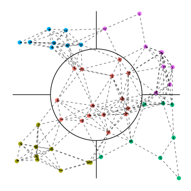
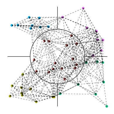
(a) $r=0.5$.	(b) $r=0.75$.

Figure 1: A $50$-node network with two connection radiuses. Solid lines show the clusters and dash lines represent the edges in the network.

Due to space limitation, we only provide the numerical results of the impacts of the choices of regularization on accuracy and cost. More detailed numerical studies can be found in the supplementary materials. We compare our MST_s-based $\ell_{1}$ regularization ($\Theta(K)$ penalty terms) to the pairwise $\ell_{1}$ regularization ($O(K^{2})$ penalty tems), which will be referred to as Graph-$\ell_{1}$ regularization in this section. Both models are solved by our proposed generalized ADMM algorithm distributively. In the distributed algorithm, the nodes need to update the local $\mathbf{w}_{i},$ $\bm{\Delta}_{i,l}$ and $\mathbf{z}_{i,l}$ in each iteration. Clearly, the amount of data being transmitted grows as the graph becomes denser. We simulate a $50$-node network and each node contains $50$ samples. We adjust the network denseness by changing the connection radius $r$. Two setting are compared: $r=0.50$ and $r=0.75$ (see Figure 1 (a) – (b)). We compare the accuracy and costs of the two models with $100$ simulations. The MSEs and the estimated cluster number $\hat{S}$ are used for measuring accuracy. We set the baseline to be the average computation time and the average communication cost for the MST_s $\ell_{1}$ model under $r=0.50$. The boxplots for the accuracy, the computation time ratios, and the communication cost ratios are shown in Figure 2. We can see that our method outperforms in all aspects: Our method improves the MSE at least $21\%$, while reducing at least $38\%$ computation time and $55\%$ communication cost.

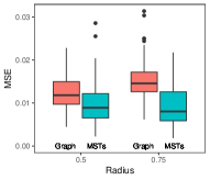
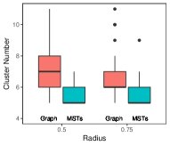
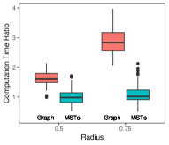
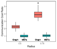
Figure 2: The boxplots of MSEs of $\hat{\mathbf{w}}$, the estimated group numbers $\hat{S}$, the computation time ratio and the communication cost ratio of the graph $\ell_{1}$ regularization and MST_s $\ell_{1}$ regularization.

8 Conclusion

In this work, we considered the problem of distributively learning the regression coefficient heterogeneity over networks. We developed a new minimum spanning tree based adaptive fused-lasso model and a low-complexity distributed generalized ADMM algorithm to solve the problem. We investigated the theoretical properties of both the model consistency and the algorithm convergence. We showed that our model enjoys the oracle properties (i.e., selection consistency and asymptotic normality) and our distributed optimization algorithm has a linear convergence rate. An interesting future topic is to generalize our framework to a more general class of regression problems including generalized linear model and semi-parameteric linear model.

References

- [Ando and Zhang(2007)] Rie K Ando and Tong Zhang. Learning on graph with laplacian regularization. In Advances in neural information processing systems, pages 25–32, 2007.
- [Boyd et al.(2011)Boyd, Parikh, Chu, Peleato, and Eckstein] S. Boyd, N. Parikh, E. Chu, B. Peleato, and J. Eckstein. Distributed optimization and statistical learning via the alternating direction method of multipliers. Foundations and Trends in Machine Learning, 3(1):1 – 122, 2011.
- [Chaganty and Liang(2013)] Arun Tejasvi Chaganty and Percy Liang. Spectral experts for estimating mixtures of linear regressions. In International Conference on Machine Learning, pages 1040–1048, 2013.
- [Chow et al.(2016)Chow, Shi, Wu, and Yin] Yat-Tin Chow, Wei Shi, Tianyu Wu, and Wotao Yin. Expander graph and communication-efficient decentralized optimization. In 2016 50th Asilomar Conference on Signals, Systems and Computers, pages 1715–1720. IEEE, 2016.
- [Deng and Yin(2016)] Wei Deng and Wotao Yin. On the global and linear convergence of the generalized alternating direction method of multipliers. Journal of Scientific Computing, 66(3):889–916, 2016.
- [Eisen et al.(2017)Eisen, Mokhtari, and Ribeiro] Mark Eisen, Aryan Mokhtari, and Alejandro Ribeiro. Decentralized quasi-newton methods. IEEE Transactions on Signal Processing, 65(10):2613–2628, 2017.
- [Fan and Li(2001)] Jianqing Fan and Runze Li. Variable selection via nonconcave penalized likelihood and its oracle properties. Journal of the American statistical Association, 96(456):1348–1360, 2001.
- [Gallager et al.(1983)Gallager, Humblet, and Spira] Robert G. Gallager, Pierre A. Humblet, and Philip M. Spira. A distributed algorithm for minimum-weight spanning trees. ACM Transactions on Programming Languages and systems (TOPLAS), 5(1):66–77, 1983.
- [Hallac et al.(2015)Hallac, Leskovec, and Boyd] David Hallac, Jure Leskovec, and Stephen Boyd. Network lasso: Clustering and optimization in large graphs. In Proceedings of the 21th ACM SIGKDD international conference on knowledge discovery and data mining, pages 387–396. ACM, 2015.
- [Hastie and Tibshirani(1996)] Trevor Hastie and Robert Tibshirani. Discriminant analysis by gaussian mixtures. Journal of the Royal Statistical Society: Series B (Methodological), 58(1):155–176, 1996.
- [Jiang et al.(2018)Jiang, Mukherjee, and Sarkar] Zhanhong Jiang, Kushal Mukherjee, and Soumik Sarkar. On consensus-disagreement tradeoff in distributed optimization. In 2018 Annual American Control Conference (ACC), pages 571–576. IEEE, 2018.
- [Ke et al.(2015)Ke, Fan, and Wu] Zheng Tracy Ke, Jianqing Fan, and Yichao Wu. Homogeneity pursuit. Journal of the American Statistical Association, 110(509):175–194, 2015.
- [Konecny et al.(2015)Konecny, McMahan, and Ramage] Jakub Konecny, Brendan McMahan, and Daniel Ramage. Federated optimization: Distributed optimization beyond the datacenter. arXiv preprint arXiv:1511.03575, 2015.
- [Lee et al.(2015)Lee, Zhu, and Toscas] D-J Lee, Z Zhu, and P Toscas. Spatio-temporal functional data analysis for wireless sensor networks data. Environmetrics, 26(5):354–362, 2015.
- [Li and Sang(2018)] Furong Li and Huiyan Sang. Spatial homogeneity pursuit of regression coefficients for large datasets. Journal of the American Statistical Association, (just-accepted):1–37, 2018.
- [Ma and Huang(2017)] Shujie Ma and Jian Huang. A concave pairwise fusion approach to subgroup analysis. Journal of the American Statistical Association, 112(517):410–423, 2017.
- [Ma et al.(2018)Ma, Huang, and Zhang] Shujie Ma, Jian Huang, and Zhiwei Zhang. Exploration of heterogeneous treatment effects via concave fusion. arXiv preprint arXiv:1607.03717, 2018.
- [Nedic and Ozdaglar(2009)] Angelia Nedic and Asuman Ozdaglar. Distributed subgradient methods for multi-agent optimization. IEEE Transactions on Automatic Control, 54(1):48, 2009.
- [Rohe et al.(2011)Rohe, Chatterjee, Yu, et al.] Karl Rohe, Sourav Chatterjee, Bin Yu, et al. Spectral clustering and the high-dimensional stochastic blockmodel. The Annals of Statistics, 39(4):1878–1915, 2011.
- [Shen and He(2015)] Juan Shen and Xuming He. Inference for subgroup analysis with a structured logistic-normal mixture model. Journal of the American Statistical Association, 110(509):303–312, 2015.
- [Shi et al.(2014)Shi, Ling, Yuan, Wu, and Yin] Wei Shi, Qing Ling, Kun Yuan, Gang Wu, and Wotao Yin. On the linear convergence of the admm in decentralized consensus optimization. IEEE Transactions on Signal Processing, 62(7):1750–1761, 2014.
- [Tang and Song(2016)] Lu Tang and Peter XK Song. Fused lasso approach in regression coefficients clustering: learning parameter heterogeneity in data integration. The Journal of Machine Learning Research, 17(1):3915–3937, 2016.
- [Wahlberg et al.(2012)Wahlberg, Boyd, Annergren, and Wang] Bo Wahlberg, Stephen Boyd, Mariette Annergren, and Yang Wang. An admm algorithm for a class of total variation regularized estimation problems. IFAC Proceedings Volumes, 45(16):83–88, 2012.
- [Wang et al.(2018)Wang, Wang, Kolar, and Srebro] Weiran Wang, Jialei Wang, Mladen Kolar, and Nathan Srebro. Distributed stochastic multi-task learning with graph regularization. arXiv preprint arXiv:1802.03830, 2018.
- [Yuan et al.(2016)Yuan, Ling, and Yin] Kun Yuan, Qing Ling, and Wotao Yin. On the convergence of decentralized gradient descent. SIAM Journal on Optimization, 26(3):1835–1854, 2016.
- [Zhu(2017)] Yunzhang Zhu. An augmented admm algorithm with application to the generalized lasso problem. Journal of Computational and Graphical Statistics, 26(1):195–204, 2017.