Distributed estimation of the inverse Hessian by
determinantal averaging

Abstract

In distributed optimization and distributed numerical linear algebra, we often encounter an inversion bias: if we want to compute a quantity that depends on the inverse of a sum of distributed matrices, then the sum of the inverses does not equal the inverse of the sum. An example of this occurs in distributed Newton’s method, where we wish to compute (or implicitly work with) the inverse Hessian multiplied by the gradient. In this case, locally computed estimates are biased, and so taking a uniform average will not recover the correct solution. To address this, we propose determinantal averaging, a new approach for correcting the inversion bias. This approach involves reweighting the local estimates of the Newton’s step proportionally to the determinant of the local Hessian estimate, and then averaging them together to obtain an improved global estimate. This method provides the first known distributed Newton step that is asymptotically consistent, i.e., it recovers the exact step in the limit as the number of distributed partitions grows to infinity. To show this, we develop new expectation identities and moment bounds for the determinant and adjugate of a random matrix. Determinantal averaging can be applied not only to Newton’s method, but to computing any quantity that is a linear tranformation of a matrix inverse, e.g., taking a trace of the inverse covariance matrix, which is used in data uncertainty quantification.

1 Introduction

Many problems in machine learning and optimization require that we produce an accurate estimate of a square matrix $\mathbf{H}$ (such as the Hessian of a loss function or a sample covariance), while having access to many copies of some unbiased estimator of $\mathbf{H}$, i.e., a random matrix $\widehat{\mathbf{H}}$ such that $\mathbb{E}[\widehat{\mathbf{H}}]=\mathbf{H}$. In these cases, taking a uniform average of those independent copies provides a natural strategy for boosting the estimation accuracy, essentially by making use of the law of large numbers: $\frac{1}{m}\sum_{t=1}^{m}\widehat{\mathbf{H}}_{t}\rightarrow\mathbf{H}$. For many other problems, however, we are more interested in the inverse (Hessian/covariance) matrix $\mathbf{H}^{-1}$, and it is necessary or desirable to work with $\widehat{\mathbf{H}}^{-1}$ as the estimator. Here, a naïve averaging approach has certain fundamental limitations (described in more detail below). The basic reason for this is that $\mathbb{E}[\widehat{\mathbf{H}}^{-1}]\neq\mathbf{H}^{-1}$, i.e., that there is what may be called an inversion bias.

In this paper, we propose a method to address this inversion bias challenge. The method uses a weighted average, where the weights are carefully chosen to compensate for and correct the bias. Our motivation comes from distributed Newton’s method (explained shortly), where combining independent estimates of the inverse Hessian is desired, but our method is more generally applicable, and so we first state our key ideas in a more general context.

Theorem 1

Let $s_{i}$ be independent random variables and $\mathbf{Z}_{i}$ be fixed square rank-$1$ matrices. If  $\widehat{\mathbf{H}}=\sum_{i}s_{i}\mathbf{Z}_{i}$ is invertible almost surely, then the inverse of the matrix $\mathbf{H}=\mathbb{E}[\widehat{\mathbf{H}}]$ can be expressed as:

$$\mathbf{H}^{-1}=\frac{\mathbb{E}\big{[}\!\det(\widehat{\mathbf{H}})\widehat{\mathbf{H}}^{-1}\big{]}}{\mathbb{E}\big{[}\!\det(\widehat{\mathbf{H}})\big{]}}.$$

To demonstrate the implications of Theorem 1, suppose that our goal is to estimate $F(\mathbf{H}^{-1})$ for some linear function $F$. For example, in the case of Newton’s method $F(\mathbf{H}^{-1})=\mathbf{H}^{-1}\mathbf{g}$, where $\mathbf{g}$ is the gradient and $\mathbf{H}$ is the Hessian. Another example would be $F(\mathbf{H}^{-1})=\mathrm{tr}(\mathbf{H}^{-1})$, where $\mathbf{H}$ is the covariance matrix of a dataset and $\mathrm{tr}(\cdot)$ is the matrix trace, which is useful for uncertainty quantification. For these and other cases, consider the following estimation of $F(\mathbf{H}^{-1})$, which takes an average of the individual estimates $F(\widehat{\mathbf{H}}_{t}^{-1})$, each weighted by the determinant of $\widehat{\mathbf{H}}_{t}$, i.e.,

$$\textbf{Determinantal Averaging:}\quad\hat{F}_{m}=\frac{\sum_{t=1}^{m}a_{t}F(\widehat{\mathbf{H}}_{t}^{-1})}{\sum_{t=1}^{m}a_{t}},\qquad a_{t}=\det(\widehat{\mathbf{H}}_{t}).$$

By applying the law of large numbers (separately to the numerator and the denominator), Theorem 1 easily implies that if $\widehat{\mathbf{H}}_{1},\dots,\widehat{\mathbf{H}}_{m}$ are i.i.d. copies of $\widehat{\mathbf{H}}$ then this determinantal averaging estimator is asymptotically consistent, i.e., $\hat{F}_{m}\rightarrow F(\mathbf{H}^{-1})$, almost surely. This determinantal averaging estimator is particularly useful when problem constraints do not allow us to compute $F\big{(}(\frac{1}{m}\sum_{t}\widehat{\mathbf{H}}_{t})^{-1}\big{)}$, e.g., when the matrices are distributed and not easily combined.

To establish finite sample convergence guarantees for estimators obtained via determinantal averaging, we establish the following matrix concentration result. We state it separately since it is technically interesting and since its proof requires novel bounds for the higher moments of the determinant of a random matrix, which is likely to be of independent interest. Below and throughout the paper, $C$ denotes an absolute constant and “$\preceq$” is the Löwner order on positive semi-definite (psd) matrices.

Theorem 2

Let $\widehat{\mathbf{H}}=\frac{1}{k}\sum_{i=1}^{n}b_{i}\mathbf{Z}_{i}\,+\mathbf{B}$ and $\mathbf{H}=\mathbb{E}[\widehat{\mathbf{H}}]$, where $\mathbf{B}$ is a positive definite $d\times d$ matrix and $b_{i}$ are i.i.d. $\mathrm{Bernoulli}(\frac{k}{n})$. Moreover, assume that all $\mathbf{Z}_{i}$ are psd, $d\times d$ and rank-$1$. If $k\geq C\frac{\mu d^{2}}{\eta^{2}}\log^{3}\!\frac{d}{\delta}$  for  $\eta\in(0,1)$  and  $\mu=\max_{i}\|\mathbf{Z}_{i}\mathbf{H}^{-1}\|/d$, then

$$\Big{(}1-\frac{\eta}{\sqrt{m}}\Big{)}\cdot\mathbf{H}^{-1}\preceq\frac{\sum_{t=1}^{m}a_{t}\widehat{\mathbf{H}}_{t}^{-1}}{\sum_{t=1}^{m}a_{t}}\preceq\Big{(}1+\frac{\eta}{\sqrt{m}}\Big{)}\cdot\mathbf{H}^{-1}\quad\text{with probability }\geq 1-\delta,$$

where $\widehat{\mathbf{H}}_{1},\dots,\widehat{\mathbf{H}}_{m}\overset{\textnormal{i.i.d.}}{\sim}\widehat{\mathbf{H}}$ and $a_{t}=\det(\widehat{\mathbf{H}}_{t})$.

1.1 Distributed Newton’s method

To illustrate how determinantal averaging can be useful in the context of distributed optimization, consider the task of batch minimization of a convex loss over vectors $\mathbf{w}\in\mathbb{R}^{d}$, defined as follows:

$$\mathcal{L}(\mathbf{w})\stackrel{{\scriptstyle\textit{\tiny{def}}}}{{=}}\frac{1}{n}\sum_{i=1}^{n}\ell_{i}(\mathbf{w}^{\scriptscriptstyle{\top}}\mathbf{x}_{i})\ +\frac{\lambda}{2}\|\mathbf{w}\|^{2},$$ (1)

where $\lambda>0$, and $\ell_{i}$ are convex, twice differentiable and smooth. Given a vector $\mathbf{w}$, Newton’s method dictates that the correct way to move towards the optimum is to perform an update $\widetilde{\mathbf{w}}=\mathbf{w}-\mathbf{p}$, with $\mathbf{p}=\nabla^{-2}\!\mathcal{L}(\mathbf{w})\,\nabla\!\mathcal{L}(\mathbf{w})$, where $\nabla^{-2}\!\mathcal{L}(\mathbf{w})=(\nabla^{2}\mathcal{L}(\mathbf{w}))^{-1}$ denotes the inverse Hessian of $\mathcal{L}$ at $\mathbf{w}$. Here, the Hessian and gradient are:

$$\nabla^{2}\!\mathcal{L}(\mathbf{w})=\frac{1}{n}\sum_{i}\ell_{i}^{\prime\prime}(\mathbf{w}^{\scriptscriptstyle{\top}}\mathbf{x}_{i})\,\mathbf{x}_{i}\mathbf{x}_{i}^{\scriptscriptstyle{\top}}\,+\lambda\mathbf{I},\quad\text{and}\quad\nabla\!\mathcal{L}(\mathbf{w})=\frac{1}{n}\sum_{i}\ell_{i}^{\prime}(\mathbf{w}^{\scriptscriptstyle{\top}}\mathbf{x}_{i})\,\mathbf{x}_{i}\ +\lambda\mathbf{w}.$$

For our distributed Newton application, we study a distributed computational model, where a single machine has access to a subsampled version of $\mathcal{L}$ with sample size parameter $k\ll n$:

$$\widehat{\mathcal{L}}(\mathbf{w})\stackrel{{\scriptstyle\textit{\tiny{def}}}}{{=}}\frac{1}{k}\sum_{i=1}^{n}b_{i}\ell_{i}(\mathbf{w}^{\scriptscriptstyle{\top}}\mathbf{x}_{i})\ +\frac{\lambda}{2}\|\mathbf{w}\|^{2},\quad\text{where}\quad b_{i}\sim\mathrm{Bernoulli}\big{(}k/n\big{)}.$$ (2)

Note that $\widehat{\mathcal{L}}$ accesses on average $k$ loss components $\ell_{i}$ ($k$ is the expected local sample size), and moreover, $\mathbb{E}\big{[}\widehat{\mathcal{L}}(\mathbf{w})\big{]}=\mathcal{L}(\mathbf{w})$ for any $\mathbf{w}$. The goal is to compute local estimates of the Newton’s step $\mathbf{p}$ in a communication-efficient manner (i.e., by only sending $O(d)$ parameters from/to a single machine), then combine them into a better global estimate. The gradient has size $O(d)$ so it can be computed exactly within this communication budget (e.g., via map-reduce), however the Hessian has to be approximated locally by each machine. Note that other computational models can be considered, such as those where the global gradient is not computed (and local gradients are used instead).

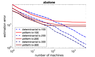
Figure 1: Newton step estimation error versus number of machines, averaged over 100 runs (shading is standard error) for a libsvm dataset [CL11]. More plots in Appendix C.

Under the constraints described above, the most natural strategy is to use directly the Hessian of the locally subsampled loss $\widehat{\mathcal{L}}$ (see, e.g., GIANT [WRKXM18]), resulting in the approximate Newton step $\widehat{\mathbf{p}}=\nabla^{-2}\!\widehat{\mathcal{L}}(\mathbf{w})\,\nabla\!\mathcal{L}(\mathbf{w})$. Suppose that we independently construct $m$ i.i.d. copies of this estimate: $\widehat{\mathbf{p}}_{1},\dots,\widehat{\mathbf{p}}_{m}$ (here, $m$ is the number of machines). Then, for sufficiently large $m$, taking a simple average of the estimates will stop converging to $\mathbf{p}$ because of the inversion bias: $\frac{1}{m}\sum_{t=1}^{m}\widehat{\mathbf{p}}_{t}\rightarrow\mathbb{E}\big{[}\widehat{\mathbf{p}}\big{]}\neq\mathbf{p}$. Figure 1 shows this by plotting the estimation error (in Euclidean distance) of the averaged Newton step estimators, when the weights are uniform and determinantal (for more details and plots, see Appendix C).

The only way to reduce the estimation error beyond a certain point is to increase the local sample size $k$ (thereby reducing the inversion bias), which raises the computational cost per machine. Determinantal averaging corrects the inversion bias so that estimation error can always be decreased by adding more machines without increasing the local sample size. From the preceding discussion we can easily show that determinantal averaging leads to an asymptotically consistent estimator. This is a corollary of Theorem 1, as proven in Section 2.

Corollary 3

Let $\{\widehat{\mathcal{L}}_{t}\}_{t=1}^{\infty}$ be i.i.d. samples of (2) and define $a_{t}=\det\!\big{(}\nabla^{2}\!\widehat{\mathcal{L}}_{t}(\mathbf{w})\big{)}$. Then:

$$\frac{\sum_{t=1}^{m}a_{t}\,\widehat{\mathbf{p}}_{t}}{\sum_{t=1}^{m}a_{t}}\ \overset{\text{a.s.}}{\underset{m\rightarrow\infty}{\longrightarrow}}\ \mathbf{p},\quad\text{where}\quad\widehat{\mathbf{p}}_{t}=\nabla^{-2}\!\widehat{\mathcal{L}}_{t}(\mathbf{w})\,\nabla\!\mathcal{L}(\mathbf{w})\ \text{ and }\ \mathbf{p}=\nabla^{-2}\!\mathcal{L}(\mathbf{w})\,\nabla\!\mathcal{L}(\mathbf{w}).$$

The (unnormalized) determinantal weights can be computed locally in the same time as it takes to compute the Newton estimates so they do not add to the overall cost of the procedure. While this result is only an asymptotic statement, it holds with virtually no assumptions on the loss function (other than twice-differentiability) or the expected local sample size $k$. However, with some additional assumptions we will now establish a convergence guarantee with a finite number of machines $m$ by bounding the estimation error for the determinantal averaging estimator of the Newton step.

In the next result, we use Mahalanobis distance, denoted $\|\mathbf{v}\|_{\mathbf{M}}=\sqrt{\mathbf{v}^{\scriptscriptstyle{\top}}\mathbf{M}\mathbf{v}}$, to measure the error of the Newton step estimate (i.e., the deviation from optimum $\mathbf{p}$), with $\mathbf{M}$ chosen as the Hessian of $\mathcal{L}$. This choice is motivated by standard convergence analysis of Newton’s method, discussed next. This is a corollary of Theorem 2, as explained in Section 3.

Corollary 4

For any $\delta,\eta\!\in\!(0,1)$ if expected local sample size satisfies $k\geq C\eta^{-2}\mu d^{2}\log^{3}\!\frac{d}{\delta}$ then

$$\bigg{\|}\,\frac{\sum_{t=1}^{m}a_{t}\,\widehat{\mathbf{p}}_{t}}{\sum_{t=1}^{m}a_{t}}\,-\,\mathbf{p}\,\bigg{\|}_{\nabla^{2}\!\mathcal{L}(\mathbf{w})}\!\!\leq\frac{\eta}{\sqrt{m}}\cdot\big{\|}\,\mathbf{p}\,\big{\|}_{\nabla^{2}\!\mathcal{L}(\mathbf{w})}\quad\text{with probability }\geq 1-\delta,$$

where $\mu=\frac{1}{d}\max_{i}\ell_{i}^{\prime\prime}(\mathbf{w}^{\scriptscriptstyle{\top}}\!\mathbf{x}_{i})\|\mathbf{x}_{i}\|^{2}_{\nabla^{-2}\!\mathcal{L}(\mathbf{w})}$, and $a_{t}$, $\widehat{\mathbf{p}}_{t}$ and $\mathbf{p}$ are defined as in Corollary 3.

We next establish how this error bound impacts the convergence guarantees offered by Newton’s method. Note that under our assumptions $\mathcal{L}$ is strongly convex so there is a unique minimizer $\mathbf{w}^{*}=\operatorname*{\mathop{\mathrm{argmin}}}_{\mathbf{w}}\mathcal{L}(\mathbf{w})$. We ask how the distance from optimum, $\|\mathbf{w}-\mathbf{w}^{*}\|$, changes after we make an update $\widetilde{\mathbf{w}}=\mathbf{w}-\widehat{\mathbf{p}}$. For this, we have to assume that the Hessian matrix is $L$-Lipschitz as a function of $\mathbf{w}$. After this standard assumption, a classical analysis of the Newton’s method reveals that Corollary 4 implies the following Corollary 6 (proof in Appendix B).

Assumption 5

The Hessian is $L$-Lipschitz: $\|\nabla^{2}\!\mathcal{L}(\mathbf{w})-\nabla^{2}\!\mathcal{L}(\widetilde{\mathbf{w}})\|\leq L\,\|\mathbf{w}-\widetilde{\mathbf{w}}\|$ for any $\mathbf{w},\widetilde{\mathbf{w}}\in\mathbb{R}^{d}$.

Corollary 6

For any $\delta,\eta\!\in\!(0,1)$ if expected local sample size satisfies $k\geq C\eta^{-2}\mu d^{2}\log^{3}\!\frac{d}{\delta}$ then under Assumption 5 it holds with probability at least $1-\delta$ that

$$\big{\|}\widetilde{\mathbf{w}}-\mathbf{w}^{*}\big{\|}\leq\max\Big{\{}\frac{\eta}{\sqrt{m}}\sqrt{\kappa}\,\big{\|}\mathbf{w}-\mathbf{w}^{*}\big{\|},\ \ \frac{2L}{\lambda_{\min}}\,\big{\|}\mathbf{w}-\mathbf{w}^{*}\big{\|}^{2}\Big{\}}\quad\text{ for }\ \widetilde{\mathbf{w}}=\mathbf{w}-\frac{\sum_{t=1}^{m}a_{t}\,\widehat{\mathbf{p}}_{t}}{\sum_{t=1}^{m}a_{t}},$$

where $C$, $\mu$, $a_{t}$ and $\widehat{\mathbf{p}}_{t}$ are defined as in Corollaries 3 and 4, while $\kappa$ and $\lambda_{\min}$ are the condition number and smallest eigenvalue of $\nabla^{2}\!\mathcal{L}(\mathbf{w})$, respectively.

The bound is a maximum of a linear and a quadratic convergence term. As $m$ goes to infinity and/or $\eta$ goes to $0$ the approximation coefficient $\alpha=\frac{\eta}{\sqrt{m}}$ in the linear term disappears and we obtain exact Newton’s method, which exhibits quadratic convergence (at least locally around $\mathbf{w}^{*}$). However, decreasing $\eta$ means increasing $k$ and with it the average computational cost per machine. Thus, to preserve the quadratic convergence while maintaining a computational budget per machine, as the optimization progresses we have to increase the number of machines $m$ while keeping $k$ fixed. This is only possible when we correct for the inversion bias, which is done by determinantal averaging.

1.2 Distributed data uncertainty quantification

Here, we consider another example of when computing a compressed linear representation of the inverse matrix is important. Let $\mathbf{X}$ be an $n\times d$ matrix where the rows $\mathbf{x}_{i}^{\scriptscriptstyle{\top}}$ represent samples drawn from a population for statistical analysis. The sample covariance matrix $\mathbf{\Sigma}=\frac{1}{n}\mathbf{X}^{\scriptscriptstyle{\top}}\mathbf{X}$ holds the information about the relations between the features. Assuming that $\mathbf{\Sigma}$ is invertible, the matrix $\mathbf{\Sigma}^{-1}$, also known as the precision matrix, is often used to establish a degree of confidence we have in the data collection [KBCG13]. The diagonal elements of $\mathbf{\Sigma}^{-1}$ are particularly useful since they hold the variance information of each individual feature. Thus, efficiently estimating either the entire diagonal, its trace, or some subset of its entries is of practical interest [Ste97, WLK⁺16, BCF09]. We consider the distributed setting where data is separately stored in batches and each local covariance is modeled as:

$$\widehat{\mathbf{\Sigma}}=\frac{1}{k}\sum_{i=1}^{n}b_{i}\mathbf{x}_{i}\mathbf{x}_{i}^{\scriptscriptstyle{\top}},\quad\text{where}\quad b_{i}\sim\mathrm{Bernoulli}(k/n).$$

For each of the local covariances $\widehat{\mathbf{\Sigma}}_{1},\dots,\widehat{\mathbf{\Sigma}}_{m}$, we compute its compressed uncertainty information: $F\big{(}(\widehat{\mathbf{\Sigma}}_{t}+\frac{\eta}{\sqrt{m}}\mathbf{I})^{-1}\big{)}$, where we added a small amount of ridge to ensure invertibility. Here, $F(\cdot)$ may for example denote the trace or the vector of diagonal entries. We arrive at the following asymptotically consistent estimator for $F(\mathbf{\Sigma}^{-1})$:

$$\hat{F}_{m}=\frac{\sum_{t=1}^{m}a_{t,m}F\big{(}(\widehat{\mathbf{\Sigma}}_{t}+\frac{\eta}{\sqrt{m}}\mathbf{I})^{-1}\big{)}}{\sum_{t=1}^{m}a_{t,m}},\quad\mbox{where}\quad a_{t,m}=\det\!\big{(}\widehat{\mathbf{\Sigma}}_{t}+\tfrac{\eta}{\sqrt{m}}\mathbf{I}\big{)}.$$

Note that the ridge term $\frac{\eta}{\sqrt{m}}\mathbf{I}$ decays to zero as $m$ goes to infinity, which is why $\hat{F}_{m}\rightarrow F(\mathbf{\Sigma}^{-1})$. Even though this limit holds for any local sample size $k$, in practice we should choose $k$ sufficiently large so that $\widehat{\mathbf{\Sigma}}$ is well-conditioned. In particular, Theorem 2 implies that if $k\geq 2C\eta^{-2}\mu d^{2}\log^{3}\!\frac{d}{\delta}$, where $\mu=\frac{1}{d}\max_{i}\|\mathbf{x}_{i}\|_{\mathbf{\Sigma}^{-1}}^{2}$, then for $F(\cdot)=\mathrm{tr}(\cdot)$ we have $|\hat{F}_{m}-\mathrm{tr}(\mathbf{\Sigma}^{-1})|\leq\frac{\eta}{\sqrt{m}}\cdot\mathrm{tr}(\mathbf{\Sigma}^{-1})$ w.p. $1-\delta$.

1.3 Related work

Many works have considered averaging strategies for combining distributed estimates, particularly in the context of statistical learning and optimization. This research is particularly important in federated learning [KBRR16, KBY⁺16], where data are spread out accross a large network of devices with small local storage and severely constrained communication bandwidth. Using averaging to combine local estimates has been studied in a number of learning settings [MMS⁺09, MHM10] as well as for first-order stochastic optimization [ZWLS10, AD11]. For example, [ZDW13] examine the effectiveness of simple uniform averaging of emprical risk minimizers and also propose a bootstrapping technique to reduce the bias.

More recently, distributed averaging methods gained considerable attention in the context of second-order optimization, where the Hessian inversion bias is of direct concern. [SSZ14] propose a distributed approximate Newton-type method (DANE) which under certain assumptions exhibits low bias. This was later extended and improved upon by [ZL15, RKR⁺16]. The GIANT method of [WRKXM18] most closely follows our setup from Section 1.1, providing non-trivial guarantees for uniform averaging of the Newton step estimates $\widehat{\mathbf{p}}_{t}$ (except they use with-replacement uniform sampling, whereas we use without-replacement, but that is typically a negligible difference). A related analysis of this approach is provided in the context of ridge regression by [WGM17]. Finally, [ABH17] propose a different estimate of the Hessian inverse by using the Neuman series expansion, and use it to construct Newton step estimates which exhibit low bias when the Hessian is sufficiently well-conditioned.

Our approach is related to recent developments in determinantal subsampling techniques (e.g. volume sampling), which have been shown to correct the inversion bias in the context of least squares regression [DW17, DWH19]. However, despite recent progress [DW18, DWH18], volume sampling is still far too computationally expensive to be feasible for distributed optimization. Indeed, often uniform sampling is the only practical choice in this context.

With the exception of the expensive volume sampling-based methods, all of the approaches discussed above, even under favorable conditions, use biased estimates of the desired solution (e.g., the exact Newton step). Thus, when the number of machines grows sufficiently large, with fixed local sample size, the averaging no longer provides any improvement. This is in contrast to our determinantal averaging, which converges exactly to the desired solution and requires no expensive subsampling. Therefore, it can scale with an arbitrarily large number of machines.

2 Expectation identities for determinants and adjugates

In this section, we prove Theorem 1 and Corollary 3, establishing that determinantal averaging is asymptotically consistent. To achieve this, we establish a lemma involving two expectation identities.

For a square $n\times n$ matrix $\mathbf{A}$, we use $\operatorname{\mathrm{adj}}(\mathbf{A})$ to denote its adjugate, defined as an $n\times n$ matrix whose $(i,j)$th entry is $(-1)^{i+j}\det(\mathbf{A}_{-j,-i})$, where $\mathbf{A}_{-j,-i}$ denotes $\mathbf{A}$ without $j$th row and $i$th column. The adjugate matrix provides a key connection between the inverse and the determinant because for any invertible matrix $\mathbf{A}$, we have $\operatorname{\mathrm{adj}}(\mathbf{A})=\det(\mathbf{A})\mathbf{A}^{-1}$. In the following lemma, we will also use a formula called Sylvester’s theorem, relating the adjugate and the determinant: $\det(\mathbf{A}+\mathbf{u}\mathbf{v}^{\scriptscriptstyle{\top}})=\det(\mathbf{A})+\mathbf{v}^{\scriptscriptstyle{\top}}\!\operatorname{\mathrm{adj}}(\mathbf{A})\mathbf{u}$.

Lemma 7

For $\mathbf{A}=\sum_{i}s_{i}\mathbf{Z}_{i}$, where $s_{i}$ are independently random and $\mathbf{Z}_{i}$ are square and rank-$1$,

$$\mathrm{(a)}\ \ \mathbb{E}\big{[}\det(\mathbf{A})\big{]}=\det\!\big{(}\mathbb{E}[\mathbf{A}]\big{)}\quad\text{and}\quad\mathrm{(b)}\ \ \mathbb{E}\big{[}\operatorname{\mathrm{adj}}(\mathbf{A})\big{]}=\operatorname{\mathrm{adj}}\!\big{(}\mathbb{E}[\mathbf{A}]\big{)}.$$

Proof  We use induction over the number of components in the sum. If there is only one component, i.e., $\mathbf{A}=s\mathbf{Z}$, then $\det(\mathbf{A})=0$ a.s. unless $\mathbf{Z}$ is $1\!\times\!1$, in which case (a) is trivial, and $(b)$ follows similarly. Now, suppose we showed the hypothesis when the number of components is $n$ and let $\mathbf{A}=\sum_{i=1}^{n+1}s_{i}\mathbf{Z}_{i}$. Setting $\mathbf{Z}_{n+1}=\mathbf{u}\mathbf{v}^{\scriptscriptstyle{\top}}$, we have:

$$\mathbb{E}\big{[}\det(\mathbf{A})\big{]} =\mathbb{E}\bigg{[}\det\!\Big{(}\sum_{i=1}^{n}s_{i}\mathbf{Z}_{i}+s_{n+1}\mathbf{u}\mathbf{v}^{\scriptscriptstyle{\top}}\Big{)}\bigg{]}$$

(Sylvester’s Theorem) $$=\mathbb{E}\bigg{[}\det\!\Big{(}\sum_{i=1}^{n}s_{i}\mathbf{Z}_{i}\Big{)}+s_{n+1}\mathbf{v}^{\scriptscriptstyle{\top}}\!\operatorname{\mathrm{adj}}\!\Big{(}\sum_{i=1}^{n}s_{i}\mathbf{Z}_{i}\Big{)}\mathbf{u}\bigg{]}$$

(inductive hypothesis) $$=\det\!\bigg{(}\mathbb{E}\Big{[}\sum_{i=1}^{n}s_{i}\mathbf{Z}_{i}\Big{]}\bigg{)}+\mathbb{E}[s_{n+1}]\,\mathbf{v}^{\scriptscriptstyle{\top}}\!\operatorname{\mathrm{adj}}\!\bigg{(}\mathbb{E}\Big{[}\sum_{i=1}^{n}s_{i}\mathbf{Z}_{i}\Big{]}\bigg{)}\mathbf{u}$$

(Sylvester’s Theorem) $$=\det\!\bigg{(}\mathbb{E}\Big{[}\sum_{i=1}^{n}s_{i}\mathbf{Z}_{i}\Big{]}+\mathbb{E}[s_{n+1}]\,\mathbf{u}\mathbf{v}^{\scriptscriptstyle{\top}}\bigg{)}\ =\ \det\!\big{(}\mathbb{E}[\mathbf{A}]\big{)},$$

showing (a). Finally, (b) follows by applying (a) to each entry $\operatorname{\mathrm{adj}}(\mathbf{A})_{ij}=(-1)^{i+j}\det(\mathbf{A}_{-j,-i})$.  
Similar expectation identities for the determinant have been given before [vdV65, DWH19, Der18]. None of them, however, apply to the random matrix $\mathbf{A}$ as defined in Lemma 7, or even to the special case we use for analyzing distributed Newton’s method. Also, our proof method is quite different, and somewhat simpler, than those used in prior work. To our knowledge, the extension of determinantal expectation to the adjugate matrix has not previously been pointed out.

We next prove Theorem 1 and Corollary 3 as consequences of Lemma 7.

Proof of Theorem 1  When $\mathbf{A}$ is invertible, its adjugate is given by $\operatorname{\mathrm{adj}}(\mathbf{A})=\det(\mathbf{A})\mathbf{A}^{-1}$, so the lemma implies that

$$\mathbb{E}\big{[}\!\det(\mathbf{A})\big{]}\big{(}\mathbb{E}[\mathbf{A}]\big{)}^{-1}=\det\!\big{(}\mathbb{E}[\mathbf{A}]\big{)}\big{(}\mathbb{E}[\mathbf{A}]\big{)}^{-1}=\operatorname{\mathrm{adj}}(\mathbb{E}[\mathbf{A}])=\mathbb{E}\big{[}\!\operatorname{\mathrm{adj}}(\mathbf{A})\big{]}=\mathbb{E}\big{[}\!\det(\mathbf{A})\mathbf{A}^{-1}\big{]},$$

from which Theorem 1 follows immediately.  

Proof of Corollary 3  The subsampled Hessian matrix used in Corollary 3 can be written as:

$$\nabla^{2}\!\widehat{\mathcal{L}}(\mathbf{w})=\frac{1}{k}\sum_{i}b_{i}\ell_{i}^{\prime\prime}(\mathbf{w}^{\scriptscriptstyle{\top}}\mathbf{x}_{i})\,\mathbf{x}_{i}\mathbf{x}_{i}^{\scriptscriptstyle{\top}}\,+\lambda\sum_{i=1}^{d}\mathbf{e}_{i}\mathbf{e}_{i}^{\scriptscriptstyle{\top}}\,\stackrel{{\scriptstyle\textit{\tiny{def}}}}{{=}}\,\widehat{\mathbf{H}},$$

so, letting $\widehat{\mathbf{H}}_{t}=\nabla^{2}\!\widehat{\mathcal{L}}_{t}(\mathbf{w})$, Corollary 3 follows from Theorem 1 and the law of large numbers:

$$\frac{\sum_{t=1}^{m}a_{t}\,\widehat{\mathbf{p}}_{t}}{\sum_{t=1}^{m}a_{t}} =\frac{\frac{1}{m}\sum_{t=1}^{m}\det\!\big{(}\widehat{\mathbf{H}}_{t}\big{)}\widehat{\mathbf{H}}_{t}^{-1}\nabla\!\mathcal{L}(\mathbf{w})}{\frac{1}{m}\sum_{t=1}^{m}\det\!\big{(}\widehat{\mathbf{H}}_{t}\big{)}}\underset{m\rightarrow\infty}{\longrightarrow}\frac{\mathbb{E}\big{[}\!\det(\widehat{\mathbf{H}})\widehat{\mathbf{H}}^{-1}\big{]}}{\mathbb{E}\big{[}\!\det(\widehat{\mathbf{H}})\big{]}}\nabla\!\mathcal{L}(\mathbf{w})=\nabla^{-2}\!\mathcal{L}(\mathbf{w})\,\nabla\!\mathcal{L}(\mathbf{w}),$$

which concludes the proof.  

3 Finite-sample convergence analysis

In this section, we prove Theorem 2 and Corollary 4, establishing that determinantal averaging exhibits a $1/\sqrt{m}$ convergence rate, where $m$ is the number of sampled matrices (or the number of machines in distributed Newton’s method). For this, we need a tool from random matrix theory.

Lemma 8 (Matrix Bernstein [Tro12])

Consider a finite sequence $\{\mathbf{X}_{i}\}$ of independent, random, self-adjoint matrices with dimension d such that $\mathbb{E}[\mathbf{X}_{i}]=\mathbf{0}$ and $\lambda_{\max}(\mathbf{X}_{i})\leq R$ almost surely. If the sequence satisfies $\big{\|}\!\sum_{i}\mathbb{E}[\mathbf{X}_{i}^{2}]\big{\|}\leq\sigma^{2}$, then the following inequality holds for all $x\geq 0$:

$$\Pr\!\bigg{(}\lambda_{\max}\Big{(}\sum\nolimits_{i}\mathbf{X}_{i}\Big{)}\geq x\bigg{)}\leq\begin{cases}d\,\mathrm{e}^{-\frac{x^{2}}{4\sigma^{2}}}&\text{for }x\leq\frac{\sigma^{2}}{R};\\ d\,\mathrm{e}^{-\frac{x}{4R}}&\text{for }x\geq\frac{\sigma^{2}}{R}.\end{cases}$$

The key component of our analysis is bounding the moments of the determinant and adjugate of a certain class of random matrices. This has to be done carefully, because higher moments of the determinant grow more rapidly than, e.g., for a sub-gaussian random variable. For this result, we do not require that the individual components $\mathbf{Z}_{i}$ of matrix $\mathbf{A}$ be rank-1, but we impose several additional boundedness assumptions. In the proof below we apply the concentration inequality of Lemma 8 twice: first to the random matrix $\mathbf{A}$ itself, and then also to its trace, which allows finer control over the determinant.

Lemma 9

Let $\mathbf{A}=\frac{1}{\gamma}\sum_{i}b_{i}\mathbf{Z}_{i}\,+\mathbf{B}$, where $b_{i}\sim\mathrm{Bernoulli}(\gamma)$ are independent, whereas $\mathbf{Z}_{i}$ and $\mathbf{B}$ are $d\times d$ psd matrices such that $\|\mathbf{Z}_{i}\|\leq\epsilon$ for all $i$ and $\mathbb{E}[\mathbf{A}]=\mathbf{I}$. If $\gamma\geq 8\epsilon d\eta^{-2}(p+\ln d)$ for $0<\eta\leq 0.25$ and $p\geq 2$, then

$$\mathrm{(a)}\ \ \mathbb{E}\Big{[}\big{|}\det(\mathbf{A})-1\big{|}^{p}\Big{]}^{\frac{1}{p}}\leq 5\eta\quad\text{and}\quad\mathrm{(b)}\ \ \mathbb{E}\Big{[}\big{\|}\operatorname{\mathrm{adj}}(\mathbf{A})-\mathbf{I}\big{\|}^{p}\Big{]}^{\frac{1}{p}}\leq 9\eta.$$

Proof  We start by proving (a). Let $X=\det(\mathbf{A})-1$ and denote $\mathbf{1}_{[a,b]}$ as the indicator variable of the event that $X\in[a,b]$. Since $\det(\mathbf{A})\geq 0$, we have:

$$\mathbb{E}\big{[}|X|^{p}\big{]} =\mathbb{E}\big{[}(-X)^{p}\cdot\mathbf{1}_{[-1,0]}\big{]}+\mathbb{E}\big{[}X^{p}\cdot\mathbf{1}_{[0,\infty]}\big{]}$$

$$\leq\eta^{p}\ +\ \int_{\eta}^{1}px^{p-1}\Pr(-X\geq x)dx\ +\ \int_{0}^{\infty}px^{p-1}\Pr(X\geq x)dx.$$ (3)

Thus it suffices to bound the two integrals. We will start with the first one. Let $\mathbf{X}_{i}=(1-\frac{b_{i}}{\gamma})\mathbf{Z}_{i}$. We use the matrix Bernstein inequality to control the extreme eigenvalues of the matrix $\mathbf{I}-\mathbf{A}=\sum_{i}\mathbf{X}_{i}$ (note that matrix $\mathbf{B}$ cancels out because $\mathbf{I}=\mathbb{E}[\mathbf{A}]=\sum_{i}\mathbf{Z}_{i}+\mathbf{B}$). To do this, observe that $\|\mathbf{X}_{i}\|\leq\epsilon/\gamma$ and, moreover, $\mathbb{E}\big{[}(1-\frac{b_{i}}{\gamma})^{2}\big{]}=\frac{1}{\gamma}-1\leq\frac{1}{\gamma}$, so:

$$\Big{\|}\sum_{i}\mathbb{E}[\mathbf{X}_{i}^{2}]\Big{\|} =\Big{\|}\sum_{i}\mathbb{E}\big{[}(1-\tfrac{b_{i}}{\gamma})^{2}\big{]}\mathbf{Z}_{i}^{2}\Big{\|}\leq\frac{1}{\gamma}\cdot\Big{\|}\sum_{i}\mathbf{Z}_{i}^{2}\Big{\|}\leq\frac{\epsilon}{\gamma}\cdot\Big{\|}\sum_{i}\mathbf{Z}_{i}\Big{\|}\leq\frac{\epsilon}{\gamma}.$$

Thus, applying Lemma 8 we conclude that for any $z\in\big{[}\frac{\eta}{\sqrt{2d}},1\big{]}$:

$$\Pr\!\Big{(}\|\mathbf{I}-\mathbf{A}\|\geq z\Big{)}\leq 2d\,\mathrm{e}^{-\frac{z^{2}\gamma}{4\epsilon}}\leq 2\mathrm{e}^{\ln(d)-z^{2}\frac{2d}{\eta^{2}}(p+\ln d)}\leq 2\mathrm{e}^{-z^{2}\frac{2dp}{\eta^{2}}}.$$ (4)

Conditioning on the high-probability event given by (4) leads to the lower bound $\det(\mathbf{A})\geq(1-z)^{d}$ which is very loose. To improve on it, we use the following inequality, where $\delta_{1},\dots,\delta_{d}$ denote the eigenvalues of $\mathbf{I}-\mathbf{A}$:

$$\det(\mathbf{A})\mathrm{e}^{\mathrm{tr}(\mathbf{I}-\mathbf{A})}=\prod_{i}(1-\delta_{i})\mathrm{e}^{\delta_{i}}\geq\prod_{i}(1-\delta_{i})(1+\delta_{i})=\prod_{i}(1-\delta_{i}^{2}).$$

Thus we obtain a tighter bound when $\det(\mathbf{A})$ is multiplied by $\mathrm{e}^{\mathrm{tr}(\mathbf{I}-\mathbf{A})}$, and now it suffices to upper bound the latter. This is a simple application of the scalar Bernstein’s inequality (Lemma 8 with $d=1$) for the random variables $X_{i}=\mathrm{tr}(\mathbf{X}_{i})\leq\epsilon/\gamma\leq\frac{\eta^{2}}{8dp}$, which satisfy $\sum_{i}\mathbb{E}[X_{i}^{2}]\leq\frac{\epsilon}{\gamma}\,\mathrm{tr}\big{(}\sum_{i}\mathbf{Z}_{i}\big{)}\leq\frac{\epsilon d}{\gamma}\leq\frac{\eta^{2}}{8p}$. Thus the scalar Bernstein’s inequality states that

$$\max\Big{\{}\Pr\!\big{(}\mathrm{tr}(\mathbf{A}-\mathbf{I})\geq y\big{)},\ \ \Pr\!\big{(}\mathrm{tr}(\mathbf{A}-\mathbf{I})\leq-y\big{)}\Big{\}}\ \leq\ \begin{cases}\mathrm{e}^{-y^{2}\frac{2p}{\eta^{2}}}&\text{for }y\leq d;\\ \mathrm{e}^{-y\frac{2dp}{\eta^{2}}}&\text{for }y\geq d.\end{cases}$$ (5)

Setting $y=\frac{x}{2}$ and $z=\sqrt{\!\frac{x}{2d}}$ and taking a union bound over the appropriate high-probability events given by (4) and (5), we conclude that for any $x\in[\eta,1]$:

$$\det(\mathbf{A})\geq(1-z^{2})^{d}\exp\big{(}\mathrm{tr}(\mathbf{A}-\mathbf{I})\big{)}\geq\big{(}1-\tfrac{x}{2}\big{)}\mathrm{e}^{-\frac{x}{2}}\geq 1-x,\quad\text{with prob. }1-3\mathrm{e}^{-x^{2}\frac{p}{2\eta^{2}}}.$$

Thus, for $X=\det(\mathbf{A})-1$ and $x\in[\eta,1]$ we obtain that $\Pr(-X\geq x)\leq 3\mathrm{e}^{-x^{2}\!\frac{p}{2\eta^{2}}}$, and consequently,

$$\int_{\eta}^{1}\!\!px^{p-1}\,\Pr\!\big{(}-X\geq x\big{)}dx \ \leq\ 3p\int_{\eta}^{1}\!\!x^{p-1}\,\mathrm{e}^{-x^{2}\!\frac{p}{2\eta^{2}}}dx\leq 3p\,\sqrt{\pi\tfrac{2\eta^{2}}{p}}\cdot\int_{-\infty}^{\infty}\!\!|x|^{p-1}\,\frac{\mathrm{e}^{-x^{2}\!\frac{p}{2\eta^{2}}}}{\sqrt{2\pi\eta^{2}/p}}dx$$

$$\leq 3\sqrt{2\pi\eta^{2}p}\cdot\big{(}\tfrac{\eta^{2}}{p}\,p\big{)}^{\frac{p-1}{2}}\ =\ 3\sqrt{2\pi p}\cdot\eta^{p}.$$

We now move on to bounding the remaining integral from (3). Since determinant is the product of eigenvalues, we have $\det(\mathbf{A})=\det(\mathbf{I}+\mathbf{A}-\mathbf{I})\leq\mathrm{e}^{\mathrm{tr}(\mathbf{A}-\mathbf{I})}$, so we can use the Bernstein bound of (5) w.r.t. $\mathbf{A}-\mathbf{I}$. It follows that:

$$\int_{0}^{\infty}\!\!px^{p-1}\Pr(X\geq x)dx \leq\int_{0}^{\infty}\!\!px^{p-1}\Pr\big{(}\mathrm{e}^{\mathrm{tr}(\mathbf{A}-\mathbf{I})}\geq 1+x\big{)}dx$$

$$\leq\int_{0}^{\mathrm{e}^{d}-1}\!\!px^{p-1}\mathrm{e}^{-\ln^{2}(1+x)\frac{2p}{\eta^{2}}}dx\ +\ \int_{\mathrm{e}^{d}-1}^{\infty}\!\!px^{p-1}\mathrm{e}^{-\ln(1+x)\frac{2dp}{\eta^{2}}}dx$$

$$\leq\int_{0}^{\mathrm{e}-1}\!\!px^{p-1}\mathrm{e}^{-\ln^{2}(1+x)\frac{2p}{\eta^{2}}}dx\ +\ \int_{\mathrm{e}-1}^{\infty}\!\!px^{p-1}\mathrm{e}^{-\ln(1+x)\frac{2p}{\eta^{2}}}dx,$$

because $\ln^{2}(1+x)\geq\ln(1+x)$ for $x\geq\mathrm{e}-1$. Note that $\ln^{2}(1+x)\geq x^{2}/4$ for $x\in[0,\mathrm{e}-1]$, so

$$\int_{0}^{\mathrm{e}-1}\!\!px^{p-1}\mathrm{e}^{-\ln^{2}(1+x)\frac{2p}{\eta^{2}}}dx \leq\int_{0}^{\mathrm{e}-1}\!\!px^{p-1}\mathrm{e}^{-x^{2}\!\frac{p}{2\eta^{2}}}dx\leq\sqrt{2\pi p}\cdot\eta^{p}.$$

In the interval $x\in[\mathrm{e}-1,\infty]$, we have:

$$\int_{\mathrm{e}-1}^{\infty}\!\!px^{p-1}\mathrm{e}^{-\ln(1+x)\frac{2p}{\eta^{2}}}dx =p\int_{\mathrm{e}-1}^{\infty}\!\!\mathrm{e}^{(p-1)\ln(x)-\ln(1+x)\frac{2p}{\eta^{2}}}dx\leq p\int_{\mathrm{e}-1}^{\infty}\!\!\mathrm{e}^{-\ln(1+x)\frac{p}{\eta^{2}}}dx$$

$$\leq p\int_{1}^{\infty}\!\!\big{(}\tfrac{1}{1+x}\big{)}^{\frac{p}{\eta^{2}}}dx=\frac{p}{\frac{p}{\eta^{2}}-1}\big{(}\tfrac{1}{2}\big{)}^{\frac{p}{\eta^{2}}-1}\leq p\cdot\Big{(}\big{(}\tfrac{1}{2}\big{)}^{\frac{1}{\eta^{2}}}\Big{)}^{p}\ \leq\ p\cdot\big{(}\eta^{2}\big{)}^{p},$$

where the last inequality follows because $(\frac{1}{2})^{\frac{1}{\eta^{2}}}\leq\eta^{2}$. Noting that $(1+4\sqrt{2\pi p}+p)^{\frac{1}{p}}\leq 5$ for any $p\geq 2$ concludes the proof of (a). The proof of (b), given in Appendix A, follows similarly as above because for any positive definite $\mathbf{A}$ we have $\frac{\det(\mathbf{A})}{\lambda_{\max}(\mathbf{A})}\cdot\mathbf{I}\preceq\operatorname{\mathrm{adj}}(\mathbf{A})\preceq\frac{\det(\mathbf{A})}{\lambda_{\min}}\cdot\mathbf{I}$.  
Having obtained bounds on the higher moments, we can now convert them to convergence with high probability for the average of determinants and the adjugates. Since determinant is a scalar variable, this follows by using standard arguments. On the other hand, for the adjugate matrix we require a somewhat less standard matrix extension of the Khintchine/Rosenthal inequalities (see Appendix A).

Corollary 10

There is $C>0$ s.t. for $\mathbf{A}$ as in Lemma 9 with all $\mathbf{Z}_{i}$ rank-$1$ and $\gamma\geq C\epsilon d\eta^{-2}\log^{3}\!\frac{d}{\delta}$,

$$(a)\ \Pr\!\bigg{(}\Big{|}\frac{1}{m}\sum_{t=1}^{m}\det(\mathbf{A}_{t})-1\Big{|}\geq\!\frac{\eta}{\sqrt{m}}\bigg{)}\leq\delta\quad\text{and}\quad(b)\ \Pr\!\bigg{(}\Big{\|}\frac{1}{m}\sum_{t=1}^{m}\operatorname{\mathrm{adj}}(\mathbf{A}_{t})-\mathbf{I}\Big{\|}\geq\!\frac{\eta}{\sqrt{m}}\bigg{)}\leq\delta,$$

where $\mathbf{A}_{1},\dots,\mathbf{A}_{m}$ are independent copies of $\mathbf{A}$.

We are ready to show the convergence rate of determinantal averaging, which follows essentially by upper/lower bounding the enumerator and denominator separately, using Corollary 10.

Proof of Theorem 2  We will apply Corollary 10 to the matrices $\mathbf{A}_{t}=\mathbf{H}^{-\frac{1}{2}}\widehat{\mathbf{H}}_{t}\mathbf{H}^{-\frac{1}{2}}$. Note that $\mathbf{A}_{t}=\frac{n}{k}\sum_{i}b_{i}\widetilde{\mathbf{Z}}_{i}+\lambda\mathbf{H}^{-1}$, where each $\widetilde{\mathbf{Z}}_{i}=\frac{1}{n}\mathbf{H}^{-\frac{1}{2}}\mathbf{Z}_{i}\mathbf{H}^{-\frac{1}{2}}$ satisfies $\|\widetilde{\mathbf{Z}}_{i}\|\leq\mu\cdot d/n$. Therefore, Corollary 10 guarantees that for $\frac{k}{n}\geq C\frac{\mu d}{n}d\eta^{-2}\log^{3}\!\frac{d}{\delta}$, with probability $1-\delta$ the following average of determinants is concentrated around 1:

$$Z\ \stackrel{{\scriptstyle\textit{\tiny{def}}}}{{=}}\ \frac{1}{m}\sum_{t}\frac{\det(\widehat{\mathbf{H}}_{t})}{\det(\mathbf{H})}\ =\ \frac{1}{m}\sum_{t}\det\!\big{(}\mathbf{H}^{-\frac{1}{2}}\widehat{\mathbf{H}}_{t}\mathbf{H}^{-\frac{1}{2}}\big{)}\ \in\ [1-\alpha,1+\alpha]\quad\text{ for }\alpha=\frac{\eta}{\sqrt{m}},$$

along with a corresponding bound for the adjugate matrices. We obtain that with probability $1-2\delta$,

$$\bigg{\|}\,\frac{\sum_{t=1}^{m}\operatorname{\mathrm{adj}}(\mathbf{A}_{t})}{\sum_{t=1}^{m}\det(\mathbf{A}_{t})}-\mathbf{I}\,\bigg{\|} \leq\Big{\|}\frac{1}{m}\sum_{t}\operatorname{\mathrm{adj}}\!\big{(}\mathbf{A}_{t}\big{)}-Z\,\mathbf{I}\Big{\|}\,/Z$$

(Corollary 10a) $$\leq\frac{1}{1-\alpha}\Big{\|}\frac{1}{m}\sum_{t}\operatorname{\mathrm{adj}}\!\big{(}\mathbf{A}_{t}\big{)}-\mathbf{I}\Big{\|}+\frac{\alpha}{1-\alpha}$$

(Corollary 10b) $$\leq\frac{\alpha}{1-\alpha}+\frac{\alpha}{1-\alpha}.$$

It remains to multiply the above expressions by $\mathbf{H}^{-\frac{1}{2}}$ from both sides to recover the desired estimator:

$$\frac{\sum_{t=1}^{m}\det(\widehat{\mathbf{H}}_{t})\,\widehat{\mathbf{H}}_{t}^{-1}}{\sum_{t=1}^{m}\det(\widehat{\mathbf{H}}_{t})}=\mathbf{H}^{-\frac{1}{2}}\,\frac{\sum_{t=1}^{m}\operatorname{\mathrm{adj}}(\mathbf{A}_{t})}{\sum_{t=1}^{m}\det(\mathbf{A}_{t})}\,\mathbf{H}^{-\frac{1}{2}}\preceq\mathbf{H}^{-\frac{1}{2}}\big{(}1+\tfrac{2\alpha}{1-\alpha}\big{)}\,\mathbf{I}\,\mathbf{H}^{-\frac{1}{2}}=\big{(}1+\tfrac{2\alpha}{1-\alpha}\big{)}\mathbf{H}^{-1},$$

and the lower bound follows identically. Appropriately adjusting the constants concludes the proof.  

As an application of the above result, we show how this allows us to bound the estimation error in distributed Newton’s method, when using determinantal averaging.

Proof of Corollary 4  Follows from Theorem 2 by setting $\mathbf{Z}_{i}=\ell_{i}^{\prime\prime}(\mathbf{w}^{\scriptscriptstyle{\top}}\mathbf{x}_{i})\mathbf{x}_{i}\mathbf{x}_{i}^{\scriptscriptstyle{\top}}$ and $\mathbf{B}=\lambda\mathbf{I}$. Note that the assumptions imply that $\|\mathbf{Z}_{i}\|\leq\mu$, so invoking the theorem and denoting $\mathbf{g}$ as $\nabla\!\mathcal{L}(\mathbf{w})$, with probability $1-\delta$ we have

$$\bigg{\|}\,\frac{\sum_{t=1}^{m}a_{t}\,\widehat{\mathbf{p}}_{t}}{\sum_{t=1}^{m}a_{t}}\,-\,\mathbf{p}\,\bigg{\|}_{\mathbf{H}} =\bigg{\|}\mathbf{H}^{\frac{1}{2}}\bigg{(}\frac{\sum_{t=1}^{m}\det(\widehat{\mathbf{H}}_{t})\,\widehat{\mathbf{H}}_{t}^{-1}}{\sum_{t=1}^{m}\det(\widehat{\mathbf{H}}_{t})}-\mathbf{H}^{-1}\bigg{)}\mathbf{H}^{\frac{1}{2}}\,\mathbf{H}^{-\frac{1}{2}}\mathbf{g}\bigg{\|}$$

$$\leq\bigg{\|}\mathbf{H}^{\frac{1}{2}}\bigg{(}\frac{\sum_{t=1}^{m}\det(\widehat{\mathbf{H}}_{t})\,\widehat{\mathbf{H}}_{t}^{-1}}{\sum_{t=1}^{m}\det(\widehat{\mathbf{H}}_{t})}-\mathbf{H}^{-1}\bigg{)}\mathbf{H}^{\frac{1}{2}}\bigg{\|}\cdot\big{\|}\mathbf{H}^{-\frac{1}{2}}\mathbf{g}\big{\|}$$

(Theorem 2) $$\leq\big{\|}\mathbf{H}^{\frac{1}{2}}\tfrac{\eta}{\sqrt{m}}\mathbf{H}^{-1}\mathbf{H}^{\frac{1}{2}}\big{\|}\cdot\|\mathbf{p}\|_{\mathbf{H}}\ =\ \tfrac{\eta}{\sqrt{m}}\cdot\|\mathbf{p}\|_{\mathbf{H}},$$

which completes the proof of the corollary.  

Acknowledgements

MWM would like to acknowledge ARO, DARPA, NSF and ONR for providing partial support of this work. Also, MWM and MD thank the NSF for funding via the NSF TRIPODS program. Part of this work was done while MD and MWM were visiting the Simons Institute for the Theory of Computing.

Appendix A Omitted proofs from Section 3

In Section 3, we stated Lemma 9 and proved the first part of it (a moment bound for the determinant). Here, we provide the proof of the second part (a moment bound for the adjugate).

Lemma 11 (Lemma 9b restated)

Let $\mathbf{A}=\frac{1}{\gamma}\sum_{i}b_{i}\mathbf{Z}_{i}\,+\mathbf{B}$, where $b_{i}\sim\mathrm{Bernoulli}(\gamma)$ are independent, whereas $\mathbf{Z}_{i}$ and $\mathbf{B}$ are $d\times d$ psd matrices such that $\|\mathbf{Z}_{i}\|\leq\epsilon$ for all $i$ and $\mathbb{E}[\mathbf{A}]=\mathbf{I}$. If $\gamma\geq 8\epsilon d\eta^{-2}(p+\ln d)$ for $0<\eta\leq 0.25$ and $p\geq 2$, then

$$\mathbb{E}\Big{[}\big{\|}\operatorname{\mathrm{adj}}(\mathbf{A})-\mathbf{I}\big{\|}^{p}\Big{]}^{\frac{1}{p}}\leq 9\eta.$$

Proof  Let $\lambda_{\max}$ and $\lambda_{\min}$ denote the largest and smallest eigenvalue of $\operatorname{\mathrm{adj}}(\mathbf{A})$. We have

$$\mathbb{E}\big{[}\|\operatorname{\mathrm{adj}}(\mathbf{A})-\mathbf{I}\|^{p}\big{]} =\int_{0}^{\infty}\!\!\!px^{p-1}\Pr\big{(}\|\operatorname{\mathrm{adj}}(\mathbf{A})-\mathbf{I}\|\geq x\big{)}dx$$

$$\leq\eta^{p}+\int_{\eta}^{\infty}\!\!\!px^{p-1}\!\Big{(}\!\Pr(\lambda_{\max}\geq 1+x)+\Pr(\lambda_{\min}\leq 1-x)\Big{)}dx.$$

We will now bound the two probabilities. Let $\delta_{\max}$ and $\delta_{\min}$ denote the largest and smallest eigenvalue of matrix $\mathbf{A}-\mathbf{I}$. Recall the following concentration bounds implied by Lemma 8 (see the first part of the proof of Lemma 9):

$$\max\Big{\{}\Pr\!\big{(}\mathrm{tr}(\mathbf{A}-\mathbf{I})\geq y\big{)},\ \ \Pr\big{(}\mathrm{tr}(\mathbf{A}-\mathbf{I})\leq-y\big{)}\Big{\}}\ \leq\ \begin{cases}\mathrm{e}^{-y^{2}\frac{2p}{\eta^{2}}}&\text{for }y\in[0,d];\\ \mathrm{e}^{-y\,\frac{2dp}{\eta^{2}}}&\text{for }y\geq d,\end{cases}$$ (6)

$$\max\Big{\{}\Pr\big{(}\delta_{\max}\geq z\big{)},\ \ \Pr\big{(}\delta_{\min}\leq-z\big{)}\Big{\}}\ \leq\ \begin{cases}\mathrm{e}^{-z^{2}\frac{2p}{\eta^{2}}}&\text{ for }z\in[0,\frac{\eta}{\sqrt{2d}}];\\ \mathrm{e}^{-z^{2}\frac{2dp}{\eta^{2}}}&\text{ for }z\in[\frac{\eta}{\sqrt{2d}},1];\\ \mathrm{e}^{-z\frac{2dp}{\eta^{2}}}&\text{ for }z\geq 1.\end{cases}$$ (7)

From the formula $\operatorname{\mathrm{adj}}(\mathbf{A})=\det(\mathbf{A})\mathbf{A}^{-1}$ it follows that $\lambda_{\max}\leq\frac{\det(\mathbf{A})}{1+\delta_{\min}}\leq\frac{\mathrm{e}^{\mathrm{tr}(\mathbf{A}-\mathbf{I})}}{1+\delta_{\min}}$ so we have

$$\Pr\big{(}\lambda_{\max}\!\geq\!1+x\big{)} \leq\Pr\bigg{(}\frac{\mathrm{e}^{\mathrm{tr}(\mathbf{A}-\mathbf{I})}}{1+\delta_{\min}}\geq 1+x\bigg{)}$$

$$=\Pr\Big{(}\mathrm{tr}(\mathbf{A}-\mathbf{I})+\ln\frac{1}{1+\delta_{\min}}\geq\ln(1+x)\Big{)}$$

$$\leq\Pr\Big{(}\mathrm{tr}(\mathbf{A}-\mathbf{I})\geq\frac{2}{3}\cdot\ln(1+x)\Big{)}\ +\ \Pr\Big{(}\ln\frac{1}{1+\delta_{\min}}\geq\frac{1}{3}\cdot\ln(1+x)\Big{)}$$

$$=\Pr\Big{(}\mathrm{tr}(\mathbf{A}-\mathbf{I})\geq\frac{2}{3}\cdot\ln(1+x)\Big{)}\ +\ \Pr\Big{(}\delta_{\min}\leq\frac{1}{(1+x)^{\frac{1}{3}}}-1\Big{)}.$$

$$\leq\begin{cases}\mathrm{e}^{-\ln^{2}\!(1+x)\frac{8p}{9\eta^{2}}}+\mathrm{e}^{-(1-(\frac{1}{1+x})^{\frac{1}{3}})^{2}\frac{2p}{\eta^{2}}}\leq 2\mathrm{e}^{-x^{2}\frac{p}{20\eta^{2}}}&\text{ for }x\in[0,\mathrm{e}\!-\!1],\\ \mathrm{e}^{-\ln(1+x)\frac{4p}{3\eta^{2}}}+\mathrm{e}^{-\frac{1}{16}\frac{2dp}{\eta^{2}}}\qquad\quad\leq 2\mathrm{e}^{-\ln(1+x)\frac{p}{8\eta^{2}}}&\text{ for }x\in[\mathrm{e}\!-\!1,\mathrm{e}^{d}\!-\!1].\end{cases}$$

For $x\geq\mathrm{e}^{d}-1$, since $\lambda_{\max}\leq(1+\delta_{\max})^{d}\leq e^{d\delta_{\max}}$ and $\ln(1+x)\geq d$, we have:

$$\Pr\big{(}\lambda_{\max}\!\geq\!1+x\big{)}\leq\Pr\big{(}\mathrm{e}^{d\delta_{\max}}\!\geq\!1+x\big{)}=\Pr\big{(}\delta_{\max}\!\geq\!\ln(1+x)/d\big{)}\leq\mathrm{e}^{-\ln(1+x)\frac{2p}{\eta^{2}}}.$$

Next, we use the fact that for $\delta=\max\big{\{}|\delta_{\max}|,|\delta_{\min}|\big{\}}$ we have:

$$\lambda_{\min}\geq\frac{\det(\mathbf{A})}{1+\delta_{\max}}\geq\frac{(1-\delta^{2})^{d}}{(1+\delta_{\max})\mathrm{e}^{\mathrm{tr}(\mathbf{I}-\mathbf{A})}}\geq(1-\delta)(1-d\delta^{2})\big{(}1-\mathrm{tr}(\mathbf{I}-\mathbf{A})\big{)},$$

so for $x\in[\eta,1]$ we have:

$$\Pr\big{(}\lambda_{\min}\leq 1-x\big{)} \leq\Pr(\delta\geq x/3)+\Pr(\delta^{2}\geq x/3d)+\Pr\big{(}\mathrm{tr}(\mathbf{I}-\mathbf{A})\geq x/3\big{)}$$

$$\leq 2\mathrm{e}^{-x^{2}\frac{2dp}{9\eta^{2}}}+2\mathrm{e}^{-\frac{x}{3d}\frac{2dp}{\eta^{2}}}+\mathrm{e}^{-x^{2}\frac{2p}{\eta^{2}}}\ \leq\ 5\mathrm{e}^{-x^{2}\frac{2p}{9\eta^{2}}}.$$

Putting everything together we obtain that:

$$\mathbb{E}\big{[}\|\operatorname{\mathrm{adj}}(\mathbf{A})-\mathbf{I}\|^{p}\big{]} \leq\eta^{p}+\int_{\eta}^{\mathrm{e}-1}px^{p-1}\,7\mathrm{e}^{-x^{2}\frac{p}{20\eta^{2}}}\mathrm{d}x+\int_{\mathrm{e}-1}^{\infty}px^{p-1}3\mathrm{e}^{-\ln(1+x)\frac{p}{8\eta^{2}}}\mathrm{d}x$$

$$\leq\eta^{p}+7\sqrt{20\pi p}\,\eta^{p}+\frac{3p}{\frac{p}{16\eta^{2}}-1}\big{(}\tfrac{1}{2}\big{)}^{\frac{p}{16\eta^{2}}-1}$$

$$\leq\eta^{p}+7\sqrt{20\pi p}\,\eta^{p}+6(3\eta)^{p}\ \leq\ (9\eta)^{p},$$

which completes the proof.  

As a consequence of the moment bounds shown in Lemma 9, we establish convergence with high probability for the average of determinants and the adjugates. For the adjugate matrix, we require a matrix variant of the Khintchine/Rosenthal inequalities.

Lemma 12 ([GCT12])

Suppose that $p\geq 2$ and $r=\max\{p,2\log d\}$. Consider a finite sequence $\{\mathbf{X}_{i}\}$ of independent, symmetrically random, self-adjoint matrices with dimension $d\times d$. Then,

$$\mathbb{E}\Big{[}\big{\|}\sum\nolimits_{i}\mathbf{X}_{i}\big{\|}^{p}\Big{]}^{\frac{1}{p}}\leq\sqrt{\mathrm{e}r}\,\Big{\|}\sum\nolimits_{i}\mathbb{E}[\mathbf{X}_{i}^{2}]\Big{\|}^{\frac{1}{2}}+2\mathrm{e}r\,\mathbb{E}\big{[}\!\max\nolimits_{i}\|\mathbf{X}_{i}\|^{p}\big{]}^{\frac{1}{p}}.$$

Corollary 13 (Corollary 10 restated)

There is $C>0$ s.t. for $\mathbf{A}$ as in Lemma 9 with all $\mathbf{Z}_{i}$ rank-$1$ and $\gamma\geq C\epsilon d\eta^{-2}\log^{3}\!\frac{d}{\delta}$,

$$(a)\ \Pr\!\bigg{(}\Big{|}\frac{1}{m}\sum_{t=1}^{m}\det(\mathbf{A}_{t})-1\Big{|}\geq\!\frac{\eta}{\sqrt{m}}\bigg{)}\leq\delta\quad\text{and}\quad(b)\ \Pr\!\bigg{(}\Big{\|}\frac{1}{m}\sum_{t=1}^{m}\operatorname{\mathrm{adj}}(\mathbf{A}_{t})-\mathbf{I}\Big{\|}\geq\!\frac{\eta}{\sqrt{m}}\bigg{)}\leq\delta,$$

where $\mathbf{A}_{1},\dots,\mathbf{A}_{m}$ are independent copies of $\mathbf{A}$.

Proof  Applying Lemma 9 to the matrix $\mathbf{A}$, for appropriate $C$ and any fixed $p\geq 2$, if $\gamma\geq C\epsilon d\sigma^{-2}(p+\ln d)$, then for any $s\in[2,p]$ we have $\mathbb{E}\big{[}\|\operatorname{\mathrm{adj}}(\mathbf{A}_{t})-\mathbf{I}\|^{s}\big{]}\leq\sigma^{s}$. With the additional assumption that $\mathbf{Z}_{i}$’s are rank-$1$, Theorem 7 implies that $\mathbb{E}\big{[}\operatorname{\mathrm{adj}}(\mathbf{A}_{t})\big{]}=\mathbf{I}$, so by a standard symmetrization argument, where $r_{t}$ denote independent Rademacher random variables,

$$\mathbb{E}\bigg{[}\Big{\|}\frac{1}{m}\sum_{t=1}^{m}\operatorname{\mathrm{adj}}(\mathbf{A}_{t})-\mathbf{I}\Big{\|}^{p}\bigg{]}^{\frac{1}{p}} \leq 2\cdot\mathbb{E}\bigg{[}\Big{\|}\sum_{t}\frac{r_{t}}{m}\big{(}\operatorname{\mathrm{adj}}(\mathbf{A}_{t})-\mathbf{I}\big{)}\Big{\|}^{p}\bigg{]}^{\frac{1}{p}}.$$

Applying Lemma 12 to the matrices $\mathbf{X}_{t}=\frac{1}{m}\mathbf{Y}_{t}$, where $\mathbf{Y}_{t}=r_{t}\big{(}\operatorname{\mathrm{adj}}(\mathbf{A}_{t})-\mathbf{I}\big{)}$, we obtain that:

$$\mathbb{E}\bigg{[}\Big{\|}\frac{1}{m}\sum_{t}\mathbf{Y}_{t}\Big{\|}^{p}\bigg{]}^{\frac{1}{p}} \leq\sqrt{\mathrm{e}r}\,\Big{\|}m\cdot\frac{1}{m^{2}}\mathbb{E}[\mathbf{Y}_{t}^{2}]\Big{\|}^{\frac{1}{2}}+\frac{2\mathrm{e}r}{m}\,\mathbb{E}\Big{[}\sum_{i=1}^{m}\|\mathbf{Y}_{i}\|^{p}\Big{]}^{\frac{1}{p}}$$

$$\leq\sqrt{\frac{\mathrm{e}r}{m}}\cdot\mathbb{E}\big{[}\|\mathbf{Y}\|^{2}\big{]}^{\frac{1}{2}}+\frac{2\mathrm{e}r}{m}\Big{(}m\cdot\mathbb{E}\big{[}\|\mathbf{Y}\|^{p}\big{]}\Big{)}^{\frac{1}{p}}$$

$$\leq\bigg{(}\sqrt{\frac{\mathrm{e}r}{m}}+\frac{2\mathrm{e}r}{m^{1-\frac{1}{p}}}\bigg{)}\cdot\sigma\leq C^{\prime}\cdot\frac{p\sigma}{\sqrt{m}},$$

for $p\geq 2\log d$ and $C^{\prime}$ chosen appropriately. Now Markov’s inequality yields:

$$\Pr\bigg{(}\Big{\|}\frac{1}{m}\sum_{t}\operatorname{\mathrm{adj}}(\mathbf{A}_{t})-\mathbf{I}\Big{\|}\geq\alpha\bigg{)} \leq\alpha^{-p}\cdot\mathbb{E}\bigg{[}\Big{\|}\frac{1}{m}\sum_{t}\operatorname{\mathrm{adj}}(\mathbf{A}_{t})-\mathbf{I}\Big{\|}^{p}\bigg{]}\leq\bigg{(}\frac{2C^{\prime}p\sigma}{\alpha\sqrt{m}}\bigg{)}^{p}.$$

Setting $\alpha\!=\!\frac{\eta}{\sqrt{m}}$, $\sigma\!=\!\frac{\eta}{4C^{\prime}p}$ and $p=2\,\lceil\max\{\log d,\log\frac{1}{\delta}\}\rceil$, the above bound becomes $(\frac{1}{2})^{p}\leq\delta$ for $k\geq C^{\prime\prime}\mu d^{2}\eta^{-2}(\log^{3}\!\frac{1}{\delta}+\log^{3}\!d)$. Showing the analogous result for the average of determinants of matrices $\mathbf{A}_{t}$ instead of the adjugates follows identically, except that Lemma 12 can be replaced with the standard scalar Rosenthal’s inequality.  

Appendix B Proof of Newton convergence

Here, we provide a proof of Corollary 6, which describes the convergence guarantees for the approximate Newton step obtained via determinantal averaging. It suffices to show the following lemma.

Lemma 14

Let loss $\mathcal{L}$ be defined as in (1) and assume its Hessian is L-Lipschitz (Assumption 5). If

$$\big{\|}\widehat{\mathbf{p}}-\mathbf{p}^{*}\big{\|}_{\nabla^{2}\!\mathcal{L}(\mathbf{w})}\leq\alpha\,\|\mathbf{p}^{*}\|_{\nabla^{2}\!\mathcal{L}(\mathbf{w})},\quad\text{where}\quad\mathbf{p}^{*}=\nabla^{-2}\!\mathcal{L}(\mathbf{w})\,\nabla\!\mathcal{L}(\mathbf{w}),$$

then the approximate Newton step $\widetilde{\mathbf{w}}=\mathbf{w}-\widehat{\mathbf{p}}$ satisfies:

$$\|\widetilde{\mathbf{w}}-\mathbf{w}^{*}\|\leq\max\Big{\{}\alpha\sqrt{\kappa}\,\|\mathbf{w}-\mathbf{w}^{*}\|,\ \frac{2L}{\sigma_{\min}}\,\|\mathbf{w}-\mathbf{w}^{*}\|^{2}\Big{\}},\quad\text{where }\mathbf{w}^{*}=\operatorname*{\mathop{\mathrm{argmin}}}_{\mathbf{w}}\mathcal{L}(\mathbf{w}),$$

where $\kappa$ and $\sigma_{\min}$ are the condition number and smallest eiganvalue of $\nabla^{2}\!\mathcal{L}(\mathbf{w})$, respectively.

Proof  The lemma essentially follows via the standard analysis of the Newton’s method. For the sake of completeness we will outline the proof following [WRKXM18]. Denoting $\mathbf{H}=\nabla^{2}\!\mathcal{L}(\mathbf{w})$ and $\mathbf{g}=\nabla\!\mathcal{L}(\mathbf{w})$, we define the auxiliary function

$$\phi(\mathbf{p})\stackrel{{\scriptstyle\textit{\tiny{def}}}}{{=}}\mathbf{p}^{\scriptscriptstyle{\top}}\mathbf{H}\mathbf{p}-2\mathbf{p}^{\scriptscriptstyle{\top}}\mathbf{g}.$$

By definition of $\phi(\mathbf{p})$ we have $\phi(\mathbf{p}^{*})=\phi(\mathbf{H}^{-1}\mathbf{g})=-\|\mathbf{p}^{*}\|_{\mathbf{H}}^{2}$. If follows that

$$\phi(\widehat{\mathbf{p}})-\phi(\mathbf{p}^{*}) =\|\mathbf{H}^{\frac{1}{2}}\widehat{\mathbf{p}}\|^{2}-2\mathbf{g}^{\scriptscriptstyle{\top}}\mathbf{H}^{-1}\mathbf{H}\widehat{\mathbf{p}}+\|\mathbf{H}^{\frac{1}{2}}\mathbf{p}^{*}\|^{2}$$

$$=\|\mathbf{H}^{\frac{1}{2}}(\widehat{\mathbf{p}}-\mathbf{p}^{*})\|^{2}=\big{\|}\widehat{\mathbf{p}}-\mathbf{p}^{*}\big{\|}_{\mathbf{H}}^{2}\leq\alpha^{2}\,\|\mathbf{p}^{*}\|_{\mathbf{H}}^{2}=-\alpha^{2}\phi(\mathbf{p}^{*}).$$

We invoke the classical result in local convergence analysis of Newton’s method [NW06], using the statement of Lemma 9 in [WRKXM18].

Lemma 15 ([WRKXM18])

Assume Hessian is L-Lipschitz and that $\widehat{\mathbf{p}}$ satisfies $\phi(\widehat{\mathbf{p}})\leq(1-\alpha^{2})\,\min_{\mathbf{p}}\phi(\mathbf{p})$. Then $\widetilde{\mathbf{w}}=\mathbf{w}-\widehat{\mathbf{p}}$ satisfies

$$\|\widetilde{\mathbf{w}}-\mathbf{w}^{*}\|_{\mathbf{H}}^{2}\leq L\,\|\mathbf{w}-\mathbf{w}^{*}\|^{2}\|\widetilde{\mathbf{w}}-\mathbf{w}^{*}\|+\frac{\alpha^{2}}{1-\alpha^{2}}\|\mathbf{w}-\mathbf{w}^{*}\|_{\mathbf{H}}^{2}.$$

Lemma 15 immediately implies that one of the following two inequalities hold:

$$\|\widetilde{\mathbf{w}}-\mathbf{w}^{*}\| \leq\frac{2L}{\sigma_{\min}(\mathbf{H})}\cdot\|\mathbf{w}-\mathbf{w}^{*}\|^{2},$$

$$\|\widetilde{\mathbf{w}}-\mathbf{w}^{*}\| \leq\frac{\alpha}{\sqrt{1-\alpha^{2}}}\sqrt{\frac{2\lambda_{\max}(\mathbf{H})}{\lambda_{\min}(\mathbf{H})}}\cdot\|\mathbf{w}-\mathbf{w}^{*}\|,$$

which proves Lemma 14.  
Note that Corollary 6 follows immediately by combining Corollary 4 with Lemma 14.

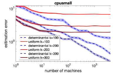
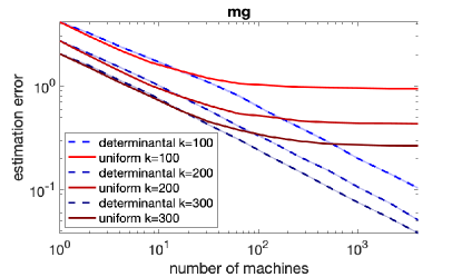
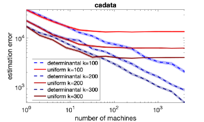
Figure 2: Comparison of the estimation error between determinantal and uniform averaging on four libsvm datasets.

Appendix C Experiments

In this section, we experimentally evaluate the estimation error of determinantal averaging for the Newton’s method (following the setup of Section 1.1), and we compare it against uniform averaging [WRKXM18]. Although there are obvious follow-up directions for empirical and implementational work, here we focus our experiments on demonstrating the existence of the inversion bias with previous methods and how our determinantal averaging solves this problem. We use square loss $\ell_{i}(\mathbf{w}^{\scriptscriptstyle{\top}}\mathbf{x}_{i})=(\mathbf{w}^{\scriptscriptstyle{\top}}\mathbf{x}_{i}-y_{i})^{2}$, where $y_{i}$ are the real-valued labels for a regression problem, and we run the experiments on several benchmark regression datasets from the libsvm repository [CL11]. In this setting, the local Newton estimate computed from the starting vector $\mathbf{w}=\mathbf{0}$ is given by:

$$\widehat{\mathbf{p}}=\bigg{(}\frac{1}{k}\sum_{i=1}^{n}b_{i}\mathbf{x}_{i}\mathbf{x}_{i}^{\scriptscriptstyle{\top}}+\lambda\mathbf{I}\bigg{)}^{-1}\frac{1}{n}\sum_{i=1}^{n}y_{i}\mathbf{x}_{i},\quad\text{where}\quad b_{i}\sim\mathrm{Bernoulli}(k/n).$$

In all of our experiments we set the regularization parameter to $\lambda=\frac{1}{n}$. Let $\widehat{\mathbf{p}}_{1},\dots,\widehat{\mathbf{p}}_{m}\overset{\textnormal{i.i.d.}}{\sim}\widehat{\mathbf{p}}$ be $m$ distributed local estimates and denote $\widehat{\mathbf{H}}_{t}$ as the $t$th local Hessian estimate. The two averaging strategies we compare are:

$$\text{determinantal:}\quad\widehat{\mathbf{p}}_{\det}=\frac{\sum_{t=1}^{m}\det(\widehat{\mathbf{H}}_{t})\,\widehat{\mathbf{p}}_{t}}{\sum_{t=1}^{m}\det(\widehat{\mathbf{H}}_{t})},\qquad\text{uniform:}\quad\widehat{\mathbf{p}}_{\mathrm{uni}}=\frac{1}{m}\sum_{t=1}^{m}\widehat{\mathbf{p}}_{t}.$$

Figure 2 plots the estimation errors $\|\widehat{\mathbf{p}}_{\det}-\mathbf{p}^{*}\|$ and $\|\widehat{\mathbf{p}}_{\mathrm{uni}}-\mathbf{p}^{*}\|$, where $\mathbf{p}^{*}$ is the exact Newton step starting from $\mathbf{w}=\mathbf{0}$, for datasets abalone, cpusmall, mg and cadata [CL11] (for convenience, the plot from Figure 1 in Section 1.1 is repeated here). The reported results are averaged over 100 trials, with shading representing standard error. We consistently observe that for a small number of machines $m$ both methods effectively reduce the estimation error, however after a certain point uniform averaging converges to a biased estimate and the estimation error flattens out. On the other hand, determinantal averaging continues to converge to the optimum as the number of machines keeps growing. We remark that for some datasets determinantal averaging exhibits larger variance than uniform averaging, especially when local sample size is small. Reducing that variance, for example through some form of additional regularization, is a new direction for future work.

References

• [ABH17] Naman Agarwal, Brian Bullins, and Elad Hazan. Second-order stochastic optimization for machine learning in linear time. Journal of Machine Learning Research, 18(116):1–40, 2017.
• [AD11] Alekh Agarwal and John C Duchi. Distributed delayed stochastic optimization. In J. Shawe-Taylor, R. S. Zemel, P. L. Bartlett, F. Pereira, and K. Q. Weinberger, editors, Advances in Neural Information Processing Systems 24, pages 873–881. Curran Associates, Inc., 2011.
• [BCF09] C. Bekas, A. Curioni, and I. Fedulova. Low cost high performance uncertainty quantification. In Proceedings of the 2Nd Workshop on High Performance Computational Finance, WHPCF ’09, pages 8:1–8:8, New York, NY, USA, 2009. ACM.
• [CL11] Chih-Chung Chang and Chih-Jen Lin. LIBSVM: A library for support vector machines. ACM Transactions on Intelligent Systems and Technology, 2:27:1–27:27, 2011.
• [Der18] Michał Dereziński. Fast determinantal point processes via distortion-free intermediate sampling. CoRR, abs/1811.03717, 2018.
• [DW17] Michał Dereziński and Manfred K. Warmuth. Unbiased estimates for linear regression via volume sampling. In Advances in Neural Information Processing Systems 30, pages 3087–3096, Long Beach, CA, USA, December 2017.
• [DW18] Michał Dereziński and Manfred K. Warmuth. Reverse iterative volume sampling for linear regression. Journal of Machine Learning Research, 19(23):1–39, 2018.
• [DWH18] Michał Dereziński, Manfred K. Warmuth, and Daniel Hsu. Leveraged volume sampling for linear regression. In S. Bengio, H. Wallach, H. Larochelle, K. Grauman, N. Cesa-Bianchi, and R. Garnett, editors, Advances in Neural Information Processing Systems 31, pages 2510–2519. Curran Associates, Inc., 2018.
• [DWH19] Michał Dereziński, Manfred K. Warmuth, and Daniel Hsu. Correcting the bias in least squares regression with volume-rescaled sampling. In Proceedings of the 22nd International Conference on Artificial Intelligence and Statistics, 2019.
• [GCT12] Alex Gittens, Richard Y. Chen, and Joel A. Tropp. The masked sample covariance estimator: an analysis using matrix concentration inequalities. Information and Inference: A Journal of the IMA, 1(1):2–20, 05 2012.
• [KBCG13] V. Kalantzis, C. Bekas, A. Curioni, and E. Gallopoulos. Accelerating data uncertainty quantification by solving linear systems with multiple right-hand sides. Numer. Algorithms, 62(4):637–653, April 2013.
• [KBRR16] Jakub Konecný, H. Brendan McMahan, Daniel Ramage, and Peter Richtárik. Federated Optimization: Distributed Machine Learning for On-Device Intelligence. arXiv e-prints, page arXiv:1610.02527, Oct 2016.
• [KBY+16] Jakub Konecný, H. Brendan McMahan, Felix X. Yu, Peter Richtárik, Ananda Theertha Suresh, and Dave Bacon. Federated Learning: Strategies for Improving Communication Efficiency. arXiv e-prints, page arXiv:1610.05492, Oct 2016.
• [MHM10] Ryan McDonald, Keith Hall, and Gideon Mann. Distributed training strategies for the structured perceptron. In Human Language Technologies: The 2010 Annual Conference of the North American Chapter of the Association for Computational Linguistics, HLT ’10, pages 456–464, Stroudsburg, PA, USA, 2010. Association for Computational Linguistics.
• [MMS+09] Ryan Mcdonald, Mehryar Mohri, Nathan Silberman, Dan Walker, and Gideon S. Mann. Efficient large-scale distributed training of conditional maximum entropy models. In Y. Bengio, D. Schuurmans, J. D. Lafferty, C. K. I. Williams, and A. Culotta, editors, Advances in Neural Information Processing Systems 22, pages 1231–1239. Curran Associates, Inc., 2009.
• [NW06] Jorge Nocedal and Stephen J. Wright. Numerical Optimization. Springer, New York, NY, USA, second edition, 2006.
• [RKR+16] Sashank J. Reddi, Jakub Konecný, Peter Richtárik, Barnabás Póczós, and Alex Smola. AIDE: Fast and Communication Efficient Distributed Optimization. arXiv e-prints, page arXiv:1608.06879, Aug 2016.
• [SSZ14] Ohad Shamir, Nati Srebro, and Tong Zhang. Communication-efficient distributed optimization using an approximate Newton-type method. In Eric P. Xing and Tony Jebara, editors, Proceedings of the 31st International Conference on Machine Learning, volume 32 of Proceedings of Machine Learning Research, pages 1000–1008, Bejing, China, 22–24 Jun 2014. PMLR.
• [Ste97] Guy V. G. Stevens. On the inverse of the covariance matrix in portfolio analysis. The Journal of Finance, 53:1821–1827, 1997.
• [Tro12] Joel A. Tropp. User-friendly tail bounds for sums of random matrices. Foundations of Computational Mathematics, 12(4):389–434, August 2012.
• [vdV65] H. Robert van der Vaart. A note on Wilks’ internal scatter. Ann. Math. Statist., 36(4):1308–1312, 08 1965.
• [WGM17] Shusen Wang, Alex Gittens, and Michael W. Mahoney. Sketched ridge regression: Optimization perspective, statistical perspective, and model averaging. In Doina Precup and Yee Whye Teh, editors, Proceedings of the 34th International Conference on Machine Learning, volume 70 of Proceedings of Machine Learning Research, pages 3608–3616, International Convention Centre, Sydney, Australia, 06–11 Aug 2017. PMLR.
• [WLK+16] Lingfei Wu, Jesse Laeuchli, Vassilis Kalantzis, Andreas Stathopoulos, and Efstratios Gallopoulos. Estimating the trace of the matrix inverse by interpolating from the diagonal of an approximate inverse. Journal of Computational Physics, 326:828 – 844, 2016.
• [WRKXM18] Shusen Wang, Farbod Roosta-Khorasani, Peng Xu, and Michael W Mahoney. Giant: Globally improved approximate newton method for distributed optimization. In S. Bengio, H. Wallach, H. Larochelle, K. Grauman, N. Cesa-Bianchi, and R. Garnett, editors, Advances in Neural Information Processing Systems 31, pages 2332–2342. Curran Associates, Inc., 2018.
• [XRKM17] Peng Xu, Farbod Roosta-Khorasani, and Michael Mahoney. Newton-type methods for non-convex optimization under inexact hessian information. Mathematical Programming, August 2017.
• [YXRKM18] Z. Yao, P. Xu, F. Roosta-Khorasani, and M. W. Mahoney. Inexact non-convex Newton-type methods. Technical report, 2018. Preprint: arXiv:1802.06925.
• [ZDW13] Yuchen Zhang, John C. Duchi, and Martin J. Wainwright. Communication-efficient algorithms for statistical optimization. J. Mach. Learn. Res., 14(1):3321–3363, January 2013.
• [ZL15] Yuchen Zhang and Xiao Lin. Disco: Distributed optimization for self-concordant empirical loss. In Francis Bach and David Blei, editors, Proceedings of the 32nd International Conference on Machine Learning, volume 37 of Proceedings of Machine Learning Research, pages 362–370, Lille, France, 07–09 Jul 2015. PMLR.
• [ZWLS10] Martin Zinkevich, Markus Weimer, Lihong Li, and Alex J. Smola. Parallelized stochastic gradient descent. In J. D. Lafferty, C. K. I. Williams, J. Shawe-Taylor, R. S. Zemel, and A. Culotta, editors, Advances in Neural Information Processing Systems 23, pages 2595–2603. Curran Associates, Inc., 2010.