Quantization of graphene plasmons

Abstract

In this article we perform the quantization of graphene plasmons using both a macroscopic approach based on the classical average electromagnetic energy and a quantum hydrodynamic model, in which graphene charge carriers are modeled as a charged fluid. Both models allow to take into account the dispersion of graphenes optical response, with the hydrodynamic model also allowing for the inclusion of non-local effects. Using both methods, the electromagnetic field mode-functions, and the respective frequencies, are determined for two different graphene structures. we show how to quantize graphene plasmons, considering that graphene is a dispersive medium, and taking into account both local and nonlocal descriptions. It is found that the dispersion of graphene’s optical response leads to a non-trivial normalization condition for the mode-functions. The obtained mode-functions are then used to calculate the decay of an emitter, represented by a dipole, via the excitation of graphene surface plasmon-polaritons. The obtained results are compared with the total spontaneous decay rate of the emitter and a near perfect match is found in the relevant spectral range. It is found that non-local effects in graphene’s conductivity, become relevant for the emission rate for small Fermi energies and small distances between the dipole and the graphene sheet.

I Introduction

In many cases, light-matter interaction can be understood in a semi-classical picture, where matter is quantized and the electromagnetic field (EM) is treated classically. This semi-classical approach holds when the number of photons in the field is large or the light source is coherent. On the other hand, in order to understand the properties of a small number of photons the quantization of the EM field is required. Typical phenomena where the quantization of the EM field is necessary involve entanglement, squeezed light, cavity electrodynamics, interaction of photons with nano-mechanical resonators, and near-field radiative effects (Agarwal, 2013).

In near-field radiative effects, plasmonics emerges as a promising candidate to observe quantum effects of the electromagnetic radiation, an example being the Hong-Ou-Mandel interference of plasmons (Heeres et al., 2013). Many other quantum effects in plasmonics exist, such as the survival of entanglement, particle-wave duality, quantum size effects due to reduced dimensions of metallic nanostructures, quantum tunneling of plasmons (which are simultaneously light and matter), and coupling of quantum emitters to surface plasmons (Jacob, 2012; Tame et al., 2013; Martín-Cano et al., 2014; Fakonas et al., 2015; Fitzgerald et al., 2016; Dheur et al., 2016; Bozhevolnyi and Mortensen, 2017; Xu et al., 2018; Fernández-Domínguez et al., 2018).

The exploration of quantum effects in plasmonics in unusual spectral ranges, such as the THz and the mid-IR, has been deterrent by the poor plasmonic response of noble metals in these regions of the electromagnetic spectrum. However, with the emergence of graphene plasmonics (Ju et al., 2011; Fei et al., 2011) the possibility of exploring quantum effects in these yet unexplored spectral regions is a possible prospect. Despite the fact that, at the time of writing, quantum effects involving graphene plasmons remain illusive, the fact that graphene plasmons are characterized by low losses (Fei et al., 2012; Chen et al., 2012; Woessner et al., 2015) boosts the above hope. In addition, graphene plasmons screened by a nearby metal (also called screened or acoustic plasmons) can be confined down to the atomic limit (Alcaraz Iranzo et al., 2018), which certainly opens the prospects of finding rich grounds for quantum plasmonics and nonlocal effects (Lundeberg et al., 2017; Dias et al., 2018). Indeed, the idea of developing quantum optics with plasmons has already a long history (Chang et al., 2006) and quantization of localized plasmons in metallic nanoparticles was recently performed (Alpeggiani and Andreani, 2014; Bordo, 2019).

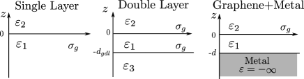
Figure 1: Schematic representation of the three systems considered in this paper: a single graphene layer (left), and graphene double layer (center), and a graphene sheet near a perfect metal. The quantities $\epsilon_{n}$ refer to the dielectric permittivity of the medium $n$ and $\sigma_{g}$ refers to the optical conductivity of graphene.

The development of quantum theory of the electromagnetic field in the presence of dieletric media has a long history and several approaches have been developed (Hopfield, 1958; Alekseev and Nikitin, 1966; Agarwal, 1975a; Huttner and Barnett, 1992; Milonni, 1995; Gruner and Welsch, 1995, 1996; Matloob et al., 1995; Dung et al., 1998; Philbin, 2010; Hanson et al., 2015; Allameh et al., 2016; Sha et al., 2018). These methods are typically based either on the quantization of the macroscopic classic energy(Milonni, 1995), on the classical dyadic Green’s function for the electric field(Gruner and Welsch, 1995) or on the diagonalization of Hopfield-type Hamiltonians(Huttner and Barnett, 1992). The quantization of evanescent EM waves (Carniglia and Mandel, 1971; Carniglia et al., 1972) and of the EM field in the vicinity of a metal (Grossel et al., 1977) have also been considered in the past.

In this paper, we perform the quantization of graphene plasmons, obtaining the plasmonic electromagnetic field mode-functions and, importantly, their normalization, when losses are neglected. These mode-functions are then used to study the interaction of graphene plasmons with nearby quantum emitters and determine, in a very intuitive way, using Fermi’s golden rule the spontaneous decay rate of the emitter due to plasmon emission. Thee quantization of graphene plasmons is performed in two ways: (i) A macroscopic approach, which starts from the classical time-averaged energy of the electromagnetic field in a dielectric (Landau and Lifshitz, 1984; Alekseev and Nikitin, 1966; Agu, 1979; Milonni, 1995). This method allows for the inclusion of dispersion in the optical response of graphene. (ii) A hydrodynamic approach, where graphene charge carriers are described in terms of an electronic fluid, which couples to the eletromagnetic field (Chaves et al., 2017; Fetter, 1973). The hydrodynamic approach allows not only for the inclusion of dispersion, but also for the inclusion of non-local effects in the optical response of graphene.

The paper is organized as follows: in Section II, we present the general macroscopic approach for the quantization of the eletromagnetic field in dispersive, lossless media and a normalization condition for the mode-functions is determined. In Section III, we present the quantum hydrodynamic model or graphene. We will see that when non-local effects are neglected, the result of the macroscopic approach is recovered. In Section IV, the plasmon dispersion relations, mode-functions and mode-function normalization for a single graphene layer and for a graphene-metal structures are obtained. In Section V, we use the quantized plasmon fields to compute the decay rate of a quantum emitter due to the spontaneous emission of plasmons. The plasmon emission rate is compared with the total decay rate of the emitter, which is obtained from the complete dyadic Green’s function for the electric field. The role of non-local response of graphene is analyzed. Finally, we conclude with Section VI, commenting the obtained results and discussing future research paths. A set of appendices detailing the calculations is also presented.

II Macroscopic quantization of the plasmon electromagnetic field

In this section, we will describe how the plasmon fields can be quantized using the macroscopic classical energy of the electromagnetic field in a dispersive, lossless dielectric medium, a method first used in Refs. (Alekseev and Nikitin, 1966; Agu, 1979; Milonni, 1995). For electric and magnetic fields with a harmonic time dependence,

$$\mathbf{E}(\mathbf{r},t) =\mathbf{E}_{\omega}(\mathbf{r})e^{-i\omega t}+\text{c.c.}$$ (1)

$$\mathbf{B}(\mathbf{r},t) =\mathbf{B}_{\omega}(\mathbf{r})e^{-i\omega t}+\text{c.c.}$$ (2)

close to a central frequency $\omega$, the time-averaged classical electromagnetic energy in the presence of a dispersive, lossless dieletric is given by (Landau and Lifshitz, 1984; Ruppin, 2002)

$$U_{\text{EM}}(\omega)=\int d^{3}\mathbf{r}\left(\epsilon_{0}\mathbf{E}_{\omega}^{*}(\mathbf{r})\cdot\frac{\partial}{\partial\omega}\left[\omega\bar{\epsilon}_{r}(\mathbf{r},\omega)\right]\cdot\mathbf{E}_{\omega}(\mathbf{r})\right.\\ \left.+\frac{1}{\mu_{0}}\left|\mathbf{B}_{\omega}\right|^{2}\right),$$ (3)

where $\bar{\epsilon}_{r}(\mathbf{r},\omega)$ is the relative dielectric tensor of the medium, $\epsilon_{0}$ and $\mu_{0}$ are, respectively, vacuum permittivity and permeability. The idea of this method is to take the above equation as the quantum mechanical energy of a EM field eigenmode with frequency $\omega$. We will work in the Weyl gauge, in which the scalar potential is set to zero $\phi=0$, such that the electric and magnetic fields are obtained only from the vector potential $\mathbf{A}$ as

$$\mathbf{E}(\mathbf{r},t) =-\frac{\partial\mathbf{A}(\mathbf{r},t)}{\partial t},$$ (4)

$$\mathbf{B}(\mathbf{r},t) =\nabla\times\mathbf{A}(\mathbf{r},t).$$ (5)

The vector potential is then expanded in modes as

$$\mathbf{A}(\mathbf{r},t)=\sum_{\lambda}\alpha_{\lambda}e^{-i\omega_{\lambda}t}\mathbf{A}_{\lambda}(\mathbf{r})+\text{c.c.},$$ (6)

where $\alpha_{\lambda}$ are amplitudes for the mode $\lambda$, with mode-function $\mathbf{A}_{\lambda}(\mathbf{r})$ and corresponding frequency $\omega_{\lambda}$. The mode-functions and frequencies are determined by solving the non-linear eigenvalue problem

$$\nabla\times\nabla\times\mathbf{A}_{\lambda}(\mathbf{r})=\frac{\omega_{\lambda}^{2}}{c^{2}}\bar{\epsilon}_{r}(\mathbf{r},\omega_{\lambda})\cdot\mathbf{A}_{\lambda}(\mathbf{r}),$$ (7)

with $c$ vacuum’s speed of light, which is just Ampère’s law in the dielectric medium for the mode-function $\mathbf{A}_{\lambda}(\mathbf{r})$. Next, we assume that the total time-averaged energy for the vector potential Eq. (6) is given by

$$U_{\text{EM}}=\sum_{\lambda}U_{\text{EM}}(\omega_{\lambda})\left|\alpha_{\lambda}\right|^{2}.$$ (8)

The quantization of the theory is achieved by promoting the amplitudes $\alpha_{\lambda}$ to quantum mechanical operators

$$\alpha_{\lambda} \rightarrow\sqrt{\frac{\hbar}{2L_{\lambda}\epsilon_{0}\omega_{\lambda}}}\hat{a}_{\lambda},$$ (9)

$$\alpha_{\lambda}^{\dagger} \rightarrow\sqrt{\frac{\hbar}{2L_{\lambda}\epsilon_{0}\omega_{\lambda}}}\hat{a}_{\lambda}^{\dagger},$$ (10)

where $\hat{a}_{\lambda}$ ($\hat{a}_{\lambda}^{\dagger}$) are bosonic annihilation (creation) operators, which obey the usual equal-time commutation relations

$$\left[\hat{a}_{\lambda},\hat{a}_{\lambda^{\prime}}^{\dagger}\right]=\delta_{\lambda,\lambda^{\prime}},$$ (11)

and $L_{\lambda}$ is a mode-length which is determined by demanding that the quantum mechanical Hamiltonian which is obtained from Eq. (8) by performing the replacement of Eqs. (9) and (10),

$$\hat{H}=\sum_{\lambda}\frac{\hbar U(\omega_{\lambda})}{4L_{\lambda}\epsilon_{0}\omega_{\lambda}}\left(\hat{a}_{\lambda}^{\dagger}\hat{a}_{\lambda}+\hat{a}_{\lambda}\hat{a}_{\lambda}^{\dagger}\right),$$ (12)

coincides with the Hamiltonian for a collection of quantum harmonic oscillators

$$\hat{H}=\frac{1}{2}\sum_{\lambda}\hbar\omega_{\lambda}\left(\hat{a}_{\lambda}^{\dagger}\hat{a}_{\lambda}+\hat{a}_{\lambda}\hat{a}_{\lambda}^{\dagger}\right).$$ (13)

Imposing this condition, we have that the mode-length is given by $L_{\lambda}=U(\omega_{\lambda})/\left(2\epsilon_{0}\omega_{\lambda}^{2}\right)$. Using the mode-function equation (7) to write

$$\int d^{3}\mathbf{r}\left|\nabla\times\mathbf{A}_{\lambda}(\mathbf{r})\right|^{2}=\int d^{3}\mathbf{r}\mathbf{A}_{\lambda}^{*}(\mathbf{r})\cdot\nabla\times\nabla\times\mathbf{A}_{\lambda}(\mathbf{r})\\ =\frac{\omega_{\lambda}^{2}}{c^{2}}\int d^{3}\mathbf{r}\mathbf{A}_{\lambda}^{*}(\mathbf{r})\cdot\bar{\epsilon}_{r}(\mathbf{r},\omega_{\lambda})\cdot\mathbf{A}_{\lambda}(\mathbf{r}),$$ (14)

The mode-length can be written as

$$L_{\lambda}=\int d^{3}\mathbf{r}\mathbf{A}_{\lambda}^{*}(\mathbf{r})\cdot\left(\bar{\epsilon}_{r}(\mathbf{r},\omega_{\lambda})+\frac{\omega_{\lambda}}{2}\frac{\partial}{\partial\omega}\bar{\epsilon}_{r}(\mathbf{r},\omega_{\lambda})\right)\cdot\mathbf{A}_{\lambda}(\mathbf{r}).$$ (15)

Notice that in the absence of dispersion, the second term vanishes and $L_{\lambda}$ reduces to the usual norm in the presence of a position dependent dielectric tensor $\bar{\epsilon}_{r}(\mathbf{r},\omega_{\lambda})$.

Although this phenomenological method appears to be unjustified, it has actually been shown to be correct for the case in when the dielectric is modeled by a Lorentz oscillator (Agu, 1979). We will see in the next section, that Eq. 15 remains valid within a quantum hydrodynamic model of graphene, even when non-local effects are included in the optical response. As a matter of fact Eq. (15) for the mode-length remains valid for any linear optical medium (including effects of dispersion, non-locality, inhomogeneity and anisotropy) as long as losses can be neglected (Amorim and Chaves, 2019).

III plasmon quantization within a quantum hydrodynamic model

In this section, we will perform the quantization of graphene surface plasmons employing a hydrodynamic model. The hydrodynamic model treats both the electron gas and the electromagnetic field using a classical picture and provides a simple and elegant way of including non-local effects (Christensen, 2017). Non-local effects are taken into account by including a pressure term in the Boltzmann equation, that arises due to Pauli’s exclusion principle. A detailed derivation of the hydrodynamic model for graphene can be found in (Chaves et al., 2017; Fetter, 1973). To illustrate the method, we choose the simple case of a single graphene sheet located at the plane $z=0$, embedded by a static dielectric medium with relative dielectric constant $\bar{\epsilon}_{d}(\mathbf{r})$.

III.1 Classical hydrodynamic Lagrangean and Hamiltonian

The classical Lagrangean density for the hydrodynamic model of graphene can be written as:

$$\mathcal{L}=\mathcal{L}_{\text{EM}}+\mathcal{L}_{\text{2D hyd}},$$ (16)

where $\mathcal{L}_{\text{EM}}$ is the Lagrangean density of the electromagnetic field and $\mathcal{L}_{\text{2D hyd}}$ describes the electronic fluid of graphene and its coupling to the electromagnetic field. Using once again the Weyl gauge, $\mathcal{L}_{\text{EM}}$ is given by

$$\mathcal{L}_{\text{EM}}=\frac{\epsilon_{0}}{2}\left(\partial_{t}\mathbf{A}\right)\cdot\bar{\epsilon}_{d}\cdot\left(\partial_{t}\mathbf{A}\right)-\frac{1}{2\mu_{0}}\left(\nabla\times\mathbf{A}\right)^{2},$$ (17)

where $\bar{\epsilon}_{d}(\mathbf{r})$ is allowed to be position dependent, but is frequency independent. Within the hydrodynamic model, the electronic fluid of the graphene layer is described by the fluctuation, $n$, of the density around the equilibrium density, $n_{0}$, and the displacement vector $\bm{\upsilon}=\left(\upsilon_{x},\upsilon_{y},0\right)$, which should not be confused with the velocity field. In the Weyl gauge, $\mathcal{L}_{\text{2D fluid}}$ is written as(Fetter, 1973; Chaves et al., 2017)

$$\mathcal{L}_{\text{2D hyd}}=\delta(z)\Biggl{(}\frac{1}{2}n_{0}m\left(\partial_{t}\bm{\upsilon}\right)^{2}+m\beta^{2}n\nabla\cdot\bm{\upsilon}\\ \left.+\frac{m\beta^{2}}{2n_{0}}n^{2}-n_{0}e\partial_{t}\bm{\upsilon}\cdot\mathbf{A}\right),$$ (18)

where the $\delta$-function $\delta(z)$ restricts the electronic fluid to the $z=0$ 2D plane, $m$ is the Drude mass and $\beta$ appears from the relation between the degeneracy pressure and the electronic density and depends on the band dispersion for the carriers (see Ref. (Chaves et al., 2017)). In the approximation of the linear dispersion for graphene electrons, the hydrodynamic parameters are given by (Chaves et al., 2017): $n_{0}=k_{F}^{2}/\pi$, $m=\hbar k_{F}/v_{F}$ and $\beta^{2}=v_{F}^{2}/2$, where $k_{F}$ is the Fermi wavenumber and $v_{F}$ the Fermi velocity of graphene. Equation (18) is the 2D equivalent Lagrangian for the hydrodynamic model presented in (Nakamura, 1983).

Using the Euler-Lagrange equations for Eq. (18) with respect to $\mathbf{A}$, we obtain

$$\nabla\times\mathbf{B}=\frac{1}{c^{2}}\bar{\epsilon}_{d}\partial_{t}\mathbf{E}-\mu_{0}n_{0}e\partial_{t}\boldsymbol{\upsilon}\delta(z),$$ (19)

which is nothing more than Ampère’s law in the presence of a surface current given by

$$\mathbf{J}_{s}^{\text{hyd}}=-en_{0}\partial_{t}\boldsymbol{\upsilon}.$$ (20)

Using the Euler-Lagrange equations for Eq. (18) with respect to the fluid variables $n$ and $\boldsymbol{\upsilon}$, we obtain the continuity and Newton’s second law with a diffusion term, which read respectively

$$n_{0}\nabla\cdot\boldsymbol{\upsilon}+n =0,$$ (21)

$$n_{0}m\partial_{t}^{2}\boldsymbol{\upsilon}+m\beta^{2}\nabla n =-en_{0}\mathbf{E}(z=0),$$ (22)

from which we recognize the fluid electronic surface density

$$\rho_{s}^{\text{hyd}}=-en.$$ (23)

Equations (19)-(22) correspond to the linearized hydrodynamic model for graphene (Chaves et al., 2017) (see also (Lucas and Fong, 2018)).

Notice that Eq. (21) has no dynamics. Therefore, we can use it to eliminate the field $n$, thus obtaining a new Lagrangean density

$$\mathcal{L}^{\prime}=\mathcal{L}_{\text{EM}}+\mathcal{L}_{\text{2D hyd}}^{\prime},$$ (24)

with

$$\mathcal{L}_{\text{2D hyd}}^{\prime}=\delta(z)\Biggl{(}\frac{1}{2}n_{0}m\left(\partial_{t}\bm{\upsilon}\right)^{2}\\ -\frac{1}{2}n_{0}m\beta^{2}\left(\nabla\cdot\bm{\upsilon}\right)^{2}-n_{0}e\partial_{t}\bm{\upsilon}\cdot\mathbf{A}.\Biggr{)}$$ (25)

This new Lagrangean is equivalent to the Eq. (16) as both lead to the same dynamics. Applying the Euler-Lagrange equations to Eq. (24) with respect to $\mathbf{A}$ leads to Eq. (19), while the equation obtained for $\bm{\upsilon}$ reads

$$-m\partial_{t}^{2}\bm{\upsilon}+m\beta^{2}\nabla\left(\nabla\cdot\bm{\upsilon}\right)=e\mathbf{E}(z=0),$$ (26)

which can be obtained by combining Eqs. (21) and (22).

From the Lagrangean density Eq. (24), we define the canonical momenta conjugate to $\mathbf{A}$ and $\bm{\upsilon}$, respectively, as

$$\bm{\Pi} =\frac{\partial\mathcal{L}^{\prime}}{\partial\left(\partial_{t}\mathbf{A}\right)}=\epsilon_{0}\bar{\epsilon}_{d}\partial_{t}\mathbf{A},$$ (27)

$$\bm{\pi} =\frac{\partial\mathcal{L}^{\prime}}{\partial\left(\partial_{t}\bm{\upsilon}\right)}=n_{0}m\partial_{t}\bm{\upsilon}-n_{0}e\mathbf{A}(z=0).$$ (28)

In terms of the variables $\mathbf{A}$, $\bm{\Pi}$, $\bm{\upsilon}$ and $\bm{\pi}$, the classical Hamiltonian obtained from Eq. (24) is given by

$$H=\int d^{3}\mathbf{r}\left(\frac{1}{2\epsilon_{0}}\bm{\Pi}\cdot\bar{\epsilon}_{d}^{-1}\cdot\bm{\Pi}+\frac{1}{2\mu_{0}}\left(\nabla\times\mathbf{A}\right)^{2}\right)\\ +\int d^{2}\mathbf{x}\left(\frac{\left(\bm{\pi}+en_{0}\mathbf{A}(z=0)\right)^{2}}{2n_{0}m}+\frac{1}{2}n_{0}m\beta^{2}\left(\nabla\cdot\bm{\upsilon}\right)^{2}\right).$$ (29)

III.2 Canonical quantization of hydrodynamic model

In order to quantize the classical Hamiltonian Eq. (29), we start by introducing the eigenmodes of the coupled electronic fluid + electromagnetic field. Assuming, we have in-plane translational invariance, we write the vector potential and fluid displacement variables as

$$\mathbf{A}(\mathbf{r},t) =\frac{1}{\sqrt{S}}\sum_{\mathbf{q},\lambda}\alpha_{\mathbf{q},\lambda}(t)e^{i\mathbf{q}\cdot\mathbf{x}}\mathbf{A}_{\mathbf{q},\lambda}(z)+\text{c.c.},$$ (30)

$$\bm{\upsilon}(\mathbf{x},t) =\frac{1}{\sqrt{S}}\sum_{\mathbf{q},\lambda}\alpha_{\mathbf{q},\lambda}(t)e^{i\mathbf{q}\cdot\mathbf{x}}\bm{\upsilon}_{\mathbf{q},\lambda}+\text{c.c.},$$ (31)

where $S$ is the area of the graphene layer, $\alpha_{\mathbf{q},\lambda}(t)=\alpha_{\mathbf{q},\lambda}e^{-i\omega_{\mathbf{q},\lambda}t}$ are mode amplitudes with, $\omega_{\mathbf{q},\lambda}$the mode frequency, and $\mathbf{A}_{\mathbf{q},\lambda}(z)$ and $\bm{\upsilon}_{\mathbf{q},\lambda}$ are mode-functions, which, following from Eqs. (19) and (26), obey the equations

$$\left[\omega_{\mathbf{q},\lambda}^{2}\epsilon_{0}\bar{\epsilon}_{d}(z)-\frac{1}{\mu_{0}}D_{\mathbf{q}}\times D_{\mathbf{q}}\times\right]\mathbf{A}_{\mathbf{q},\lambda}(z)=\\ =-i\omega_{\mathbf{q},\lambda}\delta(z)en_{0}\bm{\upsilon}_{\mathbf{q},\lambda},$$ (32)

$$mn_{0}\left[\omega_{\mathbf{q},\lambda}^{2}-\beta^{2}\mathbf{q}\otimes\mathbf{q}\right]\bm{\upsilon}_{\mathbf{q},\lambda}=i\omega_{\mathbf{q},\lambda}en_{0}\mathbf{A}_{\mathbf{q},\lambda}(0).$$ (33)

where we defined the differential operator $D_{\mathbf{q}}=i\mathbf{q}+\hat{\mathbf{z}}\partial_{z}$.

From Eq. (33), we can write

$$\bm{\upsilon}_{\mathbf{q},\lambda}=\frac{1}{en_{0}}\bar{\sigma}_{g}^{\text{hyd}}\left(\mathbf{q},\omega_{\mathbf{q},\lambda}\right)\cdot\mathbf{A}_{\mathbf{q},\lambda}(0),$$ (34)

where $\bar{\sigma}_{g}^{\text{hyd}}(\mathbf{q},\omega)$ is the conductivity within the hydrodynamic model, which we separate into transverse and longitudinal components as

$$\bar{\sigma}_{g}^{\text{hyd}}(\mathbf{q},\omega) =\sigma_{g,T}^{\text{hyd}}(\mathbf{q},\omega)\left(\bar{1}-\frac{\mathbf{q}\otimes\mathbf{q}}{q^{2}}\right)$$

$$+\sigma_{g,L}^{\text{hyd}}(\mathbf{q},\omega)\frac{\mathbf{q}\otimes\mathbf{q}}{q^{2}},$$ (35)

respectively given by

$$\sigma_{g,T}^{\text{hyd}}(\mathbf{q},\omega) =\frac{e^{2}n_{0}}{m}\frac{i}{\omega},$$ (36)

$$\sigma_{g,L}^{\text{hyd}}(\mathbf{q},\omega) =\frac{e^{2}n_{0}}{m}\frac{i\omega}{\omega^{2}-\beta^{2}q^{2}},$$ (37)

where we identify $D=e^{2}n_{0}/m$ as the Drude weight, which for graphene is given by $D=e^{2}v_{F}k_{F}/\pi$. Notice that in the the limit $\mathbf{q}\rightarrow 0$, $\bar{\sigma}_{g}^{\text{hyd}}(\mathbf{q},\omega)$ reduces to the Drude model. Inserting Eq. (34) into Eq. (32), we obtain

$$D_{\mathbf{q}}\times D_{\mathbf{q}}\times\mathbf{A}_{\mathbf{q},\lambda}(z)=\frac{\omega_{\mathbf{q},\lambda}^{2}}{c^{2}}\bar{\epsilon}_{r}\left(\mathbf{q},z,\omega_{\lambda}\right)\mathbf{A}_{\mathbf{q},\lambda}(z),$$ (38)

with the dieletric function, including screening by graphene electrons, being given by

$$\bar{\epsilon}_{r}\left(\mathbf{q},z,\omega\right)=\bar{\epsilon}_{d}(z)+\frac{i}{\epsilon_{0}\omega}\bar{\sigma}_{g}^{\text{hyd}}\left(\mathbf{q},\omega\right)\delta(z),$$ (39)

in agreement with Eq. (7).

Inserting the expansions Eq. (30) and (31) into Eq. (29), and using the orthogonality properties of the mode-functions $\left(\mathbf{A}_{\mathbf{q},\lambda}(z),\,\bm{\upsilon}_{\mathbf{q},\lambda}\right)$ it is possible to write the Hamiltonian for the hydrodynamic model as (see Appendix (B))

$$H=\frac{1}{2}\sum_{\mathbf{q}\lambda}2\omega_{\mathbf{q},\lambda}^{2}\epsilon_{0}L_{\mathbf{q},\lambda}\alpha_{\mathbf{q},\lambda}^{*}\alpha_{\mathbf{q},\lambda}+\text{c.c},$$ (40)

with the mode-length defined here as

$$L_{\mathbf{q},\lambda} =\int dz\mathbf{A}_{\mathbf{q},\lambda}^{*}(z)\cdot\bar{\epsilon}_{d}(z)\cdot\mathbf{A}_{\mathbf{q},\lambda}(z)+\frac{n_{0}m}{\epsilon_{0}}\bm{\upsilon}_{\mathbf{q},\lambda}^{*}\cdot\bm{\upsilon}_{\mathbf{q},\lambda}$$

$$+\frac{ien_{0}}{2\epsilon_{0}\omega_{\mathbf{q},\lambda}}\left(\mathbf{A}_{\mathbf{q},\lambda}^{*}(0)\cdot\bm{\upsilon}_{\mathbf{q},\lambda}-\bm{\upsilon}_{\mathbf{q},\lambda}^{*}\cdot\mathbf{A}_{\mathbf{q},\lambda}(0)\right).$$ (41)

Promoting the mode amplitudes to quantum mechanical operators as

$$\alpha_{\mathbf{q},\lambda}^{*}(t) \rightarrow\sqrt{\frac{\hbar}{2\epsilon_{0}\omega_{\mathbf{q},\lambda}L_{\mathbf{q},\lambda}}}\hat{a}_{\mathbf{q},\lambda}^{\dagger}(t),$$ (42)

$$\alpha_{\mathbf{q},\lambda}(t) \rightarrow\sqrt{\frac{\hbar}{2\epsilon_{0}\omega_{\mathbf{q},\lambda}L_{\mathbf{q},\lambda}}}\hat{a}_{\mathbf{q},\lambda}(t),$$ (43)

where $\hat{a}_{\mathbf{q},\lambda}^{\dagger}$$\left(\hat{a}_{\mathbf{q},\lambda}\right)$ are creation (annihilation) operators for the plasmon-polaritons, satisfying the usual equal-time commutation relations Eq. (11), the quantum Hamiltonian for the hydrodynamic model becomes

$$\hat{H}=\frac{1}{2}\sum_{\mathbf{q}\lambda}\hbar\omega_{\mathbf{q},\lambda}\left[\hat{a}_{\mathbf{q},\lambda}^{\dagger}\hat{a}_{\mathbf{q},\lambda}+\hat{a}_{\mathbf{q},\lambda}\hat{a}_{\mathbf{q},\lambda}^{\dagger}\right].$$ (44)

We will now see that Eq. (41) can be recast in the same form as Eq. (41). In order to do so, we use Eq. (34) which allows to write Eq. (41) as

$$L_{\mathbf{q},\lambda}=\int dz\mathbf{A}_{\mathbf{q},\lambda}^{*}(z)\cdot\bar{\epsilon}_{d}(z)\cdot\mathbf{A}_{\mathbf{q},\lambda}(z)\\ +\frac{e^{2}}{\epsilon_{0}n_{0}}\frac{\beta q^{2}}{\left(\omega^{2}-\beta q^{2}\right)^{2}}\frac{e^{2}}{\epsilon_{0}n_{0}}\mathbf{A}_{\mathbf{q},\lambda}^{*}(0)\cdot\frac{\mathbf{q}\otimes\mathbf{q}}{q^{2}}\cdot\mathbf{A}_{\mathbf{q},\lambda}(0).$$ (45)

It is easy to see that the above equation can also be written as

$$L_{\mathbf{q},\lambda}=\int dz\mathbf{A}_{\mathbf{q}\lambda}^{*}(z)\cdot\Biggl{(}\bar{\epsilon}_{r}(\mathbf{q},z,\omega_{\lambda})\\ +\frac{\omega_{\lambda}}{2}\left.\frac{\partial}{\partial\omega}\bar{\epsilon}_{r}(\mathbf{q},z,\omega)\right|_{\omega=\omega_{\lambda}}\Biggr{)}\cdot\mathbf{A}_{\mathbf{q},\lambda}(z),$$ (46)

with $\bar{\epsilon}_{r}(\mathbf{q},z,\omega)$ given by Eq. (39).

IV Dispersion relations and mode-functions of graphene plasmon in two different structures

We now wish to determine the dispersion relation and mode-functions of graphene plasmons in two different structures (see Fig. 1): a single graphene layer and a graphene sheet in the vicinity of a perfect metal. As in the previous section, we make use of the in-plane translational invariance of the structures being considered. Therefore, the non-linear eigenvalue problem for the mode-functions, Eq. 7, can be written as

$$D_{\mathbf{q}}\times D_{\mathbf{q}}\times\mathbf{A}_{\mathbf{q},\lambda}(z)=\frac{\omega_{\mathbf{q},\lambda}^{2}}{c^{2}}\bar{\epsilon}_{r}\left(\mathbf{q},z,\omega_{\lambda}\right)\mathbf{A}_{\mathbf{q},\lambda}(z),$$ (47)

where

$$\bar{\epsilon}_{r}\left(\mathbf{q},z,\omega_{\lambda}\right)=\bar{\epsilon}_{d}\left(z\right)+\sum_{\ell}i\frac{\bar{\sigma}_{g\ell}(\mathbf{q},\omega)}{\epsilon_{0}\omega}\delta(z-z_{\ell}),$$ (48)

where $\bar{\epsilon}_{d}\left(z\right)$ is the dielectric constant of the medium, which we assume to be isotropic and a piecewise homogeneous function of $z$, and $\ell$ labels the graphene layers which are located at the planes $z=z_{\ell}$, with conductivity$\bar{\sigma}_{g\ell}(\mathbf{q},\omega)$. We model the conductivity of each graphene layer with Eq. (35), which when including losses becomes

$$\sigma_{g,T}(\mathbf{q},\omega) =D\frac{i}{\omega+i\gamma},$$ (49)

$$\sigma_{g,L}(\mathbf{q},\omega) =D\frac{i\omega}{\omega^{2}+i\omega\gamma-\beta^{2}q^{2}},$$ (50)

where $D=4E_{F}\sigma_{0}/\left(\pi\hbar\right)$ is the Drude weight, with $E_{F}$ graphene’s Fermi energy, $\sigma_{0}=\pi e^{2}/\left(2h\right)$ and $\gamma$ is a relaxation rate. When determining mode-functions we will set $\gamma=0$, but we allow for $\gamma\neq 0$, for the situation when ohmic losses are included in Section (V). The presence of the $\delta$-functions in Eq. (48), implies that boundary conditions at each interface located at $z=z_{\ell}$:

$$\hat{\mathbf{z}}\times\left(\mathbf{E}_{\mathbf{q},\lambda}\left(z_{\ell}^{+}\right)-\mathbf{E}_{\mathbf{q},\lambda}\left(z_{\ell}^{-}\right)\right) =0,$$ (51)

$$\hat{\mathbf{z}}\times\left(\mathbf{B}_{\mathbf{q},\lambda}\left(z_{\ell}^{+}\right)-\mathbf{B}_{\mathbf{q},\lambda}\left(z_{\ell}^{-}\right)\right) =\mu_{0}\mathbf{J}_{s,\mathbf{q},\lambda}(z_{\ell}),$$ (52)

where $\mathbf{E}_{\mathbf{q},\lambda}\left(z\right)=i\omega_{\mathbf{q},\ell}\mathbf{A}_{\mathbf{q},\lambda}(z)$ and $\mathbf{B}_{\mathbf{q},\lambda}\left(z\right)=D_{\mathbf{q}}\times\mathbf{A}_{\mathbf{q},\lambda}(z)$ are the electric and magnetic fields corresponding to mode $\mathbf{A}_{\mathbf{q},\lambda}(z)$, and $\mathbf{J}_{s,\mathbf{q},\lambda}(z_{\ell})=\bar{\sigma}_{g\ell}(\mathbf{q},\omega)\cdot\mathbf{E}_{\mathbf{q},\lambda}\left(z_{\ell}\right)$ is the surface current in the graphene layer $\ell$. In addition to the boundary conditions Eqs. (51) and (52), to determine of the plasmon modes one must impose that the fields decay for $z\rightarrow\pm\infty$. Having determined the plasmon mode-function, $\mathbf{A}_{\mathbf{q},\text{sp}}(z)$, and dispersion, $\omega_{\mathbf{q},\text{sp}}$, the mode-length can be obtained from Eqs. (46) and (48) as

$$L_{\mathbf{q},\text{sp}}=\int dz\epsilon_{d}(z)\mathbf{A}_{\mathbf{q},\text{sp}}^{*}(z)\cdot\mathbf{A}_{\mathbf{q},\text{sp}}(z)\\ +\frac{i}{\epsilon_{0}\omega_{\mathbf{q},\lambda}}\sum_{\ell}\mathbf{A}_{\mathbf{q},\text{sp}}^{*}(z_{\ell})\cdot\frac{\partial}{\partial\omega}\left[\omega\bar{\sigma}_{g\ell}(\mathbf{q},\omega)\right]_{\omega=\omega_{\mathbf{q},\text{sp}}}\cdot\mathbf{A}_{\mathbf{q},\text{sp}}(z_{\ell}).$$ (53)

We will now analyse the different structures in detail.

IV.1 Single layer graphene

We first discuss the simplest case of a single graphene sheet (see left panel of Fig. 1). The problem of finding the spectrum of the surface plasmons in a graphene sheet was first considered in (Jablan et al., 2009) and a detailed derivation can be found in Refs. (Bludov et al., 2013; Gonçalves and Peres, 2016). We assume that the single layer of graphene is located at $z=0$, with a encapsulating dielectric medium $n=2$ for $z>0$ and a medium $n=1$ for $z<0$, such that

$$\epsilon_{d}(z)=\begin{cases}\epsilon_{2},&z>0\\ \epsilon_{1},&z<0\end{cases}.$$ (54)

In order to determine the plasmon mode, we look for $p$-polarized solutions of the electric field (the electric field lies in the plane of incidence) in the form of evanescent waves for $z\rightarrow\pm\infty$. In each piecewise homogeneous region we have that $D_{\mathbf{q}}\cdot\mathbf{E}_{\mathbf{q},\lambda}(z)=0$. The mode-function must then take the form

$$\mathbf{A}_{\mathbf{q},\text{sp}}(z)=\begin{cases}A_{2}^{+}\mathbf{u}_{2,\mathbf{q}}^{+}e^{-\kappa_{2,\mathbf{q}}z},&z>0\\ A_{1}^{-}\mathbf{u}_{1,\mathbf{q}}^{-}e^{\kappa_{1,\mathbf{q}}z},&z<0\end{cases},$$ (55)

where

$$\kappa_{n,\mathbf{q}}=\sqrt{q^{2}-\frac{\omega_{\mathbf{q},\text{sp}}^{2}}{c_{n}^{2}}},$$ (56)

with $c_{n}=c/\sqrt{\epsilon_{n}}$ the speed of light in medium $n$, and we introduced the vectors

$$\mathbf{u}_{n,\mathbf{q}}^{\pm}=i\frac{\mathbf{q}}{q}\mp\frac{q}{\kappa_{n,\mathbf{q}}}\hat{\mathbf{z}}.$$ (57)

Imposing the boundary conditions Eqs. (51) and (52), we obtain the following implicit relation for the surface plasmon dispersion:

$$\frac{\epsilon_{1}}{\kappa_{1,\mathbf{q}}}+\frac{\epsilon_{2}}{\kappa_{2,\mathbf{q}}}+i\frac{\sigma_{g}(\mathbf{q},\omega_{\mathbf{q},\text{sp}})}{\epsilon_{0}\omega_{\mathbf{q},\text{sp}}}=0,$$ (58)

In general, Eq. (58) has no analytical solution, except in the simple case where $\epsilon_{1}=\epsilon_{2}$, in which case its solution reduces to solving a quadratic equation.

The corresponding mode-function can be written as

$$\mathbf{A}_{\mathbf{q},\text{sp}}(z)=\begin{cases}\mathbf{u}_{2,\mathbf{q}}^{+}e^{-\kappa_{2,\mathbf{q}}z},&z>0\\ \mathbf{u}_{1,\mathbf{q}}^{-}e^{\kappa_{1,\mathbf{q}}z},&z<0\end{cases},$$ (59)

and the mode-length is obtained according to Eq. (53) as

$$L_{\mathbf{q},\text{sp}} =\frac{\epsilon_{2}}{2\kappa_{2}^{3}}\left(\kappa_{2}^{2}+q^{2}\right)+\frac{\epsilon_{1}}{2\kappa_{1}^{3}}\left(\kappa_{1}^{2}+q^{2}\right)$$

$$+\frac{D}{\epsilon_{0}}\frac{\beta^{2}q^{2}}{\left(\omega^{2}-\beta^{2}q^{2}\right)^{2}},$$ (60)

where the last term is due to the dispersion in the graphene layer. We point out, that within the hydrodynamic model used for conductivity of graphene, this contribution is only non-zero if non-local effects are also included, that is if $\beta\neq 0$.

IV.2 Graphene-metal structure

We now move to the more complex case of a graphene sheet near a perfect metal (see right panel of Fig. 1). We assume that the metal interface is located at $z=-d$ and the graphene layer is located at $z=0$. The dieletric constant is given by

$$\epsilon_{d}(z)=\begin{cases}\epsilon_{2},&z>0\\ \epsilon_{1},&0>z>-d\end{cases}.$$ (61)

Noticing that the plasmon field should decay for $z\rightarrow\infty$, the mode-function should have the form

$$\mathbf{A}_{\mathbf{q},\text{sp}}(z)=\begin{cases}A_{2}^{+}\mathbf{u}_{2,\mathbf{q}}^{+}e^{-\kappa_{2}z}&z>0\\ A_{1}^{+}\mathbf{u}_{1,\mathbf{q}}^{+}e^{-\kappa_{1}z}+A_{1}^{-}\mathbf{u}_{1,\mathbf{q}}^{-}e^{\kappa_{1}z}&0>z>-d\end{cases}.$$ (62)

Notice that the presence of a perfect metal at $z=-d$ implies that the tangential component of the electric field should vanish. Imposing the previous condition and the boundary conditions Eqs. (51) and (52) at $z=0$, we obtain a homogeneous system of equations

$$\left[\begin{array}[]{ccc}1&-1&-1\\ \xi_{2}&-\frac{\epsilon_{1}}{\kappa_{1}}&\frac{\epsilon_{1}}{\kappa_{1}}\\ 0&e^{\kappa_{1}d}&e^{-\kappa_{1}d}\end{array}\right]\left[\begin{array}[]{c}A_{2}^{+}\\ A_{1}^{+}\\ A_{1}^{-}\end{array}\right]=0,$$ (63)

where $\xi_{2}=\frac{\epsilon_{2}}{\kappa_{2}}+i\frac{\sigma_{g,L}}{\epsilon_{0}\omega}$. The dispersion relation of the screened plasmons is obtained by looking for the zero the determinant of the previous matrix, which leads to the condition for the dispersion relation

$$\frac{\epsilon_{1}}{\kappa_{1}}\coth\left(\kappa_{1}d\right)+\frac{\epsilon_{2}}{\kappa_{2}}+i\frac{\sigma_{g}}{\omega\epsilon_{0}}=0,$$ (64)

The boundary conditions imply that the mode-function is given by

$$\mathbf{A}_{\mathbf{q},\text{sp}}(z)=\begin{cases}\sinh\left(\kappa_{1}d\right)\mathbf{u}_{2,\mathbf{q}}^{+}e^{-\kappa_{2}z}&,z>0\\ i\frac{\mathbf{q}}{q}\sinh\left(\kappa_{1}\left(z+d\right)\right)+\\ \hfill+\frac{q}{\kappa_{1,\mathbf{q}}}\hat{\mathbf{z}}\cosh\left(\kappa_{1}\left(z+d\right)\right)&,0>z>-d\end{cases}$$

The mode-length can be determined from Eq. 53, and we obtain

$$L_{\text{sp},\mathbf{q}}=\frac{\epsilon_{2}}{2\kappa_{2,\mathbf{q}}^{3}}\sinh^{2}\left(\kappa_{1,\mathbf{q}}d\right)\left(\kappa_{2}^{2}+q^{2}\right)\\ +\frac{\epsilon_{1}}{2\kappa_{1,\mathbf{q}}^{3}}\left[\frac{1}{2}\sinh\left(2\kappa_{1,\mathbf{q}}d\right)\left(\kappa_{1,\mathbf{q}}^{2}+q^{2}\right)+d\kappa_{1,\mathbf{q}}\epsilon_{1}\frac{\omega^{2}}{c^{2}}\right]\\ +\sinh^{2}\left(\kappa_{1,\mathbf{q}}d\right)\frac{D}{\epsilon_{0}}\frac{\beta^{2}q^{2}}{\left(\omega^{2}-\beta^{2}q^{2}\right)^{2}},$$ (65)

where, as in Eq. (60), the last term is due to the dispersion of graphene.

We note that the dispersion relation for the screened plasmons, Eq. (64), is the same one that would be obtained for the acoustic plasmons in a symmetric graphene double layer structure (center panel of Fig. 1). In this structure, we have two graphene layers located at $z=0$ and $z=-d_{\text{gdl}}$. The dieletric constant of the encapsulating medium is given by

$$\epsilon_{d}(z)=\begin{cases}\epsilon_{2},&z>0\\ \epsilon_{1},&0>z>-d_{\text{gdl}}\\ \epsilon_{3},&-d_{\text{gdl}}>z\end{cases},$$ (66)

Since the plasmonic modes should decay for $z\rightarrow\pm\infty$, the plasmon mode-function must have the form

$$\mathbf{A}_{\mathbf{q},\text{sp}}(z)=\begin{cases}A_{2}^{+}\mathbf{u}_{2,\mathbf{q}}^{+}e^{-\kappa_{2}z}&z>0\\ A_{1}^{+}\mathbf{u}_{1,\mathbf{q}}e^{-\kappa_{1}z}+A_{1}^{-}\mathbf{u}_{1,\mathbf{q}}e^{\kappa_{1}z}&0>z>-d_{\text{gdl}}\\ A_{3}^{-}\mathbf{u}_{3,\mathbf{q}}^{-}e^{\kappa_{3}z}&-d_{\text{gdl}}>z\end{cases}.$$ (67)

Imposing the boundary conditions Eqs. (51) and (52) at $z=0$ and $z=d$, we obtain the following homogeneous system of equations

$$\left[\begin{array}[]{cccc}1&-1&-1&0\\ \xi_{2}&-\frac{\epsilon_{1}}{\kappa_{1}}&\frac{\epsilon_{1}}{\kappa_{1}}&0\\ 0&e^{\kappa_{1}d}&e^{-\kappa_{1}d}&-e^{-\kappa_{3}d}\\ 0&\frac{\epsilon_{1}}{\kappa_{1}}e^{\kappa_{1}d_{\text{gdl}}}&-\frac{\epsilon_{1}}{\kappa_{1}}e^{-\kappa_{1}d_{\text{gdl}}}&\xi_{3}e^{-\kappa_{3}d_{\text{gdl}}}\end{array}\right]\left[\begin{array}[]{c}A_{2}^{+}\\ A_{1}^{+}\\ A_{1}^{-}\\ A_{3}^{-}\end{array}\right]=0,$$ (68)

where $\xi_{2}=\frac{\epsilon_{2}}{\kappa_{2}}+i\frac{\sigma_{g\text{top},L}}{\epsilon_{0}\omega}$ and $\xi_{3}=\frac{\epsilon_{3}}{\kappa_{3}}+i\frac{\sigma_{g\text{bot},L}}{\epsilon_{0}\omega}$. The dispersion relation is obtained from zeroing the determinant of the previous matrix. Since the system is composed of two graphene sheets the double layer structure has two dispersion branches, a low energy one – the acoustic mode – and a high energy one – the optical mode. In the optical mode, the charge oscillations in the two graphene sheets are in-phase; whereas in the acoustic mode, the charge oscillations are out-of-phase. In the particular case where, we have a symmetry structure, with $\epsilon_{2}=\epsilon_{3}$ and the conductivities of the top and bottom graphene layers are the same $\sigma_{g\text{top},L}=\sigma_{g\text{bot},L}=\sigma_{g,L}$, the zeroing of the determinant factorizes into two independent expressions

$$\frac{\epsilon_{1}}{\kappa_{1}}\tanh\left(\frac{\kappa_{1}d_{\text{dlg}}}{2}\right)+\frac{\epsilon_{2}}{\kappa_{2}}+i\frac{\sigma_{g,L}}{\omega\epsilon_{0}}=0$$ (69)

for the optical mode, and

$$\frac{\epsilon_{1}}{\kappa_{1}}\coth\left(\frac{\kappa_{1}d_{\text{dlg}}}{2}\right)+\frac{\epsilon_{2}}{\kappa_{2}}+i\frac{\sigma_{g,L}}{\omega\epsilon_{0}}=0$$ (70)

for the acoustic one. Notice that the relation for the acoustic mode dispersion Eq. (70) coincides with the equation for the screened plasmon Eq. (64) provided $d_{\text{dlg}}=2d$. This fact can be understood in terms of image charges as depicted in Fig. 2.

In the bottom panel of Fig. 3 we depict the loss function for the graphene-metal system. Clearly, only one branch is seen, which coincides with the acoustic branch of the double layer graphene upon considering $d$ equal to half that of the double layer system, as explained in Fig. 2.

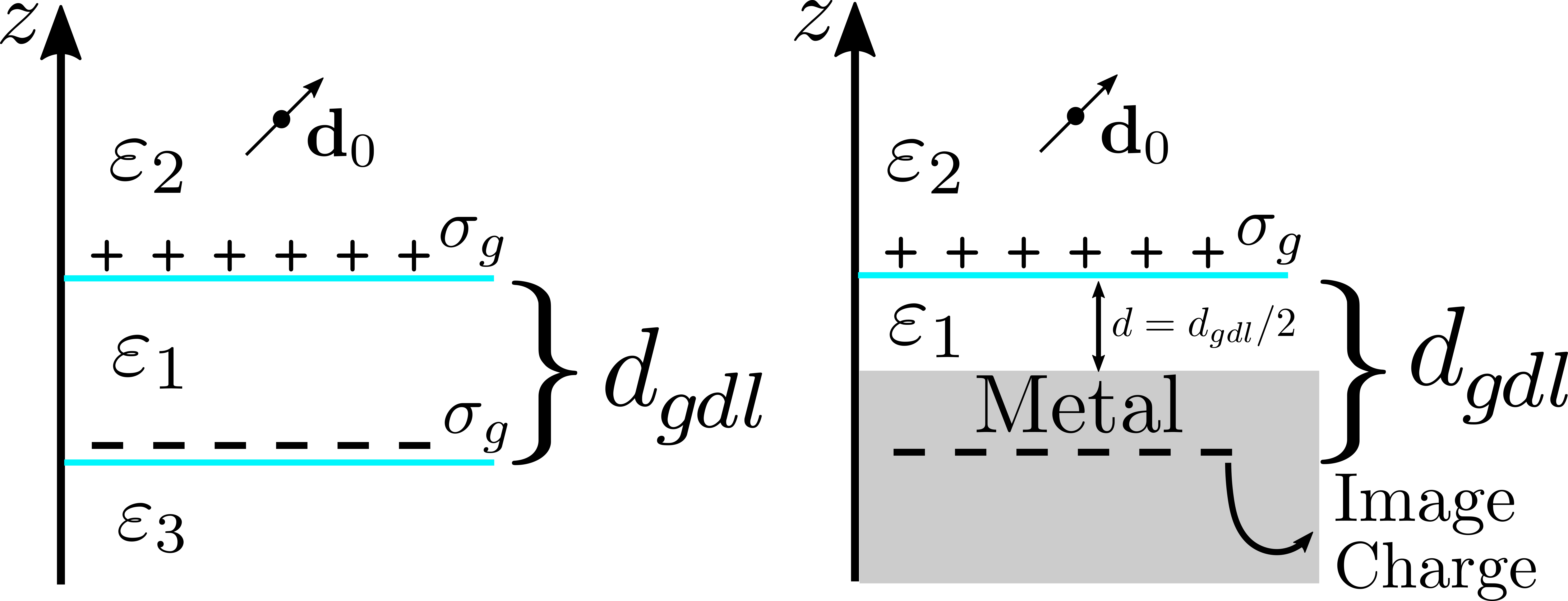
Figure 2: Comparison of the double layer graphene system and the graphene-metal case. Due to the image charges in the metal-graphene structure, the spectrum of the double layer graphene is equivalent to that of the graphene-metal system if we take into account that graphene is at at distance $d_{\text{gdl}}/2$ from the metal, where $d_{\text{gdl}}$ is the interlayer distance in the double layer case. Therefore, the graphene-metal distance has to be $d/2$ to obtain the same spectrum as for the graphene double layer . For a full numerical equivalence of the two spectra it is also necessary to have $\epsilon_{1}=\epsilon_{3}$ in the double layer geometry.

An alternative way to obtain the plasmon dispersion relation is to look for poles (or resonances in the presence of losses) in the so called loss function(Gonçalves and Peres, 2016) , which is defined as

$${\cal L}(\mathbf{q},\omega)=-\text{Im}\left[r_{p}(\mathbf{q},\omega)\right],$$ (71)

where $r_{p}(\mathbf{q},\omega)$ is the reflection coefficient of the structure in consideration for the $p$-polarization, and $\mathbf{q}$ and $\omega$ are the in-plane wavevector and frequency of the impingent radiation, respectively (see Appendix A). For a symmetric graphene double layer ($\epsilon_{1}=\epsilon_{3}$ and $\sigma_{g\text{top},L}=\sigma_{g\text{bot},L}$) and neglecting losses $\gamma\rightarrow 0$, this coefficient has poles at the solutions of Eqs. (70) and (69), as can be seen comparing those equations with Eq. (87). The loss function for the double layer graphene is depicted in the left panel of Fig. 3, as function of $\omega$ and of a dimensionless parameter $s=qc/\omega$ which defines the dispersion relation of the single graphene layer, clad by two different dielectrics of dielectric functions $\epsilon_{1}$ and $\epsilon_{2}$, in the electrostatic limit by

$$\omega(s)=\frac{4\alpha E_{F}}{\epsilon_{1}+\epsilon_{2}}s,$$ (72)

where $E_{F}$ is the Fermi energy of graphene and $\alpha$ is the fine structure constant of vacuum. In the top panel of Fig. 3 two branches are clearly seen: a high energy one – the optical branch – and the acoustic branch at lower energies. At high energies and high $s$ the two branches merge and converge to the single layer branch. The reader may wonder why the lower branch starts at finite momentum. This happens due to the definition of the $s$ parameter, which involves both the frequency and the real wavenumber $q$. This choice allows to clearly separate the two branches in the $(\omega,s)$ plane.

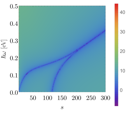
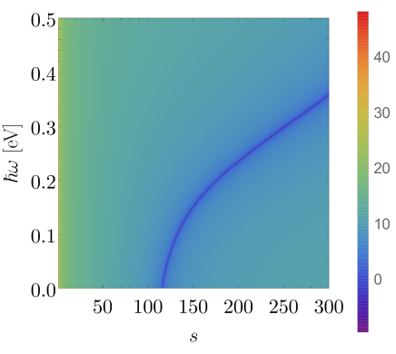
Figure 3: Loss function [Eq. (71)] for the $p$-polarization reflection coefficient for: (Top panel) a graphene double layer structure; (Bottom panel) graphene near a perfect metal. The parameters use in the top panel are $d_{\text{gdl}}=20$ nm, $\epsilon_{3}=1$, and for the bottom panel $d=10$ nm. The remaining parameters used in both panels are: $\epsilon_{1}=3.9$, $\epsilon_{2}=1$, $E_{F}=0.2$ eV and $\hbar\gamma=10$ meV. In both plots, non-local effects were neglected ($\beta=0$).

V Application: quantum emission close to graphene structures

We will now apply the quantization of the plasmon modes in grahene structures to the problem of spontaneous emission by a quantum emitter which is located above the structure. We model the quantum emitter as a two-level system embedded in medium $2$ at position $\mathbf{r}_{0}=\left(0,0,z_{0}\right)$. The quantum emitter couples to the plasmonic field via dipolar coupling:$\hat{H}_{\text{sp-d}}=-\hat{\mathbf{d}}\cdot\hat{\mathbf{E}}_{\text{\text{sp}}}(\mathbf{r}_{0}),$ with

$$\hat{\mathbf{d}} =\mathbf{d}_{ge}\hat{c}_{g}^{\dagger}\hat{c}_{e}+\text{h.c.}$$ (73)

$$\hat{\mathbf{E}}_{\text{sp}}(\mathbf{r}) =\sum_{\mathbf{q}}\left(i\sqrt{\frac{\hbar\omega_{\mathbf{q},\text{sp}}}{2S\epsilon_{0}L_{\mathbf{q},\text{sp}}}}\mathbf{A}_{\mathbf{q},\text{sp}}(z)e^{i\mathbf{q}\cdot\mathbf{x}}\hat{a}_{\mathbf{q},\text{sp}}+\text{h.c.}\right)$$ (74)

where $\hat{c}_{g/e}^{\dagger}$($\hat{c}_{g/e}$) is the creation (annihilation) operator for the ground/excited state of the two-level system and $\mathbf{d}_{ge}=\left\langle g\left|\hat{\mathbf{d}}\right|e\right\rangle$ is the dipole matrix element.

The transition rate of an emitter due to emission of surface plasmons in graphene is given by Fermi’s golden rule (Novotny and Hecht, 2006; Archambault et al., 2010):

$$\Gamma_{\text{sp}}=\frac{2\pi}{\hbar}\sum_{\mathbf{q}}\left|\left\langle g;n_{\mathbf{q},\text{sp}}+1\right|\hat{\mathbf{d}}\cdot\hat{\mathbf{E}}\left|e;n_{\mathbf{q},\text{sp}}\right\rangle\right|^{2}\delta\left(\hbar\omega_{0}-\hbar\omega_{\mathbf{q},\text{sp}}\right),$$ (75)

where $\omega_{0}$ is the transition frequency, $\left|g;n_{\mathbf{q},\text{sp}}+1\right\rangle$ represents a final state with one more surface plasmon and the emitter in the ground state and $\left|e;n_{\mathbf{q},\text{sp}}\right\rangle$ represents an initial state with $n_{\mathbf{q},\text{sp}}$ plasmons in graphene and the emitter in the excited state. The transition matrix element for spontaneous plasmon emission, when there are no surface plasmons in the initial state,is given by

$$\left\langle g;1\right|\hat{\mathbf{d}}\cdot\hat{\mathbf{E}}\left|e;0\right\rangle=i\sqrt{\frac{\hbar\omega_{\mathbf{q},\text{sp}}}{2S\epsilon_{0}L_{\mathbf{q},\text{sp}}}}\mathbf{d}_{ge}\cdot\mathbf{A}_{\mathbf{q},\text{sp}}^{*}(z_{0}),$$ (76)

With this result the transition rate reads

$$\Gamma_{\text{sp}}=\frac{1}{4\pi\hbar\epsilon_{0}}\int d^{2}\mathbf{q}\frac{\hbar\omega_{\mathbf{q},\text{sp}}}{L_{\mathbf{q},\text{sp}}}\left|\mathbf{d}_{ge}\cdot\mathbf{A}_{\mathbf{q},\text{sp}}^{*}(z_{0})\right|^{2}\times\\ \times\delta\left(\hbar\omega_{0}-\hbar\omega_{\mathbf{q},\text{sp}}\right),$$ (77)

Using the mode-function we can write

$$\left|\mathbf{d}_{ge}\cdot\mathbf{A}_{\mathbf{q},\text{sp}}^{*}(z_{0})\right|^{2}=\mathcal{N}_{\mathbf{q}}\left|\mathbf{d}_{ge}\right|^{2}e^{-2\kappa_{2,\mathbf{q}}z_{0}}\times\\ \times\left(\cos^{2}\phi\sin^{2}\psi+\frac{q^{2}}{\kappa_{2,\mathbf{q}}^{2}}\cos^{2}\psi\right),$$ (78)

$\psi$ is the angle the dipole makes with the axis perpendicular to graphene ($z$-axis), and $\phi$ is the azimuthal angle. The prefactor $\mathcal{N}_{\mathbf{q}}$ is define as $\mathcal{N}_{\mathbf{q}}=1$ for the single-layer graphene case and as $\mathcal{N}_{\mathbf{q}}=\sinh^{2}\left(\kappa_{1,\mathbf{q}}d\right)$ for the graphene+metal structure. Using the in-plane isotropy of the system, the momentum integration in Eq. (77) can be trivially performed, yielding:

$$\Gamma_{\text{sp}}=\mathcal{N}_{\mathbf{q}_{0}}\frac{q_{0}\omega_{\mathbf{q}_{0},\text{sp}}}{L_{\mathbf{q}_{0},\text{sp}}}\left(\frac{\partial\omega_{\mathbf{q}_{0},\text{sp}}}{\partial q}\right)^{-1}\frac{\left|\mathbf{d}_{ge}\right|^{2}}{4\hbar\epsilon_{0}}e^{-2\kappa_{2,\mathbf{q}_{0}}z_{0}}\times\\ \times\left(\sin^{2}\psi+2\frac{q^{2}}{\kappa_{2,\mathbf{q}_{0}}^{2}}\cos^{2}\psi\right),$$ (79)

where $q_{0}$ is the momentum of a surface plasmon, with frequency $\omega_{0}$, i.e., $\omega_{0}=\omega_{\mathbf{q}_{0},\text{sp}}$. So far the expression for $\Gamma_{\text{sp}}$ is general. The differences arise from the particular forms of the dispersion $\omega_{\mathbf{q},\text{sp}}$, the mode length $L_{\mathbf{q},\text{sp}}$ and the prefactor $\mathcal{N}_{\mathbf{q}}$.

V.1 Decay rate for local conductivity

We will now study the plasmon emission rate, when non-local effects are neglected, $\beta=0$ in Eq. (50).

We first focus on the case of a quantum emitter close to a single graphene layer and the same dielectric above and bellow the graphene layer, $\epsilon_{1}=\epsilon_{2}=\epsilon$. Using the analytic solution of Eq. (58) for this case, we can write Eq. (79) as

$$\Gamma_{\text{sp}}^{\text{gsl}}=\frac{d_{ge}^{2}}{4\hbar\epsilon_{0}}\left[2\omega_{0}^{4}\left(\frac{\hbar}{2\alpha E_{F}c}\right)^{2}+\frac{\omega_{0}^{2}\epsilon}{c^{2}}\right]\frac{e^{-2\kappa_{\mathbf{q}}z_{0}}}{L_{\mathbf{q}_{0},\text{sp}}}\times\\ \times\left[\sin^{2}\psi+2\kappa^{-2}\left[\omega_{0}^{4}\left(\frac{\hbar}{2\alpha E_{F}c}\right)^{2}+\frac{\omega_{0}^{2}\epsilon}{c^{2}}\right]\cos^{2}\psi\right].$$ (80)

In Figs. 4 and5, we plot the ratio $\Gamma_{\text{sp}}^{\text{gsl}}/\Gamma_{0}$, where $\Gamma_{0}=d_{ge}^{2}\omega_{0}^{3}/\left(3\pi\epsilon_{0}\hbar c^{3}\right)$ the total decay rate of an emitter in vacuum, for different graphene-quantum emitter distances $z_{0}$ and dipole orientations. For comparison, we will display the ratio $\Gamma_{\text{full}}/\Gamma_{0}$, where $\Gamma_{\text{full}}$ is the total decay rate (including both plasmon and photonic losses) of the quantum emitter. The total decay rate can be computed from the knowledge of the reflection coefficients, which are incorporated into the dyadic EM Green’s function (Agarwal, 1975b; Novotny and Hecht, 2006; Gonçalves and Peres, 2016) (see Ref. (Koppens et al., 2011) for a detailed study of the properties of an emitter near graphene using Dyadic Green’s functions). For a dipole in medium $n=2$, the total decay rate is given by

$$\frac{\Gamma_{\text{full}}}{\Gamma_{0}} =1+\frac{3}{2}\cos^{2}\psi\text{Re}\left(\int_{0}^{\infty}\frac{dq}{k_{1}^{3}}\frac{q^{3}}{k_{z,1}}r_{p}e^{-2\kappa_{2}z_{0}}\right)$$

$$+\frac{3}{4}\sin^{2}\psi\text{Re}\left(\int_{0}^{\infty}\frac{dq}{k_{1}}\frac{q}{k_{z,1}}\left(r_{s}-r_{p}\frac{c^{2}q^{2}}{\omega^{2}}\right)e^{-2\kappa_{2}z_{0}}\right),$$ (81)

where $r_{s/p}$ are reflection coefficients for the $s/p$-polarization and $k_{n}=\omega/c_{n}$ and $k_{z,n}$ are defined in Appendix A.

Figure 4: Decay rate of a quantum emitter close to a single graphene layer as a function of emitter frequency, for different emitter-graphene distances $z_{0}$. The solid lines show the decay rate due to plasmon emission as evaluated with Eq. (80). The dashed lines show the total decay rate computed used Eq. (81). The parameters used are $\epsilon_{1}=\epsilon_{2}=1$, $E_{F}=0.3$ eV, and $\cos^{2}\psi=1/3$. For the evaluation of the total decay rate a broadening of $\hbar\gamma=4$ meV was used. The local form of graphene conductivity was used $(\beta=0)$.

Figure 5: Decay rate of a quantum emitter close to a single graphene layer as a function of emitter frequency, for different dipole orientations: $\psi=0$ and $\psi=\pi/3$. Solid lines show the emission rate [Eq. (80)] and the dashed lines show the total decay rate [Eq. (81)]. The parameters considered where $z_{0}=70$ nm, $E_{F}=0.4$ eV, and $\epsilon_{1}=\epsilon_{2}=1$. In the evaluation of the total decay rate a broadening factor of $\hbar\gamma=0.1$ meV was used. For such small losses, the decay rate is completely dominated by the plasmon emission. The local form of graphene conductivity was used $(\beta=0)$.

A number of details are worth mentioning. There are two distinct behaviors of the decay rate $\Gamma_{\text{full}}$. At low frequency the curves shoot up due to Ohmic losses, which are not included in Eq. (80). At intermediate frequencies, the curves develop a clear resonance due to the excitation of surface plasmons in graphene. Also the maximum of the resonances blue-shifts with the decrease of the distance of the dipole to the graphene sheet. This behavior is easily explained remembering that the dispersion of the surface plasmons in single layer graphene is proportional to $\sqrt{q}$. Since the distance $z_{0}$ introduces a momentum scale $q\sim 1/z_{0}$, smaller $z_{0}$ values correspond to higher $q$-values and higher energies of the resonant maximum. Equation (80) for the plasmon emission rate produces exactly the same resonance (same magnitude and same maximum of the resonance position) as $\Gamma_{\text{full}}$, indicating that in this region, the decay rate of the quantum emitter is dominated by plasmon emission. This is further shown in Fig. 5, where losses were arbitrarily reduced in the evaluation of $\Gamma_{\text{full}}$. We can also avoid the superposition of the Ohmic and surface plasmon contributions choosing either a larger Fermi energy or a larger distance from graphene to the metal. In Fig. 5 the ratio $\Gamma/\Gamma_{0}$ is smaller than the ones in Fig. 4 due to the larger distance of the dipole to the graphene sheet.

An analytic expression for the plasmon emission rate can be also obtained for the case of graphene-metal structure assuming that $\kappa_{1}d\ll 1$. In this limit, Eq. 64 can be approximately solved, yielding $\hbar\omega_{\mathbf{q},\text{sp}}=\sqrt{4\alpha dE_{F}\hbar c/\epsilon}q$. Plugging this result in Eq. 79, we obtain

$$\Gamma_{\text{sp}}^{\text{gm}}\simeq\frac{d_{12}^{2}}{4\varepsilon_{0}\hbar}\frac{\varepsilon\sinh^{2}(\kappa_{1}d)}{4\alpha dE_{F}\hbar c}\frac{(\hbar\omega_{0})^{2}e^{-2\kappa_{2}z_{0}}}{L_{sq}(\omega_{at})}\\ \times\left(\sin^{2}\psi+2\frac{q^{2}}{\kappa_{2}^{2}}\cos^{2}\psi\right).$$ (82)

This plasmon emission rate is shown in Fig. 6 as a function of $\omega$ and the graphene-metal separation $d$. As in the case of a single graphene layer, for each $d$ there is a well defined peak as function of $\omega$.

Figure 6: Density plot of the transition rate of a quantum emitter due to the emission of surface plasmons in a graphene-metal structure. The used parameters are $z_{0}=30$ nm, $E_{F}=0.2$ eV, $\epsilon_{1}=3.9$, and $\epsilon_{2}=1$, $\psi=0$. Making line cuts at constant $d$ we can easily see the presence of a resonance in the dipole transition rate due to the excitation of graphene screened plasmons.

V.2 Decay rate with non-local effects

We now focus on the role of non-local effects in the graphene conductivity play in the emitter decay rate. We will restrict ourselves to the case of a quantum emitter close to a single layer of graphene. In Fig. 7, we compare the transition rate of a quantum emitter calculated taking into account non-local effects $\beta\neq 0$ in Eq. (37), with the local case $\beta=0$. The left panel shows the result for $E_{F}=0.6$ eV, $z_{0}=7$ nm, while the right panel shows the result for$E_{F}=0.6$ eV, $z_{0}=2$ nm. We can see that the nonlocal effects play an important role at smaller emitter-graphene distances. As the distance between quantum emitter and the graphene layer, $z_{0}$, decreases, non-locality leads to an increase and blueshift of the resonance in the transition rate as a function of the emitter frequency. We have also verified (not shown) that the non-local effects are also more prominent in the case of lower electronic densities.

Figure 7: Comparison between the plasmon emission rate of a quantum emitter close to a single layer of graphene using the local ($\beta=0$) and non-local (hydr.) ($\beta\neq 0$) models for the graphene conductivity (see Eq. (37)). The used $E_{F}=0.6$ eV, $\epsilon_{1}=\epsilon_{2}=3.9$, $\psi=0$. Left panel : $z_{0}=7$ nm. Right panel: $z_{0}=2$ nm. The nonlocal effects causes an increase and blueshift of the resonance in the transition rate as the distance $z_{0}$ between the quantum emitter and the graphene decreases.

VI Conclusions

In this paper, we have performed the quantization of graphene plasmons, in the absence of losses, and applied the field quantization to the interaction of an emitter with doped graphene. The quantization was performed using both a macroscopic energy approach and a quantum hydrodynamic model, which allows for the inclusion of non-local effects in the EM response of graphene. The quantization approaches used allow for the determination of the plasmon EM field mode-functions and, importantly, their normalization, which becomes non-trivial when dispersion is included.

When comparing the total decay rate of a quantum emitter (as obtained using the full EM dyadic Green’s function) with the decay rate due to quantum emission, it was shown that plasmon emission completely dominates the decay rate, for typical emitter-graphene separations and emitter frequencies. It was shown that non-local effects in the graphene response, become increasingly important for smaller graphene-emitter separations and smaller Fermi energies.

The advantage of the quantization method developed in this work lies in its simplicity. The mode-functions are obtained from the solution of the Maxwell equations for the vector potential, and the normalization of the mode-functions can be expressed as a simply integral, which only involves the dielectric function of the medium. For situations when only a few modes contribute significantly to the physics, as in the case of quantum emission dominated by plamons, mode-functions allows to a much simpler and physically transparent description than the full EM dyadic Green’s function. Since, the determination of the mode-functions only involves the solution of the classical Maxwell equations, the quantization of the electromagnetic field of more complexes structures can be easily achieved. We also note that the procedure gives both the quantized form of the electric and magnetic fields. Therefore, we could also study the enhancement of the spin relaxation. The only change would be the interaction Hamiltonian, which in this case would be of the form $H_{I}=-\bm{\mu}\cdot\mathbf{B}$, where $\bm{\mu}$ is the magnetic dipole moment of the emitter and $\mathbf{B}$ the quantized magnetic field of the surface plasmon.

In possession of a quantized theory for graphene plasmons, we have set the stage for the future discussion of other quantum effects involving these collective excitation made simultaneously of light and matter.

Appendix A Reflection coefficients of graphene structures

In this appendix we provide the reflection coefficients needed for the evaluation of the full decay rate of a quantum emitter, Eq. (81).

A.1 Reflection coefficients for a single graphene layer

The Fresnel problem for a single graphene sheet has been considered in Ref. (Gonçalves and Peres, 2016). Therefore we provide here the final results only and for simplicity we assume we are dealing with non-magnetic media. For an incoming wave from region $2$, and for the $s-$polarization the reflection and transmission coefficient read

$$r_{s} = \frac{k_{z,2}-k_{z,1}-\mu_{0}\omega\sigma_{g,T}}{k_{z,2}+k_{z,1}+\mu_{0}\omega\sigma_{g}},$$ (83)

$$t_{s} = \frac{2k_{z,2}}{k_{z,2}+k_{z,1}+\mu_{0}\omega\sigma_{g,T}},$$ (84)

whereas for the $p-$polarization we have

$$r_{p} = -\frac{\epsilon_{2}k_{z,1}-\epsilon_{1}k_{z,2}-k_{z,1}k_{z,2}\sigma_{g,L}/\left(\omega\epsilon_{0}\right)}{\epsilon_{2}k_{z,1}+\epsilon_{1}k_{z,2}+k_{z,1}k_{z,2}\sigma_{g,L}/\left(\omega\epsilon_{0}\right)},$$ (85)

$$t_{p} = \sqrt{\frac{\epsilon_{1}}{\epsilon_{2}}}\frac{2k_{z,2}\epsilon_{1}}{\epsilon_{2}k_{z,1}+\epsilon_{1}k_{z,2}+k_{z,1}k_{z,2}\sigma_{g,L}/\left(\omega\epsilon_{0}\right)}.$$ (86)

In these equations, we have $k_{z,n}=\sqrt{\epsilon_{n}\omega^{2}/c^{2}-q^{2}}=i\kappa_{n}$, and $\sigma_{g,L/T}$ is the optical longitudinal/transverse conductivity of graphene, $\epsilon_{0}$ and $\mu_{0}$ are the vacuum permitivity and permeability, respectively, $q$ is the wavenumber along the graphene sheet, and $\omega$ is the frequency of the electromagnetic radiation.

A.2 Metal-graphene reflectance coefficient

The reflection coefficient for the $p$-polarization for this structure is given by

$$r_{p}=1-\frac{2k_{z,1}k_{2}^{2}\sin\left(k_{z,1}d\right)}{k_{z,1}\sin\left(k_{z,1}d\right)\left(k_{z,2}\mu_{0}\omega\sigma_{g,L}+k_{2}^{2}\right)+ik_{z,2}k_{1}^{2}\cos\left(k_{z,1}d\right)},$$ (87)

where $k_{n}^{2}=\epsilon_{n}\omega^{2}/c^{2}$, $d$ is the graphene-metal distance, and $\kappa_{n}^{2}=k_{n}^{2}-q^{2}$, where $q$ is the wavenumber along the graphene sheet. For the $s-$polarization we have

$$r_{s}=-1+\frac{2k_{z,2}\sin\left(k_{z,1}d\right)}{\sin\left(k_{z,1}d\right)\left(k_{z,2}+\mu_{0}\omega\sigma_{g,T}\right)+ik_{z,1}\cos\left(k_{z,1}d\right)}.$$ (88)

Appendix B Diagonalization of Hydrodynamic Hamiltonian

B.1 Orthogonality of mode-functions

We start by showing that the mode-functions $\left(\mathbf{A}_{\mathbf{q},\lambda}(z),\,\bm{\upsilon}_{\mathbf{q},\lambda}\right)$ obey certain orthogonality conditions which will be useful. We start by writing the equations for the mode-functions within the hydrodynamic model, Eqs. (32) and (33), in matrix form as

$$\left[\begin{array}[]{cc}\omega_{\mathbf{q},\lambda}^{2}\epsilon_{0}\bar{\epsilon}_{d}(z)-\frac{1}{\mu_{0}}D_{\mathbf{q}}\times D_{\mathbf{q}}\times&i\omega_{\mathbf{q},\lambda}en_{0}\delta(z)\\ -i\omega_{\mathbf{q},\lambda}en_{0}\delta(z)&n_{0}m\left(\omega_{\mathbf{q},\lambda}^{2}-\beta^{2}\mathbf{q}\otimes\mathbf{q}\right)\delta(z)\end{array}\right]\left[\begin{array}[]{c}\mathbf{A}_{\mathbf{q},\lambda}(z)\\ \bm{\upsilon}_{\mathbf{q},\lambda}\end{array}\right]=0.$$ (89)

Let us now consider another mode $\lambda^{\prime}$, with mode-function $\left(\mathbf{A}_{\mathbf{q},\lambda^{\prime}}(z),\,\bm{\upsilon}_{\mathbf{q},\lambda^{\prime}}\right)$, solution of

$$\left[\begin{array}[]{cc}\omega_{\mathbf{q},\lambda^{\prime}}^{2}\epsilon_{0}\bar{\epsilon}_{d}(z)-\frac{1}{\mu_{0}}D_{\mathbf{q}}\times D_{\mathbf{q}}\times&i\omega_{\mathbf{q},\lambda^{\prime}}en_{0}\delta(z)\\ -i\omega_{\mathbf{q},\lambda^{\prime}}en_{0}\delta(z)&n_{0}m\left(\omega_{\mathbf{q},\lambda^{\prime}}^{2}-\beta^{2}\mathbf{q}\otimes\mathbf{q}\right)\delta(z)\end{array}\right]\left[\begin{array}[]{c}\mathbf{A}_{\mathbf{q},\lambda^{\prime}}(z)\\ \bm{\upsilon}_{\mathbf{q},\lambda^{\prime}}\end{array}\right]=0.$$ (90)

Now we contract Eq. (89) with $\left[\begin{array}[]{cc}\mathbf{A}_{\mathbf{q},\lambda^{\prime}}^{\dagger}(z)&\bm{\upsilon}_{\mathbf{q},\lambda^{\prime}}^{\dagger}\end{array}\right]$, Eq. (89) with $\left[\begin{array}[]{cc}\mathbf{A}_{\mathbf{q},\lambda}^{\dagger}(z)&\bm{\upsilon}_{\mathbf{q},\lambda}^{\dagger}\end{array}\right]$ and integrate both equations over $z$ obtaining

$$\int dz\left[\begin{array}[]{cc}\mathbf{A}_{\mathbf{q},\lambda^{\prime}}^{\dagger}(z)&\bm{\upsilon}_{\mathbf{q},\lambda^{\prime}}^{\dagger}\end{array}\right]\left[\begin{array}[]{cc}\omega_{\mathbf{q},\lambda}^{2}\epsilon_{0}\bar{\epsilon}_{d}(z)-\frac{1}{\mu_{0}}D_{\mathbf{q}}\times D_{\mathbf{q}}\times&i\omega_{\mathbf{q},\lambda}en_{0}\delta(z)\\ -i\omega_{\mathbf{q},\lambda}en_{0}\delta(z)&n_{0}m\left(\omega_{\mathbf{q},\lambda}^{2}-\beta^{2}\mathbf{q}\otimes\mathbf{q}\right)\delta(z)\end{array}\right]\left[\begin{array}[]{c}\mathbf{A}_{\mathbf{q},\lambda}(z)\\ \bm{\upsilon}_{\mathbf{q},\lambda}\end{array}\right] =0,$$ (96)

$$\int dz\left[\begin{array}[]{cc}\mathbf{A}_{\mathbf{q},\lambda}^{\dagger}(z)&\bm{\upsilon}_{\mathbf{q},\lambda}^{\dagger}\end{array}\right]\left[\begin{array}[]{cc}\omega_{\mathbf{q},\lambda^{\prime}}^{2}\epsilon_{0}\bar{\epsilon}_{d}(z)-\frac{1}{\mu_{0}}D_{\mathbf{q}}\times D_{\mathbf{q}}\times&i\omega_{\mathbf{q},\lambda^{\prime}}en_{0}\delta(z)\\ -i\omega_{\mathbf{q},\lambda^{\prime}}en_{0}\delta(z)&n_{0}m\left(\omega_{\mathbf{q},\lambda^{\prime}}^{2}-\beta^{2}\mathbf{q}\otimes\mathbf{q}\right)\delta(z)\end{array}\right]\left[\begin{array}[]{c}\mathbf{A}_{\mathbf{q},\lambda^{\prime}}(z)\\ \bm{\upsilon}_{\mathbf{q},\lambda^{\prime}}\end{array}\right] =0.$$ (102)

Taking the conjugate of Eq. (102), we obtain

$$\int dz\left[\begin{array}[]{cc}\mathbf{A}_{\mathbf{q},\lambda^{\prime}}^{\dagger}(z)&\bm{\upsilon}_{\mathbf{q},\lambda^{\prime}}^{\dagger}\end{array}\right]\left[\begin{array}[]{cc}\omega_{\mathbf{q},\lambda^{\prime}}^{2}\epsilon_{0}\bar{\epsilon}_{d}(z)-\frac{1}{\mu_{0}}D_{\mathbf{q}}\times D_{\mathbf{q}}\times&i\omega_{\mathbf{q},\lambda^{\prime}}en_{0}\delta(z)\\ -i\omega_{\mathbf{q},\lambda^{\prime}}en_{0}\delta(z)&n_{0}m\left(\omega_{\mathbf{q},\lambda^{\prime}}^{2}-\beta^{2}\mathbf{q}\otimes\mathbf{q}\right)\delta(z)\end{array}\right]\left[\begin{array}[]{c}\mathbf{A}_{\mathbf{q},\lambda}(z)\\ \bm{\upsilon}_{\mathbf{q},\lambda}\end{array}\right]=0.$$ (103)

Subtracting this last equation from Eq. (96), we obtain

$$\int dz\left[\begin{array}[]{cc}\mathbf{A}_{\mathbf{q},\lambda^{\prime}}^{\dagger}(z)&\bm{\upsilon}_{\mathbf{q},\lambda^{\prime}}^{\dagger}\end{array}\right]\left[\begin{array}[]{cc}\left(\omega_{\mathbf{q},\lambda}^{2}-\omega_{\mathbf{q},\lambda^{\prime}}^{2}\right)\epsilon_{0}\bar{\epsilon}_{d}(z)&i\left(\omega_{\mathbf{q},\lambda}-\omega_{\mathbf{q},\lambda^{\prime}}\right)en_{0}\delta(z)\\ -i\left(\omega_{\mathbf{q},\lambda}-\omega_{\mathbf{q},\lambda^{\prime}}\right)en_{0}\delta(z)&n_{0}m\left(\omega_{\mathbf{q},\lambda}^{2}-\omega_{\mathbf{q},\lambda^{\prime}}^{2}\right)\delta(z)\end{array}\right]\left[\begin{array}[]{c}\mathbf{A}_{\mathbf{q},\lambda}(z)\\ \bm{\upsilon}_{\mathbf{q},\lambda}\end{array}\right]=0.$$ (104)

If $\omega_{\mathbf{q},\lambda}\neq\omega_{\mathbf{q},\lambda^{\prime}}$, we can divide by $\omega_{\mathbf{q},\lambda}-\omega_{\mathbf{q},\lambda^{\prime}}$ obtaining one of the orthogonality conditions:

$$\int dz\left[\begin{array}[]{cc}\mathbf{A}_{\mathbf{q},\lambda^{\prime}}^{\dagger}(z)&\bm{\upsilon}_{\mathbf{q},\lambda^{\prime}}^{\dagger}\end{array}\right]\left[\begin{array}[]{cc}\left(\omega_{\mathbf{q},\lambda}+\omega_{\mathbf{q},\lambda^{\prime}}\right)\epsilon_{0}\bar{\epsilon}_{d}(z)&ien_{0}\delta(z)\\ -ien_{0}\delta(z)&n_{0}m\left(\omega_{\mathbf{q},\lambda}-\omega_{\mathbf{q},\lambda^{\prime}}\right)\delta(z)\end{array}\right]\left[\begin{array}[]{c}\mathbf{A}_{\mathbf{q},\lambda}(z)\\ \bm{\upsilon}_{\mathbf{q},\lambda}\end{array}\right]=0.$$ (105)

We can obtain an additional orthogonality relation. If we take the complex conjugate of Eq. (96), replace $\mathbf{q}\rightarrow-\mathbf{q}$ and $\lambda\rightarrow\lambda^{\prime}$, and using the fact that $\omega_{\mathbf{q},\lambda}=\omega_{-\mathbf{q},\lambda}$, we obtain

$$\left[\begin{array}[]{cc}\omega_{\mathbf{q},\lambda^{\prime}}^{2}\epsilon_{0}\bar{\epsilon}_{d}(z)-\frac{1}{\mu_{0}}D_{\mathbf{q}}\times D_{\mathbf{q}}\times&-i\omega_{\mathbf{q},\lambda^{\prime}}en_{0}\delta(z)\\ i\omega_{\mathbf{q},\lambda^{\prime}}en_{0}\delta(z)&n_{0}m\left(\omega_{\mathbf{q},\lambda^{\prime}}^{2}-\beta^{2}\mathbf{q}\otimes\mathbf{q}\right)\delta(z)\end{array}\right]\left[\begin{array}[]{c}\mathbf{A}_{-\mathbf{q},\lambda}^{*}(z)\\ \bm{\upsilon}_{-\mathbf{q},\lambda}^{*}\end{array}\right]=0.$$ (106)

We now contract this equation with $\left[\begin{array}[]{cc}\mathbf{A}_{\mathbf{q},\lambda}^{\dagger}(z)&\bm{\upsilon}_{\mathbf{q},\lambda}^{\dagger}\end{array}\right]$, integrate over $z$ and take its complex conjugate, obtaining

$$\int dz\left[\begin{array}[]{cc}\mathbf{A}_{-\mathbf{q},\lambda}^{t}(z)&\bm{\upsilon}_{-\mathbf{q},\lambda}^{t}\end{array}\right]\left[\begin{array}[]{cc}\omega_{\mathbf{q},\lambda^{\prime}}^{2}\epsilon_{0}\bar{\epsilon}_{d}(z)-\frac{1}{\mu_{0}}D_{\mathbf{q}}\times D_{\mathbf{q}}\times&-i\omega_{\mathbf{q},\lambda^{\prime}}en_{0}\delta(z)\\ i\omega_{\mathbf{q},\lambda^{\prime}}en_{0}\delta(z)&n_{0}m\left(\omega_{\mathbf{q},\lambda^{\prime}}^{2}-\beta^{2}\mathbf{q}\otimes\mathbf{q}\right)\delta(z)\end{array}\right]\left[\begin{array}[]{c}\mathbf{A}_{\mathbf{q},\lambda}(z)\\ \bm{\upsilon}_{\mathbf{q},\lambda}\end{array}\right]=0.$$ (107)

Contracting Eq. (89) with $\left[\begin{array}[]{cc}\mathbf{A}_{-\mathbf{q},\lambda}^{t}(z)&\bm{\upsilon}_{-\mathbf{q},\lambda}^{t}\end{array}\right]$ and integrating over $z$ we obtain

$$\int dz\left[\begin{array}[]{cc}\mathbf{A}_{-\mathbf{q},\lambda}^{t}(z)&\bm{\upsilon}_{-\mathbf{q},\lambda}^{t}\end{array}\right]\left[\begin{array}[]{cc}\omega_{\mathbf{q},\lambda}^{2}\epsilon_{0}\bar{\epsilon}_{d}(z)-\frac{1}{\mu_{0}}D_{\mathbf{q}}\times D_{\mathbf{q}}\times&i\omega_{\mathbf{q},\lambda}en_{0}\delta(z)\\ -i\omega_{\mathbf{q},\lambda}en_{0}\delta(z)&n_{0}m\left(\omega_{\mathbf{q},\lambda}^{2}-\beta^{2}\mathbf{q}\otimes\mathbf{q}\right)\delta(z)\end{array}\right]\left[\begin{array}[]{c}\mathbf{A}_{\mathbf{q},\lambda}(z)\\ \bm{\upsilon}_{\mathbf{q},\lambda}\end{array}\right]=0.$$ (108)

Subtracting Eq. (107) from (108), we obtain

$$\int dz\left[\begin{array}[]{cc}\mathbf{A}_{-\mathbf{q},\lambda}^{t}(z)&\bm{\upsilon}_{-\mathbf{q},\lambda}^{t}\end{array}\right]\left[\begin{array}[]{cc}\left(\omega_{\mathbf{q},\lambda}^{2}-\omega_{\mathbf{q},\lambda^{\prime}}^{2}\right)\epsilon_{0}\bar{\epsilon}_{d}(z)&i\left(\omega_{\mathbf{q},\lambda}+\omega_{\mathbf{q},\lambda^{\prime}}\right)en_{0}\delta(z)\\ -i\left(\omega_{\mathbf{q},\lambda}+\omega_{\mathbf{q},\lambda^{\prime}}\right)en_{0}\delta(z)&n_{0}m\left(\omega_{\mathbf{q},\lambda}^{2}-\omega_{\mathbf{q},\lambda^{\prime}}^{2}\right)\delta(z)\end{array}\right]\left[\begin{array}[]{c}\mathbf{A}_{\mathbf{q},\lambda}(z)\\ \bm{\upsilon}_{\mathbf{q},\lambda}\end{array}\right]=0.$$ (109)

For $\omega_{\mathbf{q},\lambda}+\omega_{\mathbf{q},\lambda^{\prime}}\neq 0$, we obtain a second orthogonality condition:

$$\int dz\left[\begin{array}[]{cc}\mathbf{A}_{-\mathbf{q},\lambda}^{t}(z)&\bm{\upsilon}_{-\mathbf{q},\lambda}^{t}\end{array}\right]\left[\begin{array}[]{cc}\left(\omega_{\mathbf{q},\lambda}-\omega_{\mathbf{q},\lambda^{\prime}}\right)\epsilon_{0}\bar{\epsilon}_{d}(z)&ien_{0}\delta(z)\\ -ien_{0}\delta(z)&n_{0}m\left(\omega_{\mathbf{q},\lambda}-\omega_{\mathbf{q},\lambda^{\prime}}\right)\delta(z)\end{array}\right]\left[\begin{array}[]{c}\mathbf{A}_{\mathbf{q},\lambda}(z)\\ \bm{\upsilon}_{\mathbf{q},\lambda}\end{array}\right]=0.$$ (110)

B.2 Hamiltonian in term of mode amplitudes

We now insert the expansion of the fields in terms of mode-functions, Eqs. (30) and (31), into the classical Hamiltonian (29). Using Eqs. (27) and (28), we can write

$$H=\frac{1}{2}\sum_{\mathbf{q},\lambda\lambda^{\prime}}\left(h_{\mathbf{\lambda,\lambda^{\prime}}}(\mathbf{q})\alpha_{\mathbf{q},\lambda^{\prime}}^{*}(t)\alpha_{\mathbf{q},\lambda}(t)+\tilde{h}_{\mathbf{\lambda,\lambda^{\prime}}}(\mathbf{q})\alpha_{-\mathbf{q},\lambda^{\prime}}(t)\alpha_{\mathbf{q},\lambda}(t)\right)+\text{c.c.},$$ (111)

where

$$h_{\mathbf{\lambda,\lambda^{\prime}}}(\mathbf{q}) =\int dz\left[\begin{array}[]{cc}\mathbf{A}_{\mathbf{q},\lambda^{\prime}}^{\dagger}(z)&\bm{\upsilon}_{\mathbf{q},\lambda^{\prime}}^{\dagger}\end{array}\right]$$ (113)

$$\left[\begin{array}[]{cc}\omega_{\mathbf{q},\lambda^{\prime}}\omega_{\mathbf{q},\lambda}\epsilon_{0}\bar{\epsilon}_{d}(z)+\mu_{0}^{-1}D_{\mathbf{q}}\times D_{\mathbf{q}}&0\\ 0&\delta(z)\left(n_{0}m\omega_{\mathbf{q},\lambda^{\prime}}\omega_{\mathbf{q},\lambda}+n_{0}m\beta^{2}\mathbf{q}\otimes\mathbf{q}\right)\end{array}\right]\left[\begin{array}[]{c}\mathbf{A}_{\mathbf{q},\lambda}(z)\\ \bm{\upsilon}_{\mathbf{q},\lambda}\end{array}\right]$$ (118)

$$\tilde{h}_{\mathbf{\lambda,\lambda^{\prime}}}(\mathbf{q}) =\int dz\left[\begin{array}[]{cc}\mathbf{A}_{-\mathbf{q},\lambda^{\prime}}^{t}(z)&\bm{\upsilon}_{-\mathbf{q},\lambda^{\prime}}^{t}\end{array}\right]$$ (120)

$$\left[\begin{array}[]{cc}-\omega_{\mathbf{q},\lambda^{\prime}}\omega_{\mathbf{q},\lambda}\epsilon_{0}\bar{\epsilon}_{d}(z)+\mu_{0}^{-1}D_{\mathbf{q}}\times D_{\mathbf{q}}&0\\ 0&\delta(z)\left(-n_{0}m\omega_{\mathbf{q},\lambda^{\prime}}\omega_{\mathbf{q},\lambda}+n_{0}m\beta^{2}\mathbf{q}\otimes\mathbf{q}\right)\end{array}\right]\left[\begin{array}[]{c}\mathbf{A}_{\mathbf{q},\lambda}(z)\\ \bm{\upsilon}_{\mathbf{q},\lambda}\end{array}\right]$$ (125)

Using the mode-function equation (89), we can write

$$h_{\mathbf{\lambda,\lambda^{\prime}}}(\mathbf{q}) =\omega_{\mathbf{q},\lambda}\int dz\left[\begin{array}[]{cc}\mathbf{A}_{\mathbf{q},\lambda^{\prime}}^{\dagger}(z)&\bm{\upsilon}_{\mathbf{q},\lambda^{\prime}}^{\dagger}\end{array}\right]\left[\begin{array}[]{cc}\left(\omega_{\mathbf{q},\lambda^{\prime}}+\omega_{\mathbf{q},\lambda}\right)\epsilon_{0}\bar{\epsilon}_{d}(z)&ien_{0}\delta(z)\\ -ien_{0}\delta(z)&\delta(z)n_{0}m\left(\omega_{\mathbf{q},\lambda^{\prime}}+\omega_{\mathbf{q},\lambda}\right)\end{array}\right]\left[\begin{array}[]{c}\mathbf{A}_{\mathbf{q},\lambda}(z)\\ \bm{\upsilon}_{\mathbf{q},\lambda}\end{array}\right],$$ (131)

$$\tilde{h}_{\mathbf{\lambda,\lambda^{\prime}}}(\mathbf{q}) =\omega_{\mathbf{q},\lambda}\int dz\left[\begin{array}[]{cc}\mathbf{A}_{-\mathbf{q},\lambda^{\prime}}^{t}(z)&\bm{\upsilon}_{-\mathbf{q},\lambda^{\prime}}^{t}\end{array}\right]\left[\begin{array}[]{cc}\left(\omega_{\mathbf{q},\lambda}-\omega_{\mathbf{q},\lambda^{\prime}}\right)\epsilon_{0}\bar{\epsilon}_{d}(z)&ien_{0}\delta(z)\\ -ien_{0}\delta(z)&\delta(z)n_{0}m\left(\omega_{\mathbf{q},\lambda}-\omega_{\mathbf{q},\lambda^{\prime}}\right)\end{array}\right]\left[\begin{array}[]{c}\mathbf{A}_{\mathbf{q},\lambda}(z)\\ \bm{\upsilon}_{\mathbf{q},\lambda}\end{array}\right].$$ (137)

Using the orthogonality condition (110) we conclude that $\tilde{h}_{\mathbf{\lambda,\lambda^{\prime}}}(\mathbf{q})=0$. The orthogonality condition (105) implies that $h_{\mathbf{\lambda,\lambda^{\prime}}}(\mathbf{q})=0$, except when $\lambda=\lambda^{\prime}$ (assuming there are no degeneracies in $\omega_{\mathbf{q},\lambda}$). Therefore, we see that the classical Hamiltonian can be written as in Eq. (40), with the mode-length being biven by

$$L_{\mathbf{q},\lambda}=\frac{1}{2\epsilon_{0}\omega_{\mathbf{q},\lambda}^{2}}\int dz\left[\begin{array}[]{cc}\mathbf{A}_{\mathbf{q},\lambda^{\prime}}^{\dagger}(z)&\bm{\upsilon}_{\mathbf{q},\lambda^{\prime}}^{\dagger}\end{array}\right]\left[\begin{array}[]{cc}2\omega_{\mathbf{q},\lambda}^{2}\epsilon_{0}\bar{\epsilon}_{d}(z)&i\omega_{\mathbf{q},\lambda}en_{0}\delta(z)\\ -i\omega_{\mathbf{q},\lambda}en_{0}\delta(z)&2\omega_{\mathbf{q},\lambda}^{2}\delta(z)n_{0}m\end{array}\right]\left[\begin{array}[]{c}\mathbf{A}_{\mathbf{q},\lambda}(z)\\ \bm{\upsilon}_{\mathbf{q},\lambda}\end{array}\right],$$ (138)

which can be written as Eq. (41).

References

• Agarwal (2013) G. S. Agarwal, Quantum Optics, 1st ed. (Cambridge University Press, 2013).
• Heeres et al. (2013) R. W. Heeres, L. P. Kouwenhoven,  and V. Zwiller, Nat. Nano. 8, 719 (2013).
• Jacob (2012) Z. Jacob, MRS Bulletin 37, 761 (2012).
• Tame et al. (2013) M. S. Tame, K. R. McEnery, S. K. Ozdemir, J. Lee, S. A. Maier,  and M. S. Kim, Nat. Phys. 9, 329 (2013).
• Martín-Cano et al. (2014) D. Martín-Cano, P. A. Huidobro, E. Moreno,  and F. J. García-Vidal, in Modern Plasmonics, Vol. 4, edited by A. A. Maradudin, J. R. Sambles,  and W. L. Barnes (Elsevier, New York, 2014) 1st ed., Chap. 12, p. 349.
• Fakonas et al. (2015) J. S. Fakonas, A. Mitskovets,  and H. A. Atwater, New J. Phys. 17, 023002 (2015).
• Fitzgerald et al. (2016) J. M. Fitzgerald, P. Narang, R. V. Craster, S. A. Maier,  and V. Giannini, Proceedings of the IEEE 104, 2307 (2016).
• Dheur et al. (2016) M.-C. Dheur, E. Devaux, T. W. Ebbesen, A. Baron, J.-C. Rodier, J.-P. Hugonin, P. Lalanne, J.-J. Greffet, G. Messin,  and F. Marquier, Science Advances 2, e1501574 (2016).
• Bozhevolnyi and Mortensen (2017) S. Bozhevolnyi and N. Mortensen, Nanophotonics 6, 1185 (2017).
• Xu et al. (2018) D. Xu, X. Xiong, L. Wu, X.-F. Ren, C. E. Png, G.-C. Guo, Q. Gong,  and Y.-F. Xiao, Advances in Optics and Photonics 10, 703 (2018).
• Fernández-Domínguez et al. (2018) A. I. Fernández-Domínguez, S. I. Bozhevolnyi,  and N. A. Mortensen, ACS Photonics 5, 3447 (2018).
• Ju et al. (2011) L. Ju, B. Geng, J. Horng, C. Girit, M. Martin, Z. Hao, H. A. Bechtel, X. Liang, A. Zettl, Y. R. Shen,  and F. Wang, Nat. Nano. 6, 630 (2011).
• Fei et al. (2011) Z. Fei, G. O. Andreev, W. Bao, L. M. Zhang, A. S. Mcleod, C. Wang, M. K. Stewart, Z. Zhao, G. Dominguez, M. Thiemens, M. M. Fogler, M. J. Tauber, A. H. Castro-neto, C. N. Lau, F. Keilmann,  and D. N. Basov, Nano Lett. 11, 4701 (2011).
• Fei et al. (2012) Z. Fei, A. S. Rodin, G. O. Andreev, W. Bao, A. S. McLeod, M. Wagner, L. M. Zhang, Z. Zhao, M. Thiemens, G. Dominguez, M. M. Fogler, A. H. C. Neto, C. N. Lau, F. Keilmann,  and D. N. Basov, Nature 487, 82 (2012).
• Chen et al. (2012) J. Chen, M. Badioli, P. Alonso-González, S. Thongrattanasiri, F. Huth, J. Osmond, M. Spasenović, A. Centeno, A. Pesquera, P. Godignon, A. Zurutuza Elorza, N. Camara, F. J. G. de Abajo, R. Hillenbrand,  and F. H. L. Koppens, Nature 487, 77 (2012).
• Woessner et al. (2015) A. Woessner, M. B. Lundeberg, Y. Gao, A. Principi, M. Carrega, K. Watanabe, T. Taniguchi, G. Vignale, M. Polini, J. Hone, R. Hillenbrand,  and F. H. L. Koppens, Nat. Mat. 14, 421 (2015).
• Alcaraz Iranzo et al. (2018) D. Alcaraz Iranzo, S. Nanot, E. J. C. Dias, I. Epstein, C. Peng, D. K. Efetov, M. B. Lundeberg, R. Parret, J. Osmond, J.-Y. Hong, J. Kong, D. R. Englund, N. M. R. Peres,  and F. H. L. Koppens, Science 360, 291 (2018).
• Lundeberg et al. (2017) M. B. Lundeberg, Y. Gao, R. Asgari, C. Tan, B. Van Duppen, M. Autore, P. Alonso-González, A. Woessner, K. Watanabe, T. Taniguchi, R. Hillenbrand, J. Hone, M. Polini,  and F. H. L. Koppens, Science 357, 187 (2017).
• Dias et al. (2018) E. J. C. Dias, D. A. Iranzo, P. A. D. Gonçalves, Y. Hajati, Y. V. Bludov, A.-P. Jauho, N. A. Mortensen, F. H. L. Koppens,  and N. M. R. Peres, Phys. Rev. B 97, 245405 (2018).
• Chang et al. (2006) D. E. Chang, A. S. Sørensen, P. R. Hemmer,  and M. D. Lukin, Phys. Rev. Lett. 97, 053002 (2006).
• Alpeggiani and Andreani (2014) F. Alpeggiani and L. C. Andreani, Plasmonics 9, 965 (2014).
• Bordo (2019) V. G. Bordo, Journal of the Optical Society of America B 36, 323 (2019).
• Hopfield (1958) J. J. Hopfield, Phys. Rev. 112, 1555 (1958).
• Alekseev and Nikitin (1966) A. Alekseev and Y. P. Nikitin, Sov. Phys. JETP 23, 608 (1966).
• Agarwal (1975a) G. S. Agarwal, Phys. Rev. A 11, 230 (1975a).
• Huttner and Barnett (1992) B. Huttner and S. M. Barnett, Phys. Rev. A 46, 4306 (1992).
• Milonni (1995) P. Milonni, J. Mod. Opt. 42, 1991 (1995).
• Gruner and Welsch (1995) T. Gruner and D.-G. Welsch, Phys. Rev. A 51, 3246 (1995).
• Gruner and Welsch (1996) T. Gruner and D.-G. Welsch, Phys. Rev. A 53, 1818 (1996).
• Matloob et al. (1995) R. Matloob, R. Loudon, S. M. Barnett,  and J. Jeffers, Phys. Rev. A 52, 4823 (1995).
• Dung et al. (1998) H. T. Dung, L. Knöll,  and D.-G. Welsch, Phys. Rev. A 57, 3931 (1998).
• Philbin (2010) T. G. Philbin, New Journal of Physics 12, 123008 (2010).
• Hanson et al. (2015) G. W. Hanson, S. A. Hassani Gangaraj, C. Lee, D. G. Angelakis,  and M. Tame, Phys. Rev. A 92, 013828 (2015).
• Allameh et al. (2016) Z. Allameh, R. Roknizadeh,  and R. Masoudi, Plasmonics 11, 875 (2016).
• Sha et al. (2018) W. E. I. Sha, A. Y. Liu,  and W. C. Chew, IEEE Journal on Multiscale and Multiphysics Computational Techniques 3, 198 (2018).
• Carniglia and Mandel (1971) C. K. Carniglia and L. Mandel, Phys. Rev. D 3, 280 (1971).
• Carniglia et al. (1972) C. K. Carniglia, L. Mandel,  and K. H. Drexhage, Journal of the Optical Society of America 62, 479 (1972).
• Grossel et al. (1977) P. Grossel, J.-M. Vigoureux,  and R. Payen, Canadian Journal of Physics 55, 1259 (1977).
• Landau and Lifshitz (1984) L. D. Landau and E. M. Lifshitz, Electrodynamics of Continuous Media, 2nd ed., Course of theoretical Physics (Pergamon Press, Oxford, UK, 1984).
• Agu (1979) M. Agu, Japanese Journal of Applied Physics 18, 2143 (1979).
• Chaves et al. (2017) A. J. Chaves, N. M. R. Peres, G. Smirnov,  and N. A. Mortensen, Phys. Rev. B 96, 195438 (2017).
• Fetter (1973) A. L. Fetter, Annals of Physics 81, 367 (1973).
• Ruppin (2002) R. Ruppin, Physics Letters A 299, 309 (2002).
• Amorim and Chaves (2019) B. Amorim and A. J. Chaves, forthcoming publication (2019).
• Christensen (2017) T. Christensen, From classical to quantum plasmonics in three and two dimensions (Springer, 2017).
• Nakamura (1983) Y. O. Nakamura, Prog. Theo. Phys. 70, 908 (1983).
• Lucas and Fong (2018) A. Lucas and K. C. Fong, J. Phys.: Condens. Matter 30, 053001 (2018).
• Jablan et al. (2009) M. Jablan, H. Buljan,  and M. Soljacic, Phys. Rev. B 80, 245435 (2009).
• Bludov et al. (2013) Y. V. Bludov, A. Ferreira, N. M. R. Peres,  and M. I. Vasilevskiy, International Journal of Modern Physics B 27, 1341001 (2013).
• Gonçalves and Peres (2016) P. A. D. Gonçalves and N. M. R. Peres, An Introduction to Graphene Plasmonics (World Scientific, 2016).
• Novotny and Hecht (2006) L. Novotny and B. Hecht, Principle of Nano-Optics (Cambridge University Press, New York, USA, 2006).
• Archambault et al. (2010) A. Archambault, F. Marquier, J.-J. Greffet,  and C. Arnold, Phys. Rev. B 82, 035411 (2010).
• Agarwal (1975b) G. S. Agarwal, Phys. Rev. A 12, 1475 (1975b).
• Koppens et al. (2011) F. H. L. Koppens, D. E. Chang, F. J. García De Abajo,  and F. J. G. D. Abajo, Nano Letters 11, 3370 (2011).