Anomaly Detection in the Open Supernova Catalog

Abstract

In the upcoming decade large astronomical surveys will discover millions of transients raising unprecedented data challenges in the process. Only the use of the machine learning algorithms can process such large data volumes. Most of the discovered transients will belong to the known classes of astronomical objects. However, it is expected that some transients will be rare or completely new events of unknown physical nature. The task of finding them can be framed as an anomaly detection problem. In this work, we perform for the first time an automated anomaly detection analysis in the photometric data of the Open Supernova Catalog (OSC), which serves as a proof of concept for the applicability of these methods to future large scale surveys. The analysis consists of the following steps: 1) data selection from the OSC and approximation of the pre-processed data with Gaussian processes, 2) dimensionality reduction, 3) searching for outliers with the use of the isolation forest algorithm, 4) expert analysis of the identified outliers. The pipeline returned 81 candidate anomalies, 27 (33%) of which were confirmed to be from astrophysically peculiar objects. Found anomalies correspond to a selected sample of 1.4% of the initial automatically identified data sample of $\sim$2000 objects. Among the identified outliers we recognised superluminous supernovae, non-classical Type Ia supernovae, unusual Type II supernovae, one active galactic nucleus and one binary microlensing event. We also found that 16 anomalies classified as supernovae in the literature are likely to be quasars or stars. Our proposed pipeline represents an effective strategy to guarantee we shall not overlook exciting new science hidden in the data we fought so hard to acquire. All code and products of this investigation are made publicly available.

1 Introduction

Supernovae (SNe) hold vital pieces of the large cosmic puzzle astronomy and cosmology aim to solve. They are responsible for the chemical enrichment of interstellar medium (Nomoto et al., 2013); the production of high energy cosmic rays (Morlino, 2017), and they trigger star formation via the density waves induced by their energetic explosions (Nagakura et al., 2009; Chiaki et al., 2013). Moreover, the study of different types of SNe allows us to probe the composition and distance scale of the Universe (Kirshner & Kwan, 1974; Hamuy & Pinto, 2002; Riess et al., 1998; Perlmutter et al., 1999) — imposing strong constraints on the standard cosmological model (Betoule et al., 2014; Scolnic et al., 2018).

Given the potential impact of SN research on different areas of astronomy, the scientific community has allocated a large fraction of its efforts in the generation of large supernova surveys — a few recent examples include the Carnegie Supernova Project (CSP; Hamuy et al. 2006), the Panoramic Survey Telescope and Rapid Response System (Pan-STARRS; Kaiser et al. 2010; Chambers et al. 2016), the Dark Energy Survey (DES; Dark Energy Survey Collaboration et al., 2016) and the Zwicky Transient Facility (ZTF; Bellm et al. 2019). Another generation of even larger counterparts, like the Large Synoptic Survey Telescope (LSST; LSST Science Collaboration et al. 2009), will soon join this list, making available a combined data set of unprecedented volume and complexity.

In this new data paradigm, the use of machine learning (ML) methods is unavoidable (Ball & Brunner, 2010). Astronomers have already benefited from developments in machine learning, in particular for exoplanet search (McCauliff et al., 2015; Thompson et al., 2015; Pearson et al., 2018), but the synergy is far from that achieved by other endeavours in genetics (Chen & Ishwaran, 2012; Libbrecht & Noble, 2015; Quang & Xie, 2016), ecology (Criscia et al., 2012) or medicine (Venkatraghavan et al., 2019; Dubost et al., 2019). Moreover, given the relatively recent advent of large data sets, most of the ML efforts in astronomy are concentrated in classification (e.g., Kessler et al., 2010; Ishida & de Souza, 2013; Lochner et al., 2016; Heinis et al., 2016; Ishida et al., 2019; Sooknunan et al., 2018) and regression (e.g., Hildebrandt et al., 2010; Cavuoti et al., 2015; Vilalta et al., 2017; Beck et al., 2017) tasks. Machine learning is also actively applied for the real-bogus classification that allows to automatically disentangle real transients from the artefacts on the images produced by major time-domain surveys (Bloom et al., 2012; Wright et al., 2015; Goldstein et al., 2015; du Buisson et al., 2015). A large variety of ML methods were applied to supervised photometric SN classification problem (Richards et al., 2012; Sanders et al., 2015b; Lochner et al., 2016; Möller et al., 2016; Charnock & Moss, 2017; Revsbech et al., 2018; Brunel et al., 2019; Pasquet et al., 2019; Möller & de Boissière, 2019) and unsupervised characterisation from spectroscopic observation (e.g., Rubin & Gal-Yam, 2016; Sasdelli et al., 2016; Muthukrishna et al., 2019).

Astronomical anomaly detection has not been yet fully implemented in the enormous amount of data that has been gathered. Barring a few exceptions, most of the previous studies can be divided into only two different trends: clustering (e.g., Rebbapragada et al., 2009) and subspace analysis (e.g., Henrion et al., 2013) methods. More recently, random forest algorithms have been extensively used by themselves (Baron & Poznanski, 2017) or in hybrid statistical analysis (Nun et al., 2014). Although all of this has been done to periodic variables there is not much done for transients and even less for supernovae.

The lack of spectroscopic support causes the large supernova databases to collect SN candidates basing on the secondary indicators (proximity to the galaxy, arise/decline rate on a light curve (LC), absolute magnitude). This leads to the appearance of incorrectly classified objects. Anomaly detection can help us to purify the supernova databases from the non-supernova contamination. It is also expected that during such analysis the unknown variable objects or SNe with unusual properties can be detected. As an example of unique objects one can refer to SN2006jc — SN with very strong but relatively narrow He I lines in early spectra ($\sim$30 similar objects are known, Pastorello et al. 2016), SN2005bf — supernova attributed to SN Ib but with two broad maxima on LCs (Folatelli et al., 2006), SN2010mb — unusual SN Ic with very low decline rate after the maximum brightness that is not consistent with radioactive decay of ⁵⁶Ni (Ben-Ami et al., 2014), ASASSN-15lh — for some time it was considered as the most luminous supernova ever observed — two times brighter than superluminous supernovae (SLSN), later the origin of this object was challenged and now it is considered as a tidal disruption of a main-sequence star by a black hole (Dong et al., 2016; Leloudas et al., 2016). As such sources are typically rare, the task of finding them can be framed as an anomaly detection problem.

In this paper we turn to the automatic search for anomalies in the real photometric data using the Open Supernova Catalog (OSC, Guillochon et al. 2017). The OSC has never been used for the task of the anomaly detection with the ML algorithms until this work, however, it was used for the classification problem (Narayan et al., 2018; Muthukrishna et al., 2019). The anomalies we are looking for are any artefacts in the data, cases of misclassification (active galactic nuclei (AGN), novae, binary microlensing events), rare classes of objects (SLSN, kilonovae, SNe associated with gamma-ray bursts), and objects of unknown nature. We use the isolation forest as an outlier detection algorithm that identifies outliers instead of normal observations (Liu et al., 2012). This technique is based on the fact that outliers are data points that are few and different. Similarly to random forest it is built on an ensemble of binary (isolation) trees. The final goal of the presented work is to develop some approach that allows to detect anomalies in huge amount of data produced by time-domain surveys such as LSST. Due to the initial absence of any labelled data in transient databases, the algorithm follows the paradigm of unsupervised learning. For this reason we pretend that we do not have any labels in the OSC and we use only the multicolour photometry. Moreover, the spectral classification provided by the OSC is collected from different sources, including the preliminary classification from the astronomical telegrams where it can be based on one spectrum only, that is simply fitted by SNID (Blondin & Tonry, 2007) to the closest supernova template. Such rough classification can not give an information about peculiar behaviour of the source, usually more detailed study is needed. On the contrary, it is not necessary that all outliers found by machine are real anomalies. That is why we also subject the outliers to the careful astrophysical analysis using the publicly available information.

The rest of the paper is organised as follows. In Section 2 we describe the data used for the analysis. Section 3 is devoted to work related to the data pre-processing, including light curve approximation by Gaussian processes (GP). The outlier detection algorithm is presented in Section 4. Section 5 shows the results and contains the analysis of found outliers. We conclude the paper in Section 6. The outliers are listed in Appendix A.

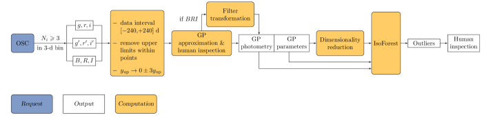
Figure 1: Workflow for the analysis. $N_{i}$ denotes the number of observations in $i$’th band. GP photometry includes 364 features: $121\times 3$ normalized fluxes and the LC flux maximum; GP parameters are 9 fitted parameters of the Gaussian process kernel and the log-likelihood of the fit.

2 The Open Supernova Catalog

The data are drawn from the Open Supernova Catalog (Guillochon et al., 2017). The catalog is constructed by combining many publicly available data sources such as the Asiago Supernova Catalog (Barbon et al., 1999), the Gaia Photometric Science Alerts (Wyrzykowski et al., 2012; Campbell et al., 2014), the Nearby Supernova Factory (Aldering et al., 2002), Pan-STARRS (Kaiser et al., 2010; Chambers et al., 2016), the SDSS Supernova Survey (Sako et al., 2018), the Sternberg Astronomical Institute Supernova Light Curve Catalogue (Tsvetkov et al., 2005), the Supernova Legacy Survey  (SNLS, Pritchet & SNLS Collaboration, 2005; Astier et al., 2006), the MASTER Global Robotic Net (Lipunov et al., 2010), the All-Sky Automated Survey for Supernovae (ASAS-SN, Holoien et al. 2019), and the intermediate Palomar Transient Factory (iPTF, Law et al. 2009; Cao et al. 2016a) among others, as well as from individual publications. It represents an open repository for supernova metadata, light curves, and spectra in an easily downloadable format. This catalog also includes some contamination from non-SN objects.

Given the large number of objects and their diverse characteristics, this catalog is ideal for our goal of automatically identifying anomalies. It incorporates data for more than $5\times 10^{4}$ SNe candidates among which $\sim$1.2$\times 10^{4}$ objects have $>$10 photometric observations and $\sim$5$\times 10^{3}$ have spectra. For comparison, SDSS supernova catalog contains only 4607 SNe candidates: 889 with measured spectra (Sako et al., 2018).

The catalog stores the data in different photometric passbands. To have a more homogeneous sample, we chose only those objects that have LCs in $BRI$ (Bessell, 1990), $g^{\prime}r^{\prime}i^{\prime}$ or $gri$ filters. The primed system $u^{\prime}g^{\prime}r^{\prime}i^{\prime}z^{\prime}$ is defined in the natural system of the USNO 1-m telescope. The SDSS magnitudes $ugriz$, however, are defined in the natural system of the SDSS 2.5-m telescope. These two systems are very similar and the coefficients of the transformation equations are quite small (Fukugita et al., 1996; Tucker et al., 2006; Smith et al., 2007). We assume that $g^{\prime}r^{\prime}i^{\prime}$ filters are close enough to $gri$ and transform $BRI$ to $gri$ (see Sect. 3.1). We require a minimum of three photometric points in each filter with a 3-day binning (Fig. 1). Our experiments show that this threshold is enough to provide a good reconstruction of the light curve — specially in cases where photometric points are not homogeneously distributed among filters. This is natural consequence of the light curve approximation procedure we adopted (Section 3.2) which takes into account the correlation between photometric bands to guide the reconstruction in sparsely populated filters. After this first cut, our sample consists of 3197 objects (2026 objects in $g^{\prime}r^{\prime}i^{\prime}$, 767 objects in $gri$, and 404 objects in $BRI$).

We downloaded the data from the GitHub page of the Astrocats project on June, 2018. The complete data set of 45162 objects is located at http://snad.space/osc/sne.tar.lzma.

3 Pre-processing

In this section we describe how to get features for ML from the OSC light curves. The pre-processing procedure includes several steps that are described in detail in the subsections below and illustrated by Fig. 1. First, we prepared the photometric data extracted from the OSC; we transformed the magnitudes to the flux units, converted the upper limits, and implemented 1-day time-binning. Then, we used the Gaussian processes to approximate the photometric observations in each filter. The objects with bad light curve approximations were removed from the further analysis. After that, we transformed the remaining light curves in $BRI$ filters to $gri$. To have a homogeneous input data, for each object we extracted its photometry in the range $[-20,+100]$ days relative to the maximum flux. We also kept the kernel parameters of the Gaussian processes. All of this together was subjected to the dimensionality reduction procedure using t-SNE method (Maaten & Hinton, 2008).

3.1 Filter transformation

In order to ensure maximum exploitation of the data at hand, we convert the Bessel’s $BRI$ into $gri$ filters using the Lupton’s (2005) transformation equations. These equations are derived by matching SDSS DR4 photometry to Peter Stetson’s published photometry for stars:

$$\left\{\begin{aligned} B&=u-0.8116\ (u-g)+0.1313\\ B&=g+0.3130\ (g-r)+0.2271\\ V&=g-0.2906\ (u-g)+0.0885\\ V&=g-0.5784\ (g-r)-0.0038\\ R&=r-0.1837\ (g-r)-0.0971\\ R&=r-0.2936\ (r-i)-0.1439\\ I&=r-1.2444\ (r-i)-0.3820\\ I&=i-0.3780\ (i-z)-0.3974\end{aligned}\right.$$ (1)

As we can see, there are several possibilities to obtain $gri$ light curves from the Bessel’s ones. Obviously, the accuracy of the transformation increases with the number of available filters. However, in the Open Supernova Catalog objects having photometry only in two filters are more numerous than those having photometry in three or four filters. Therefore, the less filters we use, the larger sample of SNe candidates we obtain. First, we tried to use only two Bessel’s filters. Prior to applying the filter transformation, we approximated the LCs with Gaussian processes (see Sect. 3.2). To evaluate the quality of transformation, with two filters only, we chose a few objects with LCs available in both, Sloan and Bessel’s filters, and compared the transformed $gri$ with the original ones. As can be seen from the Fig. 2, the results of comparison are unsatisfactory for $i$ filter. This indicated that at least one more filter had to be added in the analysis. The same test showed that three filters ($BRI$) are enough to adequately reproduce $gri$ light curves (Fig. 2). Since with 3 filters the equations become over-determined, we used the least-square method to solve Eq. 1.

Despite the fact that the transformation between the filters depends on the spectrum of an object, and Lupton’s equations are derived for stars, not for supernovae, the Fig. 2 shows quite good agreement between transformed and original light curves.

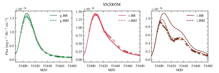
Figure 2: Light curves of SN2005M. Crosses are the observations in $gri$ filters (Ganeshalingam et al., 2010; Contreras et al., 2010; Silverman et al., 2012). Solid and dashed lines are the approximated and transformed light curves from the Bessel’s $BR$ and $BRI$ to $gri$ filters, respectively.

3.2 Light curve approximation

Traditionally, ML algorithms require a homogeneous input data matrix which, unfortunately, is not the case with supernovae. A commonly used technique to transform unevenly distributed data into an uniform grid is to approximate them with Gaussian processes (Rasmussen & Williams, 2005). Usually, each light curve is approximated by GP independently. However, in this study we use a Multivariate Gaussian Process approximation. For each object it takes into account the correlation between light curves in different bands, approximating the data by GP in all filters in a one global fit (for details see Kornilov et al. 2019, in prep.). With this technique we can reconstruct the missing parts of LC from its behaviour in other filters. For example, in Fig. 11 maximum in $g$ filter is reproduced from the $r,i$ light curves. This correlation does not rely on any physical assumptions about LC shape. As an approximation range we chose $[-20,+100]$ days. We also extrapolated the GP approximation to fill this range if needed. Once the GP approximation becomes negative, it is zeroed till infinity.

Gaussian process is based on the so-called kernel, a function describing the covariance between two observations. The kernel used in our implementation of Multivariate Gaussian Process is composed of three radial-basis functions $k_{i}(t_{1},t_{2})=\exp{\left(-\frac{(t_{2}-t_{1})^{2}}{2\,l_{i}^{2}}\right)}$, where $i$ denotes the photometric band, and $l_{i}$ are the parameters of Gaussian process to be found from the light curve approximation. These length parameters describe the characteristic time scale of correlation between observations. If the value of $l_{i}$ is too small the approximated light curve will be over-fitted and can show unrealistic oscillations. To prevent it we set a lower limit on $l_{i}$ as the maximum time interval between two neighbouring observations, but not larger than 60 days. Also, Multivariate Gaussian Process kernel includes 6 constants, three of which are unit variances of basis processes and three others describe their pairwise correlations. Totally, Multivariate Gaussian Process has 9 parameters to be fitted.

Prior to applying the GP approximation, we prepare the data (Fig. 1). First, we transform the magnitudes given by the Open Supernova Catalog to fluxes and perform all further analysis in the flux space only. Since measurements remote in time from the maximum (mainly the upper limits or host detection) could potentially affect the GP behaviour, including the main part of light curve around maximum, for each object we take only the points in the interval $[-240,+240]$ days relative to the maximum in $r,r^{\prime},R$ filter depending on the sub-sample. The Julian dates are rounded to integers. We also implement 1-day time-binning to the data.

In every bin the flux $y$ and its error $\sigma$ are derived from $n$ observations $\{y_{i},\sigma_{i}\}$ as follows (Agekian, 1972):

$$\begin{split}w_{i}&\equiv\frac{1}{\sigma_{i}^{2}},\\ w&\equiv\sum{w_{i}},\\ y&=\frac{\sum{w_{i}\,y_{i}}}{w},\\ \langle\sigma\rangle&\equiv\sqrt{\frac{\sum{w_{i}\,(y_{i}-y)^{2}}}{w\,(n-1)}},\\ \sigma_{w}&\equiv w^{-1/2},\\ \sigma&=\left\{\begin{split}&\langle\sigma\rangle,&\langle\sigma\rangle>\sigma_{w},\\ &\frac{1}{2}\left(\langle\sigma\rangle+\sigma_{w}\right),&\langle\sigma\rangle\leq\sigma_{w},\end{split}\right.\end{split}$$ (2)

where $w_{i}$ is the weight of observation, $w$ is the sum of weights, $\langle\sigma\rangle$ is the mean error, $\sigma_{w}$ is the error of the weighted mean. If the mean error is larger than the error of the weighted mean, then observation errors are probably underestimated or the object is very variable during the considered time interval. Upper limits are taken into account only if there are no detections in the bin. In this case we keep the most conservative upper limit, i.e. the one with the smallest flux.

Since for each object the OSC assembles the photometry obtained by different telescopes with different limited magnitudes, a lot of upper limits appeared in between or even simultaneously with the real detections. This could also have an undesirable impact on the Gaussian processes approximation. Therefore, for each filter we keep only those upper limits which are later than the latest real detection or earlier than the earliest real detection. Furthermore, we reassign the values of these upper limits $y_{\rm up}$: the new values are zeros with error equal to $3\times y_{\rm up}$. This is done to decrease the influence of too high upper limits on the GP approximation and to force it to vanish for very early and very late times. Some particular aspects of pre-processing are illustrated in Fig. 3.

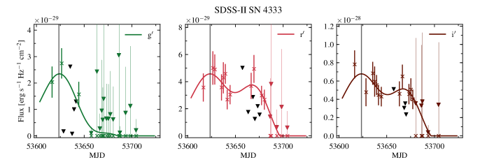
Figure 3: An example of multicolour light curve explaining the pre-processing procedure. The crosses with errorbars denote the real photometric detections. Coloured triangles are the original upper limits ($y_{\rm up}$) which are either later than the latest real detection or earlier than the earliest real detection. They are transformed into the observations with $y=0\pm 3y_{\rm up}$ (crosses with the thin errorbars). Black triangles are upper limits which are ignored. GP approximation of the crosses is shown by solid lines.

Once the Multivariate Gaussian Process approximation was done, we visually inspected the resulting light curves. Those SNe with unsatisfactory approximation were removed from the sample (mainly the objects with bad photometric quality). The remaining $BRI$ approximated light curves were then transformed to $gri$ (Sect. 3.1).

We consider the light curves in the observer frame. Since each object has its own flux scale due to the different origin and different distance, we normalized the flux vector by its maximum value. Based on the results of this approximation, for each object we extracted the kernel parameters, the log-likelihood of the fit, LC maximum and normalized photometry in the range of $[-20,+100]$ days with 1-day interval relative to the maximum. These values were used as features for the ML algorithm (Sect. 4).

Our final sample consists of 1999 objects, $\sim$30% of which have at least one spectrum in the OSC (see Fig. 4). The distribution of these objects by astrophysical types is also shown in Fig. 4. The classification is extracted from the OSC without any verification, it can be photometric or based on one spectrum only. Less than 5% of our sample have $<$20 photometric points in all three filters. The distributions of objects by redshift and by number of photometric points for the three sub-samples are shown in Figs. 5 and 6. The Fig. 5 contains only 1624 objects which significantly exceeds the number of objects with the OSC spectra. The reason for such discrepancy is that, first, the OSC collects also the photometric redshifts and, second, not all spectroscopically confirmed supernovae have the spectrum available in the public domain (for details, see Guillochon et al. 2017).

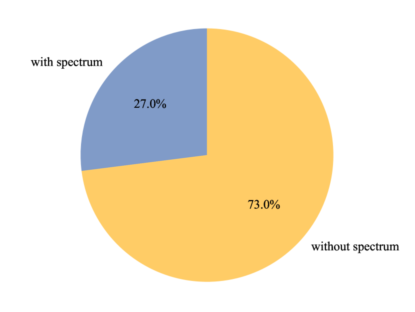
(a)

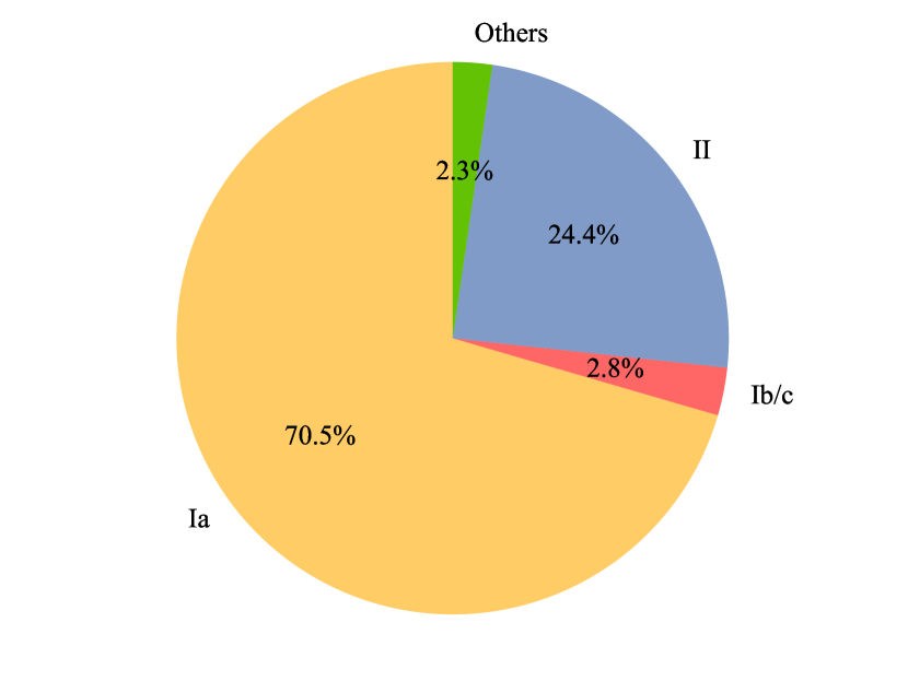
(b)

Figure 4: (a) Fraction of objects from our sample with at least one spectrum in the Open Supernova Catalog; (b) Distribution of these objects by the OSC types.

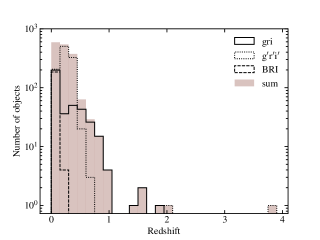
Figure 5: Distribution of objects from our sample by the redshift for three sub-samples and in total. The redshift is available for 1624 objects only.

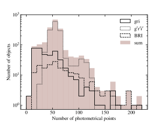
Figure 6: Distribution of objects from our sample by the number of photometric points for three sub-samples and in total.

3.3 Dimensionality Reduction

After the approximation procedure, each object has 374 features: $121\times 3$ normalized fluxes, the LC flux maximum, 9 fitted parameters of the Gaussian process kernel, and the log-likelihood of the fit.

We apply the outlier detection algorithm not only to the full data set but also to the dimensionality-reduced data. The reason for this is that the initial high dimensional feature space can be too sparse for the successful performance of the isolation forest algorithm. We applied t-SNE (Maaten & Hinton, 2008), a variation of the stochastic neighbour embedding method (Hinton & Roweis, 2003), for the dimensionality reduction of the data. In the t-SNE technique, a nonlinear dimensionality reduction mapping is obtained so as to keep distribution of distances between points undisturbed. This ensures that if a point is anomalous in the sense that it is distant from other points in the original data, it remains anomalous in the lower dimension space. As a result of the dimentionality reduction, we obtain 8 separate reduced data sets corresponding to 2 to 9 t-SNE features (dimensions). Since t-SNE is a stochastic technique we have also taken additional precautions to ensure that the resulting outlier list does not depend on the t-SNE initial random state.

4 Isolation Forest

Isolation forest (Liu et al., 2008, 2012) is an ensemble of random isolation trees. Each isolation tree is a space partitioning tree similar to the widely-known Kd-tree (Bentley, 1975). However, in contrast to the Kd-tree, a space coordinate (a feature) and a split value are selected at random for every node of the isolation tree. This algorithm leads to an unbalanced tree unsuitable for efficient spatial search. However, the tree has the following important property: a path distance between the root and the leaf is shorter on average for points distant from "normal" data. This allows us to construct enough random trees to estimate average root-leaf path distance for every data sample that we have, and then rank the data samples based on the path length. The anomaly score, defined in a range $[0,1]$, is assigned to each object (see Eq. 2 in Liu et al. 2008). Then, objects with the highest anomaly score — outliers — are selected according to the contamination level which is a hyper-parameter of the algorithm. The isolation forest algorithm is illustrated in Fig. 7.

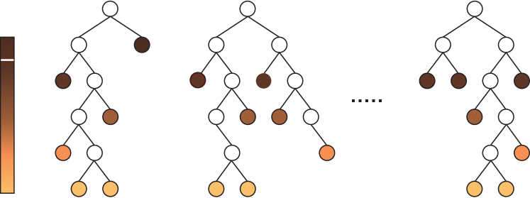
Figure 7: Isolation forest structure. Forest consists of the independent decision trees. To build a branching in a tree a random feature and a random splitting are selected. The tree is built until each object of a sample is isolated in a separate leaf — the shorter path corresponds to a higher anomaly score which is also illustrated by the colour. For each object, the measure of its normality is a function of the depths of the leaves into which it is isolated.

We run the isolation forest algorithm on 10 data sets obtained using the same photometric data (Fig. 1):

1. data set of 364 photometric characteristics ($121\times 3$ normalized fluxes, the LC flux maximum),

2. data set of 10 parameters of the Gaussian process (9 fitted parameters of the kernel, the log-likelihood of the fit),

3. 8 data sets obtained by reducing 374 features to 2–9 t-SNE dimensions (Sect. 3.3).

For each data set we obtained a list of outliers. Contamination levels were set to 1% (20 objects with highest anomaly score) for data sets A and B. For all data sets in case C we considered 2% contamination (40 objects with highest anomaly score). This larger contamination was chosen to take into account the influence of the dimensionality reduction step in the final data configuration. Given different representations of the data and the stochastic nature of the isolation forest algorithm, the same object can be assigned a different anomaly score depending on how many t-SNE dimensions are used. Thus, only those objects which were listed within the 2% contamination in at least 2 of the data sets in case C are included in Table LABEL:outliers_table and subjected to further astrophysical analysis. The distribution of objects in each of 10 data sets by anomaly score is presented in Fig. 8.

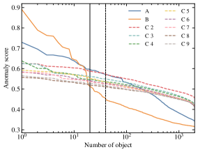
Figure 8: Distribution of objects by anomaly score in 10 data sets described in Sect. 4, C 2 – C 9 denote C data sets with 2–9 t-SNE dimensions. In each data set objects are ordered by score. Black solid and dashed lines denote 1% and 2% contamination level of outliers, respectively.

An example of the isolation forest algorithm applied to the three-dimensional reduced data set is shown in Fig. 9.

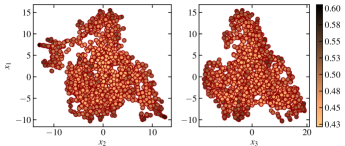
Figure 9: Three-dimensional t-SNE reduced data after application of the isolation forest algorithm. Each point represents a supernova light curve from the data set projected into the three-dimensional space with the coordinates $(x_{1},x_{2},x_{3})$. The intensity of the colour indicates the anomaly score for each object as estimated by the isolation forest algorithm. A darker color corresponds to the objects with higher anomaly scores.

5 Results

Applying the unsupervised learning to the photometric data extracted from the Open Supernova Catalog we found $\sim$100 outliers among a total of 1999 objects (Fig. 1). However, not all of them are necessary anomalies. That is why we also subject the outliers to the careful astrophysical analysis. Using publicly available sources, we collected information about each outlier and determined to which kind of astrophysical objects it belongs — given the information we could gather. Among the detected outliers there are few known cases of miss-classifications, representatives of rare classes of SNe (e.g., superluminous supernovae, 91T-like SNe Ia) and highly reddened objects. We also found that 16 anomalies classified as supernovae by Sako et al. (2018), are likely to be quasars or stars.

Light curves with GP approximation for all 1999 objects can be found at http://snad.space/osc/ and those who considered anomalous according to the criteria described in the previous section are listed in Table LABEL:outliers_table. Names and equatorial coordinates of outliers are shown in Columns 1-3; types in Column 4. CMB redshifts are presented in Column 5. Columns 6-8 contain the names and equatorial coordinates of the corresponding host galaxies. Host morphological types are displayed in Column 9. Columns 10 and 11 contain the separation between center of the host and object in angular seconds and kiloparsecs, respectively (to calculate the angular diameter distance we use a flat $\Lambda$CDM cosmology with $H_{0}=70$ km s^-1 Mpc^-1, $\Omega_{\Lambda}=0.7$). We give our comments and short description of each object in Column 12. References are in Column 13. The most interesting of these objects are described below.

5.1 Peculiar SNe Ia

Type Ia supernova is an explosion of a carbon-oxygen white dwarf that exceeds the Chandrasekhar limit either by matter accretion from a companion star or by merging with another white dwarf (Whelan & Iben, 1973; Iben & Tutukov, 1984; Webbink, 1984). SNe Ia are used as universal distance ladder since their luminosity at maximum light is approximately the same (Perlmutter et al., 1999; Riess et al., 1998). However, the class of SNe Ia is not homogeneous, for example, 91T-like supernovae are on average 0.2–0.3 mag more luminous than normal SNe Ia, have broader LCs, and different early spectrum evolution (Filippenko et al., 1992b; Blondin et al., 2012); 91bg-like supernovae are subluminous and fast-declining (Filippenko et al., 1992a); peculiar SNe Iax are spectroscopically similar to SNe Ia, but have lower maximum-light velocities and typically lower peak magnitudes (Foley et al., 2013). The presence of non-classical SNe Ia in cosmological samples may introduce a systematic bias and affect the cosmological analysis (e.g., Scalzo et al. 2012).

5.1.1 SN2002bj

SN2002bj was discovered in NGC 1821 on unfiltered CCD frames taken with the Puckett Observatory 0.60-m automated patrol telescope on 2002 February 28.06 and March 1.05 UT, and on unfiltered CCD LOTOSS images taken with the 0.8-m Katzman Automatic Imaging Telescope on February 28.2 and March 1.2 UT (Puckett et al., 2002). This supernova was a first representative of rapidly evolving events (Fig. 10). Its light curve has a rise time of $<$7 days followed by a decline of $0.25$ mag day^-1 in $B$ band and reaches a peak intrinsic brightness greater than $-18$ mag (Poznanski et al., 2010). The spectra are similar to that of a SN Ia but show the presence of helium and carbon lines. The analysis of archive data after the discovery of this object and the subsequent observations revealed other bright, fast-evolving supernovae, e.g., SN1885A, SN1939B, SN2010X, SN2015U (Kasliwal et al., 2010; Perets et al., 2011; Shivvers et al., 2016). These objects can be produced by the detonation of a helium shell on a white dwarf, ejecting a small envelope of material (Poznanski et al., 2010).

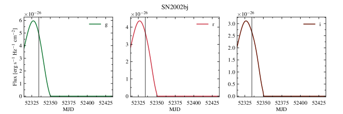
Figure 10: Light curves in $gri$ filters of peculiar SN Ia 2002bj (Poznanski et al., 2010). Solid lines are the results of our approximation by Multivariate Gaussian Process. The LCs in $gri$ filters are obtained from the Bessel’s $BRI$ by filter transformation (Sect. 3.1), thus the observations are absent on the plot. The vertical line denotes the moment of maximum in $R$ filter.

5.1.2 SN2013cv

SN2013cv was independently discovered by Zhou et al. (2013) and iPTF (Law et al., 2009) on 2013 May 1.44 UT, see Fig. 11. This peculiar supernova has large peak optical and UV luminosity and show an absence of iron absorption lines in the early spectra. Cao et al. (2016b) suggests that SN2013cv is an intermediate case between the normal and super-Chandrasekhar events.

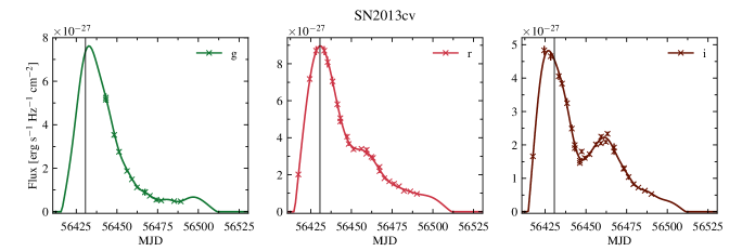
Figure 11: Light curves in $gri$ filters of peculiar SN Ia 2013cv (Cao et al., 2016b; Yaron & Gal-Yam, 2012). Solid lines are the results of our approximation by Multivariate Gaussian Process. The vertical line denotes the moment of maximum in $r$ filter.

5.1.3 SN2016bln

SN2016bln/iPTF16abc discovered by the iPTF on 2016 April l3.36 UT (Miller et al., 2016; Cenko et al., 2016) and classified by our code as outlier, belongs to the 91T-like SNe Ia subtype (see Fig. 12). The transitional and nebular spectrum of SN2016bln appear similar to the normal SN2011fe as well as to over-luminous SNe 1991T and 1999aa (Dhawan et al., 2018). Early-time observations show a peculiar rise time, non-evolving blue colour, and unusual strong $\rm C~{}II$ absorption. These features can be explained by the ejecta interaction with nearby, unbound material or/and significant ⁵⁶Ni mixing within the SN ejecta (Miller et al., 2018).

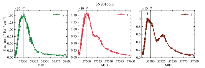
Figure 12: Light curves in $gri$ filters of 91T-like SN Ia 2016bln (Miller et al., 2018). Solid lines are the results of our approximation by Multivariate Gaussian Process. The vertical line denotes the moment of maximum in $r$ filter.

5.2 Peculiar SNe II

Type II supernovae arise from the core collapse of massive stars at the final stage of their evolution. The radius of these stars can be several hundred times greater than the solar radius, and their extremely tenuous envelopes contain large amounts of hydrogen. That is why hydrogen lines are the most prominent in the spectra of SNe II. Based on the shape of light curves Type II supernovae have historically been divided into the Type IIL (linear) and Type IIP (plateau) subtypes, however the following studies revealed a continuity in light curve slopes of Type II SNe (Anderson et al., 2014; Sanders et al., 2015a).

5.2.1 SN2013ej

Light curve of SN2013ej, discovered by the Lick Observatory Supernova Search on 2013 July 25.45 UT (Kim et al., 2013), appears intermediate between those of Type IIP and IIL supernovae (see Fig. 13). The event has a higher peak luminosity, a faster post-peak decline, and a shorter plateau phase compared to the normal Type IIP SN 1999em. The radioactive ⁵⁶Ni mass is 0.02 ${M}_{\odot}$, which is significantly lower than for typical SNe IIP (Huang et al., 2015). The source exhibits signs of substantial geometric asphericity, X-rays from persistent interaction with circumstellar material (CSM), thermal emission from warm dust (Mauerhan et al., 2017).

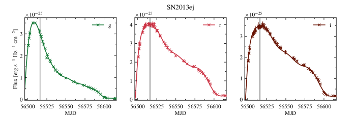
Figure 13: Light curves in $gri$ filters of peculiar SN II 2013ej (Yuan et al., 2016). Solid lines are the results of our approximation by Multivariate Gaussian Process. The vertical line denotes the moment of maximum in $r$ filter.

5.2.2 SN2016ija

This supernova was discovered on 2016 November 21.19 UT (Tartaglia et al. 2016, see Fig. 14) during one-day cadence SN search for very young transients in the nearby Universe (DLT40). Using SNID (Blondin & Tonry, 2007), it was first suggested to be an early time 91T-like SN Ia with few features and red continuum. It has been also associated to the outburst in an obscured luminous blue variable, an intermediate luminosity red transient or a luminous red nova (Blagorodnova et al., 2016). The subsequent spectroscopic follow-up revealed broad $\rm H_{\alpha}$ and calcium features, leading to a classification as a highly extinguished Type II supernova. The colour excess from the host galaxy NGC 1532 is $E(B-V)_{\rm host}=1.95\pm 0.15$ mag (Tartaglia et al., 2018). Moreover, SN2016ija is brighter than usual SNe II (see fig. 6 of Tartaglia et al. 2018).

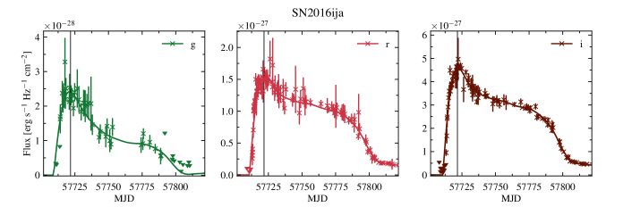
Figure 14: Light curves in $gri$ filters of peculiar SN II 2016ija (Tartaglia et al., 2018). Solid lines are the results of our approximation by Multivariate Gaussian Process. The vertical line denotes the moment of maximum in $r$ filter.

5.3 Superluminous SNe

Superluminous SNe are supernovae with an absolute peak magnitude $M<-21$ mag in any band. According to Gal-Yam (2012) SLSN can be divided into three broad classes: SLSN-I without hydrogen in their spectra, hydrogen-rich SLSN-II that often show signs of interaction with CSM, and finally, SLSN-R, a rare class of hydrogen-poor events with slowly evolving LCs, powered by the radioactive decay of ⁵⁶Ni. SLSN-R are suspected to be pair-instability supernovae: the deaths of stars with initial masses between 140 and 260 solar masses.

In our outlier list in Table LABEL:outliers_table there are four SLSN: SDSS-II SN 17789, SN2015bn, PTF10aagc, SN2213-1745.

5.3.1 SN2213-1745

SN2213-1745 was discovered at $z=2.046$ by the Canada-France-Hawaii Telescope Legacy Survey (Fig. 15). It belongs to the SLSN-R events. Cooke et al. (2012) suggested that SN 2213-1745 may be powered by the radiative decay of a 4–7 $M_{\odot}$ of synthesised ⁵⁶Ni, and implied a progenitor with an estimated initial mass of $\sim$250 $M_{\odot}$.

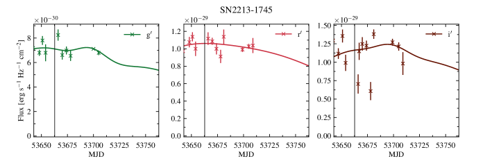
Figure 15: Light curves in $g^{\prime}r^{\prime}i^{\prime}$ filters of superluminous supernova SN2213-1745 (Cooke et al., 2012). Solid lines are the results of our approximation by Multivariate Gaussian Process. The vertical line denotes the moment of maximum in $r^{\prime}$ filter.

5.3.2 PTF10aagc

The high peak luminosity ($L_{\rm bol,peak}=10^{43.7}$ erg s^-1) and the absence of hydrogen lines in early spectrum allowed to attribute PTF10aagc to SLSN-I (De Cia et al. 2018, see Fig. 16). However, the latter spectra revealed a broad $\rm H_{\alpha}$ and the corresponding weak, but detected $\rm H_{\beta}$ (Yan et al., 2015). This particularity makes PTF10aagc clearly distinct from others SLSN-I. Such spectral behaviour can be explained by interaction between SLSN-I ejecta and a H-rich circumstellar material at late times (Yan et al., 2015). The host of PTF10aagc is bright and shows clear morphological structure suggesting a possible ongoing merger (Perley et al., 2016).

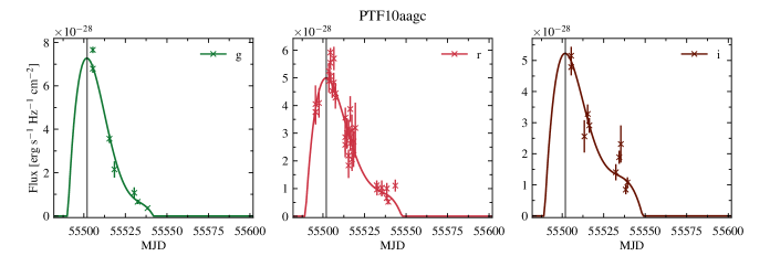
Figure 16: Light curves in $gri$ filters of superluminous supernova PTF10aagc (De Cia et al., 2018). Solid lines are the results of our approximation by Multivariate Gaussian Process. The vertical line denotes the moment of maximum in $r$ filter.

5.4 Misclassified objects

5.4.1 SN2006kg

SN2006kg was first classified as a possible Type II SN (Bassett et al. 2006, see Fig. 17). It is also appeared as Type II spectroscopically confirmed supernova in table 6 of Sako et al. (2008). However, further analysis of 3.6-m New Technology Telescope spectrum revealed that SN2006kg is an active galactic nucleus (Östman et al., 2011; Sako et al., 2018). It is interesting that SN2006kg continues to appear as supernova in host studies (Hakobyan et al., 2012) and was even in a set of 12 well-observed events that were used as Type II supernova templates (Okumura et al., 2014). The object is not in the WISE AGN Catalog (Assef et al., 2018) that consists of $>$20 millions AGN candidates.

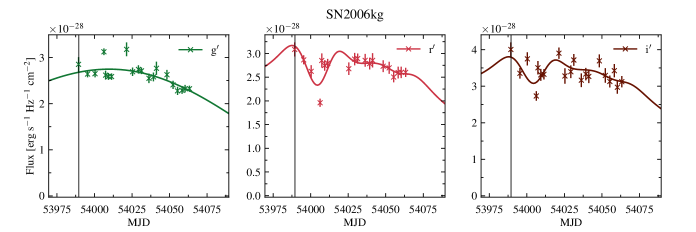
Figure 17: Light curves in $g^{\prime}r^{\prime}i^{\prime}$ filters of active galactic nucleus SN2006kg (Sako et al., 2018). Solid lines are the results of our approximation by Multivariate Gaussian Process. The vertical line denotes the moment of maximum in $r^{\prime}$ filter.

5.4.2 Gaia16aye

Gaia16aye (Bakis et al., 2016) is an object with the most non-SN-like behavior among our set of outliers (Fig. 18). In Wyrzykowski et al. (2016) it was reported that Gaia16aye is a binary microlensing event — gravitational microlensing of binary systems — the first ever discovered towards the Galactic Plane.

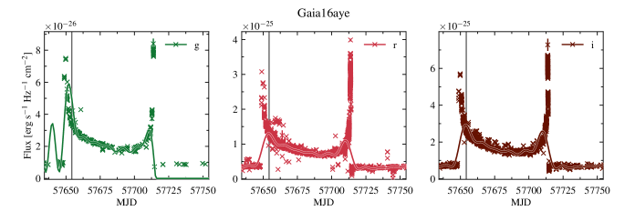
Figure 18: Light curves in $gri$ filters of binary microlensing event Gaia16aye (http://gsaweb.ast.cam.ac.uk/alerts/alert/Gaia16aye/followup). Solid lines are the results of our approximation by Multivariate Gaussian Process. The vertical line denotes the moment of maximum in $r$ filter.

5.4.3 Possible misclassified objects

Our analysis also reveals that 16 objects classified as pSN by  Sako et al. 2018, where a prefix "p" indicates a purely photometric type, are likely to be stars or quasars. First, we do not find any signature of supernovae on the corresponding multicolour light curves. Then, according to SDSS DR15 type of SDSS-II SN 5314, SDSS-II SN 14170, SDSS-II SN 15565, SDSS-II SN 13725, SDSS-II SN 13741, SDSS-II SN 19699, SDSS-II SN 18266, SDSS-II SN 4226, SDSS-II SN 2809, SDSS-II SN 6992 is denoted as STAR. Moreover, all these objects can be found in Pan-STARRS Catalog with Pan-STARRS magnitudes equal or even brighter than those on the corresponding light curves.

The other objects SDSS-II SN 1706, SDSS-II SN 17756, SDSS-II SN 17339, SDSS-II SN 17509, SDSS-II SN 4652, SDSS-II SN 19395 have a BOSS (Smee et al., 2013) spectrum with class "QSO" and have high redshifts (see Table LABEL:outliers_table)

6 Conclusions

The development of large sky surveys has led to a discovery of a huge number of supernovae and supernova candidates. Among the SNe discovered every year, only 10% have spectroscopic confirmation. The amount of astronomical data increases dramatically with time and is already beyond human capabilities. The astronomical community already has dozens of thousands of SN candidates, and LSST survey (LSST Science Collaboration et al., 2009) will discover over ten million supernovae in the forthcoming decade. Only a small fraction of them will receive a spectroscopic confirmation. This motivates a considerable effort in photometric classification of supernovae by types using machine learning algorithms. There is, however, another aspect of the problem: any large photometric SN database would suffer from the non-SN contamination (novae, kilonovae, GRB afterglows, AGNs, etc.). Moreover, the database will inevitably contain the astronomical objects with unusual physical properties — anomalies. Finding such objects and studying them in detail is very important and constitutes the main goal of this paper.

The analysis presented here is based on the photometric data extracted from the Open Supernova Catalog (Guillochon et al., 2017). The use of real data allows us to reveal a lot of caveats in observations at the pre-pocessing stage – many of which are not normally present in the simulated data. After pre-processing, we obtain 1999 SNe with light curves either in $gri$ or in $g^{\prime}r^{\prime}i^{\prime}$ or in $BRI$ filters approximated by Gaussian processes. We consider 10 different data sets: one that includes the approximated photometric observations (A), another with the parameters of Gaussian process only (B) and 8 data sets were the information in GP photometry and GP parameters were summarised via dimensionality reduction using t-SNE (dimension varying from 2 to 9, case C).

We apply the isolation forest algorithm to all data sets, considering a 1% contamination for cases A/B and 2% contamination for all data sets in case C. We visually checked all objects identified in cases A and B. We also checked all the objects which were identified as anomalous in at least 2 of the data sets in case C. As a result, we find $\sim$100 outliers, 40 from cases A/B and 60 which were identified in at least two data sets of case C. Among these, 19 objects were identified by both strategies, with and without dimensionality reduction. Our final validation analysis resulting in 81 objects which were carefully studied with the use of publicly available information. Among these there are four superluminous supernovae (SDSS-II SN 17789, SN2015bn, PTF10aagc, SN2213-1745), non-classical Type Ia SNe (91T-like SNe 2016bln, PS15cfn, SNLS-03D1cm; peculiar SN2002bj and SN2013cv), two unusual Type II SNe which anomalous multicolour light curve behaviour can be due to the environment (SN2013ej, SN2016ija), one AGN – SN2006kg, and one binary microlensing event Gaia16aye. We also find that 16 anomalies classified as supernovae by Sako et al. (2018), which are likely to be stars (SDSS-II SN 5314, SDSS-II SN 14170, SDSS-II SN 15565, SDSS-II SN 13725, SDSS-II SN 13741, SDSS-II SN 19699, SDSS-II SN 18266, SDSS-II SN 4226, SDSS-II SN 2809, SDSS-II SN 6992) or quasars (SDSS-II SN 1706, SDSS-II SN 17756, SDSS-II SN 17339, SDSS-II SN 17509, SDSS-II SN 4652, SDSS-II SN 19395). However, without careful spectral analysis it is difficult to distinguish a high-redshift supernova against a background galaxy or from quasar activity. As a confirmation of the robustness of the pipeline used here, we note that of the 9 objects identified as outliers in all data sets of case C, 5 are miss-classifications and 1 is an extreme case of bad photometry.

In summary, the isolation forest analysis identified 81 potentially interesting objects, from which 27 (33%) where confirmed to be non-SN events or representatives of the rare SN classes. Found anomalies correspond to 1.4% of the original data set of $\sim$2000 objects which was identified demanding significantly less resources than a manual search would entail. Among these objects, we report for the first time the 16 star/quasar-like objects misclassified as SNe.

It is important to note that this results are not expected to be complete. For example, there are known SLSN which were not identified as outliers in our search, as well as 1 object (SN1000+0216) at very high redshift which was identified as anomalous in only 1 of the data sets for case C — and consequently was not included in our final list. This is a natural consequence of the pre-processing analysis we chose to adopt, where the objects are mainly characterised by their light curve shape (all photometric features were normalised). In this context, differences in intrinsic brightness only marginally affect our final results. Another source of false negatives can be traced back to GP approximations, the typical example being Gaia16aye (Fig. 18). From a visual inspection of its observed photometric points this objects is obviously not a SN. However, it appeared only in 3 of the 8 possible data sets in case C. A more detailed analysis of its GP approximation (solid line in Fig. 18), reveals that the information input to the ML model was much smoother than one would expect. As a consequence, the algorithm struggles to separate it from other slow declining events.

Nevertheless, the above results provide clear evidence of the effectiveness of automated anomaly detection algorithms for photometric SN light curve analysis. In this work we used data from the OSC in order to provide a proof of concept. Although this is not a big data sample, it does allow us to search for independent information in the literature on which we could confirm our findings. This approach to the analysis of photometric light curves will be paramount for future astronomical surveys like LSST, which will not be able to afford a manual research or the possibility to overlook interesting objects deviating from the bulk of the data — where the most interesting physics resides.

The code of this work and the data are available at
http://snad.space/osc/.

Appendix A Table with outliers

Table 1: List of outliers and their hosts

Name

$\alpha$

$\delta$

Typea

zCMB

Host name

Host $\alpha$

Host $\delta$

Host typeb

Sep. (”)c

Sep. (kpc)c

Commentsd

References

Outliers found in 8 data sets with different dimensionality reduction

SDSS-II SN 13112†

01:09:29.89

$-$01:05:18.3

?SN II

SDSS J010929.89-010518.3

01:09:29.89

$-$01:05:18.3

pSN II in Sako et al. (2018); SDSS DR15 host photoZ (KD-tree method) $0.755\pm 0.234$

Sako et al. (2018)

SDSS-II SN 13461

23:03:39.48

$+$00:12:49.9

?SN II

SDSS J230339.49+001249.7

23:03:39.49

$+$00:12:49.8

pSN II in Sako et al. (2018); SDSS DR15 host photoZ (KD-tree method) $0.735\pm 0.080$

Sako et al. (2018)

SDSS-II SN 5314†

20:21:17.85

$+$00:41:04.3

?SN II/?Star

SDSS J202117.84+004104.2

20:21:17.84

$+$00:41:04.2

pSN II in Sako et al. (2018); host classified as star by SDSS DR15

Sako et al. (2018)

SN2016fbo⋆

01:01:35.54

$+$17:06:04.3

SN Ia

0.030

GALEXASC J010135.75+170604.9

01:01:35.77

$+$17:06:04.1

3.3

1.98

LC in the Open Supernova Catalog has a bad quality

Foley et al. (2018)

SDSS-II SN 14170†

01:46:33.15

$+$00:51:05.7

?SN II/?Star

SDSS J014633.15+005105.6

01:46:33.15

$+$00:51:05.6

pSN II in Sako et al. (2018); host classified as star by SDSS DR15

Sako et al. (2018)

SDSS-II SN 1706†

00:02:58.11

$-$01:01:27.8

?SN II/QSO

SDSS J000258.10-010127.8

00:02:58.10

$-$01:01:27.8

pSN II in Sako et al. (2018); according to SDSS DR15 host has BOSS spectrum with $z=1.551$, class = QSO broadline

Sako et al. (2018)

LSQ13dpa†

11:01:12.91

$-$05:50:52.6

SN II

0.023

LCSB S1492O

11:01:12.46

$-$05:50:46.0

S

9.4

4.37

Spectroscopically confirmed as SN II using a near-infrared spectrum (range 800-2500 nm)

Hsiao et al. (2013)

SDSS-II SN 17756†

01:08:10.42

$-$00:16:36.9

?SN II/QSO

SDSS J010810.43-001636.9

01:08:10.43

$-$00:16:37.0

pSN II in Sako et al. (2018); host classified as star by SDSS DR15, however, it has a BOSS spectrum with $z=1.997$, class = QSO broadline

Sako et al. (2018)

SDSS-II SN 15565

01:00:27.12

$+$00:35:23.6

?SN II/?Star

SDSS J010027.10+003523.5

01:00:27.10

$+$00:35:23.5

pSN II in Sako et al. (2018); host classified as star by SDSS DR15

Sako et al. (2018)

Outliers found in 7 data sets with different dimensionality reduction

SN2005ho⋆

00:59:24.10

$+$00:00:09.3

SN Ia

0.062

PGC 1154577

00:59:24.10

$+$00:00:09.4

Sm/Im

0.1

0.12

In JLA cosmological sample (Betoule et al., 2014), not in Pantheon (Scolnic et al., 2018)

Betoule et al. (2014)

SN2016ija

04:12:07.62

$-$32:51:10.9

SN II

0.003

NGC 1532

04:12:04.33

$-$32:52:27.2

Sbc

86.8

5.39

Highly obscured SN II ($E(B-V)_{\rm host}=1.95\pm 0.15$ mag)

Tartaglia et al. (2018)

SDSS-II SN 2050†

20:54:41.52

$-$00:13:33.2

Unknown

SDSS J205441.53-001333.1

20:54:41.53

$-$00:13:33.2

Unknown object in Sako et al. (2018) and SN II in the Open Supernova Catalog with reference to Sako et al. (2018)

Sako et al. (2018)

SDSS-II SN 17339†

02:31:22.22

$+$00:23:09.6

?SN II/QSO

SDSS J023122.22+002309.5

02:31:22.22

$+$00:23:09.5

pSN II in Sako et al. (2018); host classified as star by SDSS DR15, however, it has a BOSS spectrum with $z=1.132$, class = QSO

Sako et al. (2018)

Outliers found in 6 data sets with different dimensionality reduction

SN2007jm⋆,†

21:55:38.59

$-$00:10:36.3

SN IIn

0.090

SDSS J215538.80-001034.1

21:55:38.80

$-$00:10:34.2

3.8

6.36

According to SDSS DR15 host has BOSS spectrum with $z=0.091$, class = galaxy starforming

Bassett et al. (2007); Sako et al. (2018)

SNLS-06D3gx

14:17:03.23

$+$52:56:10.5

SN Ia

0.761

SDSS J141703.21+525616.1

14:17:03.21

$+$52:56:16.1

5.6

41.31

In JLA cosmological sample (Betoule et al., 2014), not in Pantheon (Scolnic et al., 2018)

Betoule et al. (2014)

SDSS-II SN 13725

21:06:55.01

$+$00:53:44.9

?SN II/?Star

SDSS J210655.01+005344.8

21:06:55.01

$+$00:53:44.9

pSN II in Sako et al. (2018); host classified as star by SDSS DR15

Sako et al. (2018)

SN2016ixf

10:39:44.56

$+$15:02:04.8

SN Ia

0.067

SDSS J103944.53+150204.7

10:39:44.53

$+$15:02:04.8

0.4

0.56

Cikota et al. (2016); Foley et al. (2018)

SN2006ob

01:51:48.14

$+$00:15:47.9

SN Ia

0.059

UGC 1333

01:51:48.51

$+$00:15:49.8

Sa

5.9

6.69

In JLA (Betoule et al., 2014) and Pantheon (Scolnic et al., 2018) cosmological samples

Betoule et al. (2014)

SDSS-II SN 17509

00:19:18.93

$+$01:08:14.3

?SN II/QSO

SDSS J001918.93+010814.2

00:19:18.93

$+$01:08:14.2

pSN II in Sako et al. (2018); host classified as star by SDSS DR15, however, it has a BOSS spectrum with $z=2.031$, class = QSO

Sako et al. (2018)

Outliers found in 5 data sets with different dimensionality reduction

SDSS-II SN 4330

01:44:35.82

$-$00:10:57.4

?SN II

SDSS J014435.82-001057.3

01:44:35.82

$-$00:10:57.4

pSN II in Sako et al. (2018); SDSS DR15 host photoZ (KD-tree method) $0.732\pm 0.076$

Sako et al. (2018)

SN2005ll

22:28:06.87

$-$01:07:41.4

SN Ia

0.241

SDSS J222806.92-010742.1

22:28:06.92

$-$01:07:42.1

1.0

3.90

According to SDSS DR15 host has BOSS spectrum with $z=0.242$, class = galaxy starforming

Sako et al. (2018)

SDSS-II SN 13741

20:48:00.40

$-$01:02:49.5

?SN II/?Star

SDSS J204800.39-010249.4

20:48:00.39

$-$01:02:49.5

pSN II in Sako et al. (2018); host classified as star by SDSS DR15

Sako et al. (2018)

SDSS-II SN 17292†

23:31:23.77

$+$00:37:45.6

?SN II

SDSS J233123.77+003745.4

23:31:23.77

$+$00:37:45.5

pSN II in Sako et al. (2018); SDSS DR15 host photoZ (KD-tree method) $0.595\pm 0.163$

Sako et al. (2018)

SN2006kg

01:04:16.98

$+$00:46:08.9

AGN

0.230

SDSS J010416.98+004608.7

01:04:16.98

$+$00:46:08.8

Basing on NTT spectrum classified as AGN by Östman et al. (2011); according to SDSS DR15 host has BOSS spectrum with $z=0.231$, class = galaxy starburst

Sako et al. (2018)

Outliers found in 4 data sets with different dimensionality reduction

SDSS-II SN 4652

02:29:49.69

$-$00:40:11.4

?SN II/QSO

SDSS J022949.69-004011.3

02:29:49.69

$-$00:40:11.4

pSN II in Sako et al. (2018); according to SDSS DR15 host has BOSS spectrum with $z=0.673$, class = QSO

Sako et al. (2018)

SN2002bj

05:11:46.41

$-$15:08:10.8

SN Ia pec/SN Ib pec

0.012

NGC 1821

05:11:46.11

$-$15:08:04.9

Im

7.3

1.80

Bright, fast-evolving supernova with low-mass ejecta, helium and carbon lines in spectra

Poznanski et al. (2010)

SDSS-II SN 13589†

21:48:02.39

$-$00:07:07.5

?SN II

SDSS J214802.31-000710.0

21:48:02.31

$-$00:07:10.1

pSN II in Sako et al. (2018); SDSS DR15 host photoZ (KD-tree method) $0.199\pm 0.032$

Sako et al. (2018)

SDSS-II SN 13291

20:04:11.38

$-$00:32:01.1

?SN II

SDSS J200411.38-003200.9

20:04:11.38

$-$00:32:01.0

pSN II in Sako et al. (2018); SDSS DR15 host photoZ (KD-tree method) $0.425\pm 0.119$

Sako et al. (2018)

SN2213-1745

22:13:39.97

$-$17:45:24.5

SLSN-R

2.046

Cooke et al. (2012)

SN2017mf

14:16:31.00

$+$39:35:12.0

SN Ia

0.026

NGC 5541

14:16:31.80

$+$39:35:20.7

Sb

12.7

6.64

Foley et al. (2018)

SN2017yh

17:52:06.25

$+$21:33:58.3

SN Ia

0.020

IC 1269

17:52:05.86

$+$21:34:09.0

Sbc

12.0

4.86

Foley et al. (2018)

SN2013cv

16:22:43.19

$+$18:57:35.0

SN Ia pec

0.036

SDSS J162243.02+185733.8

16:22:43.02

$+$18:57:33.8

2.7

1.93

Large peak optical and UV luminosity, absence of iron absorption lines in the early spectra

Cao et al. (2016b)

SN2006pt⋆

02:27:16.17

$-$00:23:36.5

SN Ia

0.298

SDSS J022716.08-002335.6

02:27:16.08

$-$00:23:35.6

1.6

7.21

According to SDSS DR15 host has BOSS spectrum with $z=0.299$, class = galaxy starforming

Sako et al. (2018)

SDSS-II SN 2661

23:32:49.80

$+$00:05:50.0

SN II

0.191

SDSS J233249.88+000549.2

23:32:49.88

$+$00:05:49.2

1.4

4.59

Sako et al. (2018)

SDSS-II SN 20266

00:31:13.40

$-$00:07:08.7

?SN II

pSN II in Sako et al. (2018)

Sako et al. (2018)

Outliers found in 3 data sets with different dimensionality reduction

SDSS-II SN 12868

21:29:40.40

$-$00:01:38.8

?SN II

SDSS J212940.40-000138.9

21:29:40.40

$-$00:01:39.0

pSN II in Sako et al. (2018); SDSS DR15 host photoZ (KD-tree method) $0.688\pm 0.167$

Sako et al. (2018)

SDSS-II SN 19699

02:02:11.76

$+$00:13:46.3

?SN II/?Star

SDSS J020211.76+001346.2

02:02:11.76

$+$00:13:46.2

pSN II in Sako et al. (2018); host classified as star by SDSS DR15

Sako et al. (2018)

SDSS-II SN 16302

22:07:04.15

$+$00:11:00.6

?SN Ia

22:07:04.11

$+$00:10:58.9

pSN II in Sako et al. (2018); host photoZ $0.185\pm 0.015$ (Smith et al., 2012)

Sako et al. (2018)

SDSS-II SN 15745

02:48:49.91

$-$00:06:27.1

?SN Ia

SDSS J024849.89-000626.6

02:48:49.89

$-$00:06:26.7

pSN Ia in Sako et al. (2018); SDSS DR15 host photoZ (KD-tree method) $0.657\pm 0.074$

Sako et al. (2018)

Gaia16aye⋆

19:40:01.10

$+$30:07:53.4

ULENS, CV

MW

Binary microlensing event

Bakis et al. (2016)

PS1-1000007

02:23:30.71

$-$04:38:10.8

SN Ia

0.137

SDSS J022330.91-043810.6

02:23:30.91

$-$04:38:10.7

3.0

7.25

Rest et al. (2014)

SN2006ne

01:13:37.84

$+$00:25:26.0

SN Ia

0.046

SDSS J011337.58+002525.5

01:13:37.58

$+$00:25:25.5

S

3.9

3.55

According to SDSS DR15 host has BOSS spectrum with $z=0.047$, class = galaxy starforming

Sako et al. (2018)

SDSS-II SN 19504

00:54:39.68

$-$00:25:23.9

SN II

0.214

SDSS J005439.88-002526.3

00:54:39.88

$-$00:25:26.3

3.8

13.36

Sako et al. (2018)

SDSS-II SN 18266

03:15:24.35

$-$00:50:54.0

?SN II/?Star

SDSS J031524.34-005053.9

03:15:24.34

$-$00:50:54.0

pSN II in Sako et al. (2018); host classified as star by SDSS DR15

Sako et al. (2018)

PS15cfn

21:59:21.97

$-$21:07:10.7

91T-like

0.109

GALEXASC J215922.04-210713.3

21:59:22.00

$-$21:07:13.5

2.8

5.63

Foley et al. (2018)

SDSS-II SN 15048

02:54:57.10

$-$00:00:18.6

?SN Ia

pSN Ia in Sako et al. (2018)

Sako et al. (2018)

Outliers found in 2 data sets with different dimensionality reduction

SN2006ej

00:38:59.77

$-$09:00:56.6

SN Ia

0.020

IC 1563

00:39:00.24

$-$09:00:52.4

S0

8.1

3.30

In JLA (Betoule et al., 2014) and Pantheon (Scolnic et al., 2018) cosmological samples

Betoule et al. (2014)

SDSS-II SN 18391

02:22:42.43

$+$00:25:05.0

?Unknown/?Star

SDSS J022242.43+002504.8

02:22:42.43

$+$00:25:04.9

Unknown object in Sako et al. (2018); host classified as star by SDSS DR15

Sako et al. (2018)

SN1996ai

13:10:58.13

$+$37:03:35.4

SN Ia

0.004

NGC 5005

13:10:56.31

$+$37:03:32.2

Sbc

22.0

1.82

Highly reddened SN Ia ($E(B-V)_{\rm host}=1.69\pm 0.10$ mag)

Jha et al. (2007); Wang et al. (2008)

SN2016ayg

07:30:17.40

$+$25:01:56.0

SN Ia

0.043

SDSS J073017.25+250153.5

07:30:17.26

$+$25:01:53.5

3.1

2.66

Foley et al. (2018)

SDSS-II SN 4226

23:40:41.66

$-$00:54:21.2

?SN II/?Star

SDSS J234041.66-005421.3

23:40:41.66

$-$00:54:21.3

pSN II in Sako et al. (2018); host classified as star by SDSS DR15

Sako et al. (2018)

SN2005jw

20:40:19.25

$-$00:00:25.8

SN Ia

0.380

SDSS J204019.14-000022.8

20:40:19.14

$-$00:00:22.9

Sbc/Sc

3.3

17.37

In JLA (Betoule et al., 2014) and Pantheon (Scolnic et al., 2018) cosmological samples

Zheng et al. (2008); Betoule et al. (2014)

SN2016bln⋆

13:34:45.49

$+$13:51:14.3

91T-like

0.024

NGC 5221

13:34:55.91

$+$13:49:57.1

Sb

170.3

82.41

Peculiar rise time, non-evolving blue colour, unusual strong $\rm C~{}II$ absorption

Foley et al. (2018)

SN2016bmc

19:10:37.33

$+$37:39:17.0

SN Ia

0.028

UGC 11409

19:10:37.51

$+$37:39:18.9

S

2.9

1.61

Foley et al. (2018)

SDSS-II SN 2093

22:36:36.28

$-$00:12:47.0

?SN II

pSN II in Sako et al. (2018)

Sako et al. (2018)

SDSS-II SN 17317

01:29:59.18

$-$00:38:05.4

?SN II

SDSS J012959.31-003800.3

01:29:59.31

$-$00:38:00.3

Sbc

zSN II in Sako et al. (2018); according to SDSS DR15 host has BOSS spectrum with $z=0.118$, class = starforming galaxy

Sako et al. (2018)

SNLS-03D1cm

02 24 55.27

$-$04 23 03.4

91T-like

0.870

[HSP2005] J022455.28-042303.68

02:24:55.28

$-$04:23:03.7

0.3

2.59

Peculiar Type Ia SN with the stretch-related parameter $X_{1}=4.54$

Guy et al. (2010); Bazin et al. (2011)

SDSS-II SN 17789

01:29:16.13

$+$00:42:37.9

SLSN

According to table 2 of Sako et al. (2018) SN has 4 spectra

Sako et al. (2018)

SN2015bn

11:33:41.57

$+$00:43:32.2

SLSN-I

0.114

SDSS J113341.53+004333.2

11:33:41.53

$+$00:43:33.3

1.3

2.59

Hydrogen-poor superluminous supernova

Le Guillou et al. (2015); Nicholl et al. (2016)

SDSS-II SN 2809†

03:33:27.41

$+$00:16:10.7

?SN II/?Star

SDSS J033327.41+001610.7

03:33:27.41

$+$00:16:10.7

pSN II in Sako et al. (2018); host classified as star by SDSS DR15

Sako et al. (2018)

Outliers found in a data set of 364 photometric characteristics ($121\times 3$ normalized fluxes and the LC flux maximum)

SDSS-II SN 18228

22:45:49.70

$-$00:15:54.9

?SN II

pSN II in Sako et al. (2018)

Sako et al. (2018)

SDSS-II SN 18733

01:22:42.61

$-$00:02:48.4

?SN II

pSN II in Sako et al. (2018)

Sako et al. (2018)

SDSS-II SN 19047

21:43:18.71

$+$00:32:21.7

?SN II

SDSS J214318.74+003219.8

21:43:18.74

$+$00:32:19.9

zSN II in Sako et al. (2018); according to SDSS DR15 host has BOSS spectrum with $z=0.412$, class = galaxy starburst

Sako et al. (2018)

SDSS-II SN 19395

02:44:37.90

$+$00:46:32.1

?SN II/QSO

SDSS J024437.89+004631.9

02:44:37.89

$+$00:46:32.0

pSN II in Sako et al. (2018); according to SDSS DR15 host has BOSS spectrum with $z=1.318$, class = QSO

Sako et al. (2018)

SDSS-II SN 6992

22:10:25.09

$+$00:00:02.7

?SN II/?Star

SDSS J221025.08+000002.5

22:10:25.08

$+$00:00:02.5

pSN II in Sako et al. (2018); host classified as star by SDSS DR15

Sako et al. (2018)

SN2005mp

01:04:45.68

$+$00:03:20.2

SN Ia

0.272

Host identified by Sako et al. 2018 (SDSS J010445.51+000320.8) has BOSS spectrum with $z=0.952$ that is different from SN redshift

Ganeshalingam et al. (2013); Sako et al. (2018)

SN2013ab†

14:32:44.49

$+$09:53:12.3

SN IIP

0.006

NGC 5669

14:32:43.80

$+$09:53:28.8

Scd

19.4

2.40

The light curve and spectra suggest that the supernova is a normal Type IIP event, although with a steeper decline during the plateau relative to other archetypal SNe of similar brightness

Bose et al. (2015a)

SN1999gi

10:18:16.66

$+$41:26:28.2

SN IIP

0.002

NGC 3184

10:18:16.99

$+$41:25:27.8

Sc

60.5

2.51

Leonard et al. (2002)

Outliers found in a data set of 10 Gaussian process parameters (9 fitted parameters of the kernel and the log-likelihood of the fit)

PTF10aagc

09:39:56.93

$+$21:43:16.9

SLSN-I

0.207

SDSS J093956.91+214317.1

09:39:56.91

$+$21:43:17.1

0.3

1.16

SLSN-I with hydrogen in late spectra; host morphological structure suggests a possible ongoing merger

Perley et al. (2016); De Cia et al. (2018)

SN2006T

09:54:30.21

$-$25:42:29.3

SN IIb

0.008

NGC 3054

09:54:28.61

$-$25:42:12.4

Sbc

27.4

4.51

Monard (2006); Stritzinger et al. (2018)

SN2010bb

10:44:38.23

$+$57:48:40.0

SN Ia

0.118

SDSS J104438.19+574839.8

10:44:38.19

$+$57:48:39.8

0.4

0.80

Rest et al. (2014)

SN2013ej

01:36:48.16

$+$15:45:31.0

SN IIP/SN IIL

0.002

NGC 628

01:36:41.77

$+$15:47:00.5

Sc

128.5

5.32

LC is intermediate between those of Type IIP and IIL SNe

Bose et al. (2015b); Huang et al. (2015); Mauerhan et al. (2017)

SNLS-04D2gb

10:02:22.67

$+$01:53:39.0

SN Ia

0.452

SDSS J100222.66+015339.2

10:02:22.66

$+$01:53:39.2

0.2

1.44

In JLA (Betoule et al., 2014) and Pantheon (Scolnic et al., 2018) cosmological samples; host classified as star by SDSS DR15

Betoule et al. (2014)

SNLS-05D2mp

09:59:08.63

$+$02:12:14.4

SN Ia

0.355

In JLA (Betoule et al., 2014) and Pantheon (Scolnic et al., 2018) cosmological samples

Betoule et al. (2014)

SNLS-06D2ag

10:01:43.36

$+$01:51:37.1

SN Ia

0.310

SDSS J100143.26+015135.4

10:01:43.26

$+$01:51:35.4

2.3

10.33

Guy et al. (2010); Ganeshalingam et al. (2013)

SNLS-06D3cn

14:19:25.85

$+$52:38:27.5

SN Ia

0.232

SDSS J141925.79+523825.9

14:19:25.79

$+$52:38:25.9

1.7

6.25

Guy et al. (2010)

SN1999cc

16:02:42.03

$+$37:21:34.4

SN Ia

0.032

NGC 6038

16:02:40.55

$+$37:21:34.2

Sbc

17.6

11.28

In JLA (Betoule et al., 2014) and Pantheon (Scolnic et al., 2018) cosmological samples

Betoule et al. (2014)

SN2002aw

16:37:29.06

$+$40:52:50.3

SN Ia

0.026

2MFGC 13321

16:37:29.22

$+$40:52:48.2

Sb

2.8

1.45

Ganeshalingam et al. (2013)

SN2002eb

22:19:05.24

$+$24:35:39.8

SN Ia

0.026

PGC 68560

22:19:06.29

$+$24:35:53.4

Sb

19.7

10.33

Ganeshalingam et al. (2013)

SN2004dt

02:02:12.77

$-$00:05:51.5

SN Ia

0.019

NGC 799

02:02:12.30

$-$00:06:02.6

Sa

13.1

5.07

Spectral subtype: high velocity (HV, Wang et al. 2009), broad line (BL, Branch et al. 2006)

Folatelli et al. (2013)

SN2009bw

03:56:06.92

$+$72:55:40.9

SN IIP

0.004

UGC 2890

03:56:04.44

$+$72:55:18.5

Sdm

24.9

2.06

Luminosity drop from the photospheric to the nebular phase is one of the fastest ever observed, $\sim$2.2 mag in $\sim$13 days

Inserra et al. (2012); Rodríguez et al. (2014)

a Type of the source. A prefix "?" means that the source is not confirmed spectroscopically.

b Simbad host galaxy morphological type.

c Separation of the source from the center of its host galaxy.

d If classification is made by Sako et al. 2018: a prefix "p" (pSN) indicates a purely photometric type, a prefix "z" (zSN) indicates that a redshift is measured from its candidate host galaxy and the classification uses that redshift as a prior.

⋆ The object is also found in a data set of 10 Gaussian process parameters (9 fitted parameters of the kernel and the log-likelihood of the fit).

† The object is also found in a data set of 364 photometric characteristics ($121\times 3$ normalized fluxes and the LC flux maximum).

References

- Agekian (1972) Agekian T., 1972, Fundamentals of the theory of errors for astronomers and physicists. Nauka, Moscow
- Aldering et al. (2002) Aldering G., et al., 2002, in SPIE Conference Series. pp 61–72
- Anderson et al. (2014) Anderson J. P., et al., 2014, ApJ, 786, 67
- Assef et al. (2018) Assef R. J., Stern D., Noirot G., Jun H. D., Cutri R. M., Eisenhardt P. R. M., 2018, The Astrophysical Journal Supplement Series, 234, 23
- Astier et al. (2006) Astier P., et al., 2006, A&A, 447, 31
- Bakis et al. (2016) Bakis V., et al., 2016, The Astronomer’s Telegram, 9376
- Ball & Brunner (2010) Ball N. M., Brunner R. J., 2010, International Journal of Modern Physics D, 19, 1049
- Barbon et al. (1999) Barbon R., Buondí V., Cappellaro E., Turatto M., 1999, A&AS, 139, 531
- Baron & Poznanski (2017) Baron D., Poznanski D., 2017, MNRAS, 465, 4530
- Bassett et al. (2006) Bassett B., et al., 2006, Central Bureau Electronic Telegrams, 688, 1
- Bassett et al. (2007) Bassett B., et al., 2007, Central Bureau Electronic Telegrams, 1079, 1
- Bazin et al. (2011) Bazin G., et al., 2011, A&A, 534, A43
- Beck et al. (2017) Beck R., Lin C. A., Ishida E. E. O., Gieseke F., de Souza R. S., Costa-Duarte M. V., Hattab M. W., Krone-Martins A., 2017, MNRAS, 468, 4323
- Bellm et al. (2019) Bellm E. C., et al., 2019, PASP, 131, 018002
- Ben-Ami et al. (2014) Ben-Ami S., et al., 2014, ApJ, 785, 37
- Bentley (1975) Bentley J. L., 1975, Commun. ACM, 18, 509
- Bessell (1990) Bessell M. S., 1990, PASP, 102, 1181
- Betoule et al. (2014) Betoule M., et al., 2014, A&A, 568, A22
- Blagorodnova et al. (2016) Blagorodnova N., Neill J. D., Kasliwal M., Walters R., Adams S. M., 2016, The Astronomer’s Telegram, 9787
- Blondin & Tonry (2007) Blondin S., Tonry J. L., 2007, ApJ, 666, 1024
- Blondin et al. (2012) Blondin S., et al., 2012, AJ, 143, 126
- Bloom et al. (2012) Bloom J. S., et al., 2012, PASP, 124, 1175
- Bose et al. (2015a) Bose S., et al., 2015a, MNRAS, 450, 2373
- Bose et al. (2015b) Bose S., et al., 2015b, ApJ, 806, 160
- Branch et al. (2006) Branch D., et al., 2006, Publications of the Astronomical Society of the Pacific, 118, 560
- Brunel et al. (2019) Brunel A., Pasquet J., Pasquet J., Rodriguez N., Comby F., Fouchez D., Chaumont M., 2019, arXiv e-prints, p. arXiv:1901.00461
- Campbell et al. (2014) Campbell H., Blagorodnova N., Fraser M., Gilmore G., Hodgkin S., Koposov S., Walton N., Wyrzykowski L., 2014, in Wozniak P. R., Graham M. J., Mahabal A. A., Seaman R., eds, The Third Hot-wiring the Transient Universe Workshop. pp 43–50
- Cao et al. (2016a) Cao Y., Nugent P. E., Kasliwal M. M., 2016a, PASP, 128, 114502
- Cao et al. (2016b) Cao Y., et al., 2016b, The Astrophysical Journal, 823, 147
- Cavuoti et al. (2015) Cavuoti S., et al., 2015, MNRAS, 452, 3100
- Cenko et al. (2016) Cenko S. B., Cao Y., Kasliwal M., Miller A. A., Fremling C., West M., Gregg M., Kulkarni S. R., 2016, The Astronomer’s Telegram, 8909
- Chambers et al. (2016) Chambers K. C., et al., 2016, arXiv e-prints,
- Charnock & Moss (2017) Charnock T., Moss A., 2017, ApJ, 837, L28
- Chen & Ishwaran (2012) Chen X., Ishwaran H., 2012, Genomics, 99, 323
- Chiaki et al. (2013) Chiaki G., Yoshida N., Kitayama T., 2013, ApJ, 762, 50
- Cikota et al. (2016) Cikota A., et al., 2016, The Astronomer’s Telegram, 9889
- Contreras et al. (2010) Contreras C., et al., 2010, AJ, 139, 519
- Cooke et al. (2012) Cooke J., et al., 2012, Nature, 491, 228
- Criscia et al. (2012) Criscia C., Ghattasb B., Pererac G., 2012, Ecological Modelling, 240, 113
- Dark Energy Survey Collaboration et al. (2016) Dark Energy Survey Collaboration et al., 2016, MNRAS, 460, 1270
- De Cia et al. (2018) De Cia A., et al., 2018, ApJ, 860, 100
- Dhawan et al. (2018) Dhawan S., et al., 2018, MNRAS, 480, 1445
- Dong et al. (2016) Dong S., et al., 2016, Science, 351, 257
- Dubost et al. (2019) Dubost F., Yilmaz P., Adams H., Bortsova G., Ikram M. A., Niessen W., Vernooij M., de Bruijne M., 2019, NeuroImage, 185, 534
- Filippenko et al. (1992a) Filippenko A. V., et al., 1992a, AJ, 104, 1543
- Filippenko et al. (1992b) Filippenko A. V., et al., 1992b, ApJ, 384, L15
- Folatelli et al. (2006) Folatelli G., et al., 2006, ApJ, 641, 1039
- Folatelli et al. (2013) Folatelli G., et al., 2013, ApJ, 773, 53
- Foley et al. (2013) Foley R. J., et al., 2013, ApJ, 767, 57
- Foley et al. (2018) Foley R. J., et al., 2018, MNRAS, 475, 193
- Fukugita et al. (1996) Fukugita M., Ichikawa T., Gunn J. E., Doi M., Shimasaku K., Schneider D. P., 1996, AJ, 111, 1748
- Gal-Yam (2012) Gal-Yam A., 2012, Science, 337, 927