Optimization-based control design techniques and tools

Abstract.

Structured output feedback controller synthesis is an exciting recent concept in modern control design, which bridges between theory and practice in so far as it allows for the first time to apply sophisticated mathematical design paradigms like $H_{\infty}$- or $H_{2}$-control within control architectures preferred by practitioners. The new approach to structured $H_{\infty}$-control, developed by the authors during the past decade, is rooted in a change of paradigm in the synthesis algorithms. Structured design is no longer be based on solving algebraic Riccati equations or matrix inequalities. Instead, optimization-based design techniques are required. In this essay we indicate why structured controller synthesis is central in modern control engineering. We explain why non-smooth optimization techniques are needed to compute structured control laws, and we point to software tools which enable practitioners to use these new tools in high technology applications.

Keywords and Phrases Controller tuning, $H_{\infty}$ synthesis, multi-objective design, nonsmooth optimization, structured controllers, robust control

Introduction

In the modern high technology field control engineers usually face a large variety of concurring design specifications such as noise or gain attenuation in prescribed frequency bands, damping, decoupling, constraints on settling- or rise-time, and much else. In addition, as plant models are generally only approximations of the true system dynamics, control laws have to be robust with respect to uncertainty in physical parameters or with regard to un-modeled high frequency phenomena. Not surprisingly, such a plethora of constraints presents a major challenge for controller tuning, due not only to the ever growing number of such constraints, but also because of their very different provenience.

The steady increase in plant complexity is exacerbated by the quest that regulators should be as simple as possible, easy to understand and to tune by practitioners, convenient to hardware implement, and generally available at low cost. These practical constraints highlight the limited use of Riccati- or LMI-based controllers, and they are the driving force for the implementation of structured control architectures. On the other hand this means that hand-tuning methods have to be replaced by rigorous algorithmic optimization tools.

1. Structured Controllers

Before addressing specific optimization techniques, we recall some basic terminology for control design problems with structured controllers. The plant model $P$ is described as

(4) $$P:\left\{\begin{array}[]{llrlrlr}\dot{x}_{P}&\!\!=\!\!&Ax_{P}&\!\!+\!\!&B_{1}w&\!\!+\!\!&B_{2}u\\ z&\!\!=\!\!&C_{1}x_{P}&\!\!+\!\!&D_{11}w&\!\!+\!\!&D_{12}u\\ y&\!\!=\!\!&C_{2}x_{P}&\!\!+\!\!&D_{21}w&\!\!+\!\!&D_{22}u\end{array}\right.$$

where $A$, $B_{1}$, … are real matrices of appropriate dimensions, $x_{P}\in\mathbb{R}^{n_{P}}$ is the state, $u\in\mathbb{R}^{n_{u}}$ the control, $y\in\mathbb{R}^{n_{y}}$ the measured output, $w\in\mathbb{R}^{n_{w}}$ the exogenous input, and $z\in\mathbb{R}^{n_{z}}$ the regulated output. Similarly, the sought output feedback controller $K$ is described as

(7) $$K:\left\{\begin{array}[]{clrlr}\dot{x}_{K}&\!\!\!=\!\!&A_{K}x_{K}&\!\!+\!\!&B_{K}y\\ u&\!\!\!=\!\!&C_{K}x_{K}&\!\!+\!\!&D_{K}y\end{array}\right.$$

with $x_{K}\in\mathbb{R}^{n_{K}}$, and is called structured if the (real) matrices $A_{K},B_{K},C_{K},D_{K}$ depend smoothly on a design parameter $\mathbf{x}\in\mathbb{R}^{n}$, referred to as the vector of tunable parameters. Formally, we have differentiable mappings

$$A_{K}=A_{K}(\mathbf{x}),B_{K}=B_{K}(\mathbf{x}),C_{K}=C_{K}(\mathbf{x}),D_{K}=D_{K}(\mathbf{x}),$$

and we abbreviate these by the notation $K(\mathbf{x})$ for short to emphasize that the controller is structured with $\mathbf{x}$ as tunable elements. A structured controller synthesis problem is then an optimization problem of the form

(11) $$\begin{array}[]{ll}\mbox{minimize}&\|T_{wz}(P,K(\mathbf{x}))\|\\ \mbox{subject to}&\mbox{$K(\mathbf{x})$ closed-loop stabilizing}\\ &\mbox{$K(\mathbf{x})$ \mbox{structured}, \,$\mathbf{x}\in\mathbb{R}^{n}$ }\end{array}$$

where $T_{wz}(P,K)=\mathcal{F}_{\ell}(P,K)$ is the lower feedback connection of (4) with (7) as in Fig. 1 (left), also called the Linear Fractional Transformation [1]. The norm $\|\cdot\|$ stands for the $H_{\infty}$-norm, the $H_{2}$-norm, or any other system norm, while the optimization variable $\mathbf{x}\in\mathbb{R}^{n}$ regroups the tunable parameters in the design.

Standard examples of structured controllers $K(\mathbf{x})$ include realizable PIDs, observer-based, reduced-order, or decentralized controllers, which in state-space are expressed as:

$$\!\!\!\!\!\!\begin{array}[]{c}\left[\begin{array}[]{cc|c}0&0&1\\ 0&-1/\tau&-k_{D}/\tau\\ \hline\cr k_{I}&1/\tau&k_{P}+k_{D}/\tau\end{array}\right],\left[\begin{array}[]{c|c}A-B_{2}K_{c}-K_{f}C_{2}&K_{f}\\ \hline\cr-K_{c}&0\end{array}\right],\\ \left[\begin{array}[]{c|c}A_{K}&B_{K}\\ \hline\cr C_{K}&D_{K}\end{array}\right],\\ \left[\begin{array}[]{c|c}{\rm diag}(A_{K_{1}},\ldots,A_{K_{q}})&{\rm diag}(B_{K_{1}},\ldots,B_{K_{q}})\\ \hline\cr{\rm diag}(C_{K_{1}},\ldots,C_{K_{q}})&{\rm diag}(D_{K_{1}},\ldots,D_{K_{q}})\\ \end{array}\right].\end{array}$$

In the case of a PID the tunable parameters are $\mathbf{x}=(\tau,k_{P},k_{I},k_{D})$, for observer-based controllers $\mathbf{x}$ regroups the estimator and state-feedback gains $(K_{f},K_{c})$, for reduced order controllers $n_{K}<n_{P}$ the tunable parameters $\mathbf{x}$ are the $n_{K}^{2}+n_{K}n_{y}+n_{K}n_{u}+n_{y}n_{u}$ unknown entries in $(A_{K},B_{K},C_{K},D_{K})$, and in the decentralized form $\mathbf{x}$ regroups the unknown entries in $A_{K1},\dots,D_{Kq}$. In contrast, full-order controllers have the maximum number $N=n_{P}^{2}+n_{P}n_{y}+n_{P}n_{u}+n_{y}n_{u}$ of degrees of freedom and are referred to as unstructured or as black-box controllers.

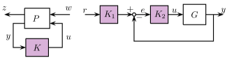
Figure 1. Black-box full-order controller $K$ on the left, structured 2-DOF control architecture with $K={\rm diag}(K_{1},K_{2})$ on the right.

More sophisticated controller structures $K(\mathbf{x})$ arise form architectures like for instance a 2-DOF control arrangement with feedback block $K_{2}$ and a set-point filter $K_{1}$ as in Fig. 1 (right). Suppose $K_{1}$ is the $1$st-order filter $K_{1}(s)=a/(s+a)$ and $K_{2}$ the PI feedback $K_{2}(s)=k_{P}+k_{I}/s$. Then the transfer $T_{ry}$ from $r$ to $y$ can be represented as the feedback connection of $P$ and $K(\mathbf{x},s)$ with

$$P:=\left[\begin{array}[]{c|ccc}A&0&0&B\\ \hline\cr C&0&0&D\\ 0&I&0&0\\ -C&0&I&-D\end{array}\right],$$

$$K(\mathbf{x},s):=\left[\begin{array}[]{cc}K_{1}(a,s)&0\\ 0&K_{2}(s,k_{P},k_{I})\\ \end{array}\right]\,,$$

and gathering tunable elements in $\mathbf{x}=(a,k_{P},k_{I})$.

In much the same way arbitrary multi-loop interconnections of fixed-model elements with tunable controller blocks $K_{i}(\mathbf{x})$ can be re-arranged as in Fig. 2, so that $K(\mathbf{x})$ captures all tunable blocks in a decentralized structure general enough to cover most engineering applications.

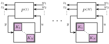
Figure 2. Synthesis of $K={\rm diag}(K_{1},\dots,K_{N})$ against multiple requirements or models $P^{(1)},\dots,P^{(M)}$. Each $K_{i}(\mathbf{x})$ can be structured.

The structure concept is equally useful to deal with the second central challenge in control design: system uncertainty. The latter may be handled with $\mu$-synthesis techniques [2] if a parametric uncertain model is available. A less ambitious but often more practical alternative consists in optimizing the structured controller $K(\mathbf{x})$ against a finite set of plants $P^{(1)},\dots,P^{(M)}$ representing model variations due to uncertainty, aging, sensor and actuator breakdown, un-modeled dynamics, in tandem with the robustness and performance specifications. This is again formally covered by Fig. 2 and leads to a multi-objective constrained optimization problem of the form

(22) $$\begin{array}[]{ll}\mbox{minimize}&f(\mathbf{x})=\max\limits_{k\in{\rm SOFT},i\in I_{k}}\|T_{w_{i}z_{i}}^{(k)}(K(\mathbf{x}))\|\\ \mbox{subject to}&g(\mathbf{x})=\max\limits_{k\in{\rm HARD},j\in J_{k}}\|T_{w_{j}z_{j}}^{(k)}(K(\mathbf{x}))\|\leq 1\\ &K(\mathbf{x})\mbox{ structured and stabilizing}\\ &\mathbf{x}\in\mathbb{R}^{n}\end{array}$$

where $T_{w_{i}z_{i}}^{(k)}$ denotes the $i$th closed-loop robustness or performance channel $w_{i}\to z_{i}$ for the $k$-th plant model $P^{(k)}$. SOFT and HARD denote index sets taken over a finite set of specifications, say in $\left\{1,\ldots,M\right\}$. The rationale of (22) is to minimize the worst-case cost of the soft constraints $\|T_{w_{i}z_{i}}^{(k)}\|$, $k\in\,$SOFT, while enforcing the hard constraints $\|T_{w_{j}z_{j}}^{(k)}\|\leq 1$, $k\in\,$HARD, which prevail over soft ones and are mandatory. In addition to local optimization (22), the problem can undergo a global optimization step in order to prove global stability and performance of the design, see [3, 4, 5].

2. Optimization Techniques Over the Years

During the late 1990s the necessity to develop design techniques for structured regulators $K(\mathbf{x})$ was recognized [6], and the limitations of synthesis methods based on algebraic Riccati equations or linear matrix inequalities (LMIs) became evident, as these techniques cannot provide structured controllers needed in practice. The lack of appropriate synthesis techniques for structured $K(\mathbf{x})$ led to the unfortunate situation, where sophisticated approaches like the $H_{\infty}$ paradigm developed by academia since the 1980s could not be brought to work for the design of those controller structures $K(\mathbf{x})$ preferred by practitioners. Design engineers had to continue to rely on heuristic and ad-hoc tuning techniques, with only limited scope and reliability. As an example: post-processing to reduce a black-box controller to a practical size is prone to failure. It may at best be considered a fill-in for a rigorous design method which directly computes a reduced-order controller. Similarly, hand-tuning of the parameters $\mathbf{x}$ remains a puzzling task because of the loop interactions, and fails as soon as complexity increases.

In the late 1990s and early 2000s, a change of methods was observed. Structured $H_{2}$- and $H_{\infty}$-synthesis problems (11) were addressed by bilinear matrix inequality (BMI) optimization, which used local optimization techniques based on the augmented Lagrangian method [6, 7, 8, 9], sequential semidefinite programming methods [10, 11], and non-smooth methods for BMIs [12, 13]. However, these techniques were based on the bounded real lemma or similar matrix inequalities, and were therefore of limited success due to the presence of Lyapunov variables, i.e. matrix-valued unknowns, whose dimension grows quadratically in $n_{P}+n_{K}$ and represents the bottleneck of that approach.

The epoch-making change occurs with the introduction of non-smooth optimization techniques [14, 15, 16, 17] to programs (11) and (22). Today non-smooth methods have superseded matrix inequality-based techniques and may be considered the state-of-art as far as realistic applications are concerned. The transition took almost a decade.

Alternative control-related local optimization techniques and heuristics include the gradient sampling technique of [18], and other derivative-free optimization as in [19, 20], particle swarm optimization, see [21] and references therein, and also evolutionary computation techniques [22]. All these classes do not exploit derivative information and rely on function evaluations only. They are therefore applicable to a broad variety of problems including those where function values arise from complex numerical simulations. The combinatorial nature of these techniques, however, limits their use to small problems with a few tens of variable. More significantly, these methods often lack a solid convergence theory. In contrast, as we have demonstrated over recent years, [15, 23, 24, 25] specialized non-smooth techniques are highly efficient in practice, are based on a sophisticated convergence theory, capable of solving medium size problems in a matter of seconds, and are still operational for large size problems with several hundreds of states.

3. Non-smooth optimization techniques

The benefit of the non-smooth casts (11) and (22) lies in the possibility to avoid searching for Lyapunov variables, a major advantage as their number $(n_{P}+n_{K})^{2}/2$ usually largely dominates $n$, the number of true decision parameters $\mathbf{x}$. Lyapunov variables do still occur implicitly in the function evaluation procedures, but this has no harmful effect for systems up to several hundred states. In abstract terms, a non-smooth optimization program has the form

(26) $$\begin{array}[]{ll}\mbox{minimize}&f(\mathbf{x})\\ \mbox{subject to}&g(\mathbf{x})\leq 0\\ &\mathbf{x}\in\mathbb{R}^{n}\end{array}$$

where $f,g:\mathbb{R}^{n}\to\mathbb{R}$ are locally Lipschitz functions and are easily identified from the cast in (22).

In the realm of convex optimization, non-smooth programs are conveniently addressed by so-called bundle methods, introduced in the late 1970s by Lemaréchal [26]. Bundle methods are used to solve difficult problems in integer programming or in stochastic optimization via Lagrangian relaxation. Extensions of the bundling technique to non-convex problems like (11) or (22) were first developed in [15, 16, 17, 27, 12], and in more abstract form, in [23]. Recently, we also extended bundle techniques to the trust-region framework [24, 25, 28], which leads to the first extension of the classical trust-region method to non-differential optimization supported by a valid convergence theory.

Fig. 3 shows a schematic view of a non-convex bundle method consisting of a descent-step generating inner loop (yellow block) comparable to a line search in smooth optimization, embedded into the outer loop (blue box), where serious iterates are processed, stopping criteria are applied, and the acceptance rules of traditional trust region techniques is assured. At the core of the interaction between inner and outer loop is the management of the proximity control parameter $\tau$, which governs the stepsize $\|\mathbf{x}-\mathbf{y}^{k}\|$ between trial steps $\mathbf{y}^{k}$ at the current serious iterate $\mathbf{x}$. Similar to the management of a trust region radius or of the stepsize in a linesearch, proximity control allows to force shorter trial steps if agreement of the local model with the true objective function is poor, and allows larger steps if agreement is satisfactory.

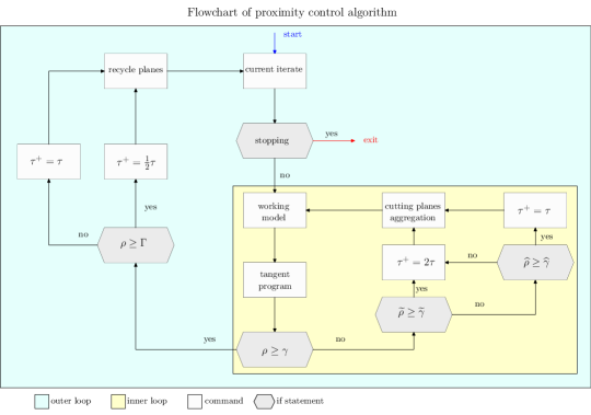
Figure 3. Flow chart of proximity control bundle algorithm

Oracle-based bundle methods traditionally assure global convergence in the sense of subsequences under the sole hypothesis that for every trial point $\mathbf{x}$ the function value $f(\mathbf{x})$ and one Clarke subgradient $\phi\in\partial f(\mathbf{x})$ are provided. In automatic control applications it is as a rule possible to provide more specific information, which may be exploited to speed up convergence [15].

Computing function value and gradients of the $H_{2}$-norm $f(\mathbf{x})=\|T_{wz}\left(P,K(\mathbf{x})\right)\|_{2}$ requires essentially the solution of two Lyapunov equations of size $n_{P}+n_{K}$, see [29]. For the $H_{\infty}$-norm, $f(\mathbf{x})=\|T_{wz}\left(P,K(\mathbf{x})\right)\|_{\infty}$, function evaluation is based on the Hamiltonian algorithm of [30, 31]. The Hamiltonian matrix is of size $n_{P}+n_{K}$, so that function evaluations may be costly for very large plant state dimension ($n_{P}>500$), even though the number of outer loop iterations of the bundle algorithm is not affected by a large $n_{P}$ and generally relates to $n$, the dimension of $\mathbf{x}$. The additional cost for subgradient computation for large $n_{P}$ is relatively cheap as it relies on linear algebra [15]. Function and subgradient evaluations for $H_{\infty}$ and $H_{2}$ norms are typically obtained in $\mathcal{O}\left((n_{P}+n_{K})^{3}\right)$ flops.

4. Computational Tools

Our non-smooth optimization methods became available to the engineering community since 2010 via the MATLAB Robust Control Toolbox [32, 33]. Routines hinfstruct, looptune  and systune  are versatile enough to define and combine tunable blocks $K_{i}(\mathbf{x})$, to build and aggregate multiple models and design requirements on $T_{wz}^{(k)}$ of different nature, and to provide suitable validation tools. Their implementation was carried out in cooperation with P. Gahinet (MathWorks). These routines further exploit the structure of problem (22) to enhance efficiency, see [16] and [15].

It should be mentioned that design problems with multiple hard constraints are inherently complex and generally NP-hard, so that exhaustive methods fail even for small to medium size problems. The principled decision made in [15], and reflected in the MATLAB tools, is to rely on local optimization techniques instead. This leads to weaker convergence certificates, but has the advantage to work successfully in practice. In the same vein, in (22) it is preferable to rely on a mixture of soft and hard requirements, for instance, by the use of exact penalty functions [14]. Key features implemented in the mentioned MATLAB routines are discussed in [34, 33, 16].

5. Applications

Design of a feedback regulator is an interactive process, in which tools like systune, looptune   or hinfstruct   support the designer in various ways. In this section we illustrate their enormous potential by showing that even infinite-dimensional systems may be successfully addressed by these tools. For a plethora of design examples for real-rational systems including parametric and complex dynamic uncertainty we refer to [3, 24, 4, 28, 25]. For recent applications of our tools in real-world applications see also [35], where it is in particular explained how hinfstruct helped in 2014 to save the Rosetta mission. Another important application of hinfstruct is the design of the atmospheric flight pilot for the ARIANE VI launcher by the Ariane Group [36].

5.1. Illustrative example

We discuss boundary control of a wave equation with anti-stable damping,

$$x_{tt}(\xi,t) =x_{\xi\xi}(\xi,t),\;\;t\geq 0,\xi\in[0,1]$$

(27) $$x_{\xi}(0,t) =-qx_{t}(0,t),\;\;q>0,q\not=1$$

$$x_{\xi}(1,t) =u(t).$$

where notations $x_{t}$, $x_{\xi}$ are partial derivatives of $x$ with respect to time and space, respectively. In (5.1), $x(\cdot,t),x_{t}(\cdot,t)$ is the state, the control applied at the boundary $\xi=1$ is $u(t)$, and we assume that the measured outputs are

(28) $$y_{1}(t)=x(0,t),y_{2}(t)=x(1,t),y_{3}(t)=x_{t}(1,t).$$

The system has been discussed previously in [37, 38, 39] and has been proposed for the control of slip-strick vibrations in drilling devices [40]. Here measurements $y_{1},y_{2}$ correspond to the angular positions of the drill string at the top and bottom level, $y_{3}$ measures angular speed at the top level, while control corresponds to a reference velocity at the top. The friction characteristics at the bottom level are characterized by the parameter $q$, and the control objective is to maintain a constant angular velocity at the bottom.

Similar models have been used to control pressure fields in duct combustion dynamics, see [41]. The challenge in (5.1), (28) is to design implementable controllers despite the use of an infinite-dimensional system model.

The transfer function of (5.1) is obtained from:

$$G(\xi,s)=\frac{x(\xi,s)}{u(s)}=\frac{1}{s}\cdot\frac{(1-q)e^{s\xi}+(1+q)e^{-s\xi}}{(1-q)e^{s}-(1+q)e^{-s}},$$

which in view of (28) leads to $G(s)=[G_{1};G_{2};G_{3}]=[G(0,s);G(1,s);sG(1,s)]$.

Putting $G$ in feedback with the controller $K_{0}=[0\;0\;1]$ leads to $\widehat{G}=G/(1+G_{3})$, where

(29) $$\widehat{G}(s)=\begin{bmatrix}\frac{1}{s(1-q)}\vspace{.2cm}\\ \frac{1+Q}{2s}\vspace{.2cm}\\ \frac{1}{2}\end{bmatrix}+\begin{bmatrix}-\frac{1-e^{-s}}{s(1-q)}\vspace{.2cm}\\ -\frac{Q(1-e^{-2s})}{2s}\\ \vspace{.2cm}\frac{Q}{2}e^{-2s}\end{bmatrix}=:\widetilde{G}(s)+\Phi(s).$$

Here $\widetilde{G}$ is real-rational and unstable, while $\Phi$ is stable but infinite dimensional. Now we use the fact that stability of the closed loop $(\widetilde{G}+\Phi,K)$ is equivalent to stability of the loop $(\widetilde{G},{\tt feedback}(K,\Phi))$ upon defining ${\tt feedback}(M,N):=M(I+NM)^{-1}\,.$ The loop transformation is explained in Fig. 4, see also [42].

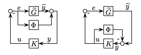
Figure 4. Stability of the closed-loop $(\widetilde{G}+\Phi,K)$ is equivalent to stability of the closed-loop $(\widetilde{G},{\tt feedback}(K,\Phi))$.

Using (29) we construct a finite-dimensional structured controller $\widetilde{K}=\widetilde{K}(\mathbf{x})$ which stabilizes $\widetilde{G}$. The controller $K$ stabilizing $\widehat{G}$ in (29) is then recovered from $\widetilde{K}$ through the equation $\widetilde{K}={\tt feedback}(K,\Phi)$, which when inverted gives $K={\tt feedback}(\widetilde{K},-\Phi)$. The overall controller for (5.1) is $K^{*}=K_{0}+K$, and since along with $K$ only delays appear in $\Phi$, the controller $K^{*}$ is implementable.

Construction of $\widetilde{K}$ uses systune  with pole placement via TuningGoal.Poles, imposing that closed-loop poles have a minimum decay of 0.9, minimum damping of 0.9, and a maximum frequency of 4.0. The controller structure is chosen as static, so that $\mathbf{x}\in\mathbb{R}^{3}$. A simulation with $K^{*}$ is shown in Fig. 5 (bottom) and some acceleration over the backstepping controller from [39] (top) is observed.

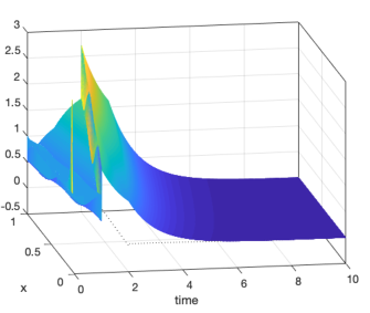
Figure 5. Wave equation. Simulations for $K$ obtained by backstepping control (top) [39] and $K^{*}=K_{0}+K$ obtained by optimizing ${\tt feedback}(\widetilde{G},\widetilde{K})$ via systune  (bottom). Both controllers are $\infty$-dimensional, but implementable.

5.2. Gain-scheduling control

Our last study is when the parameter $q\geq 0$ is uncertain or allowed to vary in time with sufficiently slow variations as in [43]. We assume that a nominal $q_{0}>0$ and an uncertain interval $[\underline{q},\overline{q}]$ with $q_{0}\in(\underline{q},\overline{q})$ and $1\not\in[\underline{q},\overline{q}]$ are given.

The following scheduling scenarios, all leading to implementable controllers, are possible. (a) Computing a nominal controller $\widetilde{K}$ at $q_{0}$ as before, and scheduling through $\Phi(q)$, which depends explicitly on $q$, so that $K^{(1)}(q)=K_{0}+{\tt feedback}(\widetilde{K},-\Phi(q))$. (b) Computing $\widetilde{K}(q)$ which depends on $q$, and using $K^{(2)}(q)=K_{0}+{\tt feedback}(\widetilde{K}(q),-\Phi(q))$.

While (a) uses (11) based on [15, 17] and available in systune, we show that one can also apply (11) to case (b). We use Fig. 4 to work in the finite-dimensional system $(\widetilde{G}(q),\widetilde{K}(q))$, where plant and controller now depend on $q$, which is a parameter-varying design.

For that we have to decide on a parametric form of the controller $\widetilde{K}(q)$, which we choose as

$$\widetilde{K}(q,\mathbf{x})=\widetilde{K}(q_{0})+(q-q_{0})\widetilde{K}_{1}(\mathbf{x})+(q-q_{0})^{2}\widetilde{K}_{2}(\mathbf{x}),$$

and where we adopted the simple static form $\widetilde{K}_{1}(\mathbf{x})=[\mathbf{x}_{1}\;\mathbf{x}_{2}\;\mathbf{x}_{3}],\widetilde{K}_{2}=[\mathbf{x}_{4}\;\mathbf{x}_{5}\;\mathbf{x}_{6}]$, featuring a total of 6 tunable parameters. The nominal $\widetilde{K}(q_{0})$ is obtained via (11) as above. For $q_{0}=3$ this leads to $\widetilde{K}(q_{0})=[-1.049\;-1.049\;-0.05402]$, computed via systune.

With the parametric form $\widetilde{K}(q,\mathbf{x})$ fixed, we now use again the feedback system $(\widetilde{G}(q),\widetilde{K}(q))$ in Fig. 4 and design a parametric robust controller using the method of [4], which is included in the systune  package and used by default if an uncertain closed-loop is entered. The tuning goals are chosen as constraints on closed-loop poles including minimum decay of 0.7, minimum damping of 0.9, with maximum frequency $2$. The controller obtained is (with $q_{0}=3$)

$$\widetilde{K}(q,\mathbf{x}^{*})=\widetilde{K}(q_{0})+(q-q_{0})\widetilde{K}_{1}(\mathbf{x}^{*})+(q-q_{0})^{2}\widetilde{K}_{2}(\mathbf{x}^{*}),$$

with $\widetilde{K}_{1}=[-0.1102,-0.1102,-0.1053]$, $\widetilde{K}_{2}=[0.03901,0.03901,0.02855]$, and we retrieve the final parameter varying controller for $G(q)$ as

$$K^{(2)}(q)=K_{0}+{\tt feedback}(\widetilde{K}(q,\mathbf{x}^{*}),-\Phi(q)).$$

Nominal and scheduled controllers are compared in simulation in Figs. 6, 7, and 8, which indicate that $K^{(2)}(q)$ achieves the best performance for frozen-in-time values $q\in[2,4]$. All controllers are easily implementable, since only real-rational elements in combination with delays are used.

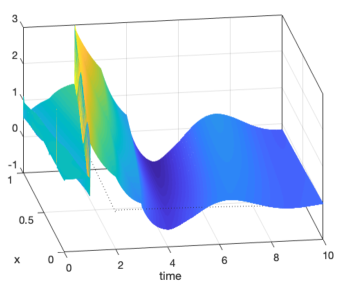
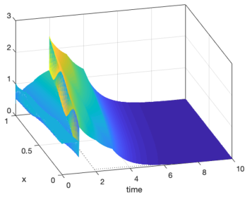
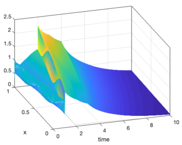
Figure 6. Synthesis at nominal $q_{0}=3$. Simulations of nominal $K=K_{0}+{\tt feedback}(\widetilde{K},\Phi(3))$ for $q=2,3,4$. Nominal controller is robustly stable over $[\underline{q},\overline{q}]$.

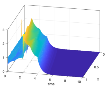
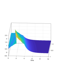
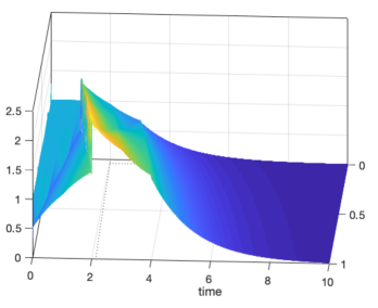
Figure 7. Method 1. $\widetilde{K}$ obtained for nominal $q=3$, but scheduled $K(q)=K_{0}+{\tt feedback}(\widetilde{K},\Phi(q))$. Simulations for $q=2$ top, $q=3$ middle, $q=4$ bottom

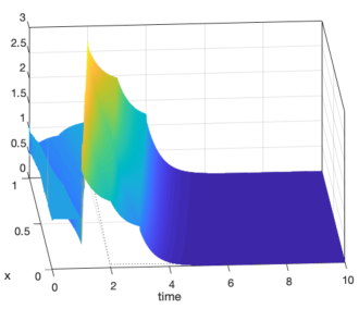
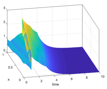
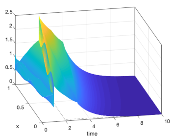
Figure 8. Method 2. $\widetilde{K}(q)=\widetilde{K}_{\rm nom}+(q-3)\widetilde{K}_{1}+(q-3)^{2}\widetilde{K}_{2}$ and $K(q)=K_{0}+{\tt feedback}(\widetilde{K}(q),\Phi(q)$. Simulations for $q=2,3,4$

The non-smooth program (26) was solved with systune  in $30$s CPU on a Mac OS X with $2.66$ GHz Intel Core i7 and $8$ GB RAM. The reader is referred to the MATLAB Control Toolbox 2018b and higher versions for additional examples. More details on this study can be found in [44].

References

- [1] K. Zhou, J. C. Doyle, K. Glover, Robust and Optimal Control, Prentice Hall, 1996.
- [2] G. Stein, J. Doyle, Beyond singular values and loopshapes, AIAA Journal of Guidance and Control 14 (1991) 5–16.
- [3] L. Ravanbod, D. Noll, P. Apkarian, Branch and bound algorithm with applications to robust stability, Journal of Global Optimization 67 (3) (2017) 553–579.
- [4] P. Apkarian, M. N. Dao, D. Noll, Parametric robust structured control design, IEEE Transactions on Automatic Control 60 (7) (2015) 1857–1869.
- [5] P. Apkarian, D. Noll, L. Ravanbod, Computing the structured distance to instability, in: SIAM Conference on Control and its Applications, 2015, pp. 423–430. http://dx.doi.org/10.1137/1.9781611974072.58 doi:10.1137/1.9781611974072.58.
- [6] B. Fares, P. Apkarian, D. Noll, An augmented Lagrangian method for a class of LMI-constrained problems in robust control theory, Int. J. Control 74 (4) (2001) 348–360.
- [7] D. Noll, M. Torki, P. Apkarian, Partially augmented Lagrangian method for matrix inequality constraints, SIAM Journal on Optimization 15 (1) (2004) 161–184.
- [8] M. Kocvara, M. Stingl, A code for convex nonlinear and semidefinite programming, Optimization Methods and Software 18 (3) (2003) 317–333.
- [9] D. Noll, Local convergence of an augmented Lagrangian method for matrix inequality constrained programming, Optimization Methods and Software 22 (5) (2007) 777–802.
- [10] B. Fares, D. Noll, P. Apkarian, Robust control via sequential semidefinite programming, SIAM J. on Control and Optimization 40 (6) (2002) 1791–1820.
- [11] P. Apkarian, D. Noll, J. B. Thevenet, H. D. Tuan, A spectral quadratic-SDP method with applications to fixed-order and synthesis, European J. of Control 10 (6) (2003) 527–538.
- [12] D. Noll, O. Prot, P. Apkarian, A proximity control algorithm to minimize nonsmooth and nonconvex semi-infinite maximum eigenvalue functions, Jounal of Convex Analysis 16 (3 & 4) (2009) 641–666.
- [13] C. Lemaréchal, F. Oustry, Nonsmooth algorithms to solve semidefinite programs, SIAM Advances in Linear Matrix Inequality Methods in Control series, ed. L. El Ghaoui & S.-I. Niculescu.
- [14] D. Noll, P. Apkarian, Spectral bundle methods for nonconvex maximum eigenvalue functions: first-order methods, Mathematical Programming Series B 104 (2) (2005) 701–727.
- [15] P. Apkarian, D. Noll, Nonsmooth synthesis, IEEE Trans. Aut. Control 51 (1) (2006) 71–86.
- [16] P. Apkarian, D. Noll, Nonsmooth optimization for multiband frequency domain control design, Automatica 43 (4) (2007) 724–731.
- [17] P. Apkarian, D. Noll, Nonsmooth optimization for multidisk synthesis, European J. of Control 12 (3) (2006) 229–244.
- [18] J. Burke, A. Lewis, M. Overton, A robust gradient sampling algorithm for nonsmooth, nonconvex optimization, SIAM Journal on Optimization 15 (2005) 751–779.
- [19] T. G. Kolda, R. M. Lewis, V. Torczon, Optimization by direct search: new perspectives on some classical and modern methods, SIAM Review 45 (3) (2003) 385–482.
- [20] P. Apkarian, D. Noll, Controller design via nonsmooth multi-directional search, SIAM Journal on Control and Optimization 44 (6) (2006) 1923–1949.
- [21] A. Oi, C. Nakazawa, T. Matsui, H. Fujiwara, K. Matsumoto, H. Nishida, J. Ando, M. Kawaura, Development of PSO-based PID tuning method, in: International Conference on Control, Automation and Systems, 2008, pp. 1917 –1920.
- [22] J. Lieslehto, PID controller tuning using evolutionary programming, in: American Control Conference, Vol. 4, 2001, pp. 2828 –2833.
- [23] D. Noll, O. Prot, A. Rondepierre, A proximity control algorithm to minimize nonsmooth and nonconvex functions, Pacific J. of Optimization 4 (3) (2008) 571–604.
- [24] P. Apkarian, D. Noll, L. Ravanbod, Nonsmooth bundle trust-region algorithm with applications to robust stability, Set-Valued and Variational Analysis 24 (1) (2016) 115–148.
- [25] P. Apkarian, D. Noll, L. Ravanbod, Non-smooth optimization for robust control of infinite-dimensional systems, Set-Valued and Variational Analysis 26 (2) (2018) 405–429.
- [26] C. Lemaréchal, An extension of Davidson’s methods to nondifferentiable problems, in: M. L. Balinski, P. Wolfe (Eds.), Math. Programming Study 3, Nondifferentiable Optimization, North-Holland, 1975, pp. 95–109.
- [27] P. Apkarian, D. Noll, O. Prot, A trust region spectral bundle method for nonconvex eigenvalue optimization, SIAM J. on Optimization 19 (1) (2008) 281–306.
- [28] P. Apkarian, D. Noll, Structured -control of infinite dimensional systems, Int. J. Robust Nonlin. Control 28 (9) (2018) 3212–3238.
- [29] P. Apkarian, D. Noll, A. Rondepierre, Mixed control via nonsmooth optimization, in: Proc. of the 46th IEEE Conference on Decision and Control, New Orleans, LA, 2007, pp. 4110–4115.
- [30] P. Benner, V. Sima, M. Voigt, -norm computation for continuous-time descriptor systems using structured matrix pencils, IEEE Trans. Aut. Control 57 (1) (2012) 233–238.
- [31] S. Boyd, V. Balakrishnan, P. Kabamba, A bisection method for computing the norm of a transfer matrix and related problems, Mathematics of Control, Signals, and Systems 2 (3) (1989) 207–219.
- [32] Robust Control Toolbox 4.2, The MathWorks Inc. Natick, MA, USA.
- [33] P. Gahinet, P. Apkarian, Structured synthesis in MATLAB, in: Proc. IFAC World Congress, Milan, Italy, 2011, pp. 1435–1440.
- [34] P. Apkarian, Tuning controllers against multiple design requirements, in: American Control Conference (ACC), 2013, 2013, pp. 3888–3893.
- [35] A. Falcoz, C. Pittet, S. Bennani, A. Guignard, C. Bayart, B. Frapard, Systematic design methods of robust and structured controllers for satellites. Application to the refinement of Rosetta’s orbit controller, CEAS Space Journal 7 (2015) 319–334. http://dx.doi.org/10.1007/s12567-015-0099-8 doi:10.1007/s12567-015-0099-8.
- [36] M. Ganet-Schoeller, J. Desmariaux, C. Combier, Structured control for future european launchers, AeroSpaceLab 13 (2017) 2–10.
- [37] A. Smyshlyaev, M. Krstic, Boundary control of an anti-stable wave equation with anti-damping on the uncontrolled boundary, Systems and Control Letters 58 (2009) 617–623.
- [38] E. Fridman, Introduction to Time-Delay Systems, Systems and Control, Foundations and Applications, Birkhäuser Basel, 2014.
- [39] D. Bresch-Pietri, M. Krstic, Output-feedback adaptive control of a wave PDE with boundary anti-damping, Automatica 50 (5) (2014) 1407–1415.
- [40] M. Saldivar, S. Mondié, J.-J. Loiseau, V. Rasvan, Stick-slip oscillations in oilwell drillings: distributed parameter and neutral type retarded model approaches (2011).
- [41] M. DeQueiroz, C. D. Rahn, Boundary control of vibrations and noise in distributed parameter systems: an overview, Mechanical Systems and Signal Processing 16 (1) (2002) 19–38.
- [42] A. A. Moelja, G. Meinsma, Parametrization of stabilizing controllers for systems with multiple i/o delays, IFAC Proceedings Volumes 36 (19) (2003) 351 – 356, 4th IFAC Workshop on Time Delay Systems (TDS 2003), Rocquencourt, France, 8-10 September 2003.
- [43] J. F. Shamma, M. Athans, Analysis of Gain Scheduled Control for Nonlinear Plants, IEEE Trans. Aut. Control 35 (8) (1990) 898–907.
- [44] P. Apkarian, D. Noll, Boundary control of partial differential equations using frequency domain optimization techniques arXiv:1905.06786v1 (2019) pages 1–22.