Abstract

The literature suggests that autonomous vehicles (AVs) may drastically change the user experience of private automobile travel by allowing users to engage in productive or relaxing activities while travelling. As a consequence, the generalised cost of car travel may decrease, and car users may become less sensitive to travel time. By facilitating private motorised mobility, AVs may eventually impact land use and households’ residential location choices. This paper seeks to advance the understanding of the potential impacts of AVs on travel behaviour and land use by investigating stated preferences for combinations of residential locations and travel options for the commute in the context of autonomous automobile travel. Our analysis draws from a stated preference survey, which was completed by 512 commuters from the Sydney metropolitan area in Australia and provides insights into travel time valuations in a long-term decision-making context. For the analysis of the stated choice data, mixed logit models are estimated. Based on the empirical results, no changes in the valuation of travel time due to the advent of AVs should be expected. However, given the hypothetical nature of the stated preference survey, the results may be affected by methodological limitations.

Keywords: connected and autonomous vehicles, residential location choice, value of time, stated choice, mixed logit

1 Introduction

In light of recent technological advancements in the fields of vehicle automation and connection, connected and autonomous vehicles (AVs) with advanced self-driving capabilities are anticipated to be available to the consumer mass market in the not-so-distant future (e.g. Burns, , 2013; Fagnant and Kockelman, , 2015; Nieuwenhuijsen et al., , 2018; Wadud et al., , 2016). In their technologically most advanced stage, AVs are expected to be fully automated and to operate autonomously, not requiring any control input by the user (National Highway Traffic Safety Administration, , 2013; Society of Automotive Engineers International, , 2016). AVs may catalyse a profound transformation of the transport sector by making private motorised mobility safer (e.g. Anderson et al., , 2014; Fagnant and Kockelman, , 2015; Sparrow and Howard, , 2017), more affordable (e.g. Bösch et al., , 2018; Burns et al., , 2013) and more accessible to user groups that are currently unwilling or unable to drive (e.g. Anderson et al., , 2014; Fagnant and Kockelman, , 2015; Harper et al., , 2016). Moreover, AVs with full self-driving capabilities may substantially alter the user experience of private motorised mobility by allowing users to engage in productive or relaxing activities while travelling in an AV (e.g. Le Vine et al., , 2015; Pudāne et al., 2018a, ). In turn, some travellers’ generalised cost of car travel may decrease, and a proportion of travellers may become less sensitive to travel time. As AVs facilitate private motorised mobility, the accessibility of locations may increase and eventually, AVs may fuel urban sprawl and suburbanisation by affecting the location choices of households and firms (Meyer et al., , 2017; Milakis et al., , 2018).

Strategic policy processes in the domain of integrated transport and land use planning depend on future-proof estimates of population sensitivities with respect to travel- and lifestyle-related variables (e.g. Bhat and Guo, , 2007; Pinjari et al., , 2007; Schwanen and Mokhtarian, , 2005). The lifestyle-based approach to travel behaviour analysis recognises complex interdependencies between travel behaviour, residential location and lifestyle orientations (Van Acker et al., , 2010): It is understood that travel behaviour (e.g. mode choice) and residential location are co-determined by lifestyle goals pertaining to travel, neighbourhood and housing (Bhat and Guo, , 2007; Pinjari et al., , 2007; Schwanen and Mokhtarian, , 2005). As a consequence, a household’s housing search process involves trade-offs between a variety of travel- and lifestyle-related variables (Guo et al., , 2018; Rouwendal and Meijer, , 2001; Walker and Li, , 2006); in particular, the spatial search process requires households to balance housing expenses against household members’ travel times and costs to reach frequently-visited destinations such as the workplace (So et al., , 2001). With the advent of AVs, some travellers’ generalised cost of car travel may decrease. From this supposition, the question arises as to what extent the advent of AVs may affect preferences for travel and residential location.

The current paper seeks to advance the understanding of the potential impacts of autonomous driving on travel behaviour and land use by investigating preferences for residential locations and travel options for the commute in the context of autonomous driving. To this end, we designed and implemented a stated preference survey, which was completed by 512 commuters from the Sydney metropolitan area in Australia. The survey featured a discrete choice experiment requiring respondents to jointly choose a housing option and a travel option for the commute, whereby the presented travel options included the transport modes conventional car, self-driving car and public transit. In multiple scenarios, attributes such as housing and commute costs as well as commute travel times were manipulated. For the analysis of the stated choice data, a mixed multinomial logit model accommodating unobserved taste variation and flexible substitution patterns is estimated. The estimation results provide insights into travel time valuations for autonomous driving in a long-term decision-making context.

We organise the remainder of this paper as follows: First, we present a review of pertinent literature. Then, we describe the survey design and the data collection and explain the modelling approach. Next, we present the results. We conclude with a general discussion of the findings.

2 Literature review

A rapidly-expanding body of literature is concerned with evaluating the economic, societal and environmental implications of autonomous driving (for a comprehensive review, see Milakis et al., , 2017). Within this body of literature, several studies explicitly investigate the impacts of autonomous driving on travel behaviour and land use. Soteropoulos et al., (2018) present a systematic review of 37 studies on the topic. The majority of these studies rely on activity-based or agent-based modelling approaches and find that the advent of AVs may lead to increases in vehicle kilometres travelled, lower levels of public transit and active mode use as well as to suburbanisation and urban sprawl. Soteropoulos et al., (2018) observe that the findings of the considered studies may be sensitive to the underlying modelling assumptions, particularly in regards to the value of time for autonomous driving and the business models under which AVs become available.

Of the studies reviewed by Soteropoulos et al., (2018), we highlight three studies that focus on residential location choices. Using a spatial general equilibrium model, Gelauff et al., (2017) analyse changes in home and job location as well as in commute mode choice in the context of two automation scenarios in the Netherlands. In the first scenario, AVs permit productive time use during long-distance car travel; in the second scenario, AVs enable efficient door-to-door transport. The authors find that the first scenario results in urban sprawl, while the second scenario results in population concentration in core area. Employing a strategic land use transport interaction model, Thakur et al., (2016) investigate changes in residential location choices and travel behaviour in response to the availability of AVs in the Melbourne metropolitan area in Australia. Assuming that the value of time for travel by AV is 50% of the value of time for travel by conventional car, the authors forecast a population reduction of 4% in central areas and a population increase of 3% in outer suburbs. Zhang and Guhathakurta, (2018) predict residential location choices in the Atlanta metropolitan area in the USA in the presence of shared autonomous vehicles (SAVs, e.g. Fagnant and Kockelman, , 2014; Krueger et al., , 2016). The study relies on an agent-based simulation model, which couples a residential location choice model assuming extant residential location preferences and a SAV simulation model assuming that the value of time for travel by SAV is between 0% and 75% of the current value of time for travel by conventional car. The authors find that the presence of SAVs may result in an increase in commute vehicle kilometres travelled across all considered market segments.

Analysing data sourced from a survey among 347 individuals from the city of Austin in the USA, Bansal et al., (2016) develop an ordered probit model to explain whether respondents would shift their home locations, if AVs and SAVs became available. The authors find that respondents who live in dense residential neighbourhoods, who have a greater number of children and who have obtained a Bachelor’s degree are comparatively more likely to indicate that they would consider to live further away from central areas; by contrast, respondents who are familiar with car sharing and who carry a smartphone are comparatively more likely to indicate that they would consider to move closer to central areas, if AVs and SAVs became available. Relatedly, Bansal and Kockelman, (2018) draw from a questionnaire-based survey in Texas, USA and find that 81.5% of 1,088 respondents would not consider to change their home location, once AVs become available. Moreover, Milakis et al., (2018) apply the Q-method to analyse expert opinions on the possible accessibility impacts of autonomous driving. The authors extract three main viewpoints from 17 expert responses: First, initial accessibility gains may be neutralised by increased travel demand; second, autonomous driving will lead to increased density in the urban core and to decreased density in surrounding areas; third; the accessibility benefits will be unequally distributed and will only be enjoyed by those who can afford autonomous driving.

A second growing body of literature investigates preferences for different aspects of autonomous driving with the help of discrete choice experiments (see Gkartzonikas and Gkritza, , 2019, for a comprehensive review). The studies within this body of literature consider short- and long-term decision contexts, but interdependencies between preferences for residential location and travel behaviour have not been explicitly investigated. Daziano et al., (2017) analyse stated preferences of households in the USA for different levels of private vehicle automation. Relatedly, (Shabanpour et al., , 2018) investigate stated preferences of individuals living in the Chicago metropolitan area in the USA for attributes and ownership of AVs. Moreover, Haboucha et al., (2017) examine stated preferences of commuters in Israel and the USA for owning and sharing AVs. Krueger et al., (2016) and Winter et al., (2017) examine stated preferences for the use of SAVs in Australia and respectively the Netherlands. Similarly, Kolarova et al., (2017) investigate stated preferences for the use of SAVs and privately-owned AVs in Germany.

Preferences for combinations of housing and travel options for the commute have been studied in a general context without consideration of autonomous driving. For example, Rouwendal and Meijer, (2001) analyse Dutch workers’ stated preferences for combinations of housing, employment and commuting, using conditional and mixed multinomial logit models. The authors find that workers are generally averse to commuting but may accept longer commutes in exchange for some housing attributes. In particular, dual-earner households are found to show a preference for living in small- and medium-sized cities. Walker and Li, (2006) estimate a latent class multinomial logit model to analyse stated lifestyle and travel preferences of residents of Portland, Oregon, USA. The authors discern three lifestyle segments, namely suburban dwellers who prefer auto-oriented lifestyles with larger residences in suburban neighbourhoods that offer services and amenities nearby, transit riders who prefer to public-transportation-oriented lifestyles in suburban neighbourhoods, and urban dwellers who prefer auto-oriented lifestyles in smaller homes in urban neighbourhoods. Using stated choice data collected in Shenyang, China, Guo et al., (2018) develop a mixed multinomial logit model with error components to jointly analyse preferences for home relocation, job change and commute mode choice. The authors find substantial unobserved heterogeneity in tastes and substitution patterns.

To conclude, a review of the pertinent literature reveals that the potential impacts of autonomous driving on trade-offs between key travel- and lifestyle-related variables have not been sufficiently quantified. The current paper seeks to advance the literature in this regard by investigating stated preferences for combinations of residential location options and different commute travel options in the context of autonomous driving.

3 Methodology

3.1 Survey design and data collection

Data for this research study were collected via a web-based stated preference survey, which was completed by 512 residents of the Sydney metropolitan area in Australia. The survey comprised two parts: The first part requested information about respondents’ socio-demographic characteristics and their current commuting and housing arrangements; the second part featured a stated choice experiment requiring respondents to jointly choose a housing option and a travel option for the commute.

3.1.1 Choice tasks and alternatives

The stated choice experiment consisted of eight choice tasks, which required respondents to jointly choose one of two housing options and a travel option for the commute. The travel options were labelled “conventional car”, “self-driving car” and “public transportation”; if a respondent indicated that she did not hold a valid driving license, the option labelled “conventional car” was not displayed. The choice tasks were presented in a conjoint format (see Figure 1).

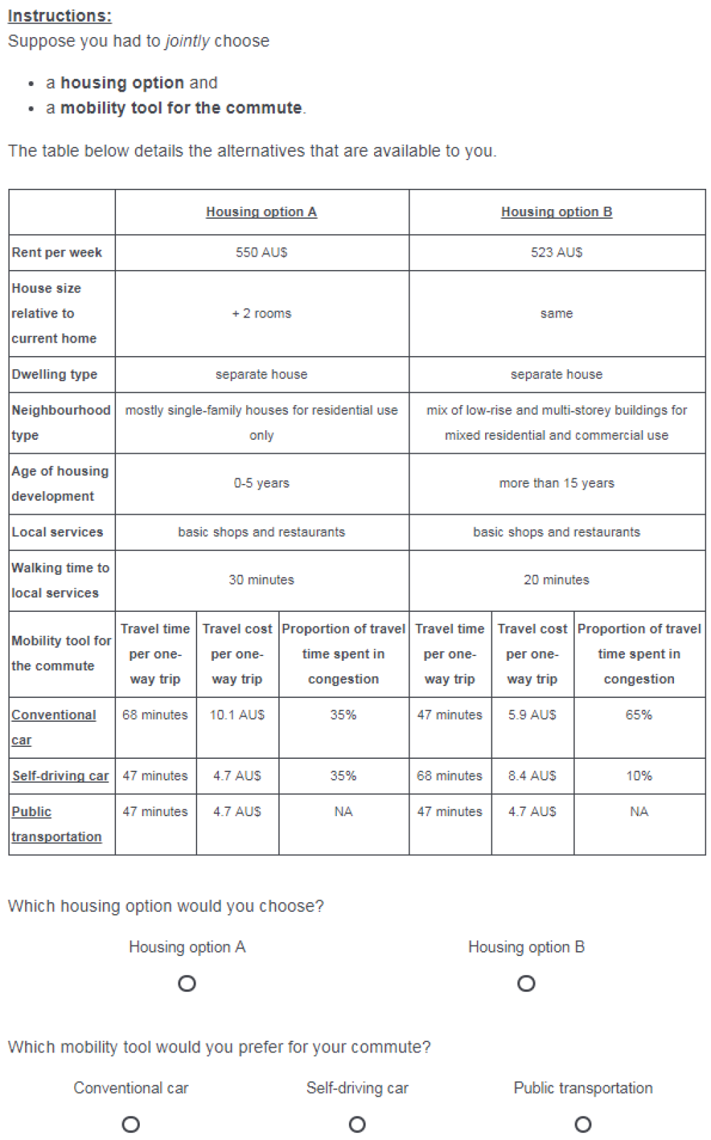
Figure 1: Example of a stated choice task

3.1.2 Attributes

The housing options were characterised by seven attributes, namely the weekly housing cost, the house size relative to the respondent’s current home, the dwelling type, the age of the housing development, the neighbourhood type, the presence of local services and the walking time to local services. If a respondent indicated to be a renter, the attribute was labelled “rent per week”. If a respondent indicated to live in a mortgaged home, the attribute was labelled “mortgage payment per week”. The selection of the housing attributes was inspired by other stated choice experiments that have appeared in the literature (Dubernet and Axhausen, , 2016; Rouwendal and Meijer, , 2001; Walker and Li, , 2006). The travel options for the commute were characterised by three attributes, namely the travel time per one-way trip, the travel cost per one-way trip and the proportion of travel time usually spent in congestion. Each of the housing options entailed different attribute values for the commute travel options such that the two choice dimensions depended on one another. To personalise the choice tasks, the attributes housing cost and travel time were pivoted around the respondent’s status quo. Table 1 gives a summary of the attributes and their levels. The experimental design of the choice tasks is based on orthogonal main-effect arrays and was created with the support.CE package for R (Aizaki, , 2012).

Attribute	Description and levels
Housing
Housing cost	• Three levels, pivoted around status quo – reference = $\min\{$ 6,500 AUD, $\max\{$150 AUD, current weekly housing cost in AUD$\}\}$ – pivot factors = $\{$0.95, 1.00, 1.05$\}$
Additional number of rooms	• Three levels, not pivoted – levels = $\{$0, 1, 2$\}$
Dwelling type	• Three levels, not pivoted – levels = $\{$unit, townhouse, separate house$\}$
Neighbourhood type	• Three levels, not pivoted – levels = $\{$unit, townhouse, separate house$\}$
Local services	• Three levels, not pivoted – levels = $\{$no shops, basic shops and restaurants, basic plus specialty shops and restaurants$\}$
Walking time to local services, if local services are available	• Three levels, not pivoted – levels = $\{$10 minutes, 20 minutes, 30 minutes$\}$
Mobility tools
Travel time	• Three levels, pivoted around status quo – reference = $\min\{$80 minutes, $\max\{$30 minutes, current commute time per one-way-trip in minutes$\}\}$ – pivot factors = $\{$1.05, 1.25, 1.5$\}$
Travel cost	• Three levels, pivoted – reference = hypothetical travel time of the mode – pivot factors = $\{$0.100 $\frac{\mbox{AUD}}{\mbox{minutes}}$, 0.125 $\frac{\mbox{AUD}}{\mbox{minutes}}$, 0.150 $\frac{\mbox{AUD}}{\mbox{minutes}}$$\}$
Proportion of travel time spent in congestion	• Three levels, not pivoted – levels = $\{$10%, 35%, 65%$\}$

Table 1: Attributes and attribute levels

3.1.3 Instructions

Prior to the presentation of the choice tasks, respondents were shown detailed instructions about the stated choice experiment. Respondents were told that they had to jointly choose a housing option and a preferred travel option for the commute. Moreover, the nature of the the travel options was explained to the respondents. Images were used to illustrate the experience of using one of the travel options. The travel option “self-driving car” was defined in accordance with SAE level 5 (Society of Automotive Engineers International, , 2016): It was highlighted that a driving license would not be required to operate the vehicle, as the vehicle would be fully self-driving and would not require any input by the user. Furthermore, it was emphasised that users could engage in productive or relaxing activities while travelling in a self-driving car.

3.1.4 Implementation and data collection

The stated choice survey was implemented using the Qualtrics software platform and distributed to an Australian consumer panel in July 2017. The target population was the general adult population of the Sydney metropolitan area in Australia but given the study objective, several inclusion criteria were imposed on the study participants: First, respondents had to be employed or studying; second, respondents had to commute at least three times per week; third, respondents had to be renting a home or owning a home with a mortgage. In addition, quotas on the commute duration, the tenure type and the current housing costs were imposed to increase the socio-economic diversity of the sample. Despite these efforts, the representativity of the sample with respect to the general adult population of the Sydney metropolitan cannot be guaranteed given the employed recruitment method. We refer to census data for more information about the characteristics of the target population (see Australian Bureau of Statistics, , 2019).

3.2 Modelling approach

For the analysis of the stated choice data, we develop a mixed multinomial logit (M-MNL) model (Train, , 2009), which accommodates unobserved taste variation (McFadden and Train, , 2000) and flexible substitution patterns (Brownstone and Train, , 1999). The model is established as follows: Decision-makers are assumed to be utility maximisers. In choice scenario $t\in\{1,\ldots T_{n}\}$, decision-maker $n\in\{1,\ldots N\}$ derives utility

$$U_{n,t,j}=V(\bm{X}_{n,t,j},\bm{\beta}_{n})+\epsilon_{n,t,j}$$ (1)

from alternative $j\in C_{n,t}$. Here $V()$ denotes the representative utility, $\bm{X}_{n,t,j}$ is a row-vector of covariates, $\bm{\beta}_{n}$ is a collection of taste parameters, and $\epsilon_{n,t,j}$ is a stochastic disturbance. The assumption $\epsilon_{n,t,j}\sim\mbox{Gumbel}(0,1)$ leads to the multinomial logit model such that the probability that decision-maker $n$ chooses alternative $j\in C_{n,t}$ in scenario $t$ is given by

$$P(y_{n,t}=j|\bm{X}_{n,t},\bm{\beta}_{n})=\frac{\exp\left(V(\bm{X}_{n,t,j},\bm{\beta}_{n})\right)}{\sum_{j^{\prime}\in C_{n,t}}\exp\left(V(\bm{X}_{n,t,j^{\prime}},\bm{\beta}_{n})\right)},$$ (2)

where $y_{n,t}\in C_{n,t}$ captures the observed choice. The choice probability can be iterated over choice scenarios to obtain the probability of observing a decision-maker’s sequence of choices $\bm{y}_{n}$:

$$P(\bm{y}_{n}|\bm{X}_{n},\bm{\beta}_{n})=\prod_{t=1}^{T_{n}}P(y_{n,t}=j|\bm{X}_{n,t},\bm{\beta}_{n}).$$ (3)

$\bm{\beta}_{n}$ are assumed to be realisations from some distribution D described by parameter $\bm{\theta}$, i.e. $\bm{\beta}_{n}\sim D(\bm{\theta})$, $n=1,\ldots,N$, whereby $f$ denotes the density of $D$. To account for the fact that a decision-maker’s tastes are unobserved, we marginalise (3) over the taste parameter distribution to obtain the unconditional probability of a decision-maker’s sequence of choices:

$$P(\bm{y}_{n}|\bm{X}_{n},\bm{\theta})=\int P(\bm{y}_{n}|\bm{X}_{n},\bm{\beta}_{n})f(\bm{\beta}_{n}|\bm{\theta})d\bm{\beta}_{n}$$ (4)

Iterating this unconditional probability over all decision-makers in the sample yields the likelihood function of the M-MNL model:

$$\mathcal{L}(\bm{y}|\bm{X},\bm{\theta})=\prod_{n=1}^{N}P(\bm{y}_{n}|\bm{X}_{n},\bm{\theta}).$$ (5)

The present application requires us to recognise that the dependent variable considered in our analysis is a choice of a combination of a housing option and a travel option for the commute. In other words, each $j$ is a tuple $(k,l)$, where $k\in\{1,2\}$ indexes the two unlabelled housing options and where $l\in\{1,2,3\}$ indexes the three transport modes conventional car, self-driving car and public transportation. The utility function for each tuple $j=(k,l)$ is then specified as

$$U_{n,t,(k,l)}=\bm{X}_{n,t,k}\bm{\beta}_{H,n}+\bm{X}_{n,t,l}\bm{\beta}_{M,n}+\eta_{n,l}+\epsilon_{n,t,(k,l)}$$ (6)

where $\bm{\beta}_{n}$ is partitioned into random taste parameters $\bm{\beta}_{H,n}$ pertaining to the attributes of the housing options and random taste parameters $\bm{\beta}_{M,n}$ pertaining to the attributes of the travel options. In the present application, each element $\beta_{n,r}$ of $\bm{\beta}_{n}$ is given by a weakly monotonic transformation $\psi_{r}$ of an auxiliary normal random parameter $\alpha_{n,r}$ (see Train and Sonnier, , 2005), i.e. $\beta_{n,r}=\psi_{r}(\alpha_{n,r})$ for $n=1,\dots,N$ and $r=1,\dots,R$, whereby $\bm{\alpha}_{n}\sim\mbox{N}(\bm{\mu},\bm{\Sigma})$ for $n=1,\dots,N$. The functional form of the transformation $\psi_{r}$ determines the distribution of $\beta_{1:N,r}$: The identity function defines normally distributed tastes, and exponentiation results in log-normally distributed tastes. Moreover, $\eta_{n,l}$ are normal error components, which allow for flexible substitution patterns by inducing correlation across the utilities of alternatives within three nests of transport modes, $\eta_{n,l}\sim\mbox{N}(0,\tau_{\eta_{l}}^{2})$, $n=1,\ldots,N$, $l=1,2,3$, where $\tau_{\eta_{l}}$, $l=1,2,3$ are scale parameters. Since we rely on panel data for model estimation, the scale parameters of all heteroskedastic error components are identified (see Walker et al., , 2007).

For model estimation, we employ maximum simulated likelihood methods (e.g. Train, , 2009), which we implement by writing our own MATLAB code. Choice probabilities are simulated using 1,024 points from a scrambled and shifted Sobol’ quasi-random sequence (Matoušek, , 1998; Sobol’, , 1967).

4 Results

4.1 Sample description

Valid responses were collected from 512 individuals. Relative frequencies of the respondents’ socio-economic characteristics are reported in Table 2. As each respondent completed eight choice tasks, a total of 4,096 cases were observed. The travel option self-driving car was selected in 27.2% of the cases; the travel options conventional car and public transportation were selected in 35.4% and 37.3% of the cases, respectively. 56.6% of the respondents selected the travel option self-driving car at least once. Table 3 presents a description of the observed choices in terms of the relative attribute levels of the chosen and non-chosen alternatives for selected attributes and alternatives.

Additional descriptive statistics on the collected stated choice data are reported in Tables LABEL:table_dataChosenHousing and LABEL:table_dataChosenMob in the appendix.

Characteristic	Values	Sample distribution
Socio-demographic characteristics
Age	[18–29 years old, 30–49 years old, 50 – 64 years old, 65 years old or older]	[17.2%, 53.3%, 24.6%, 3.7%]
Gender	[female, male, other]	[47.1%, 52.5%, 0.4%]
Weekly household income [AUD]	[0–799, 800–1,599, 1,600–2,499, 2,500 or more]	[14.9%, 28.8%, 31.2%, 25.2%]
Highest level of education completed	[post-secondary or lower, Bachelors degree or higher]	[43.4%, 56.6%]
Presence of children in household	[yes, no]	[33.8%, 66.2%]
Mobility attributes
Holds driving license	[yes, no]	[91.4%, 8.6%]
Ride-sharing service user	[yes, no]	[58.4%, 41.6%]
Housing arrangements
Tenure type	[renting, owning with mortgage]	[44.9%, 55.1%]
Weekly housing cost [AUD]	[299 or less, 300–429, 430–599, 600 or more]	[25.0%, 25.0%, 25.0%, 25.0%]
Dwelling type	[separate house, townhouse, unit]	[45.9%, 15.0%, 39.1%]
Home layout	[studio,1–2 bedrooms, 3 bedrooms, 4 bedrooms, 5 bedrooms or more]	[8.4%, 13.6%, 27.1%, 27.5%, 23.3%]
Neighbourhood type	[city centre, inner suburb, outer suburb, rural]	[14.6%, 42.2%, 41.2%, 2.0%]
Commute
Main commute mode	[car as driver, car as passenger, public transportation, bicycle, walk]	[55.1%, 3.7%, 35.0%, 1.4%, 4.9%]
Duration (one-way) [min]	[19 or less, 20–29, 30–49,50–150]	[25.0%, 25.0%, 25.0%, 25.0%]

Table 2: Summary statistics of characteristics of the respondents (N = 512)

	Rel.
Condition and event	freq.	N
Given the choice of self-driving car as a mobility option for the commute …
…how frequently was self-driving car selected even though there was a faster travel option available for the same housing option?	0.41	1116
…how frequently was self-driving car selected even though conventional car was faster for the same housing option?	0.26	1116
…how frequently was self-driving car selected even though public transit was faster for the same housing option?	0.26	1116
Given the choice of self-driving car as a mobility option for the commute …
…how frequently was self-driving car selected even though there was a less expensive travel option available for the same housing option?	0.39	1116
…how frequently was self-driving car selected even though conventional car was less expensive for the same housing option?	0.27	1116
…how frequently was self-driving car selected even though public transit was less expensive for the same housing option?	0.26	1116
Given the choice of conventional car as a mobility option for the commute …
…how frequently was conventional car selected in combination with the less expensive housing option?	0.41	1452
Given the choice of self-driving car as a mobility option for the commute …
…how frequently was self-driving car selected in combination with the less expensive housing option?	0.36	1116
Given the choice of public transit as a mobility option for the commute …
…how frequently was public transit selected in combination with the less expensive housing option?	0.43	1528

Table 3: Description of observed choices

4.2 Final model specification

The final model specification is the product of an extensive specification search. In the final model specification, sensitivities to some attributes are treated as fixed parameters in the interest of parsimony or for better interpretability. In particular, sensitivities to costs are treated as fixed parameters to facilitate the derivation of willingness to pay distributions. To assure that the cost sensitivities are strictly negative and to assure that the standard errors of the parameters of the willingness to pay distributions are defined, the respective taste parameters are exponentiated and multiplied by negative one prior to being entered into the utility function (Carson and Czajkowski, , 2018). We allow also for systematic heterogeneity in the sensitivity to housing cost by estimating one taste parameter for owners and another one for renters; in addition, we follow the example of Bhat and Lavieri, (2018) and divide the respective attribute values for each respondent by the respondent’s weekly household income so that the sensitivities to housing cost become functions of weekly household income.

All random taste parameters follow a normal distribution, with exception of the sensitivity to congested travel conditions. To assure that sensitivities to congested travel conditions are strictly negative, the taste parameter corresponding to the negative of the attribute is assumed to follow a log-normal distribution. In line with Cirillo and Axhausen, (2006) and Ory et al., (2004), we argue that individuals may exhibit both positive and negative valuations of travel time for the daily commute and therefore do not restrict the support of the respective heterogeneity distributions.

We also explored several model specifications, in which different restrictions on the covariance matrix $\bm{\Sigma}$ of the multivariate normal mixing distribution were imposed. In the interest of parsimony and computational tractability, the final model specification only captures correlation in the sensitivities to travel time.

Finally, we note that the final model specification includes intercepts for the travel options, whereby the option conventional car is treated as a reference. We allow for systematic heterogeneity in the mode-specific intercepts by parameterising them as functions of additional fixed parameters and socio-demographic attributes of the respondents.

4.3 Overall model evaluation

To quantify the benefits of accommodating flexible substitution patterns and unobserved taste variation, we estimate several alternative models with varying levels of complexity. The first model (C-MNL) is a standard conditional multinomial logit model, which accommodates neither flexible substitution patterns nor unobserved taste variation. The second model (EC-MNL) is an error components multinomial logit model, which allows for flexible substitution patterns as outlined in Section 3.2. The third model (M-MNL I) is a mixed multinomial logit model, which additionally accounts for unobserved taste variation, whereby the off-diagonal elements of the covariance matrix of the multivariate normal mixing distribution are constrained to zero. The fourth model (M-MNL II) extends the third model by allowing for correlation between random taste parameters pertaining to travel times. Table 4 provides a comparison of the estimated models. It can be seen that model M-MNL II yields the highest log-likelihood and $\rho^{2}$ values. Furthermore, the Bayesian Information Criterion (BIC; Schwarz, , 1978) suggests that M-MNL II is the best of all considered models; likelihood-ratio tests indicate that M-MNL II provides a statistically significantly better fit than each of the competing models.

	C-MNL	EC-MNL	M-MNL I	M-MNL II
No. of parameters	$29$	$34$	$40$	$43$
Log-likelihood	$-6546.38$	$-5382.93$	$-5300.72$	$-5246.34$
$\rho^{2}$	$0.09$	$0.25$	$0.26$	$0.27$
BIC	$13,317.34$	$11,015.39$	$10,900.88$	$10,817.07$
Likelihood-ratio test w.r.t. M-MNL II
$\chi^{2}$	$2600.08$	$273.18$	$108.76$
$df$	$12$	$9$	$3$
$p$	$<0.001$	$<0.001$	$<0.001$
Note: The null log-likelihood is $-7196.3$. BIC is computed as $\ln(NT)P-2LL$, where $NT=512\cdot 8$ is the sample size, $P$ is the number of model parameters and $LL$ is the log-likelihood at convergence.

Table 4: Model comparison

4.4 Estimation results

Table LABEL:table_estimationRes enumerates the estimation results for the models C-MNL, EC-MNL, M-MNL I and M-MNL II. In all models, the mean sensitivities to the attributes of the housing and travel options are statistically significantly different from zero and have the expected signs. In the interest of brevity, our subsequent discussion and analysis focus on the best-performing model M-MNL II.

First, we examine the estimation results for the taste parameters pertaining to housing attributes. The taste parameters pertaining to the attributes “additional number of rooms” and “separate house vs. other dwelling types” are subject to substantial random taste variation, as is indicated by the estimates of the scale parameters of the respective normal heterogeneity distributions. While the majority of the respondents prefer to live in a dwelling that is larger than their current home, a minority of the respondents either do not attend to the attribute in question or prefer to live in a smaller dwelling. Similarly, the majority of the respondents prefer to live in a separate house rather than in a town house or a unit, while a minority of the respondents either do not attend to the attribute or prefer to live in a town house or unit. We also observe that respondents generally prefer to live in a residential neighbourhood with mostly single family houses and in housing developments that are less than 15 years old. Furthermore, respondents generally prefer to live in close proximity to local services.

Second, we consider the estimation results for the taste parameters pertaining to the attributes of the travel options for the commute. The sensitivities to travel time are best interpreted, when they are denominated in currency units (see Section LABEL:s_VOT); nonetheless, we make the following observations at this point: The estimates of the mean parameters of the respective normal heterogeneity distributions are negative and significantly different from zero. Moreover, the estimates of the scale parameters of the heterogeneity distribution indicate considerable random taste variation in the sensitivities to travel time by the different travel options. It can further be seen that the majority of the estimates of the elements of the Cholesky factor of the covariance matrix capturing covariation in the sensitivities to travel time are significantly different from zero. We also observe that respondents are generally averse to congested travel conditions, while the sensitivities to the respective attribute are subject to considerable random taste variation.

Third, we note that the estimation results for the mode-specific intercepts, which are specified as linear functions of socio-demographic attributes of the respondents, whereby the transport mode conventional car is treated as a reference option. The perceived benefit of autonomous driving is relatively greater among highly-educated respondents and current users of on-demand transportation services.

Last, we observe that the estimates of the scale parameters of the normal error components. It can be seen that the estimates of all scale parameters are significantly different from zero. Overall, the estimation results corroborate the hypothesised nesting structure and substitution patterns. In addition, it can be seen that preferences for autonomous driving remain subject to substantial unobserved preference heterogeneity, even though systematic differences in preferences are systematically controlled for by parameterising the respective mode-specific intercept as a function of socio-demographic attributes of the decision-makers.

Table 5: Estimation results

	MNL			EC-MNL			M-MNL I			M-MNL II
Attribute	Est.	Std. err.		Est.	Std. err.		Est.	Std. err.		Est.	Std. err.
Housing attributes
Housing cost [$-$AUD/week] divided by household income [AUD/week] times $10^{1}$
Owner—enters exponentially	$-0.6027$∗	$0.3446$		$-0.5553$∗	$0.3320$		$-0.4104$	$0.3243$		$-0.3306$	$0.3124$
Renter—enters exponentially	$-0.0937$	$0.1550$		$-0.0728$	$0.1524$		$-0.0027$	$0.1569$		$0.0190$	$0.1587$
Additional number of rooms
Mean	$0.1532$∗∗∗	$0.0316$		$0.1571$∗∗∗	$0.0321$		$0.1775$∗∗∗	$0.0405$		$0.1924$∗∗∗	$0.0433$
Standard deviation							$0.3790$∗∗∗	$0.0724$		$0.4353$∗∗∗	$0.0742$
Separate house vs. other dwelling types
Mean	$0.5380$∗∗∗	$0.0456$		$0.5509$∗∗∗	$0.0463$		$0.6322$∗∗∗	$0.0673$		$0.6885$∗∗∗	$0.0720$
Standard deviation							$0.9124$∗∗∗	$0.0921$		$0.9829$∗∗∗	$0.0953$
Neighbourhood type is “mostly single-family houses for residential use only”	$0.1421$∗∗∗	$0.0511$		$0.1313$∗∗	$0.0518$		$0.1508$∗∗∗	$0.0573$		$0.1452$∗∗	$0.0597$
Age of housing development is 15 years or more	$-0.3639$∗∗∗	$0.0492$		$-0.3765$∗∗∗	$0.0500$		$-0.4147$∗∗∗	$0.0555$		$-0.4388$∗∗∗	$0.0581$
Local services available vs. not available	$0.4375$∗∗∗	$0.0538$		$0.4324$∗∗∗	$0.0546$		$0.5049$∗∗∗	$0.0610$		$0.5173$∗∗∗	$0.0633$
Walking time to local services is 10 minutes if local services are available	$0.2358$∗∗∗	$0.0574$		$0.2467$∗∗∗	$0.0583$		$0.2530$∗∗∗	$0.0643$		$0.2652$∗∗∗	$0.0667$
Commute attributes
Travel cost [$-$ AUD]—enters exponentially	$-2.3581$∗∗∗	$0.1670$		$-2.1346$∗∗∗	$0.1545$		$-1.9947$∗∗∗	$0.1472$		$-1.9562$∗∗∗	$0.1460$
Travel time by conventional car [h]
Mean	$-1.8044$∗∗∗	$0.1994$		$-2.0752$∗∗∗	$0.2923$		$-3.4863$∗∗∗	$0.3979$		$-3.5725$∗∗∗	$0.4608$
Standard deviation							$2.6849$∗∗∗	$0.3462$		$5.2152$∗∗∗	$0.3887$#
Travel time by self-driving car
Mean	$-1.4537$∗∗∗	$0.2009$		$-2.2457$∗∗∗	$0.2952$		$-3.8282$∗∗∗	$0.3970$		$-3.3968$∗∗∗	$0.4233$
Standard deviation							$2.4614$∗∗∗	$0.2550$		$4.5621$∗∗∗	$0.3644$#
Travel time by public transportation
Mean	$-1.2173$∗∗∗	$0.1935$		$-1.1489$∗∗∗	$0.2688$		$-2.5314$∗∗∗	$0.4316$		$-2.6900$∗∗∗	$0.4306$
Standard deviation							$3.0862$∗∗∗	$0.3318$		$4.6409$∗∗∗	$0.3620$#
Proportion of travel time spent in congestion [$-\%$]
Mean	$-0.5124$∗∗∗	$0.1000$		$-0.6951$∗∗∗	$0.1150$		$-0.8170$∗∗∗	$0.3026$		$-0.6971$∗∗	$0.2801$
Standard deviation							$1.1555$∗∗∗	$0.1907$		$1.0206$∗∗∗	$0.1899$
Mode-specific intercepts (reference = conventional car)
Self-driving car
Baseline	$-1.4494$∗∗∗	$0.1541$		$-1.8420$∗∗∗	$0.5271$		$-1.5286$∗∗∗	$0.5950$		$-2.3277$∗∗∗	$0.5058$
Female	$0.1248$	$0.0867$		$0.2470$	$0.3388$		$0.4404$	$0.3688$		$0.1874$	$0.3441$
Age (reference = 30 to 49 years old)
18 to 29 years old	$0.1611$	$0.1227$		$0.1396$	$0.4844$		$-0.3850$	$0.5171$		$-0.0293$	$0.4679$
50 years old or older	$-0.4463$∗∗∗	$0.1119$		$-0.7953$∗	$0.4319$		$-1.0492$∗∗	$0.4751$		$-0.8021$∗	$0.4399$
Presence of children in household	$0.2015$	$0.0948$		$0.4369$	$0.3738$		$0.2960$	$0.4133$		$0.6163$	$0.3719$
Education level is Bachelors degree or higher	$0.6821$∗∗∗	$0.0919$		$1.2073$∗∗∗	$0.3657$		$1.3596$∗∗∗	$0.4329$		$1.3967$∗∗∗	$0.3693$
Ride-hailing service user	$0.7549$∗∗∗	$0.0906$		$1.4067$∗∗∗	$0.3541$		$1.3254$∗∗∗	$0.3915$		$1.6003$∗∗∗	$0.3592$
Public transportation
Baseline	$-1.2694$∗∗∗	$0.1454$		$-2.1577$∗∗∗	$0.5441$		$-1.7254$∗∗∗	$0.6596$		$-2.6863$∗∗∗	$0.5840$
Female	$0.2120$∗∗∗	$0.0798$		$0.4465$	$0.3642$		$0.1105$	$0.7780$		$0.3471$	$0.3748$
Age (reference = 30 to 49 years old)
18 to 29 years old	$-0.2298$∗	$0.1214$		$-0.4000$	$0.5244$		$-0.6607$	$0.5580$		$-0.3639$	$0.5116$
50 years old or older	$-0.2102$∗∗	$0.0966$		$-0.4670$	$0.4601$		$-0.8040$	$0.5003$		$-0.3207$	$0.4666$
Presence of children in household	$-0.3766$∗∗∗	$0.0909$		$-0.7289$∗	$0.4073$		$-0.7796$∗∗	$0.4411$		$-0.5035$	$0.4510$
Education level is Bachelors degree or higher	$0.7590$∗∗∗	$0.0842$		$1.6376$∗∗∗	$0.3924$		$1.6405$∗∗∗	$0.4525$		$1.6714$∗∗∗	$0.3926$
Ride-hailing service user	$0.4708$∗∗∗	$0.0847$		$1.0211$∗∗∗	$0.3842$		$0.8472$∗∗∗	$0.4164$		$1.3190$∗∗∗	$0.3995$
Cholesky
Travel time by conventional car [0.25 h] vs.
Travel time by conventional car [0.25 h]										$1.3038$∗∗∗	$0.0984$
Travel time by self-driving car [0.25 h]										$1.1209$∗∗∗	$0.0933$
Travel time by public transit car [0.25 h]										$1.0202$∗∗∗	$0.1038$
Travel time by self-driving car [0.25 h] vs.
Travel time by self-driving car [0.25 h]										$0.2105$∗∗∗	$0.0619$
Travel time by public transit car [0.25 h]										$-0.1358$	$0.0911$
Travel time by public transit car [0.25 h] vs.
Travel time by public transit car [0.25 h]										$0.5356$∗∗∗	$0.0956$
Scales of heteroskedastic error components
Conventional car				$2.6001$∗∗∗	$0.2157$		$2.2939$∗∗∗	$0.2597$		$2.7307$∗∗∗	$0.1989$
Self-driving car				$1.5594$∗∗∗	$0.2589$		$0.5127$∗	$0.2832$		$1.2486$∗∗	$0.2798$
Public transportation				$2.2602$∗∗∗	$0.2034$		$0.7268$∗	$0.4313$		$1.5546$∗∗∗	$0.4696$
Note: ∗ $\mbox{p-value}\in(0.05,0.1]$, ∗∗ $\mbox{p-value}\in(0.01,0.05]$, ∗∗∗ $\mbox{p-value}\leq 0.01$; # computed via the method proposed by Krinsky and Robb, (1986).

4.5 Value of time

The value of time (VOT), i.e. the marginal rate of substitution of travel time and cost, is a central quantity in transport planning (Small, , 2012). In the present application, VOTs for commuting by conventional car, self-driving car and public transit can be defined in terms of either housing or travel costs. In either case, VOT distributions are given by the ratio of the random travel time sensitivities and the fixed cost parameter. Since the random travel time sensitivities are normally distributed, the VOT distributions are also normal. Table LABEL:table_VOT enumerates the point estimates and confidence intervals of the parameters of the VOT distributions for models M-MNL I and II. In what follows, we discuss the results of model M-MNL II in more detail.

First, we examine the VOT distributions that are defined in terms of travel costs. The mean VOTs fall within the range from 19.0 AUD/h to 25.3 AUD/h: The mean VOT is greatest for commuting by conventional car (25.3 AUD/h), followed by commuting by self-driving car (24.0 AUD/h) and is smallest for commuting by public transit (19.0 AUD/h). However, the differences in the point estimates are not statistically significant, because the confidence intervals of the estimates overlap. In comparison with the literature and government guidelines, the estimated mean values of commute travel time savings appear plausible: Relying on stated preference data collected in Brisbane, Australia in 2008, Hensher et al., (2011) suggest a mean value of commute travel time savings for travel by conventional car of 17.60 AUD/h. Using data sourced from the Sydney Household Travel Surveys of the years 2007/08, 2008/09 and 2009/10, Ho and Mulley, (2013) estimate that the values of in-vehicle, wait and walk times for weekday travel are 6.81 AUD/h, 11.28 AUD/h and respectively 14.68 AUD/h (denominated in 2008 AUD). Drawing from stated preference data collected in Sydney in 2014, Ho et al., (2016) determine mean VOTs for work travel of 13.65 AUD/h for car drivers accompanied by another passenger and of 8.30 AUD/h for unaccompanied car drivers. Australian government guidelines for cost-benefit-analyses recommend that travel time by conventional car shall be valued at 14.99 AUD/h for private travel and at 48.63 AUD/h for business travel; while travel time of bus passengers shall be valued at 14.99 AUD/h (Transport and Infrastructure Council, , 2018).

Second, we examine the estimated distributions of the values of commute travel time savings in terms of housing costs. Recall that the sensitivities to housing costs vary systematically in tenure type and household income. Due to the cost over income specification of the cost attribute, the sensitivities to housing costs are given by the ratio of the estimate of the appropriate fixed cost parameter and household income. In Table LABEL:table_VOT, we report the mean and standard deviations of the values of commute travel times at the mean income levels of owners and renters. The point estimates suggest that on average, owners value commute travel time savings higher than renters. However, overlapping confidence intervals suggest that differences in mean VOT across owners and renters are not statistically significantly different from zero.

Third, we compare the VOT estimates in terms of travel and housing costs. Note that VOT in terms of travel costs is reported in AUD/h, whereas VOT in terms of housing costs is reported in 10 AUD/week/h. The VOT estimates in terms of the two cost types can be meaningfully compared, if VOT in terms of travel costs is scaled to a weekly basis. To that end, we suppose a weekly commute travel time budget of ten hours and multiply the reported parameter estimates and confidence interval bounds for VOT in terms of travel and housing costs by 10 h and 1 h, respectively. Under this assumption, it can be seen that on average, respondents value commute travel time savings more in terms of housing costs than in terms of travel costs in the majority of cases. For example, the mean VOT for commuting by self-driving car in terms of travel cost is 240.2 AUD/week, whereas the mean VOT for commuting by self-driving car in terms of housing costs is 1061.3 AUD/week for owners and 519.5 for AUD/week for renters. For conventional car and self-driving car, the differences in mean VOT are statistically significant, as the corresponding confidence interval do not overlap. For public transit, the confidence intervals do not overlap for owners but overlap to a small extent for renters.

By and large, the same substantive insights can be derived from model M-MNL I, which in contrast to model M-MNL II does not capture covariation in sensitivities to travel time. From Table LABEL:table_VOT, it can be seen that the point estimates of the mean parameters of the VOT distributions and the corresponding confidence intervals match closely. Like model M-MNL II, model M-MNL I does not suggest that the differences in the mean VOT are statistically significant.

	M-MMNL I						M-MMNL II
	Mean			Std. dev.			Mean			Std. dev.
Value of travel time	Est.	95%-CI		Est.	95%-CI		Est.	95%-CI		Est.	95%-CI
In terms of terms of travel cost [AUD/h]
Conventional car	$25.62$	$[16.53,38.42]$		$19.73$	$[13.21,28.29]$		$25.26$	$[15.79,38.67]$		$36.88$	$[26.85,50.06]$
Self-driving car	$28.14$	$[18.34,41.90]$		$18.09$	$[12.58,25.43]$		$24.02$	$[15.05,36.36]$		$32.26$	$[23.35,44.01]$
Public transit	$21.57$	$[12.96,33.62]$		$18.61$	$[12.47,26.92]$		$19.02$	$[10.89,30.16]$		$32.82$	$[24.06,45.05]$
In terms of housing cost [10 AUD/week/h]
Owner (household income = 2244.7 AUD/week)
Conventional car	$117.97$	$[59.00,230.17]$		$90.85$	$[44.86,178.77]$		$111.62$	$[56.84,212.77]$		$162.94$	$[87.69,302.60]$
Self-driving car	$129.54$	$[65.63,246.97]$		$83.29$	$[42.78,160.91]$		$106.13$	$[54.30,201.82]$		$142.54$	$[76.30,268.66]$
Public transit	$99.30$	$[47.95,198.02]$		$85.66$	$[43.07,168.58]$		$84.05$	$[40.82,164.21]$		$145.00$	$[78.69,272.64]$
Renter (household income = 1558.7 AUD/week)
Conventional car	$54.49$	$[40.97,159.82]$		$41.96$	$[31.15,124.13]$		$54.63$	$[39.47,147.74]$		$79.75$	$[60.89,210.11]$
Self-driving car	$59.83$	$[45.57,171.48]$		$38.47$	$[29.70,111.73]$		$51.95$	$[37.70,140.14]$		$69.77$	$[52.98,186.55]$
Public transit	$45.86$	$[33.30,137.49]$		$39.56$	$[29.91,117.06]$		$41.13$	$[28.35,114.02]$		$70.97$	$[54.64,189.31]$
Note: 95%-CI = 95%-confidence intervals computed via the Krinsky and Robb, (1986) method.

5 Discussion and conclusions

In this paper, we make an effort to empirically quantify the potential impacts of autonomous driving on travel behaviour and land use by investigating stated preferences for combinations of residential locations and travel options for the commute in the context of autonomous driving. Our analysis draws from a stated preference survey, which was completed by 512 residents from the Sydney metropolitan area in Australia, and provides insights into travel time valuations for autonomous driving in a long-term decision-making context. For the inferential analysis of the stated choice data, several mixed logit models were estimated. Overall, the empirical results suggest that no changes in the valuation of travel time due to the advent of AVs should be expected.

Several simulation-based studies investigating the impacts of autonomous driving on travel behaviour and residential location choices assume that VOT for travel by AV can be discounted at rates of up to 100% relative to VOT for travel by conventional car (see Gelauff et al., , 2017; Thakur et al., , 2016; Zhang and Guhathakurta, , 2018). It is surmised that VOT for travel by AV is lower than VOT for travel by conventional car, because AVs may render car travel less burdensome, in part by enabling productive time use during travel. In contrast, other studies have questioned whether the advent of AVs will in fact lead to substantive reductions in VOT. For example, Singleton, (2019) contends that reductions in VOT may more likely stem from increases in subjective well-being due to decreased driving stresses rather than from the possibility to make productive use of travel time. Referencing Le Vine et al., (2015), Singleton, (2019) suggests that the level of ride comfort of AVs may be insufficient for extensive travel-based multitasking. Moreover, Singleton, (2019) asserts that in general, travel-based multitasking is mostly driven by the desire to pass time rather than by higher-order goals for productive and efficient time use. Relatedly, Pudāne et al., 2018b suggest that substantial changes in individuals’ activity scheduling preferences are necessary, before the possibility of making productive use of travel time on AVs can affect VOT.

Overall, the findings of this study provide support to the view that the immediate and instantaneous potential of AVs to substantively reduce VOT and to thus affect residential location preferences may be limited (also see in particular Singleton, , 2019). One immediate implication of this insight is that caution should be exercised in making assumptions about changes in VOT in simulation-based analyses investigating the impacts of autonomous driving on travel behaviour and residential location choices (also see Soteropoulos et al., , 2018). Nonetheless, the findings of our study also suggest that sensitivities to travel time by AV are subject to considerable random taste variation, which in turn indicates substantial heterogeneity in the perception of the benefits of AVs in terms of their potential for reducing driving stresses and for enabling productive time use. Investigating the sources of this heterogeneity is an intriguing avenue for future research.

In addition, there are several other directions in which future research may build on the work presented in the current paper. First and foremost, the current study solely relies on stated preference data. Even though stated preference studies are pivotal in capturing the relative importance of attributes of new product and services, it should be acknowledged that the estimates derived in the current study are likely subject to a hypothetical bias and may therefore not accurately reflect individuals’ preferences, when AVs actually become widely available, as it is difficult for respondents to imagine the use of AVs (also see Beck et al., , 2016; Krueger et al., , 2016; Milakis et al., , 2017). Current preferences for travel by AVs may be dominated by aversions to and fears of the unknown technology as well as by uncertainty about the value of the new technology. One remedy to this issue is to triangulate stated choice techniques with other methods that allow respondents to immerse into a virtual reality of autonomous driving such as well-designed driving simulator studies or naturalistic experiments (see e.g. Harb et al., , 2018). Second, the stated choice experiment presented as part of the current study does not explicitly specify the business models under which AVs may become available. It has been argued that the autonomous driving technology may be well suited for the realisation of autonomous on-demand transportation services (Burns, , 2013; Fagnant and Kockelman, , 2014; Krueger et al., , 2016). The availability and pricing structures of such services may likely affect preferences for travel by AVs as well as residential location preferences. Third, it has been shown that VOT estimates may differ depending on whether the preference elicitation occurs in short- or in a long-term decision-making context (Beck et al., , 2017). Along these lines, it may be useful to compare how preferences for autonomous driving vary across different elicitation contexts. Finally, residential location choices are typically made at the household-level and are therefore subject to group interactions. To enhance the realism of stated preference studies investigating the potential impacts of AVs on residential location preferences, it may thus be useful to elicit preferences in a group-based decision-making context.

Author contribution statement

RK: conception and design, data collection, preparation and analysis, manuscript writing and editing. THR: conception and design, data collection and analysis, manuscript editing, supervision. VVD: data collection.

Appendix A Description of the stated choice data

Attribute	Min.	Median	Mean	Max.	Std. dev.	N
Mortgage payment [AUD/week]	$143$	$475$	$537.4$	$4200$	$431.4$	$2256$
Rent [AUD/week]	$143$	$405$	$438.8$	$1281$	$191.5$	$1840$
Additional number of rooms	$0$	$1$	$1.0$	$2$	$0.8$	$4096$
Dwelling type (dummies)
Unit	$0$	$0$	$0.26$	$1$	$0.44$	$1074$
Townhouse	$0$	$0$	$0.36$	$1$	$0.48$	$1472$
Separate house	$0$	$0$	$0.38$	$1$	$0.49$	$1550$
Neighbourhood type (dummies)
Mostly single-family houses for residential use only	$0$	$0$	$0.36$	$1$	$0.48$	$1454$
Mix of low-rise and multi-storey buildings for mixed residential and commercial use	$0$	$0$	$0.33$	$1$	$0.47$	$1332$
High-rise buildings for mixed residential and commercial use	$0$	$0$	$0.32$	$1$	$0.47$	$1310$
Age of development (dummies)
0–5 years	$0$	$0$	$0.38$	$1$	$0.49$	$1552$
5–15 years	$0$	$0$	$0.33$	$1$	$0.47$	$1362$
More than 15 years	$0$	$0$	$0.29$	$1$	$0.45$	$1182$
Local services (dummies)
No shops	$0$	$0$	$0.27$	$1$	$0.44$	$1103$
Basic shops and restaurants	$0$	$0$	$0.34$	$1$	$0.47$	$1388$
Basic plus specialty shops and restaurants	$0$	$0$	$0.39$	$1$	$0.49$	$1605$
Walking time to local services, if local services are available [minutes]	$10$	$20$	$19.4$	$30$	$8.1$	$2993$

Attribute	Min.	Median	Mean	Max.	Std. dev.	N
Conventional car
Travel cost [AUD]	$3.2$	$5.0$	$6.0$	$18.0$	$2.8$	$1452$
Travel time [minutes]	$32$	$42$	$48.9$	$120$	$20.5$	$1452$
Proportion of travel time spent in congested traffic conditions [%]	$10$	$35$	$35.6$	$65$	$22.9$	$1452$
Self-driving car
Travel cost [AUD]	$3.2$	$5.6$	$6.3$	$18.0$	$2.8$	$1116$
Travel time [minutes]	$32$	$45$	$51.6$	$120$	$21.0$	$1116$
Proportion of travel time spent in congested traffic conditions [%]	$10$	$35$	$33.2$	$65$	$21.9$	$1116$
Public transportation
Travel cost [AUD]	$3.2$	$5.6$	$6.5$	$18.0$	$2.9$	$1528$
Travel time [minutes]	$32$	$45$	$52.9$	$120$	$21.3$	$1528$

References

- Aizaki, (2012) Aizaki, H. (2012). Basic functions for supporting an implementation of choice experiments in R. Journal of Statistical Software, 50:1–24.
- Anderson et al., (2014) Anderson, J. M., Kalra, N., Stanley, K. D., Sorensen, P., Samaras, C., and Oluwota, O. A. (2014). Autonomous Vehicle Technology - A Guide for Policymakers. RAND Corporation.
- Australian Bureau of Statistics, (2019) Australian Bureau of Statistics (2019). 2016 australian census. http://www.censusdata.abs.gov.au.
- Bansal and Kockelman, (2018) Bansal, P. and Kockelman, K. M. (2018). Are we ready to embrace connected and self-driving vehicles? A case study of Texans. Transportation, 45(2):641–675.
- Bansal et al., (2016) Bansal, P., Kockelman, K. M., and Singh, A. (2016). Assessing public opinions of and interest in new vehicle technologies: An austin perspective. Transportation Research Part C: Emerging Technologies, 67:1–14.
- Beck et al., (2016) Beck, M. J., Fifer, S., and Rose, J. M. (2016). Can you ever be certain? Reducing hypothetical bias in stated choice experiments via respondent reported choice certainty. Transportation Research Part B: Methodological, 89:149–167.
- Beck et al., (2017) Beck, M. J., Hess, S., Cabral, M. O., and Dubernet, I. (2017). Valuing travel time savings: A case of short-term or long term choices? Transportation Research Part E: Logistics and Transportation Review, 100(Supplement C):133–143.
- Bhat and Guo, (2007) Bhat, C. R. and Guo, J. Y. (2007). A comprehensive analysis of built environment characteristics on household residential choice and auto ownership levels. Transportation Research Part B: Methodological, 41(5):506–526.
- Bhat and Lavieri, (2018) Bhat, C. R. and Lavieri, P. S. (2018). A new mixed mnp model accommodating a variety of dependent non-normal coefficient distributions. Theory and Decision, 84(2):239–275.
- Brownstone and Train, (1999) Brownstone, D. and Train, K. (1999). Forecasting new product penetration with flexible substitution patterns. Journal of Econometrics, 89(1):109 – 129.
- Burns, (2013) Burns, L. D. (2013). A vision for our transport future. Nature, 497(7448):181–182.
- Burns et al., (2013) Burns, L. D., Jordan, W. C., and Scarborough, B. A. (2013). Transforming personal mobility. Technical report, The Earth Institute, Columbia University.
- Bösch et al., (2018) Bösch, P. M., Becker, F., Becker, H., and Axhausen, K. W. (2018). Cost-based analysis of autonomous mobility services. Transport Policy, 64:76 – 91.
- Carson and Czajkowski, (2018) Carson, R. T. and Czajkowski, M. (2018). A new baseline model for estimating willingness to pay from discrete choice models. Technical report.
- Cirillo and Axhausen, (2006) Cirillo, C. and Axhausen, K. W. (2006). Evidence on the distribution of values of travel time savings from a six-week diary. Transportation Research Part A: Policy and Practice, 40(5):444–457.
- Daziano et al., (2017) Daziano, R. A., Sarrias, M., and Leard, B. (2017). Are consumers willing to pay to let cars drive for them? Analyzing response to autonomous vehicles. Transportation Research Part C: Emerging Technologies, 78:150–164.
- Dubernet and Axhausen, (2016) Dubernet, I. and Axhausen, K. W. (2016). The choice of workplace and residential location in germany. In 16th Swiss transport research conference.
- Fagnant and Kockelman, (2015) Fagnant, D. J. and Kockelman, K. (2015). Preparing a nation for autonomous vehicles: opportunities, barriers and policy recommendations. Transportation Research Part A: Policy and Practice, 77:167–181.
- Fagnant and Kockelman, (2014) Fagnant, D. J. and Kockelman, K. M. (2014). The travel and environmental implications of shared autonomous vehicles, using agent-based model scenarios. Transportation Research Part C: Emerging Technologies, 40:1–13.
- Gelauff et al., (2017) Gelauff, G., Ossokina, I., and Teulings, C. (2017). Spatial effects of automated driving: dispersion, concentration or both?
- Gkartzonikas and Gkritza, (2019) Gkartzonikas, C. and Gkritza, K. (2019). What have we learned? a review of stated preference and choice studies on autonomous vehicles. Transportation Research Part C: Emerging Technologies, 98:323–337.
- Guo et al., (2018) Guo, J., Feng, T., and Timmermans, H. J. P. (2018). Modeling co-dependent choice of workplace, residence and commuting mode using an error component mixed logit model. Transportation.
- Haboucha et al., (2017) Haboucha, C. J., Ishaq, R., and Shiftan, Y. (2017). User preferences regarding autonomous vehicles. Transportation Research Part C: Emerging Technologies, 78:37–49.
- Harb et al., (2018) Harb, M., Xiao, Y., Circella, G., Mokhtarian, P. L., and Walker, J. L. (2018). Projecting travelers into a world of self-driving vehicles: estimating travel behavior implications via a naturalistic experiment. Transportation, pages 1–15.
- Harper et al., (2016) Harper, C. D., Hendrickson, C. T., Mangones, S., and Samaras, C. (2016). Estimating potential increases in travel with autonomous vehicles for the non-driving, elderly and people with travel-restrictive medical conditions. Transportation Research Part C: Emerging Technologies, 72:1–9.
- Hensher et al., (2011) Hensher, D. A., Greene, W. H., and Li, Z. (2011). Embedding risk attitude and decision weights in non-linear logit to accommodate time variability in the value of expected travel time savings. Transportation Research Part B: Methodological, 45(7):954 – 972.
- Ho and Mulley, (2013) Ho, C. and Mulley, C. (2013). Tour-based mode choice of joint household travel patterns on weekend and weekday. Transportation, 40(4):789–811.
- Ho et al., (2016) Ho, C. Q., Mulley, C., Shiftan, Y., and Hensher, D. A. (2016). Vehicle value of travel time savings: Evidence from a group-based modelling approach. Transportation Research Part A: Policy and Practice, 88:134–150.
- Kolarova et al., (2017) Kolarova, V., Steck, F., Cyganski, R., and Trommer, S. (2017). Estimation of value of time for autonomous driving using revealed and stated preference method. In European Transport Conference.
- Krinsky and Robb, (1986) Krinsky, I. and Robb, A. L. (1986). On approximating the statistical properties of elasticities. The Review of Economics and Statistics, pages 715–719.
- Krueger et al., (2016) Krueger, R., Rashidi, T. H., and Rose, J. M. (2016). Preferences for shared autonomous vehicles. Transportation Research Part C: Emerging Technologies, 69:343–355.
- Le Vine et al., (2015) Le Vine, S., Zolfaghari, A., and Polak, J. (2015). Autonomous cars: The tension between occupant experience and intersection capacity. Transportation Research Part C: Emerging Technologies, 52(Supplement C):1–14.
- Matoušek, (1998) Matoušek, J. (1998). On the -discrepancy for anchored boxes. Journal of Complexity, 14(4):527–556.
- McFadden and Train, (2000) McFadden, D. and Train, K. (2000). Mixed MNL models for discrete response. Journal of Applied Econometrics, 15(5):447–470.
- Meyer et al., (2017) Meyer, J., Becker, H., Bösch, P. M., and Axhausen, K. W. (2017). Autonomous vehicles: The next jump in accessibilities? Research in Transportation Economics, 62(Supplement C):80–91.
- Milakis et al., (2017) Milakis, D., Arem, B. v., and Wee, B. v. (2017). Policy and society related implications of automated driving: A review of literature and directions for future research. Journal of Intelligent Transportation Systems, 21(4):324–348.
- Milakis et al., (2018) Milakis, D., Kroesen, M., and van Wee, B. (2018). Implications of automated vehicles for accessibility and location choices: Evidence from an expert-based experiment. Journal of Transport Geography, 68:142–148.
- National Highway Traffic Safety Administration, (2013) National Highway Traffic Safety Administration (2013). Preliminary Statement of Policy Concerning Automated Vehicles.
- Nieuwenhuijsen et al., (2018) Nieuwenhuijsen, J., de Almeida Correia, G. H., Milakis, D., van Arem, B., and van Daalen, E. (2018). Towards a quantitative method to analyze the long-term innovation diffusion of automated vehicles technology using system dynamics. Transportation Research Part C: Emerging Technologies, 86:300–327.
- Ory et al., (2004) Ory, D. T., Mokhtarian, P. L., Redmond, L. S., Salomon, I., Collantes, G. O., and Choo, S. (2004). When is Commuting Desirable to the Individual? Growth and Change, 35(3):334–359.
- Pinjari et al., (2007) Pinjari, A. R., Pendyala, R. M., Bhat, C. R., and Waddell, P. A. (2007). Modeling residential sorting effects to understand the impact of the built environment on commute mode choice. Transportation, 34(5):557–573.
- (42) Pudāne, B., Molin, E. J., Arentze, T. A., Maknoon, Y., and Chorus, C. G. (2018a). A time-use model for the automated vehicle-era. Transportation Research Part C: Emerging Technologies, 93:102–114.
- (43) Pudāne, B., Rataj, M., Molin, E. J., Mouter, N., van Cranenburgh, S., and Chorus, C. G. (2018b). How will automated vehicles shape users’ daily activities? Insights from focus groups with commuters in the Netherlands. Transportation Research Part D: Transport and Environment.
- Rouwendal and Meijer, (2001) Rouwendal, J. and Meijer, E. (2001). Preferences for Housing, Jobs, and Commuting: A Mixed Logit Analysis. Journal of Regional Science, 41(3):475–505.
- Schwanen and Mokhtarian, (2005) Schwanen, T. and Mokhtarian, P. L. (2005). What affects commute mode choice: neighborhood physical structure or preferences toward neighborhoods? Journal of Transport Geography, 13(1):83–99.
- Schwarz, (1978) Schwarz, G. (1978). Estimating the Dimension of a Model. The Annals of Statistics, 6(2):461–464.
- Shabanpour et al., (2018) Shabanpour, R., Golshani, N., Shamshiripour, A., and Mohammadian, A. K. (2018). Eliciting preferences for adoption of fully automated vehicles using best-worst analysis. Transportation Research Part C: Emerging Technologies, 93:463–478.
- Singleton, (2019) Singleton, P. A. (2019). Discussing the “positive utilities” of autonomous vehicles: will travellers really use their time productively? Transport Reviews, 39(1):50 – 65.
- Small, (2012) Small, K. A. (2012). Valuation of travel time. Economics of Transportation, 1(1):2 – 14.
- So et al., (2001) So, K. S., Orazem, P. F., and Otto, D. M. (2001). The Effects of Housing Prices, Wages, and Commuting Time on Joint Residential and Job Location Choices. American Journal of Agricultural Economics, 83(4):1036–1048.
- Sobol’, (1967) Sobol’, I. (1967). On the distribution of points in a cube and the approximate evaluation of integrals. USSR Computational Mathematics and Mathematical Physics, 7(4):86 – 112.
- Society of Automotive Engineers International, (2016) Society of Automotive Engineers International (2016). Taxonomy and Definitions for Terms Related to Driving Automation Systems for On-Road Motor Vehicles; J3016_201609.
- Soteropoulos et al., (2018) Soteropoulos, A., Berger, M., and Ciari, F. (2018). Impacts of automated vehicles on travel behaviour and land use: an international review of modelling studies. Transport Reviews, pages 1–21.
- Sparrow and Howard, (2017) Sparrow, R. and Howard, M. (2017). When human beings are like drunk robots: Driverless vehicles, ethics, and the future of transport. Transportation Research Part C: Emerging Technologies, 80:206 – 215.
- Thakur et al., (2016) Thakur, P., Kinghorn, R., and Grace, R. (2016). Urban form and function in the autonomous era. In Australasian Transport Research Forum (ATRF), 38th, 2016, Melbourne, Victoria, Australia.
- Train and Sonnier, (2005) Train, K. and Sonnier, G. (2005). Mixed Logit with Bounded Distributions of Correlated Partworths, pages 117–134. Springer Netherlands, Dordrecht.
- Train, (2009) Train, K. E. (2009). Discrete Choice Methods with Simulation. Cambridge University Press, 2nd edition.
- Transport and Infrastructure Council, (2018) Transport and Infrastructure Council (2018). Australian Transport Assessment and Planning Guidelines: Pv2 road parameter values. Technical report, Commonwealth Department of Infrastructure, Regional Development and Cities.
- Van Acker et al., (2010) Van Acker, V., Van Wee, B., and Witlox, F. (2010). When transport geography meets social psychology: toward a conceptual model of travel behaviour. Transport Reviews, 30(2):219–240.
- Wadud et al., (2016) Wadud, Z., MacKenzie, D., and Leiby, P. (2016). Help or hindrance? The travel, energy and carbon impacts of highly automated vehicles. Transportation Research Part A: Policy and Practice, 86:1–18.
- Walker et al., (2007) Walker, J. L., Ben-Akiva, M., and Bolduc, D. (2007). Identification of parameters in normal error component logit-mixture (neclm) models. Journal of Applied Econometrics, 22(6):1095–1125.
- Walker and Li, (2006) Walker, J. L. and Li, J. (2006). Latent lifestyle preferences and household location decisions. Journal of Geographical Systems, 9(1):77–101.
- Winter et al., (2017) Winter, K., Cats, O., Martens, K., and van Arem, B. (2017). A Stated-Choice Experiment on Mode Choice in an Era of Free-Floating Carsharing and Shared Autonomous Vehicles.
- Zhang and Guhathakurta, (2018) Zhang, W. and Guhathakurta, S. (2018). Residential location choice in the era of shared autonomous vehicles. Journal of Planning Education and Research, page 0739456X18776062.