Cross-resonance interactions between superconducting qubits with variable detuning

Abstract

Cross-resonance interactions are a promising way to implement all-microwave two-qubit gates with fixed-frequency qubits. In this work, we study the dependence of the cross-resonance interaction rate on qubit-qubit detuning and compare with a model that includes the higher levels of a transmon system. To carry out this study we employ two transmon qubits—one fixed frequency and the other flux tunable—to allow us to vary the detuning between qubits. We find that the interaction closely follows a three-level model of the transmon, thus confirming the presence of an optimal regime for cross-resonance gates.

I I. Introduction

Superconducting qubits are a promising experimental approach to scalable quantum information processing Clarke and Wilhelm (2008); Devoret and Schoelkopf (2013), with recent advances Chow et al. (2014); Barends et al. (2014); Córcoles et al. (2015) demonstrating fidelity of control of superconducting qubit systems near the fault tolerance threshold for surface code error correction Fowler et al. (2012). While single-qubit gate fidelity is already at or below fault tolerance thresholds for many error correction schemes, two-qubit gate performance, necessary for universal quantum computing, has proven more difficult to improve. The cross resonance (CR) effect Rigetti and Devoret (2010); Paraoanu (2006) is a promising resource for a high-fidelity two-qubit gate because it is compatible with fixed-frequency qubits, thus eliminating decoherence effects from flux noise. The CR effect appears when two qubits have a fixed coupling and one qubit, the control qubit, is driven at the frequency of the second qubit, the target qubit. During driven evolution, the target qubit undergoes Rabi oscillations between its two lowest-energy eigenstates at a rate dependent on the state of the control qubit. This effect can be used as a primitive for a two-qubit controlled-NOT gate between the two qubits. This allows for a non-local all-microwave entangling gate Chow et al. (2011) with high fidelity Córcoles et al. (2013) between fixed-frequency qubits with fixed coupling Majer et al. (2007).

In order to further optimize CR gates, we study the dependence of the CR rate on qubit-qubit detuning, comparing it to a model including energy states outside the two-state manifold. To accomplish this, we use a fixed-frequency transmon as the control qubit and a two-junction flux-tunable transmon as the target, biasing the target qubit at frequencies both above and below the control qubit’s transition frequency. By measuring the CR rate versus drive strength at different detunings, we observe regimes where the CR rate is enhanced due to the presence of higher energy levels in the transmon, as well as regimes where the CR rate is reduced. A complete description of the cross-resonance effect must include the effects of these higher qubit levels. For the purposes of this study, we focus on the speed of CR-induced rotations and not other effects, such as leakage outside the qubit manifold, which would also participate in the fidelity of a two-qubit gate.

The paper is organized as follows. In Sec. II we discuss the theory of cross-resonance interactions between two transmon qubits accounting for the role of higher levels. Our device design and experimental setup is described in Sec. III. The details of the measurement are outlined in Sec. IV. The data analysis and processing are discussed in Sec. V.

II II. Theory of cross-resonance with higher levels

For two driven qubits coupled to a common cavity in the lab frame, the Hamiltonian is

$$\begin{split}H/\hbar=\frac{1}{2}\omega_{1}\hat{Z}\hat{I}+\Omega_{1}{\rm cos}(\omega^{{\rm rf}}_{1}t+\phi_{1})\hat{X}\hat{I}+\\ \frac{1}{2}\omega_{2}\hat{I}\hat{Z}+\Omega_{2}{\rm cos}(\omega^{{\rm rf}}_{2}t+\phi_{2})\hat{I}\hat{X}+\frac{1}{2}J\hat{X}\hat{X},\end{split}$$ (1)

where $\{X,Y,Z,I\}^{\otimes 2}$ are qubit Pauli operators ordered by qubit subspace and $J$ is the residual qubit-qubit coupling. This Hamiltonian can be diagonalized to yield two new qubits with shifted frequencies $\omega_{1}+J/\Delta$ and $\omega_{2}-J/\Delta$ with $\Delta=\omega_{1}-\omega_{2}$. A drive at Q2 with a frequency $\omega_{1}+J/\Delta$ will drive Rabi oscillations in Q1 at a rate dependant on the state of Q2. This is the basic cross-rsonance effect as described in Rigetti and Devoret (2010). To model the cross resonance effect including higher energy levels of the transmon we consider the Duffing Hamiltonian for the case above:

$$\begin{split}\hat{H}_{\mathrm{sys}}=&\hbar\left[\tilde{\omega}_{1}\hat{b}^{\dagger}\hat{b}+\frac{1}{2}\delta_{1}{\hat{b}^{\dagger}\hat{b}}(\hat{b}^{\dagger}\hat{b}-1)\right]\\ &+\hbar\left[\tilde{\omega}_{2}\hat{c}^{\dagger}\hat{c}+\frac{1}{2}\delta_{2}{\hat{c}^{\dagger}\hat{c}}(\hat{c}^{\dagger}\hat{c}-1)\right]\\ &+\hbar J(\hat{b}\hat{c}^{\dagger}+\hat{b}^{\dagger}\hat{c})\end{split}$$ (2)

where $\omega_{i}$ are the resonance frequencies for the 0-1 transition of the transmon $i$, $\delta_{i}$ is the anharmonicity of transmon $i$, $J$ is the effective coupling rate, and $\hat{b}$ ($\hat{c}$) are the annihilation operators for transmon 1 and 2 respectively. Control of the qubits are modeled by

$$\begin{split}\hat{H}_{\mathrm{cont}}=&\mathcal{E}_{1}(\hat{b}+\hat{b}^{\dagger})+\mathcal{E}_{2}(\hat{c}+\hat{c}^{\dagger}).\\ \end{split}$$ (3)

For more information on how this can be derived from two qubits inside a cavity see Refs. Gambetta (2013); Magesan and Gambetta (2018). In a physical systems we usually measure in the energy eigenstates and as such it is much simpler to defined this basis as the computation basis. Treating $J$ as a perturbation to second order and truncating the system at 3 excitations we find

$$\begin{split}\hat{H}_{\mathrm{sys}}=&\left[\omega_{2}-\frac{J^{2}}{\Delta}\right]|01\rangle\langle 01|+\left[\omega_{1}+\frac{J^{2}}{\Delta}\right]|10\rangle\langle 10|\\ &+\left[\omega_{1}+\omega_{2}+\zeta\right]|11\rangle\langle 11|\\ &+\left[2\omega_{2}+\delta_{2}+\frac{2J^{2}}{\delta_{2}-\Delta}\right]|02\rangle\langle 02|\\ &+\left[2\omega_{1}+\delta_{1}+\frac{2J^{2}}{\delta_{1}+\Delta}\right]|20\rangle\langle 20|\\ &+\left[3\omega_{2}+3\delta_{2}+\frac{3J^{2}}{2\delta_{2}-\Delta}\right]|03\rangle\langle 03|\\ &+\left[2\omega_{2}+\delta_{2}+\omega_{1}+\frac{J^{2}(\Delta-3\delta_{1}-5\delta_{2})}{(2\delta_{2}-\Delta)(\Delta+\delta_{1}-\delta_{2})}\right]|12\rangle\langle 12|\\ &+\left[2\omega_{1}+\delta_{1}+\omega_{2}+\frac{J^{2}(\Delta+5\delta_{1}+3\delta_{2})}{(2\delta_{1}+\Delta)(\Delta+\delta_{1}-\delta_{2})}\right]|21\rangle\langle 21|\\ &+\left[3\omega_{1}+3\delta_{1}+\frac{3J^{2}}{2\delta_{1}+\Delta}\right]|30\rangle\langle 30|\end{split}$$ (4)

where $\zeta=\frac{2J^{2}(\delta_{1}+\delta_{2})}{(\Delta+\delta_{1})(\Delta-\delta_{2})}$ and more importantly the control Hamiltonians becomes

$$H_{1}=\left(\scalebox{0.75}{\mbox{$\displaystyle\begin{array}[]{cccccccccc}0&-\frac{J}{\Delta}&1&0&0&0&0&0&0&0\\ -\frac{J}{\Delta}&0&0&1&\frac{\sqrt{2}J}{\delta_{2}-\Delta}&-\frac{\sqrt{2}J\delta_{1}}{\Delta(\delta_{1}+\Delta)}&0&0&0&0\\ 1&0&0&J\left(\frac{1}{\Delta}-\frac{2}{\delta_{1}+\Delta}\right)&0&\sqrt{2}&0&0&0&0\\ 0&1&J\left(\frac{1}{\Delta}-\frac{2}{\delta_{1}+\Delta}\right)&0&0&0&0&-\frac{\sqrt{2}J(\delta_{2}+\delta_{1}-\Delta)}{(\delta_{2}-\Delta)(-\delta_{2}+\delta_{1}+\Delta)}&\sqrt{2}&-\frac{\sqrt{6}J\delta_{1}}{(\delta_{1}+\Delta)(2\delta_{1}+\Delta)}\\ 0&\frac{\sqrt{2}J}{\delta_{2}-\Delta}&0&0&0&0&\frac{\sqrt{3}J}{2\delta_{2}-\Delta}&1&\frac{2J\delta_{1}}{(\delta_{2}-\Delta)(-\delta_{2}+\delta_{1}+\Delta)}&0\\ 0&-\frac{\sqrt{2}J\delta_{1}}{\Delta(\delta_{1}+\Delta)}&\sqrt{2}&0&0&0&0&0&\frac{J(\delta_{1}-\Delta)}{(\delta_{1}+\Delta)(2\delta_{1}+\Delta)}&\sqrt{3}\\ 0&0&0&0&\frac{\sqrt{3}J}{2\delta_{2}-\Delta}&0&0&0&0&0\\ 0&0&0&-\frac{\sqrt{2}J(\delta_{2}+\delta_{1}-\Delta)}{(\delta_{2}-\Delta)(-\delta_{2}+\delta_{1}+\Delta)}&1&0&0&0&0&0\\ 0&0&0&\sqrt{2}&\frac{2J\delta_{1}}{(\delta_{2}-\Delta)(-\delta_{2}+\delta_{1}+\Delta)}&\frac{J(\delta_{1}-\Delta)}{(\delta_{1}+\Delta)(2\delta_{1}+\Delta)}&0&0&0&0\\ 0&0&0&-\frac{\sqrt{6}J\delta_{1}}{(\delta_{1}+\Delta)(2\delta_{1}+\Delta)}&0&\sqrt{3}&0&0&0&0\\ \end{array}$}}\right)$$

and

$$H_{2}=\left(\scalebox{0.82}{\mbox{$\displaystyle\begin{array}[]{cccccccccc}0&1&\frac{J}{\Delta}&0&0&0&0&0&0&0\\ 1&0&0&\frac{J(\delta_{2}+\Delta)}{\Delta(\Delta-\delta_{2})}&\sqrt{2}&0&0&0&0&0\\ \frac{J}{\Delta}&0&0&1&\frac{\sqrt{2}J\delta_{2}}{(\delta_{2}-\Delta)\Delta}&\frac{\sqrt{2}J}{\delta_{1}+\Delta}&0&0&0&0\\ 0&\frac{J(\delta_{2}+\Delta)}{\Delta(\Delta-\delta_{2})}&1&0&0&0&-\frac{\sqrt{6}J\delta_{2}}{2\delta_{2}^{2}-3\Delta\delta_{2}+\Delta^{2}}&\sqrt{2}&\frac{\sqrt{2}J(\delta_{2}+\delta_{1}+\Delta)}{(\delta_{1}+\Delta)(-\delta_{2}+\delta_{1}+\Delta)}&0\\ 0&\sqrt{2}&\frac{\sqrt{2}J\delta_{2}}{(\delta_{2}-\Delta)\Delta}&0&0&0&\sqrt{3}&\frac{J(\delta_{2}+\Delta)}{2\delta_{2}^{2}-3\Delta\delta_{2}+\Delta^{2}}&0&0\\ 0&0&\frac{\sqrt{2}J}{\delta_{1}+\Delta}&0&0&0&0&-\frac{2J\delta_{2}}{(\delta_{1}+\Delta)(-\delta_{2}+\delta_{1}+\Delta)}&1&\frac{\sqrt{3}J}{2\delta_{1}+\Delta}\\ 0&0&0&-\frac{\sqrt{6}J\delta_{2}}{2\delta_{2}^{2}-3\Delta\delta_{2}+\Delta^{2}}&\sqrt{3}&0&0&0&0&0\\ 0&0&0&\sqrt{2}&\frac{J(\delta_{2}+\Delta)}{2\delta_{2}^{2}-3\Delta\delta_{2}+\Delta^{2}}&-\frac{2J\delta_{2}}{(\delta_{1}+\Delta)(-\delta_{2}+\delta_{1}+\Delta)}&0&0&0&0\\ 0&0&0&\frac{\sqrt{2}J(\delta_{2}+\delta_{1}+\Delta)}{(\delta_{1}+\Delta)(-\delta_{2}+\delta_{1}+\Delta)}&0&1&0&0&0&0\\ 0&0&0&0&0&\frac{\sqrt{3}J}{2\delta_{1}+\Delta}&0&0&0&0\\ \end{array}$}}\right).$$

Here we clearly see the cross resonance effect. Looking at the top 4 by 4 block of $H_{1}$ there are now matrix elements that drive both qubit 1 and qubit 2 with the elements on qubit 2 being different depending on the state of qubit 1: $-J/\Delta$ and $J(\delta_{1}-\Delta)/\Delta(\delta_{1}+\Delta)$. The limit $\delta_{1}\rightarrow\infty$ gives completely the opposite sign resulting in both states rotating in opposite directions while as $\delta_{1}\rightarrow 0$ both states rotate in the same direction giving no conditional operation de Groot et al. (2012); Rigetti and Devoret (2010); Chow et al. (2011).

During the Rabi drive, the effective Hamiltonian becomes

$$\begin{split}\hat{H}^{\mathrm{D_{2}}}_{\mathrm{dr_{1}}}=\hbar\epsilon(t)[\hat{Z}\hat{I}-\nu_{1}\hat{I}\hat{X}-\mu_{1}\hat{Z}\hat{X}]\end{split}$$ (5)

where $\epsilon$ is the drive amplitude. The $ZI$ term represents the ac-Stark shift from driving the target qubit, Q1, off-resonant with its 0-1 transition frequency. The second term takes into account the classical and quantum crosstalk that inevitably induces rotations on the target qubit independent of the control qubit state. As noted elsewhere Córcoles et al. (2013), these interactions do not degrade the conditional $ZX$ term as these terms commute. We have intentionally omitted a $ZZ$ crosstalk term to focus on the direct drive terms Gambetta (2013); Patterson et al. (2019). The $ZX$ prefactor $\mu$ is recovered by looking at the $H_{1}$ matrix elements

$$\begin{split}\langle 01|H_{1}|11\rangle-\langle 00|H_{1}|10\rangle=2\frac{J}{\Delta}\frac{\delta_{2}}{\delta_{2}+\Delta},\end{split}$$ (6)

which corresponds simply to the difference of the effective Hamiltonian acting on the system with the control qubit in the $|1\rangle$ and $|0\rangle$ states, respectively. Half this rate difference is $\mu$ which controls the participation ratio of the CR term in the dynamics,

$$\begin{split}\mu=\frac{J}{\Delta_{12}}\frac{\delta_{2}}{\delta_{2}+\Delta_{12}}.\\ \end{split}$$ (7)

The CR effect and $\mu$ are symmetric with the exchange of target and control qubit. However, for the remainder of this paper we will choose Q1 as the target to allow tunning of the qubit-qubit detuning $\Delta$ and choose Q2 as the control qubit.

III III. Experimental Setup

Our device is similar to that of Ref. Chow et al. (2014) and consists of five superconducting coplanar waveguide (CPW) resonators capacitively coupled to three transmon qubits Koch et al. (2007); Schreier et al. (2008). In our experiment, we use a subsection of the chip containing the central qubit and one outer qubit, plus their associated resonators (Fig. 1). The ground plane resonators and qubit capacitors are fabricated from Nb on high resistivity Si. The Josephson junctions are made with a standard shadow-evaporated Al-AlOx-Al process in a separate lithography step. The center qubit Q1 is coupled to the two outer qubits, Q2 and Q3, via dedicated coupling resonators, B1 and B2. Each qubit is coupled to a readout resonator, R1, R2, and R3, which are also used for individual microwave drive. For this chip, the readout resonators had characteristic frequency: $\omega_{\mathrm{R1}}/2\pi=6.5882\,{\rm GHz}$, $\omega_{\mathrm{R2}}/2\pi=6.6905\,{\rm GHz}$ and line width $\kappa_{\mathrm{R1}}/2\pi=0.398\,{\rm MHz}$, $\kappa_{\mathrm{R2}}/2\pi=0.443\,{\rm MHz}$ respectively when Q1 is tunned to at its highest transition frequency. The bus resonator B1 was designed to have a resonance at $\omega_{\mathrm{B1}}/2\pi=8\,{\rm GHz}$ but was not measured. Q2 is a single junction transmon and thus has a fixed transition frequency between the ground and excited state, $\omega_{ge}$. Q1 is a split-junction transmon and contains two junctions arranged in a Superconducting QUantum Interference Device (SQUID) geometry to allow for tuning of the transition frequency with an external magnetic flux Koch et al. (2007). The unused resonator and qubit, R3 and Q3, were measured to have resonance frequencies of $\omega_{\mathrm{R3}}/2\pi=6.7189\,{\rm GHz}$ and $\omega_{\mathrm{Q3}}/2\pi=4.3435\,{\rm GHz}$ respectively.

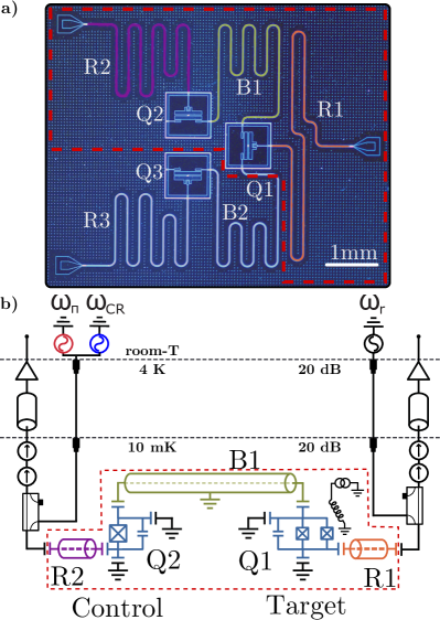
Figure 1: (color online) (a) False color optical micrograph of the device with the qubits and resonators used in the experiment outlined in red. (b) Circuit schematic.

To measure the state of each qubit, we employ an autodyne measurement Ryan et al. (2015) of the resonator reflection where the state of the qubit is imprinted on the dispersive shift of its corresponding readout resonances. Drive and measurement tones are shaped using custom arbitrary waveform generators (APS) available from Raytheon BBN BBN . Microwave signals are sent to the CPW readout resonators through directional couplers. The reflected signals pass through a series of microwave isolators before being amplified by a HEMT at the 3K stage. The signals are then further amplified at room temperature before being down converted with a doubly-balanced mixer and digitized by an Alazar ATS9870 data acquisition card.

We perform spectroscopy on R1 and R2 to identify the qubit transition frequencies (Fig. 2). For Q2, we observe $\omega_{ge}^{Q2}/2\pi=4.349\,{\rm GHz}$ with an anharmonicity $\delta_{2}/2\pi=(\omega_{ge}^{Q2}-\omega_{ef}^{Q2})/2\pi=-360\,{\rm MHz}$. We then step through the applied magnetic flux $\Phi_{Q1}$ to follow the variation in transition frequency for split-junction qubit Q1. The qubit has an upper, flux-insensitive sweet spot at $\omega_{ge}^{Q1}=5.786\,{\rm GHz}$ and an anharmonicity $\delta_{1}/2\pi=-347\,{\rm MHz}$. The modulation allows $\omega_{ge}^{Q1}$ to be adjusted to various detunings around $\omega_{ge}^{Q2}$. We extract a qubit-qubit coupling $J/2\pi=1.08\,{\rm MHz}\pm 0.1\,{\rm MHz}$ by tuning the qubits on resonance with each other and observing their anticrossing in spectroscopy Majer et al. (2007) (Fig. 2).

An energy relaxation time $T_{1}=57\,\mu{\rm s}$ and dephasing time $T_{2}^{*}=7.8\,\mu{\rm s}$ were observed for Q2. The short dephasing time is likely due to the large charging energy $E_{C}$ and the associated enhanced sensitivity to charge noise Koch et al. (2007). A $\sim$400 kHz charge splitting was observed in spectroscopy for Q2. For Q1, we measure $T_{1}=50\,\mu{\rm s}$ and $T_{2}^{*}=2.8\,\mu{\rm s}$ on average in the region where our experiments were performed. The reduced dephasing time of Q1 can be attributed to its sensitivity to magnetic flux noise at the bias points far from the flux-insensitive sweetspot where our experiment was conducted.

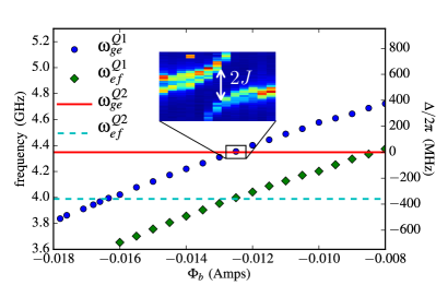
Figure 2: Spectroscopy showing the flux-modulation of the tunable qubit (Q1) above and below the fixed-frequency qubit (Q2). The inset shows the avoided crossing between the two qubits. From this we extract a $J/2\pi$ coupling of $1.08\,{\rm MHz}$ between the qubits. Horizontal lines denote the 0-1 transition frequency $\omega_{ge}$ (solid red) and the 1-2 transition frequency $\omega_{ef}$ (dashed blue) of Q2.

IV IV. Measurements of Cross Resonance

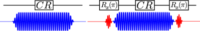
Figure 3: (color online) Pulse schematic showing the CR drive signals with the control in the ground (left) and excited (right) state.

Following our spectroscopic map of the two qubits, we move the tunable qubit to a specific detuning and apply a microwave pulse of frequency $\omega_{ge}^{Q1}(\Phi_{b})/2\pi$ to the drive line of Q2. To see the CR effect, we perform a Rabi-style measurement where we scan through the pulse width for the microwave signal at $\omega_{ge}^{Q1}(\Phi_{b})/2\pi$ applied to the drive line coupled to Q2 with no pulses applied at $\omega_{ge}^{Q2}/2\pi$(Fig. 3). Thus, Q2 ideally remains in its ground state during the sequence. We then repeat this measurement, but with a $\pi$-pulse applied to Q2 with the microwave generator tuned to $\omega_{ge}^{Q2}/2\pi$ before and after the CR pulse (Fig. 3). This drives Q2 into its first excited state before the application of the CR pulse and returns Q2 to the ground state after the CR pulse. Immediately following this pulse sequence, the state of Q1 is readout through its readout resonator. Rabi oscillations of Q1 are plotted in (Fig. 4) verse drive power. The sweep of CR drive power allows us to extract the quantity $\mu$ which will be detailed in the next section. We then repeat this process while stepping through applied magnetic flux to vary the qubit-qubit detuning $\Delta/2\pi=(\omega_{ge}^{Q1}(\Phi_{b})-\omega_{ge}^{Q2})/2\pi$.

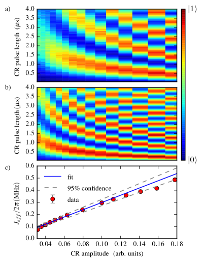
Figure 4: (color online) Measurements of Rabi oscillations of the target qubit during the CR drive for both states of the control qubit at $\Delta=-78\,{\rm MHz}$. (a) Density plot showing the probability of finding the target qubit Q1 in the excited state as a function of CR pulse amplitude and duration. (b) Density plot showing the probability of finding the target qubit Q1 in the excited state as a function of CR pulse amplitude and duration but with a $\pi$ pulse applied before and after the CR pulse. (c) Plot of $J_{\mathrm{eff}}/2\pi$ vs CR pulse amplitude from figures (b) and (a) as described in the text with a fit to the linear regime. The dashed lines correspond to 95% confidence intervals on the fit for the given data.

V V. Analysis

At each detuning we analyze the CR data by fitting damped sinusoids to the oscillations for each drive amplitude via the least-squares method. Subtracting the extracted oscillation frequencies from the traces with and without $\pi$-pulses on the control qubit, we obtain twice the CR interaction strength for each drive amplitude.

$$\begin{split}J_{\mathrm{eff}}/2\pi=\frac{f_{Rabi}^{\pi}-f_{Rabi}}{2}\end{split}$$ (8)

The frequency difference is twice $J_{\mathrm{eff}}$ since the target qubit rotates in the opposite direction and at equal rates dependent on the state of the control qubit. At low powers the CR response is linear in drive amplitude. The frequency difference at low drive amplitude is plotted in (Fig 4c) for a detuning of $-78\,{\rm MHz}$. This linear response is plotted for other values of $\Delta$ in (Fig. 5) where we plot $J_{\mathrm{eff}}$ at three different detunings, one corresponding to a fast CR rate, another to a slow CR rate and a third to a CR rate with the opposite sign. In general, we observe a linear increase in $J_{\mathrm{eff}}$ for small amplitudes, followed by a saturation at larger amplitudes, similar to the behavior in Ref. Chow et al. (2011). However, the slope at small amplitudes and the magnitude of the saturation value of $J_{\mathrm{eff}}$ depend strongly on $\Delta$.

In (Fig 5) we clearly see an drop in $J_{\mathrm{eff}}$ to a small value before recovering and behaving more erratically. The dip in $J_{\mathrm{eff}}$ was observed in all traces of $J_{\mathrm{eff}}$ (Fig. 5) that reached saturation. Similar behavior was observed in numerical simulations but was very sensitive to the choice of parameters making direct comparison impossible. Further theory of the CR effect at high drive power has been undertaken Tripathi et al. (2019) which might explain this behavior with leakage being a likely cause.

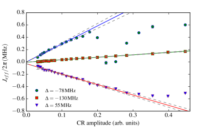
Figure 5: (color online) Plots of $J_{\mathrm{eff}}$ vs. amplitude for three select detunings with fast, slow and negative CR. Error bars for the points indicate uncertainty in the frequency difference while the dashed grey lines indicate 95% confidence intervals for the slope in the linear region.

The slope of a linear fit to $J_{\mathrm{eff}}$ at small amplitudes yields the CR parameter $\mu$. Extracting $\mu$ at each $\Delta$ we obtain a plot of the CR rate vs. qubit-qubit detuning (Fig. 6). The error bars correspond to the 95% confidence intervals on the linear slope in the low amplitude regime which are the dashed lines in (Fig. 5).

To relate these slopes to Eq. (LABEL:mu), we need to normalize them by a quantity capturing the drive susceptibility of the control qubit. To this end, the data points in (Fig. 7) are scaled by a single best fit parameter to the theory curve. For this data a value of 75.5 MHz/amp was found. The values of the theory curve are well known since the chip parameters needed to calculate it are easily measured experimental quantities, in this case the always-on $J$ coupling, control qubit anharmonicity and the qubit-qubit detuning. An analysis of the drive line and electronics predicted a value of $\sim$98 MHz/amp. This is 20% from the estimated value showing the fitted parameter it to be reasonable.

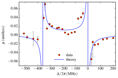
Figure 6: (color online) Plot of the extracted $\mu$ values. The error bars are the confidence intervals from (Fig. 5). Theoretical curve for $\mu$ vs. detuning from Eq.(LABEL:mu) with data scaled by a factor computed as described in text.

In addition to extracting $\mu(\Delta)$ from the $J_{\mathrm{eff}}$ plots, we also measure the CR saturation rate for each $\Delta$ by fitting a line with zero slope to the asymptotic level of $J_{\mathrm{eff}}$ for large amplitudes. This corresponds to the quickest the CR interaction can be driven in practical experiments for a given chip and detuning. Figure 7 shows the saturation rate vs. $\Delta$. Regions near the control qubit’s 0-1 transition and its anharmonicity tend to saturate at the highest rates. This is consistent with the measured $\mu$ values as the two should be roughly correlated. In contrast to $\mu$ there is no analytic expression for the saturation rate, making further analysis difficult though it shouldn’t be faster than the bare couping $J$ between qubits.

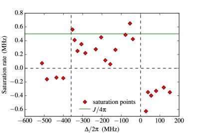
Figure 7: (color online) Saturation rate vs. detuning extracted from the $J_{\mathrm{eff}}$ plots. Dashed lines show the $\Delta=0\,{\rm MHz}$ and $\Delta=360\,{\rm MHz}$ points as well as a line to indicate $J_{\mathrm{eff}}=0$. The green line denotes the bare coupling $J$ between the qubits when tuned in resonance with each other.

VI VI. Conclusions

In conclusion, we have explored the CR effect as a function of qubit-qubit detuning. This work represents the first systematic study of CR vs. $\Delta$ on a single chip. We find good agreement between the experimental data and a model accounting for the higher energy levels of the transmon. This work will help guide future chip design by highlighting regions where the CR rate can be increased by controlling the relative detuning between qubits in a mulit-qubit system. With increasing qubit density and chip complexity, a clear understanding of this aspect of frequency space will only become more important.

VII Acknowledgments

We thank M. B. Rothwell and G. A. Keefe for fabricating devices. This research was funded by the Office of the Director of National Intelligence (ODNI), Intelligence Advanced Research Projects Activity (IARPA), through the Army Research Office under grant No. W911NF-10-1-0324. All statements of fact, opinion or conclusions contained herein are those of the authors and should not be construed as representing the official views or policies of IARPA, the ODNI, or the U.S. Government. Some of the preliminary device fabrication involved the use of the Cornell NanoScale Facility, a member of the National Nanotechnology Infrastructure Network, which is supported by the National Science Foundation (Grant ECS-0335765).

References

- Clarke and Wilhelm (2008) J. Clarke and F. K. Wilhelm, Nature 453, 1031 (2008).
- Devoret and Schoelkopf (2013) M. H. Devoret and R. J. Schoelkopf, Science 339, 1169 (2013).
- Chow et al. (2014) J. M. Chow, J. M. Gambetta, E. Magesan, D. W. Abraham, A. W. Cross, B. R. Johnson, N. A. Masluk, C. A. Ryan, J. A. Smolin, S. J. Srinivasan, and M. Steffen, Nat Commun 5:4015 (2014).
- Barends et al. (2014) R. Barends, J. Kelly, A. Megrant, A. Veitia, D. Sank, E. Jeffrey, T. C. White, J. Mutus, A. G. Fowler, B. Campbell, Y. Chen, Z. Chen, B. Chiaro, A. Dunsworth, C. Neill, P. O’Malley, P. Roushan, A. Vainsencher, J. Wenner, A. N. Korotkov, A. N. Cleland, and J. M. Martinis, Nature 508, 500 (2014).
- Córcoles et al. (2015) A. Córcoles, E. Magesan, S. J. Srinivasan, A. W. Cross, M. Steffen, J. M. Gambetta, and J. M. Chow, Nat Commun 6 (2015).
- Fowler et al. (2012) A. G. Fowler, M. Mariantoni, J. M. Martinis, and A. N. Cleland, Phys. Rev. A 86, 032324 (2012).
- Rigetti and Devoret (2010) C. Rigetti and M. Devoret, Phys. Rev. B 81, 134507 (2010).
- Paraoanu (2006) G. S. Paraoanu, Phys. Rev. B 74, 140504 (2006).
- Chow et al. (2011) J. M. Chow, A. D. Córcoles, J. M. Gambetta, C. Rigetti, B. R. Johnson, J. A. Smolin, J. R. Rozen, G. A. Keefe, M. B. Rothwell, M. B. Ketchen, and M. Steffen, Phys. Rev. Lett. 107, 080502 (2011).
- Córcoles et al. (2013) A. D. Córcoles, J. M. Gambetta, J. M. Chow, J. A. Smolin, M. Ware, J. Strand, B. L. T. Plourde, and M. Steffen, Phys. Rev. A 87, 030301 (2013).
- Majer et al. (2007) J. Majer, J. M. Chow, J. M. Gambetta, J. Koch, B. R. Johnson, J. A. Schreier, L. Frunzio, D. I. Schuster, A. A. Houck, A. Wallraff, A. Blais, M. H. Devoret, S. M. Girvin, and R. J. Schoelkopf, Nature 449, 443 (2007).
- Gambetta (2013) J. Gambetta, IFF Spring School 2013 Quantum Information Processing Lecture Notes 339, Chap. B4 (2013).
- Magesan and Gambetta (2018) E. Magesan and J. M. Gambetta, (2018), arXiv:1804.04073 .
- de Groot et al. (2012) P. C. de Groot, S. Ashhab, A. Lupaşcu, L. DiCarlo, F. Nori, C. J. P. M. Harmans, and J. E. Mooij, New Journal of Physics 14, 073038 (2012).
- Patterson et al. (2019) A. D. Patterson, J. Rahamim, T. Tsunoda, P. Spring, S. Jebari, K. Ratter, M. Mergenthaler, G. Tancredi, B. Vlastakis, M. Esposito, and P. J. Leek, (2019), arXiv:1905.05670 .
- Koch et al. (2007) J. Koch, T. M. Yu, J. Gambetta, A. A. Houck, D. I. Schuster, J. Majer, A. Blais, M. H. Devoret, S. M. Girvin, and R. J. Schoelkopf, Phys. Rev. A 76, 042319 (2007).
- Schreier et al. (2008) J. A. Schreier, A. A. Houck, J. Koch, D. I. Schuster, B. R. Johnson, J. M. Chow, J. M. Gambetta, J. Majer, L. Frunzio, M. H. Devoret, S. M. Girvin, and R. J. Schoelkopf, Phys. Rev. B 77, 180502 (2008).
- Ryan et al. (2015) C. A. Ryan, B. R. Johnson, J. M. Gambetta, J. M. Chow, M. P. da Silva, O. E. Dial, and T. A. Ohki, Phys. Rev. A 91, 022118 (2015).
- (19) https://www.raytheon.com/capabilities/products/quantum.
- Tripathi et al. (2019) V. Tripathi, M. Khezri, and A. N. Korotkov, (2019), arXiv:1902.09054 .