LOCAL TIME STEPPING METHODS AND DISCONTINUOUS GALERKIN METHODS APPLIED TO DIFFUSION ADVECTION REACTION EQUATIONS

Abstract

This paper is focussed on the numerical resolution of diffusion advection and reaction equations (DAREs) with special features (such as fractures, walls, corners, obstacles or point loads) which globally, as well as locally, have important effects on the solution. We introduce a multilevel and local time solver of DAREs based on the discontinuous Galerkin (DG) method for the spatial discreization and time stepping methods such as exponential time differencing (ETD), exponential Rosenbrock (EXPR) and implicit Euler (Impl) methods. The efficiency of our solvers is shown with several experiments on cyclic voltammetry models and fluid flows through domains with fractures.

Keywords Local time stepping methods  $\cdot$ discontinuous Galerkin method  $\cdot$ implicit Euler method  $\cdot$ exponential time differencing method  $\cdot$ exponential Rosenbrock method  $\cdot$ diffusion advection and reaction  $\cdot$ cyclic voltammetry  $\cdot$ domain with fracture  $\cdot$ unstructured mesh

1 Introduction

We examine numerical methods for diffusion advection and reaction equations of the form

$$\dfrac{\partial C}{\partial t}-\nabla\cdot(D\nabla C)+\nabla\cdot\textbf{v}C=R(C),\text{ given }C(x,0)=C_{0}(x),\quad x\in\Omega,$$ (1)

where, for example, $C$ is a concentration of a solute, where $R(C)$ is a reaction term, $D$ is a diffusivity and v is a given velocity. Often, there are special features (e.g. fractures, walls, corners, obstacles, electrodes, point loads or irregular material interfaces), which affect locally the flow and transport of the solute. To accurately capture such local behaviour numerically, spatial local refinement is necessary. However, this requires a reduction of the time step, $\Delta t$, for stability (while using the explicit time integrator) and for accuracy (while using both explicit and implicit time integrators). Unfortunately, when applied uniformly on all the simulation domain, $\Omega$, the reduced time step leads to an unacceptable large CPU time, making the use of local time stepping (LTS) methods highly desirable. The key feature of LTS methods is to split the solution domain $\Omega$ into several sub-domains $\Omega_{i}$ each with a time step $\Delta t_{i}$ as large as possible for efficiency. According to [28], a LTS method is efficient if it ensures accuracy of the solution, i.e. the solution has to be more accurate than the one obtained with a global coarse mesh, and in addition leads to reduced CPU time compared to the one obtained when using a small time step on the whole domain. We give a short review of LTS methods in the context of the DG applximation.

The LTS methods have their roots in the work of Rice [49], who in 1960 developped the so-called multirate Runge-Kutta methods for a two scale system of ordinary differential equations (ODEs). The multirate approach, for ODEs, was then combined with linear multistep integrators in 1984 by Gear et al. [37] to improve the accuracy; and their stability properties were analyzed in 1989 by Skelboe et al [53]. These multirate methods were based on the static partitioning of the domain $\Omega$ generated from the priori knowledge of the physics of the problem. This limitation was overcomed in 1997 by Engstler et al. [22] when they introduced the multirate extrapolation methods for ODEs, based on Richardson extrapolation. Due to their unconditional stability, the (DG) method was also used to handle the time refinement of ODEs. The DG method, denoted DG($q$) while using the polynomials of degree $q\in\mathbb{N}$, applied to ODEs was first studied in 1974 by LeSaint et al. [43]. It was proven to be strongly A-stable of order $2q+1$ by the authors. Note that the case $q=0$ is equivalent to implicit Euler scheme. Adaptive error control was introduced in [39] and more recently considered in [25, 4]. For more insight on the DG method applied to ODEs, see for example [8].

In the case of partial differential equations (PDEs), several schemes using the DG method have been developed to handle space and time refinement problems. The finite element (FE) method in space followed by the DG method in time was used in [1, 7, 6, 23, 24, 26, 51, 52] to solve parabolic problems and extended in [31] to a linear nonstationary convection-diffusion-reaction problem. This method, denoted CG($p$)DG($q$), used a piecewise polynomials of degree $p$ and $q$ respectively for the space and time discretization. Feistauer et al. [32] proposed the theory of error estimates for CG($p$)DG($q$) applied to a nonstationary convection-diffusion problem with a nonlinear convection and linear diffusion. The DG method is used in both space and time by Feistauer et al. [5, 33, 19] to solve the nonstationary parabolic problems with nonlinear convection and diffusion.

Other than the DG time discretization, Lörcher et al. [44] used the LTS method (denoted ADER-DG) based on arbitrary high-order derivatives methods and allowed every element of the mesh to have its own time-step, which is dictated by the element size. The ADER-DG schemes, as presented for electromagnetism [55] and elastic wave propagation in [21], were obtained by the extension to the DG framework, of the ADER finite volume (ADER-FV) approach which was developed by Toro et al. [56]. The ADER-DG scheme was used by Fambri et al. [30] on space-time adaptive meshes for compressible Navier-Stokes equations and the equations of viscous and resistive magnetohydrodynamics in two and three space-dimensions. Angulo et al. [2] introduced the LTS schemes (denoted LTS-LF) based on the leapfrog (LF) and Runge-Kutta (RK) time integrators, where the mesh is sorted into different sub-domains with appropriate time step on each. In 2009, Diaz and Grote introduced an energy-conserving LTS-LF scheme [17] for the acoustic wave equation, which they extended in 2015 into a multi-level version [18]. Rietmann et al. [50] developed a new LTS method based on the Newmark scheme for large scale wave propagation, which also can be extended to accommodate multiple sub-domains of mesh refinement.

Unfortunately, the DG method in space and time considered in [5, 33, 19, 44, 2, 17, 18, 50] were still special, since they always had boundaries in time aligned with the time direction i.e. the spatial boundaries are independent of the time. To overcome this limitation, an alternative space-time DG method was introduced by van der Vegt et al. in [15, 16] for inviscid compressible flows and extended in [40] to the compressible Navier-Stokes equation. The key feature of this space-time DG method is that no distinction is made between space and time variables and the DG discretization is directly and simultaneously performed in space and time. This then provides flexibility to deal with time dependent boundaries, deforming elements and naturally results in a conservative discretization, even on deforming, locally refined meshes with hanging nodes. A complete hp-error and stability analysis of the space-time DG discretization for the linear advection-diffusion equation is given in [54].

However, the bottleneck of these LTS methods, based on the DG discretization, is that they lead to a large discrete problem in space-time, especially in the presence of complex geometry or localized small-scale physics. As a consequence, they can become very expensive in terms of storage and computational time. Thus, we focus on splitting the solution domain on several small regions, yielding several low dimension system of ODEs from the DG spatial discretization, which can then be solved separately. We look at two approaches: the first based on [3, 45, 58, 20, 42, 57] where the sub-domains are overlapped and the second using non-overlapping sub-domains based on [13, 12, 14]. Let us denote by GTS-DG, the global time stepping solver of the DAREs that combines the DG method and a time integrator with unique time step on the entire solution domain.

The format of this paper is as follows. In Section 2, we describe our proposed LTS-DG schemes. Various numerical results are presented in Section 3 to validate and compare the efficiency of the proposed LTS-DG schemes against GTS-DG schemes, and the conclusion follows in Section 4.

2 LTS-DG schemes

We construct our LTS-DG schemes by combining domain decomposition techniques, the DG spatial discretization and the time integrators. The approach follows three basic steps:

1. We use a priori knowledge of the local behaviour of the solution due to fractures, walls, corners, obstacles, point loads, etc, to construct a refined mesh of the spatial domain. For example, this is illustrated in Figure 1 (a) by showing the refined mesh for the domain with fracture.

2. We choose the local time step on each element of the mesh such that it is proportional to the element size (similar to [44]) and inversely proportional to the norm of the fluid velocity v (if it is different from zero). This splits the solution domain, $\Omega$, into sub-domains, $\Omega_{i}$ with the local time steps $\Delta t_{i}$ for all $i\in\{0,\cdots,m\}$.

3. Finally, we use either interpolation or extrapolation techniques to estimate the solution at the internal boundary, $\Gamma_{i}$, given by

   $$\Gamma_{i}=\partial\Omega_{i}\setminus\partial\Omega,$$ (2)

   for all $i\in\{0,\cdots,m\}$. So, one can solve the PDEs independently on each sub-domains, $\Omega_{i}$, using the DG method combined with the standard time integrators and local time step $\Delta t_{i}$.

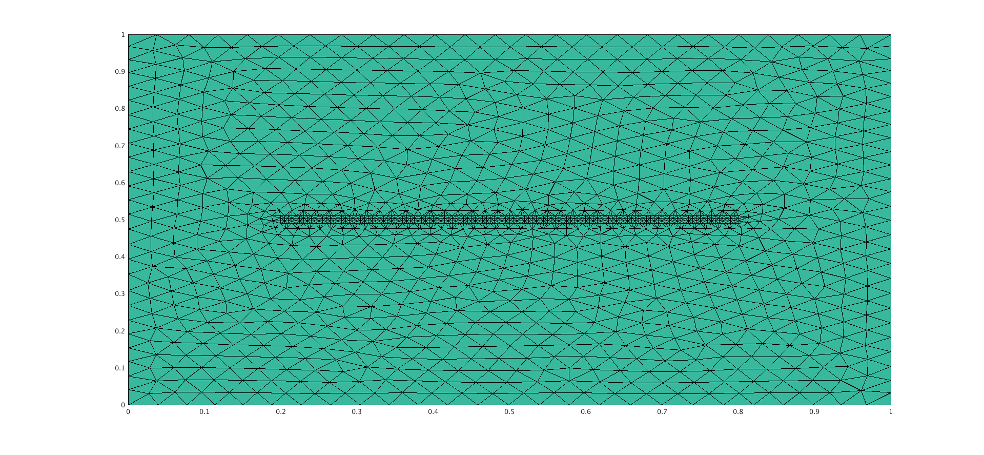
(a)

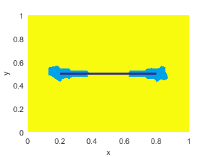
(b)

Figure 1: (a) Unstructured mesh of domain with fracture using $distmesh2d$. (b) Sub-domains: $\Omega_{0}$ (black), $\Omega_{1}$ (blue) and $\Omega_{2}$ (yellow).

We now look at these steps in more details. The first step can be implemented, for example, using the MATLAB’s code $distmesh$ [48, 47]. We complete the second step by assuming that, beside being proportional to the element size and inversely proportional to the norm of the fluid velocity, the local time step on the sub-domain $\Omega_{i}$ is given by

$$\Delta t_{i}=\lambda_{i}\times\Delta t,$$ (3)

with $\lambda_{i}\in\mathbb{N}$, for a given $\Delta t\in\mathbb{R}^{+}$ and all $i\in\{0,\cdots,m\}$. Thus, for a given initial time $T^{0}$ and final time $T^{1}$, we have a time synchronization over all sub-domains at some time $t\in[T^{0},T^{1}]$. We illustrate how this can be achieved, in two dimension case, ensuring that the CFL condition is satisfied on each element $E$ of the triangulation. Let

$$\Delta t_{E}=2^{-\mathbf{N}^{E}},\;\;\;\;\mathbf{N}^{E}=\lceil\log_{2}\left(\frac{\parallel\textbf{v}^{E}\parallel}{R_{E}\mathbf{C}_{max}}\right)\rceil,$$ (4)

where $\lceil\cdot\rceil$ is the ceiling function [38], $\mathbf{C}_{max}\in\mathbb{R}$ is the Courant number [10], $R_{E}$ is the radius of the incircle of the element $E$. This ensures that the CFL condition is verified on each element $E$. 4 yields the decomposition of the global solution domain, $\Omega$, into sub-domains $\Omega_{i},i\in\{0,\cdots,m\}$ defined as follows

$$\Omega_{i}=\{E\in\mathcal{T}_{h}\text{ such that }\Delta t_{E}=\Delta t_{i}\},$$ (5)

where $\Delta t_{i}$ is a fixed value in $\mathbb{R}$ for a given value of $i$ in $\{0,\cdots,m\}$. The synchronized time $t=t^{n}$ while advancing locally the solution from $T^{0}$ are given by

$$t^{n}=T^{0}+n\times\Delta t_{\max},\;\text{ with }\;\Delta t_{\max}=\max\{\Delta t_{i},i=0,\cdots,m\}.$$ (6)

The sub-domains, obtained when we applied the second step to the fracture problem, are illustrated in Figure 1(b). Note from Figure 1(b) that $m=2$ with the sub-domains $\Omega_{0},\Omega_{1}$ and $\Omega_{2}$ respectively represented by the color black, blue and yellow. One can also see that the sub-domain $\Omega_{1}$ is the union of two disjoint regions while its interior boundary $\Gamma_{1}$ is shared with the sub-domains $\Omega_{0}$ and $\Omega_{2}$. Once the sub-domains are defined, the large time-dependant system of ODEs, obtained from the DG space discretization of the DAREs on the $\Omega$, can then be split into $m+1$ smaller systems of ODEs, denoted $\text{SO}_{i}$ for all $i\in\{0,\cdots,m\}$, given by

$$(\text{SO}_{i}):\;\;\mathbb{M}_{i}\frac{d}{dt}X_{i}+\mathbb{S}_{i}X_{i}=\mathbb{F}_{i}+\mathbb{B}_{i}+\mathbb{S}_{i}^{e}X_{i}\Bigr{|}_{\Gamma_{i}}\;\text{ on }\;\Omega_{i}\times[0,T].$$ (7)

Here, $X_{i}$, $\mathbb{S}_{i},\mathbb{M}_{i}$, $\mathbb{F}_{i}$ and $\mathbb{B}_{i}$ respectively represent the local solution, stiffness matrix, the mass matrix, source term and the contribution of the global boundary condition on the sub-domain $\Omega_{i}$. The matrix $\mathbb{S}_{i}^{e}$ is used to weakly enforce the internal boundary condition. Therefore, the sum of the last two terms at the right hand side of 7 enforces the local boundary condition on $\partial\Omega_{i}$. Because the interior penalty discontinuous galerkin (IP-DG) method is compact and the global mass matrix obtained from the IP-DG spatial discretization is either block-diagonal or diagonal, see [59], then the local entities $X_{i}$, $\mathbb{S}_{i},\mathbb{M}_{i}$, $\mathbb{S}_{i}^{e}$, $\mathbb{F}_{i}$ and $\mathbb{B}_{i}$ can be easily extracted from their global values. An example of this extraction is shown in Subsection 3.2.

Let us introduce the following notation

$$t_{i}^{j}=T^{0}+j\times\Delta t_{i},\qquad s_{i}=\frac{T^{1}-T^{0}}{\Delta t_{i}},\qquad X_{i}^{j}=X_{i}\Bigr{|}_{t=t_{i}^{j}},$$ (8)

for all $i\in\{0,\cdots,m\}$ and all $j\in\{0,\cdots,s_{i}\}$. If one can estimate $X_{i}^{j}\Bigr{|}_{\Gamma_{i}}$, by any means, then the local solution $X_{i}^{j}$ at time $t_{i}^{j}$ can be obtained from its initial value $X_{i}^{0}$, by applying the time integrator schemes to the local system $\text{SO}_{i}$ given by Equation 7, with the uniform local time step $\Delta t_{i}$.

As a consequence, the construction of our LTS-DG schemes is reduced to finding a way to estimate the component $X_{i}^{j}\Bigr{|}_{\Gamma_{i}}$ at any time $t_{i}^{j}$ for all $i\in\{0,\cdots,m\}$ and all $j\in\{0,\cdots,s_{i}\}$. We only need to describe the LTS-DG schemes to advance the global solution $X$, on the solution domain $\Omega$, from its known value at the synchronized time $t^{n}$ (as it happens at the initial time $T^{0}$) to the synchronized time $t^{n+1}$. The process can then be repeated, in order to estimate the global solution $X$ at the final time $T^{1}$ from the global solution $X^{0}$ at the initial time $T^{0}$. Next, in Subsection 2.1 and Subsection 2.2, we described two different techniques respectively refer as overlap LTS-DG and non-overlap LTS-DG methods to locally advance the solution from synchronized time $t^{n}$ to $t^{n+1}$.

2.1 Overlap LTS-DG schemes (OLTS-DG)

The key idea of the proposed overlap LTS-DG methods, denoted OLTS-DG, is to overlap the different sub-domains obtained from the decomposition of the solution domain $\Omega$, in order to extrapolate the components $X_{i}^{j}\Bigr{|}_{\Gamma_{i}}$ at any time $t_{i}^{j}$ for all $i\in\{0,\cdots,m\}$ and all $j\in\{0,\cdots,s_{i}\}$. This approach appeared in [3], where a Crank-Nicolson scheme was used for the time-space discretization of the one spatial dimension heat equation. The authors proved that without local refinement in time ($\Delta t_{i}=\Delta t$) and space ($h_{i}=h$) this scheme is stable, provided that

$$\Delta t\leq C\left(\frac{L}{\log L}\right)^{2}h^{2},$$

where $Lh$, for $L\in\mathbb{N}$, is the size of the overlap, and an error estimate of the form $O(\Delta t^{2}+h^{2})$. So, in this case, increasing the size of the overlap can reduce the stability constraint on the time step. To avoid the stability constraint, Ewing et al. [27] used a standard centred finite difference scheme in space with backward Euler in time for a linear DAREs. More recently, an approach based on domain decomposition and finite volume discretization, has been proposed by Faille et al. [29] for the one dimensional heat equation. It was used by Gander et al. [36] to investigate the one dimensional convection dominated nonlinear conservation laws.

Here, we introduce new schemes that extend this approach to the DAREs in one, two or three spatial dimensions. We use the DG method for the space discretization and time integrators such as Impl, ETD, EXPR for the resolution in time of 7, in order to avoid numerical instability.

2.1.1 Overlapping procedure of the domain solution

Once the sub-domains $\Omega_{i},\;i\in\{0,\cdots,m\}$ are obtained, we overlap them by pushing the internal boundary $\Gamma_{i}$ in the direction of the outward normal vector.

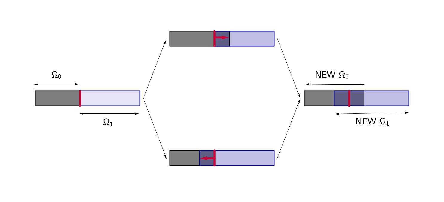
Figure 2: The procedure to overlap the regions for $\Omega=\Omega_{0}\cup\Omega_{1}$. On the left: original sub-domains $\Omega_{0}$ and $\Omega_{1}$. Middle: we push the internal boundary in the direction of the outward nornal vector. Right: new sub-domains $\Omega_{0}$ and $\Omega_{1}$

During the overlapping procedure, if any new sub-domain $\Omega_{i}$ swallows entirely another initial sub-domain $\Omega_{j}$, then we set $\Delta t_{j}=\Delta t_{i}$ so that the sub-domain $\Omega_{j}$ will be included in $\Omega_{i}$. Later on, in Subsection 3.1, we investigate numerically the effect of the size of the overlap on the accuracy of our OLTS-DG schemes.

Let us denote $\Gamma_{i,j}$ the part of the internal boundary $\Gamma_{i}$ included in the sub-domain $\Omega_{j}$ with $i\neq j$ (i.e. $\Gamma_{i,j}=\Gamma_{i}\cap\Omega_{j})$. Every time we advance the local solution $X_{j}$ on $\Omega_{j}$, we can update the $X_{i}\Bigr{|}_{\Gamma_{i,j}}$.

For a given $r\in\{1,\cdots,\frac{\Delta t_{\max}}{\Delta t}\}$, the set of eligible sub-domain $S^{r}$ is the set of sub-domains on which the known solution has to be advanced locally to the time $t^{n_{r}}=t^{n}+r\times\Delta t$. Then we have

$$S^{r}=\left\{\Omega_{i}\Bigr{|}\exists j\in\mathbb{N},t_{i}^{j}=t^{n_{r}}\right\}.$$ (9)

Note that there is a freedom in the order of which the sub-domains are updated. For example, it could either be in the increasing or decreasing order of local time step. If the time integrator $\text{INT}\in\{$Impl, ETD, EXPR $\}$ is used to advance locally the solution, we denote $DG_{\text{OLTSD-INT}}$ and $DG_{\text{OLTSI-INT}}$ the OLTS-DG scheme that updates the solution on the eligible sub-domains $S^{r}$ respectively in the decreasing and increasing order of the local time step. In Subsection 3.1, we compare the accuracy of the $DG_{\text{OLTSD-Impl}}$ and $DG_{\text{OLTSI-Impl}}$ and examine how the direction of the bulk velocity of the DAREs or the size of the overlap affect their accuracy. Unless stated, the OLTS-DG method considered for the numerical experiments is the $DG_{\text{OLTSD-INT}}$. Next, we describe step by step the algorithm of the OLTS-DG scheme, $DG_{\text{OLTSD-INT}}$, in order to advance the solution from a synchronized time $t^{n}$ to $t^{n+1}$.

2.1.2 Description of the OLTS-DG algorithm

In this section, we describe step by step the algorithm of the OLTS-DG scheme, $DG_{\text{OLTSD-INT}}$, in order to advance the solution from a synchronized time $t^{n}$ to $t^{n+1}$. To that end, we consider the overlapped sub-domains illustrated in Figure 3, where the solution domain is split into three different sub-domains (i.e. $m=2$) with the coefficient $\lambda_{i}$ in Equation 3 given by $\lambda_{i}=2^{i}$ for all $i=0,\cdots,m$. The overlapped sub-domains $\Omega_{0}$, $\Omega_{1}$ and $\Omega_{2}$ are respectively represented by the color red, blue and green. Note from Figure 3 that the internal boundaries are given by $\Gamma_{0}=\Gamma_{0,1},\;\Gamma_{1}=\Gamma_{1,0}\sqcup\Gamma_{1,2},\;\;\Gamma_{2}=\Gamma_{2,1}$.

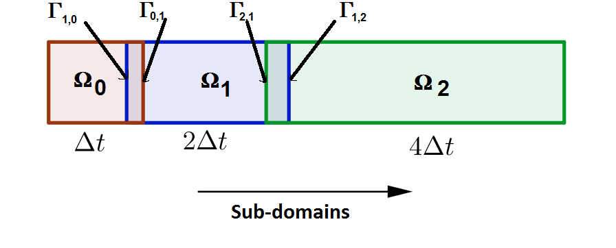
Figure 3: Overlapped sub-domains of the solution domain.

For a given time $t^{n_{r}}$, let us denote $\mathbb{X}_{i}^{n_{r}}$ and $\mathbb{X}_{i,j}^{n_{r}}$ the restriction of the global solution $X$ respectively to the internal boundaries $\Gamma_{i}$ and $\Gamma_{i,j}$ i.e.

$$\mathbb{X}_{i}^{n_{r}}=X\Bigr{|}_{\Gamma_{i},t=t^{n_{r}}},\;\;\mathbb{X}_{i,j}^{n_{r}}=X\Bigr{|}_{\Gamma_{i,j},t=t^{n_{r}}}.$$ (10)

Now let discuss step by step, how to update the solution on these interior boundaries in order to advance the solution from the synchronized time $t_{n}$ to $t_{n+1}$.

• Step one: for $r=1$, the set of eligible sub-domains is given by $S^{1}=\{{\Omega_{0}}\}$ and requires $\mathbb{X}_{0}^{n_{1}}$ to advance locally on $\Omega_{0}$ from $t^{n}$ to $t^{n_{1}}=t^{n}+\Delta t$. To that end, we then use the extrapolation $\mathbb{X}_{0}^{n_{1}}=\mathbb{X}_{0}^{n}$. The completion of this step defines $\mathbb{X}_{1,0}^{n_{1}}$, as illustrated in Figure 4 (a).

  

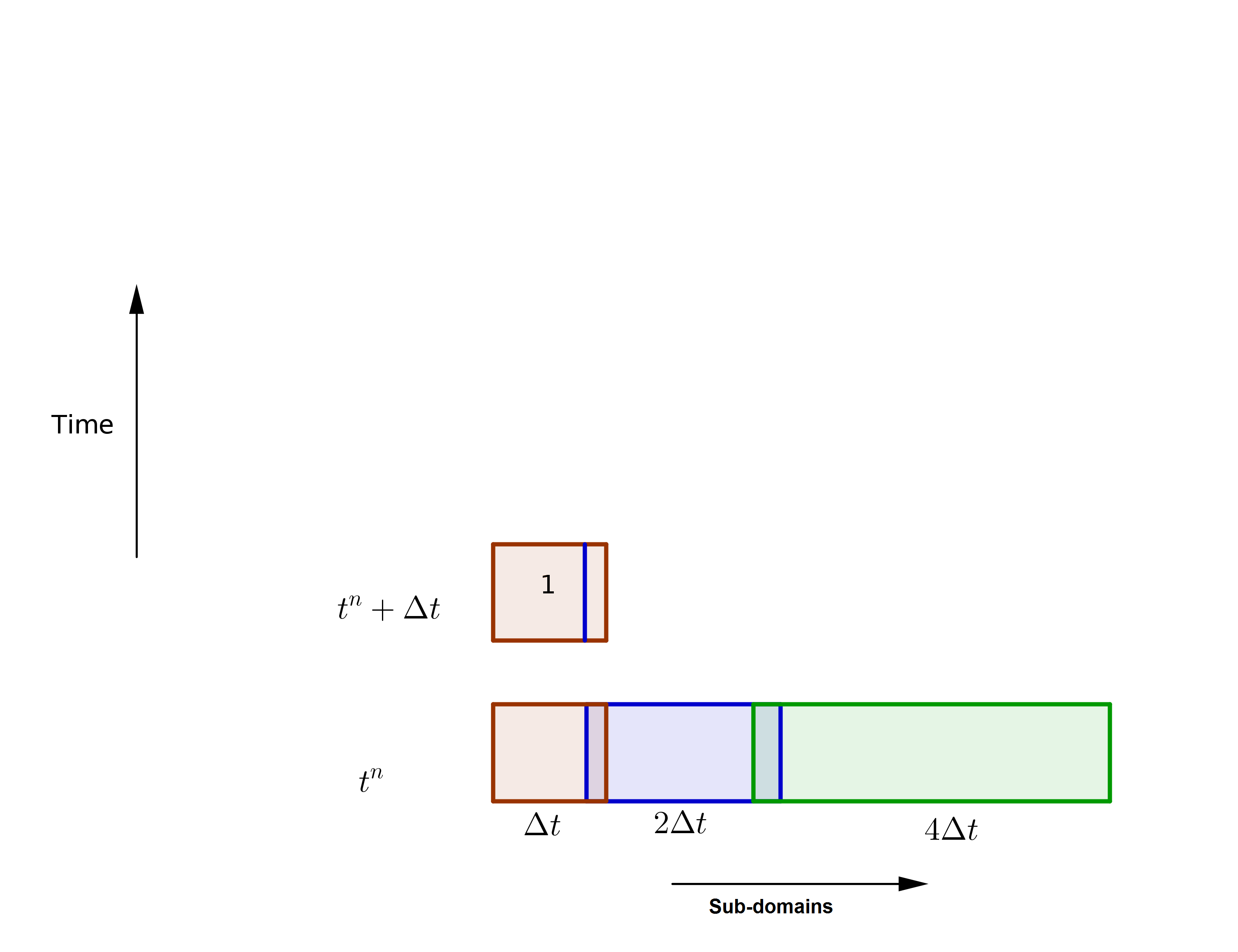
  (a)

  

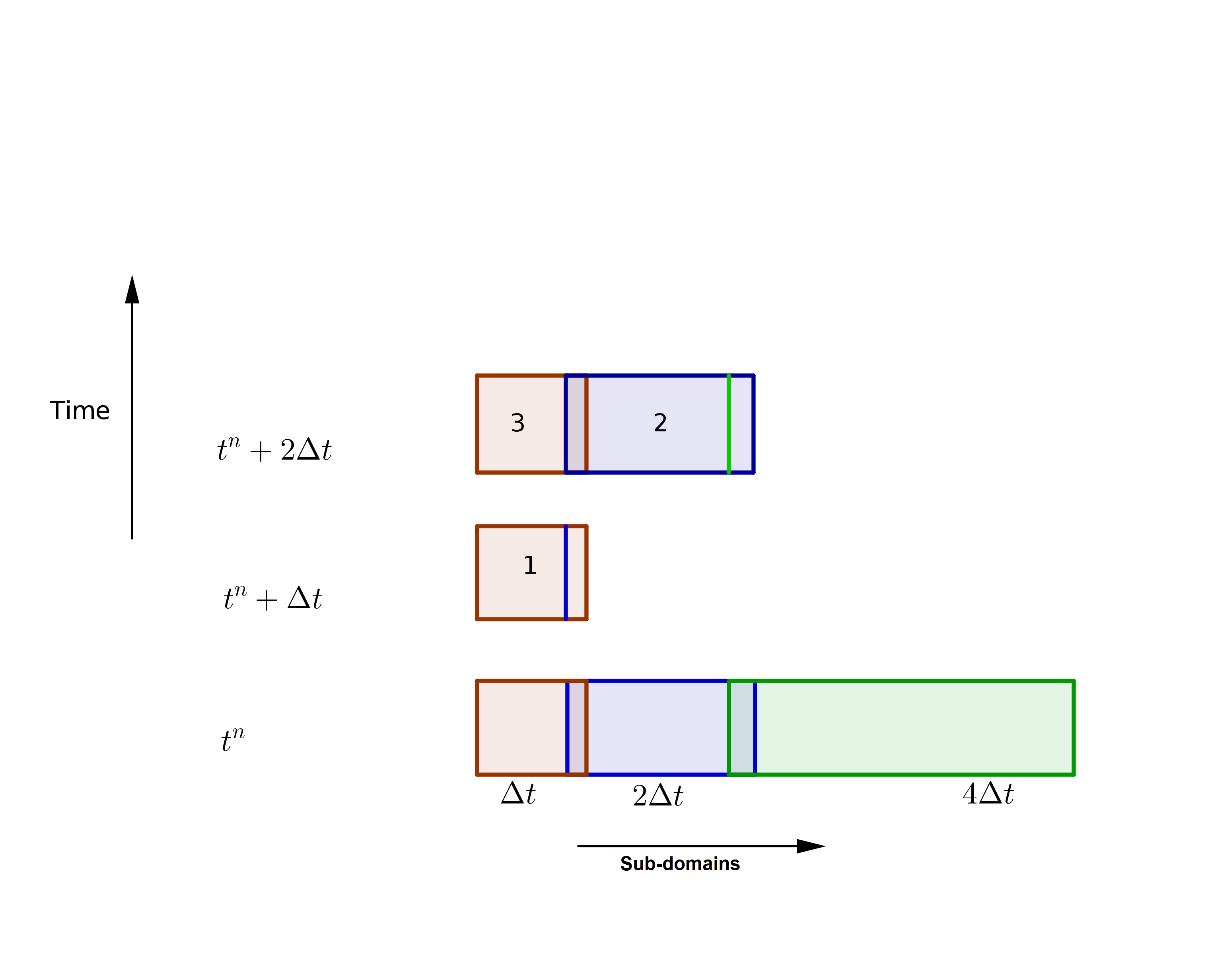
  (b)

  Figure 4: (a) The eligible solution advanced to $t^{n_{1}}$ and (b) to $t^{n_{2}}$.

• Step two: for $r=2$, the set of eligible sub-domains is given by $S^{2}=\{\Omega_{0},\Omega_{1}\}$, and we require $\mathbb{X}_{0}^{n_{2}}$ and $\mathbb{X}_{1}^{n_{2}}$ to locally advance the solution to $t^{n_{2}}=t^{n}+2\times\Delta t$. So, we first use the extrapolations $\mathbb{X}_{1,0}^{n_{2}}=\mathbb{X}_{1,0}^{n_{1}}$ and $\mathbb{X}_{1,2}^{n_{2}}=\mathbb{X}_{1,2}^{n}$ to locally advance the solution on $\Omega_{1}$ from $t^{n}$ to $t^{n_{2}}$. Note from Figure 4(b) that the completion of this simulation defines $\mathbb{X}_{0}^{n_{2}}$ and $\mathbb{X}_{2}^{n_{2}}$. We finally use $\mathbb{X}_{0}^{n_{2}}$ to advance locally the solution on $\Omega_{0}$ from $t^{n_{1}}$ to $t=t^{n_{2}}$.

• Step three: for $r=3$, the set of eligible sub-domains is given by $S^{3}=\{{\Omega_{0}}\}$ and require $\mathbb{X}_{0}^{n_{3}}$ to advance locally on $\Omega_{0}$ to $t^{n_{3}}=t^{n}+3\times\Delta t$. We use the extrapolation $\mathbb{X}_{0}^{n_{3}}=\mathbb{X}_{0}^{n_{2}}$. This is illustrated in Figure 5(a) and it shows that the completion of this step defines $\mathbb{X}_{1,0}^{n_{3}}$.

  

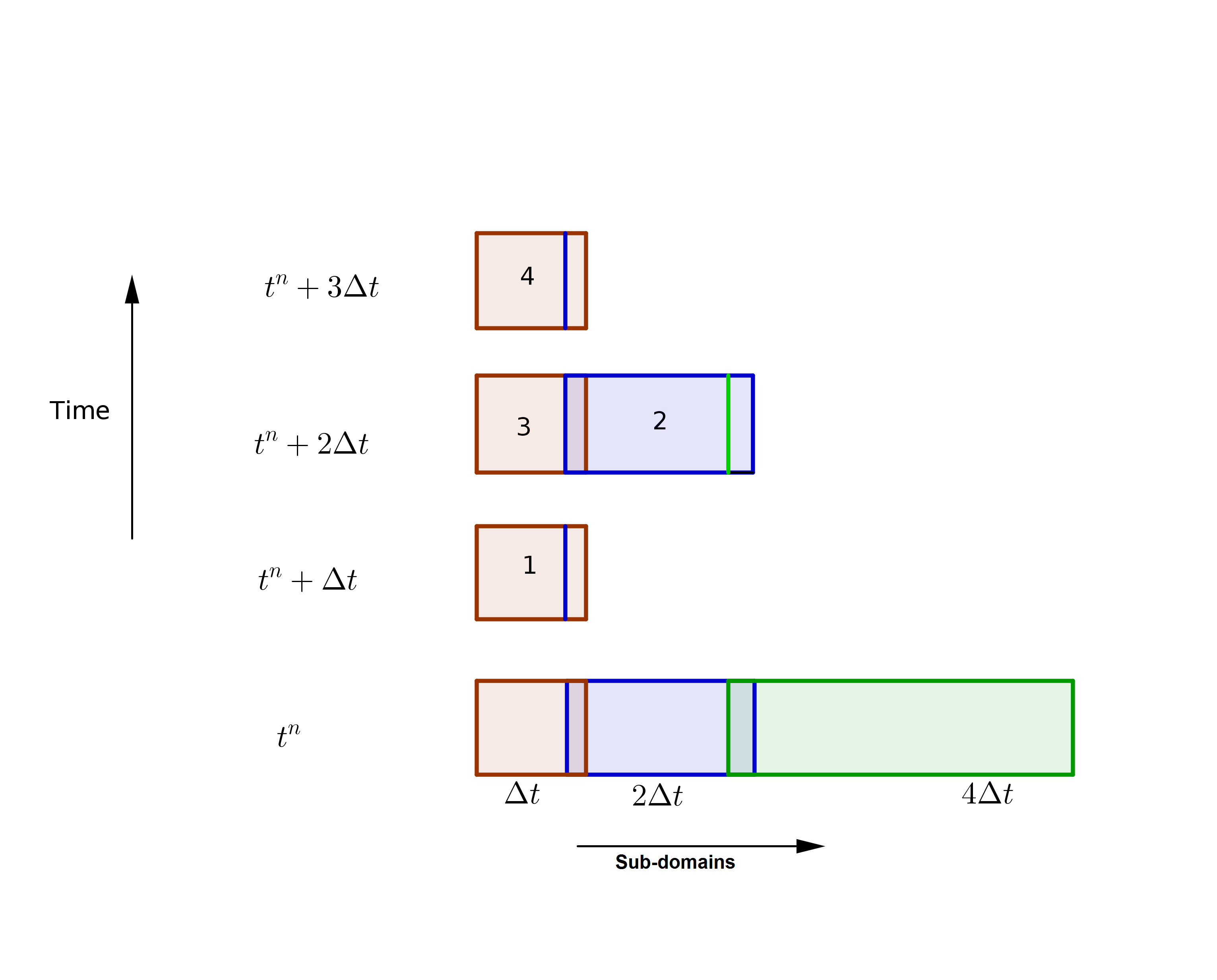
  (a)

  

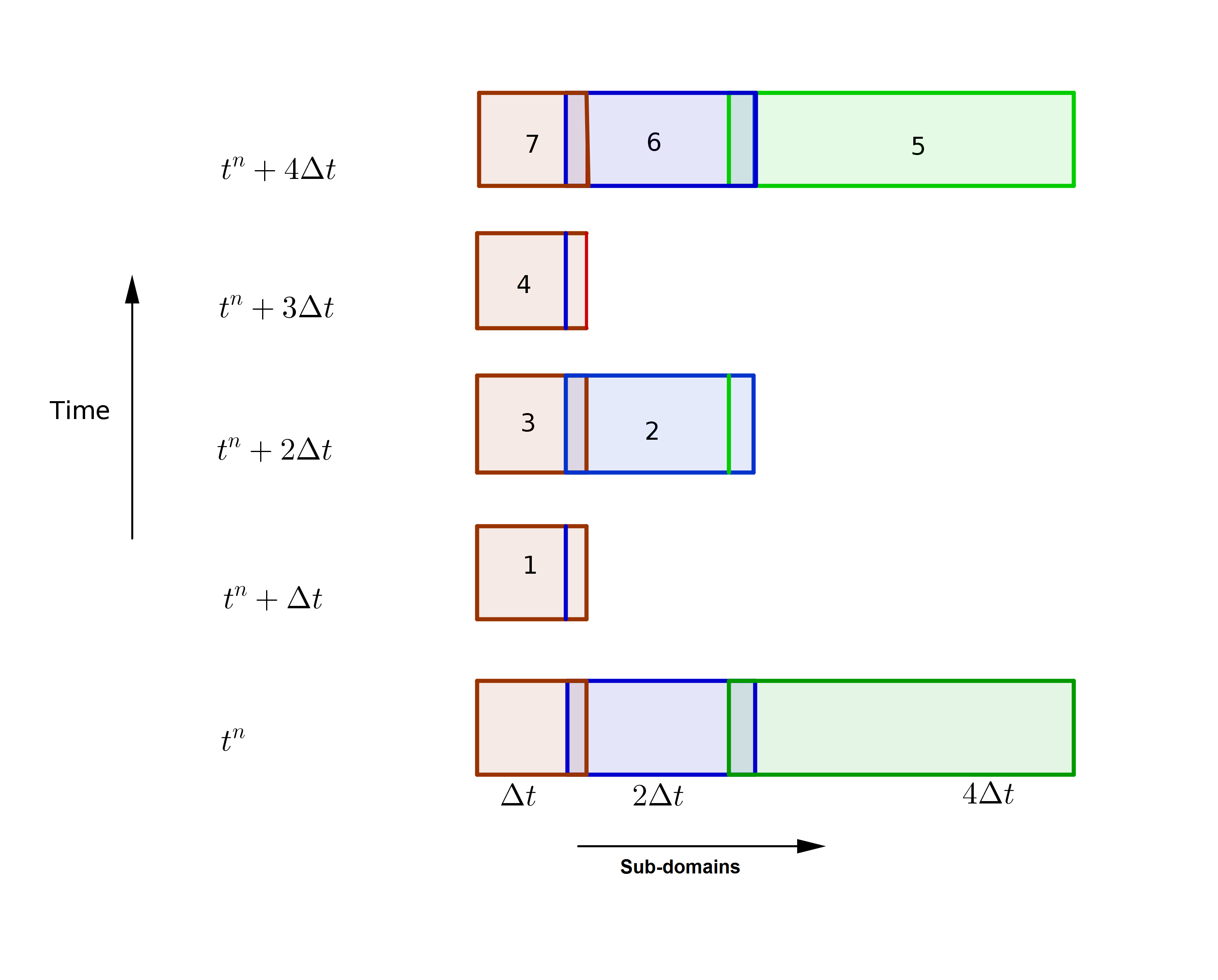
  (b)

  Figure 5: The eligible solution advanced to $t^{n_{3}}$ in (a) and $t^{n_{4}}$ in (b).

• Step four: for $r=4$, the set of eligible sub-domains is given by $S^{4}=\{\Omega_{0},\Omega_{1},\Omega_{2}\}$, and we require $\mathbb{X}_{0}^{n_{4}},\mathbb{X}_{1}^{n_{4}}$ and $\mathbb{X}_{2}^{n_{4}}$ to locally advance the solution to $t^{n_{4}}=t^{n}+4\times\Delta t$. We first locally advance the solution on $\Omega_{2}$ from $t^{n}$ to $t=t^{n_{4}}$, using the extrapolation $\mathbb{X}_{2}^{n_{4}}=\mathbb{X}_{2}^{n_{2}}$. This is illustrated in Figure 5 (b) and it shows that this simulation defines $\mathbb{X}_{1,2}^{n_{4}}$. We then use $\mathbb{X}_{1,2}^{n_{4}}$ obtained and the extrapolation $\mathbb{X}_{1,0}^{n_{4}}=\mathbb{X}_{1,0}^{n_{3}}$, to locally advance the solution on $\Omega_{1}$ from $t^{n_{2}}$ to $t^{n_{4}}$. This is also illustrated in Figure 5 (b). It shows that this simulation defines $\mathbb{X}_{0}^{n_{4}}$, which we then use to locally advance on $\Omega_{0}$ from $t^{n_{3}}$ to $t^{n_{4}}$.

At this point, the time is synchronized across the whole domain $\Omega$. By repeating this process (i.e. from step one to step four) $m^{s}=\frac{T^{1}-T^{0}}{\Delta t_{\max}}$ times, we can estimate the solution at the final time $T^{1}$, from the solution at the initial time $T^{0}$. One can implement Algorithm 1, where $S$ is the set of all overlapped sub-domains $\Omega_{i}$, $\mathbf{E}$ and $\mathbf{A}_{i}$ respectively represent the extrapolation procedure and the iterative function of the standard time integrators used to solve the local system $\text{SO}_{i}$.

Algorithm 1 Pseudo algorithm of the overlap LTS method.

for $i=0\text{ to }m-1$ do$\triangleright$ initialize the time of the known local solution $X_{i}$

     $t^{known}_{i}=T^{0}$

end for

for $n=0\text{ to }m^{s}-1$ do$\triangleright$ Loop to advance the solution from $T^{0}$ to $T^{1}$

     $t^{n}=T^{0}+j\times\Delta t_{\max}$ $\triangleright$ Compute the synchronized time $t^{n}$

     for $r=1\text{ to }\frac{\Delta t_{\max}}{\Delta t}$ do$\triangleright$ Loop to advance the solution from $t^{n}$ to $t^{n+1}$

         $t^{n_{r}}=t^{n}+r\times\Delta t$ $\triangleright$ Compute the local advancing time $t^{n_{r}}$

         for $i=0\text{ to }m-1$ do$\triangleright$ Loop to advance locally the solution on the eligible sub-domains to $t^{n_{r}}$

              if $\mod(r\times\Delta t,\Delta t_{i})=0$ then$\triangleright$ If $\Omega_{i}$ is eligible at the time $t^{n_{r}}$, then advance locally

                  $\mathbb{X}_{i}^{n_{r}}=\mathbf{E}\left(X_{l_{i}}\Bigr{|}_{t^{known}_{l_{i}}},\;\forall l\neq i\}\right)$ $\triangleright$ Extrapolate the local solution $X_{i}$ at the boundary $\Gamma_{i}$ to $t^{n_{r}}$

                  $X_{i}\Bigr{|}_{t^{n_{r}}}=\mathbf{A}_{i}\left(X_{i}\Bigr{|}_{t^{known}_{i}},\mathbb{X}_{i}^{n_{r}}\right)$$\triangleright$ Advance locally the solution on $\Omega_{i}$ to $t^{n_{r}}$

                  $t^{known}_{i}=t^{n_{r}}$$\triangleright$ Update the local time $t^{known}_{i}$ of the known local solution $X_{i}$

              end if

         end for

     end for

end for

2.2 Non overlap LTS-DG schemes (NOLTS-DG)

Another way to explicitly estimate the value of $X\Bigr{|}_{\Gamma_{i}}$ appeared in [13] in finite difference context for heat equation. In which case there is no need of extending the boundary of the sub-domain $\Omega_{i}$, once the local time steps $\Delta t_{i}$ are defined. The key idea of the non overlap method, NOLTS-DG, is to first advance the solution globally to the time $t^{n}+\Delta t^{*}$ from the known solution at time $t^{n}$, where the global time step $\Delta t^{*}$ larger than the maximum local time step $\Delta t_{max}$. This step is called the prediction step and is followed by an interpolation to obtain the values of $X\Bigr{|}_{\Gamma_{i}}$ needed to advance the solution locally on the sub-domain $\Omega_{i}$. This last step is called the correction step. It has been applied in finite element context [12] and discontinuous Galerkin context [14] for parabolic equations.

We now develop new schemes that extend this approach to the DAREs in one, two or three spatial dimensions, using the DG method for the space discretization and time integrators such as Impl, ETD or EXPR for the resolution of the local system $\text{SO}_{i}$.

2.2.1 Non overlap LTS-DG algorithm

Once again, we consider the case where the solution domain $\Omega$ is split into three different sub-domains $\Omega_{i}$ with the local time step $\Delta t_{i}=2^{i}\times\Delta t$ for all $i=0,\cdots,m$, $m=2$ and a given time step $\Delta t$. Therefore, in order to obtain the component $X$ of the concentration entirely on $\Omega$ at the time $t^{n+1}$, from its known value at the time $t^{n}$ using the non overlap LTS method, we use the following steps.

• First step (Prediction): advance the solution globally from $t^{n}$ to $t^{*}=t^{n}+\Delta t^{*}$, by solving globally the DAREs using the DG spatial discretization method and a time integrator with uniform time step $\Delta t^{*}$. This is schematically illustrated in Figure 6 (a).

• Second step (Correction): For all sub-domains $\Omega_{i}$, use the known component $X$ of the concentration at the time $t^{n}$ and $t^{*}$ to interpolate the value of $\Gamma_{i}$ at every time $t_{i}^{j}$, in order to advance the local component $X_{i}$ from time $t^{n}$ to $t^{n+1}$. This is schematically illustrated in Figure 6 (b).

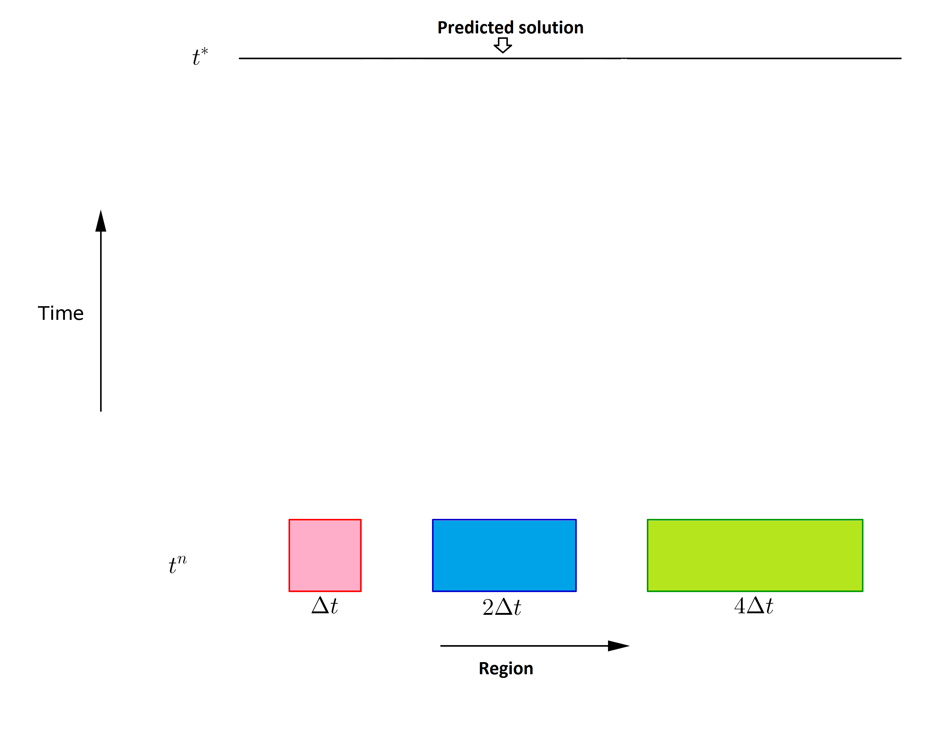
(a)

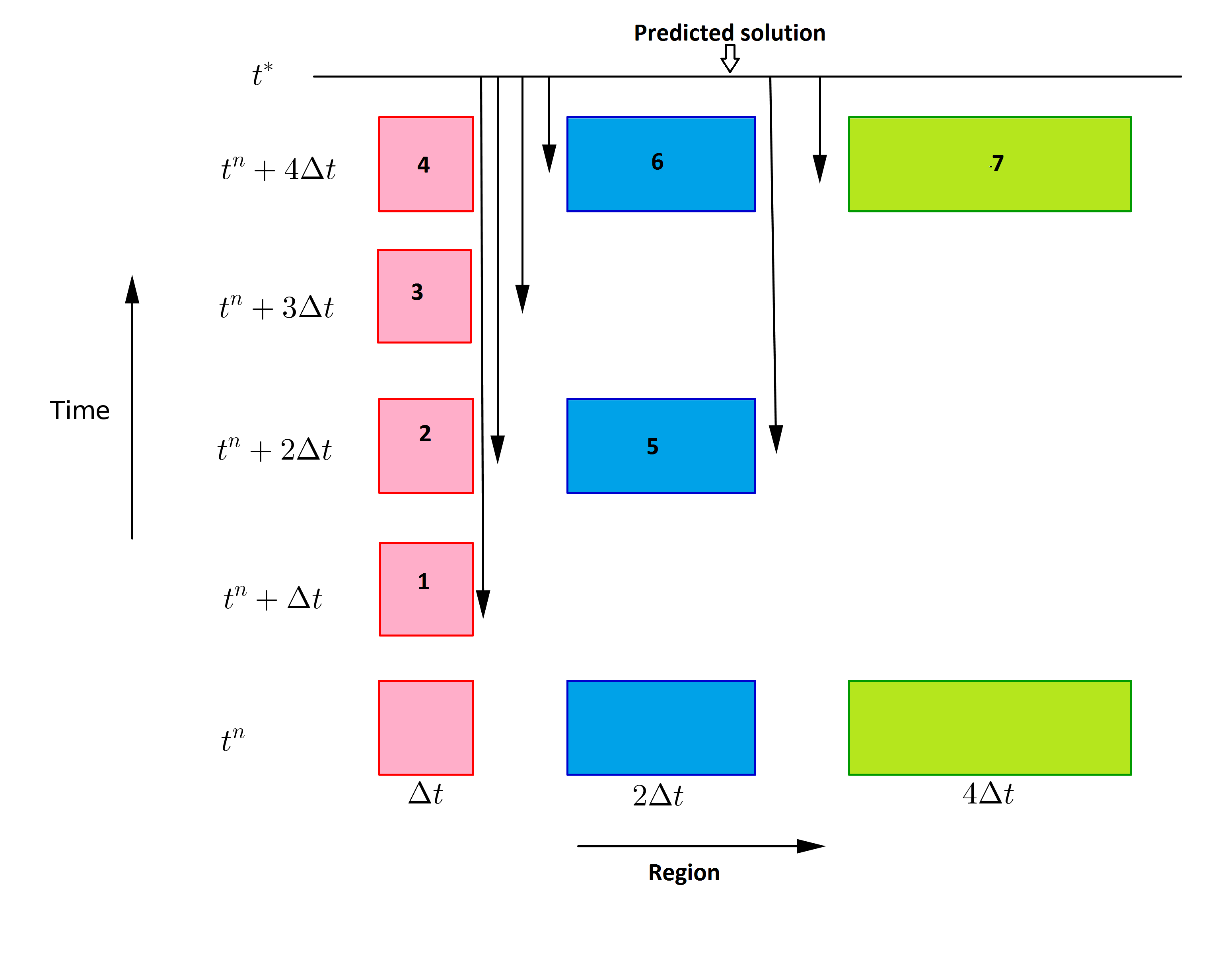
(b)

Figure 6: (a) Prediction step and (b) correction step of the non overlap LTS method, when domain $\Omega$ is split into three regions $\Omega_{0},\Omega_{1}$ and $\Omega_{2}$ respectively with time step $\Delta t,2\Delta t$ and $4\Delta t$.

This process can be repeated, in order to estimate the solution at any final time $T^{1}$ from the known solution at initial time $T^{0}$. To that end, one can implement Algorithm 2 with $m_{s}=\frac{T^{1}-T^{0}}{\Delta t_{\max}}$ and $r_{i}=\frac{\Delta t_{\max}}{\Delta t_{i}}$ for all $i\in\{0,\cdots,m\}$. Here, the function $\mathbf{I}$ is the interpolation function while the functions $\mathbf{A}_{G}$ and $\mathbf{A}_{i}$ are the iterative function of the standard time integrators respectively used to solve the system of ODEs globally on $\Omega$ and locally on $\Omega_{i}$.

Algorithm 2 Pseudo algorithm of the non overlap LTS method.

for $i=0\text{ to }m-1$ do

     $r_{i}=\frac{\Delta t_{\max}}{\Delta t_{i}}$$\triangleright$ Number of steps needed to advance locally $X_{i}$ to a synchronized time using time step $\Delta t_{i}$

end for

for $n=0\text{ to }m^{s}-1$  do$\triangleright$ Loop to advance the solution from $T^{0}$ to $T^{1}$

     $t^{n}=T^{0}+n\times\Delta t_{\max}$$\triangleright$ Compute the synchronized time $t^{n}$

     $t^{*}=t^{n}+\Delta t^{*}$$\triangleright$ Compute the prediction time $t^{*}$

     $X\Bigr{|}_{t^{*}}=\mathbf{A}_{G}\left(X\Bigr{|}_{t^{n}}\right)$$\triangleright$ Computation of predicted global solution at time $t^{*}$

     for $i=0\text{ to }m-1$ do$\triangleright$ Loop over all local regions - Correction step

         $t^{old}_{i}=t^{n}$$\triangleright$ initialize the time of the known local solution $X_{i}$

         for $j=1\text{ to }r_{i}$  do$\triangleright$ Loop to advance the solution from $t^{n}$ to $t^{n+1}$ locally on $\Omega_{i}$

              $t^{j}_{i}=t^{old}_{i}+\Delta t_{i}$$\triangleright$ Compute the local advancing time $t^{j}_{i}$

              $X\Bigr{|}_{\Gamma_{i},t^{j}_{i}}=\mathbf{I}\left(X\Bigr{|}_{t^{*}},X\Bigr{|}_{t^{n}}\right)$$\triangleright$ Interpolate the local solution $X_{i}$ on the boundary $\Gamma_{i}$ at time $t_{new}^{i}$

              $X_{i}\Bigr{|}_{t^{j}_{i}}=\mathbf{A}_{i}\left(X_{i}\Bigr{|}_{t^{old}_{i}},X\Bigr{|}_{\Gamma_{i},t^{j}_{i}}\right)$$\triangleright$ Advance locally the solution on $\Omega_{i}$ from $t^{old}_{i}$ to $t^{j}_{i}$

              $t^{old}_{i}=t_{i}^{j}$$\triangleright$ Update the time of the known local solution $X_{i}$

         end for

     end for

end for

3 Results and Discussion

The goal of this section is to investigate numerically the convergence of LTS-DG schemes and compare their efficiency against a global time stepping (GTS-DG) scheme. Firstly in Subsection 3.1, by applying the OLTS-DG scheme to the two dimensional Ogata and Banks problem [46], we examine how the direction of the bulk velocity of the DAREs and the size of the overlap affect the accuracy of the OLTS-DG schemes. Secondly in Subsection 3.2, we compare the efficiency of the GTS-DG, OLTS-DG and NOLTS-DG schemes, by applying them to the one dimensional electron transfer only (ETO) model [9]. Finally, in Subsection 3.3, we examine the convergence and compare the efficiency of the GTS-DG and OLTS-DG when applied to the transport of solute through a 2D domain with fracture.

3.1 Effect of the bulk velocity and the size of overlap on the OLTS-DG schemes

The purpose of this section is to investigate how the direction of the bulk velocity or the size of the overlap and the order in which the solution restraints to the eligible sub-domains $S^{r}$ are consecutively solved, affect the accuracy of the numerical solution obtained with OLTS-DG schemes. To that end, the $DG_{\text{OLTSD-Impl}}$ and $DG_{\text{OLTSI-Impl}}$ schemes are used to solve the Ogata Banks equation with the bulk velocity $\beta=(1,0)$ and the diffusion coefficient $\epsilon=\frac{\parallel\beta\parallel}{Pe}$ where $Pe$ is the Péclet number.

3.1.1 Effect of the bulk velocity on the OLTS-DG schemes

In the Ogata and Banks problem [46], the fast change of the concentration of the solute takes place in a region close to the boundary at $x=0$. So the sub-domain that contains the boundary at $x=0$ should have the finest local time step, for a high accuracy of the OLTS-DG methods. This is illustrated by the better accuracy of both OLTS-DG methods obtained in the case where the sub-domain containing the boundary $x=0$ has the finest time step compared to case where it has the coarser time step (see [41] for more details). Thus, to improve the efficiency of the OLTS-DG method, the choice of the fine, coarse discretized sub-domains and the order of update of the local solution should respect the a priori physics.

3.1.2 Effect of the size of overlap on the OLTS-DG schemes

In this section, we investigate how the size of the overlap between two sub-domains affect the accuracy of the global solution. To that end, we consider the Ogata and Banks problem [46] with the initial sub-domains $\Omega_{0}=[0,x_{1}]\times[0,1]$ and $\Omega_{1}=[x_{1},x_{2}]\times[0,1]$. For a given $n\in\{1,2,\cdots,11\}$ and $h_{x}=0.02$, we consider the overlapped sub-domains $\Omega_{0,n}$ and $\Omega_{1,n}$ given by

$$\Omega_{0,n}=[0,x_{1}+n\times h_{x}]\times[0,1],\qquad\Omega_{1,n}=[x_{1}-n\times h_{x},x_{2}]\times[0,1].$$ (11)

Note that the size of the overlap (i.e. $(\Omega_{0,n}\bigcap\Omega_{1,n}$) is equal to $2n\times h_{x}$ and increases with $n$. The local time steps are $\Delta t_{0}=2^{-11}$ and $\Delta t_{1}=2^{-10}$, thus we consider the $DG_{\text{OLTSI-Impl}}$ scheme for more accuracy.

For all Péclet number $P_{e}\in\{0.1,1,10,100\}$ and all $n\in\{1,2,\cdots,11\}$, we simulate the global solution, $C_{P_{e}}^{n}$ at the time $t=0.5$, using the $DG_{\text{OLTSI-Impl}}$ scheme on the overlapped sub-domains $(\Omega_{0,n},\;\Delta t_{0})$ and $(\Omega_{1,n},\;\Delta t_{1})$. We then compute the relative error $E_{P_{e}}^{n}$ as follows

$$E_{P_{e}}^{n}=\frac{\Bigr{|}C_{P_{e}}^{n}-C\Bigr{|}_{L^{2}(\Omega)}}{\Bigr{|}C\Bigr{|}_{L^{2}(\Omega)}},$$ (12)

where $C$ is the exact solution at the time $t=0.5$ and $\Omega$ the solution domain. The results are illustrated in Figure 7, where we plot the logarithm relative error ($\log(E_{P_{e}}^{n})$) against the integer $n$ for all the Péclet numbers considered. A few conclusions can be drawn from the results Figure 7:

• For the Péclet number $P_{e}>1$ ($\epsilon<1$), the relative error $E_{P_{e}}^{n}$ increases slightly as we increase the size of the overlap (i.e. as we increase $n$). Thus, in the case of high Péclet number, the overlapped sub-domains obtained by including only the direct neighbour into the initial sub-domains, is the best choice to simulate efficiently the global solution.

• For the Péclet number $P_{e}\leq 1$ ($\epsilon\geq 1$), the relative error $E_{P_{e}}^{n}$ decreases as we increase the size of the overlap (i.e $n$).

• For large size of overlap, i.e. $n>>1$, the relative error $E_{P_{e}}^{n}$ decreases as we decrease the Péclet number $P_{e}$ (or increase $\epsilon$). The same behaviour is observed in [36], when the overlapping Schwarz waveform relaxation scheme was applied to the viscous Burger equation with various values of the viscosity parameter. For the overlap equal $0.2$ ($n=10$ in our case), the error decreases as the diffusion term increases.

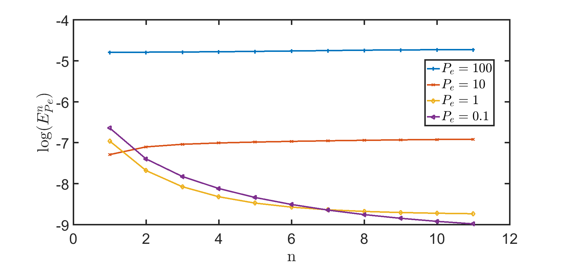
Figure 7: We plot the logarithm relative error ($\log(E_{P_{e}}^{n})$) against the integer $n$ for all Péclet number considered. The size of the overlap is equal to $2n\times h_{x}$ with $h_{x}=0.02$

3.2 Comparison of GTS-DG and LTS-DG schemes when applied to the 1D ETO model

In this section, we compare the performance of the GTS-DG and LTS-DG schemes, when solving the one dimension ETO model. To that end, we first describe how we split the global solution domain. Secondly, we investigate the derivation of the local system $\text{SO}_{i}$ associated to the sub-domain $\Omega_{i}$ for all $i=0,\cdots,m$. Finally, we present the numerical results. Here, we consider the LTS-DG schemes that use the Impl as time integrator. Thus we respectively denote $DG_{\text{OLTS-Impl}}$ and $DG_{\text{NOLTS-Impl}}$ the overlap and non overlap LTS-DG schemes.

Let us consider for example the ETO process at the electrode represents by the chemical reaction defined as follow

$$\mathbf{Q}\xrightleftharpoons[k_{b}]{k_{f}}\mathbf{Q}^{+}+e^{-},$$ (13)

where the rate constants $k_{b}$ and $k_{f}$ are given by the Buttle-Volmer kinetics Equation [9]. The mathematical model to describe ETO is derived from the Fick’s Law for mass transfer [11, 35, 34]. In one dimension, the dimensionless governing equation of ETO model is a coupled system of PDEs given by

$$\partial_{t}C_{\mathbf{Q}}= \partial_{z}(\partial_{z}C_{\mathbf{Q}}),\;\; \forall(t,z)\in[0,2t_{\lambda}]\times[0,z_{\max}],$$ (14a)

$$\partial_{t}C_{\mathbf{Q}^{+}}= \partial_{z}(D^{+}\partial_{z}C_{\mathbf{Q}^{+}}),\;\; \forall(t,z)\in[0,2t_{\lambda}]\times[0,z_{\max}],$$ (14b)

subject to the boundary conditions

$$\partial_{z}C_{i}(t,z_{\max})= 0,\;\;\forall t\in[0,2t_{\lambda}],\;\;\forall i\in\{\mathbf{Q},\mathbf{Q}^{+}\},$$ (15a)

$$\partial_{z}C_{\mathbf{Q}}(t,0)= K_{f}(t)C_{\mathbf{Q}}(t,0)-K_{b}(t)C_{\mathbf{Q}^{+}}(t,0),\;\;\forall t\in[0,2t_{\lambda}],$$ (15b)

$$D^{+}\partial_{z}C_{\mathbf{Q}^{+}}(t,0)= -K_{f}(t)C_{\mathbf{Q}}(t,0)+K_{b}(t)C_{\mathbf{Q}^{+}}(t,0),\;\;\forall t\in[0,2t_{\lambda}],$$ (15c)

and the initial condition

$$C_{\mathbf{Q}}(0,z)=1,\;\;C_{\mathbf{Q}^{+}}(0,z)=0,\;\;\forall z\in[0,z_{\max}].$$ (16)

Here $C_{i}(t,z)\in\mathbb{R}$ is the dimensionless concentration of the species $i\in\{\mathbf{Q},\mathbf{Q}^{+}\}$ and $D^{+}\in\mathbb{R}$ is the dimensionless diffusion of the specie $\mathbf{Q}^{+}$. The heterogeneous electron transfer rate constants, $k_{b},k_{f}$, can be written in its dimensionless form, $K_{b},K_{f}$, as follows

$$K_{f}=K_{0}\exp[(1-\delta)P],\qquad K_{b}=K_{0}\exp[(-\delta)P],$$ (17)

where the dimensionless potential, $P$, in terms of the dimensionless time, is given by

$$P=\left\{\begin{array}[]{ll}P_{1}+t,\;0\leq t\leq t_{\lambda}\\ P_{2}-(t-t_{\lambda}),\;t_{\lambda}\leq t\leq 2t_{\lambda}\end{array}\right.,\qquad t_{\lambda}=P_{2}-P_{1},$$ (20)

with $P_{1}$ and $P_{2}$ respectively the dimensionless initial and reverse potential. The dimensionless current, $G$, is given by

$$G(t)=\partial_{z}C_{\mathbf{Q}}(t,0)=K_{f}(t)C_{\mathbf{Q}}(t,0)-K_{b}(t)C_{\mathbf{Q}^{+}}(t,0),\;\;\forall t\in[0,2t_{\lambda}].$$ (21)

The solution domain is given by $\Omega=[0,z_{\max}]$, with $z_{\max}$ proportional to the diffusion length $\delta$ (i.e. $z_{\max}=k\delta,\;k\in\mathbb{N})$. Since the dimensionless current depends only on the concentration of the species at the boundary $z=0$, we consider the partition $\Omega=\cup_{i=1}^{n}I_{i}$ where the interval $I_{i}=[z_{i-1},z_{i}]$ is such that the step size $h_{i}=z_{i}-z_{i-1}$, respectively, follows the geometric and the uniform progression on $[0,\delta]$ and $[\delta,z_{max}]$. Specifically for a given number $r\in\mathbb{N}$ and the increasing factor $q$, we have

$$h_{i}=\left\{\begin{array}[]{ll}h\times q^{i-1},&i=1,\cdots,r\\ h\times q^{r},&i=r+1,\cdots,n\end{array}\right.,h=\delta\left(\frac{q^{r}-1}{q-1}\right)^{-1},n=r+\lceil\frac{z_{\max}-\delta}{h_{r}}\rceil.$$

Unless stated, for the simulation we use $q=1.05$ and $r=100$. We associate to each element $I_{i}$ the time step $\Delta T_{I_{i}}\leq 2^{n_{i}},\;n_{i}=\lceil\log_{2}\left(\mathbf{C}_{max}h_{i}\right)\rceil$ for a given Courant number $\mathbf{C}_{max}$. We then update the time step on each element $I_{i}$ by setting $\Delta T_{I_{i}}=\Delta T_{I_{1}}$ for all $i=1,\cdots,r$ and $\Delta T_{I_{i}}=\Delta T_{I_{r+1}}$ for all $i=r+1,\cdots,n$.

For the simulation, we consider the geometry settings and the ETO model parameters given by

$$\delta=20,z_{\max}=5\delta,\mathbf{C}_{max}=0.3,K_{0}=20,\tilde{D}^{+}=1.$$ (22)

This leads to the local time steps $\Delta t_{I_{1}}\leq 2^{-9}$ and $\Delta t_{I_{r+1}}\leq 2^{-2}$. We finally consider the sub-domains $\Omega_{0}=[0,z_{r}]$ and $\Omega_{1}=[z_{r},z_{n}]$ with the local time step $\Delta t_{0}=2^{-9}$ and $\Delta t_{1}=2^{-6}$, respectively.

By considering an orthonormal DG finite space, the DG space discretization of the governing equation of the ETO model leads to the system of ODEs defined as follows

$$\underbrace{\left(\begin{array}[]{c}d_{t}\alpha\\ d_{t}\alpha^{+}\end{array}\right)}_{d_{t}\chi}+\underbrace{\left(\begin{array}[]{cc}L^{s,\sigma_{0}}+K_{f}(\tilde{t})F^{1}&-K_{b}(\tilde{t})F^{1}\\ -K_{f}(\tilde{t})F^{1}&D^{+}L^{s,\sigma_{0}}+K_{b}(\tilde{t})F^{1}\end{array}\right)}_{\mathcal{L}^{s,\sigma_{0}}_{D^{+},K_{f},K_{b}}}\underbrace{\left(\begin{array}[]{c}\alpha\\ \alpha^{+}\end{array}\right)}_{\chi}=\left(\begin{array}[]{c}0\\ 0\end{array}\right).$$ (23)

Here $\alpha$ and $\alpha^{+}$ are respectively the components of the concentration of the species $Q$ and $Q^{+}$ in the DG finite space. The matrix $L^{s,\sigma_{0}}$ represents the DG driscretization of the diffusion operator. More details on this derivation can be found in [41].

3.2.1 Local ODE system for the overlap LTS-DG scheme

In this section, we show how to extract the local ODE system for the OLTS-DG scheme from the global ODE system of the 1D ETO model. To overlap the sub-domains here, we include the direct neighbour into the initial sub-domains. Thus, the overlapped sub-domains are $\Omega_{0}=[0,z_{r+1}]$ and $\Omega_{1}=[z_{r-1},z_{n}]$. In this case, we consider as internal boundary $\Gamma_{0}$ and $\Gamma_{1}$ as the node $z_{r+1}$ of $[z_{r+1},z_{r+2}]$ and $z_{r-1}$ of $[z_{r-2},z_{r-1}]$, respectively. The system of ODEs given by Equation 23, obtained from the DG spatial discretization of the dimensionless governing equation of the ETO model, can be split into two systems of ODEs

$$\dfrac{d\chi_{0}}{d\tilde{t}}=L_{0}(\tilde{t})\chi_{0}+\mathbb{S}_{0}^{e}\chi_{1}\Bigr{|}_{\Gamma_{0}},$$ (24)

$$\dfrac{d\chi_{1}}{d\tilde{t}}=L_{1}(\tilde{t})\chi_{1}+\mathbb{S}_{1}^{e}\chi_{0}\Bigr{|}_{\Gamma_{1}},$$ (25)

where $\chi_{j}\in\mathbb{R}^{2n_{\Omega_{j}}}$ is the coupled component of the concentration of the species $\mathbf{Q},\mathbf{Q}^{+}$ on the region $\Omega_{j}$ for all $j=0,1$. The dimensions $n_{\Omega_{0}}$ and $n_{\Omega_{1}}$ are given by

$$n_{\Omega_{0}}=\sum_{i=1}^{r+1}(k_{i}+1),\qquad n_{\Omega_{1}}=\sum_{i=r}^{n}(k_{i}+1),$$ (26)

where $k_{i}$ is the highest degree of the Legendre polynomials considered on $I_{i}$ (i.e. $k_{i}+1$ is the dimension of the DG finite space on $I_{i}$). The matrices $L_{j},\mathbb{S}_{j}^{e}\in\mathbb{R}^{2n_{\Omega_{j}}\times 2n_{\Omega_{j}}}$ for all $j=0,1$ can be obtained from the matrix $\mathcal{L}^{s,\sigma_{0}}_{D^{+},K_{f},K_{b}}$, given by Equation 23, as follows

$$L_{1}=\left(\begin{array}[]{c|c}DL_{0,0}^{s,\sigma_{0}}+K_{f}(\tilde{t})L^{1}&-K_{b}(\tilde{t})L^{1}\\ \hline\cr-K_{f}(\tilde{t})L^{1}&D^{+}L_{0,0}^{s,\sigma_{0}}+K_{b}(\tilde{t})L^{1}\end{array}\right),\;L_{2}=\left(\begin{array}[]{c|c}DL_{0,1}^{s,\sigma_{0}}&0\\ \hline\cr 0&D^{+}L_{0,1}^{s,\sigma_{0}}\end{array}\right).$$ (27)

Here, the matrix $L^{1}\in\mathbb{R}^{n_{\Omega_{0}}\times n_{\Omega_{0}}}$ takes the same form as the matrix $F^{1}$ defined in Equation 23; the matrices $L_{0,0}^{s,\sigma_{0}}$ and $L_{0,1}^{s,\sigma_{0}}$ are efficiently extracted from the matrix $L_{0}^{s,\sigma_{0}}$ as illustrated by Figure 8, due to its tridiagonalisation. Note from Figure 8 that only the block matrices $L_{0,I_{r+2}I_{r+1}}^{s,\sigma}$ and $L_{0,I_{r-1}I_{r}}^{s,\sigma}$, from the matrix $L_{0}^{s,\sigma_{0}}$ respectively contribute to the computation of the vector $\mathbf{B}_{0}^{T}=\mathbb{S}_{0}^{e}\chi_{1}\Bigr{|}_{\Gamma_{0}}$ and $\mathbf{B}_{1}^{T}=\mathbb{S}_{1}^{e}\chi_{0}\Bigr{|}_{\Gamma_{1}}$.

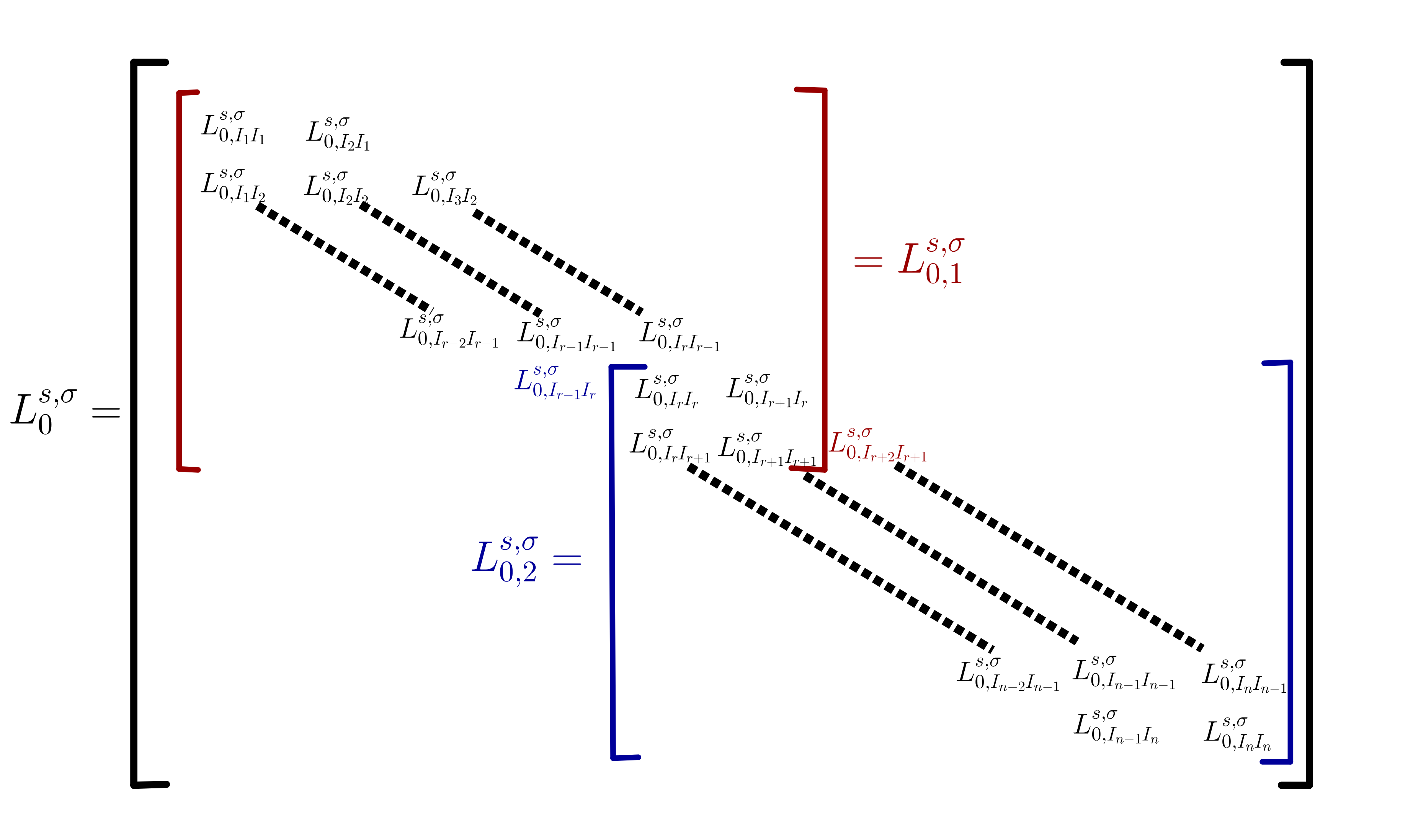
Figure 8: Extraction of the matrices $L_{0,1}^{s,\sigma_{0}}$ and $L_{0,1}^{s,\sigma_{0}}$ from the stiffness matrix $L_{0}^{s,\sigma_{0}}$ when applying the overlap LTS method to the one dimension ETO model. It shows that only the block matrices $L_{0,I_{r+2}I_{r+1}}^{s,\sigma}$ and $L_{0,I_{r-1}I_{r}}^{s,\sigma}$, from the matrix $L_{0}^{s,\sigma_{0}}$ respectively contribute to the computation of the vectors $\mathbf{B}_{1}^{T}$ and $\mathbf{B}_{2}^{T}$.

For all $j\in\{0,1\}$, we have $\mathbf{B}_{j}=[\mathbf{B}_{j}^{\alpha},\mathbf{B}_{j}^{\alpha^{+}}]$ where the transpose of the block vectors $\mathbf{B}_{j}^{\alpha},\mathbf{B}_{j}^{\alpha^{+}}\in\mathbb{R}^{1\times n_{\Omega_{j}}}$ are given by

$$\mathbf{B}_{0}^{\zeta}=\left(\mathbf{B}_{0,I_{i}}^{\zeta}\right)_{i=1,\cdots,r+1},\quad\mathbf{B}_{1}^{\zeta}=\left(\mathbf{B}_{1,I_{p_{i}}}^{\zeta}\right)_{i=1,\cdots,n-r+1},\;p_{i}=i+r-1,$$ (28)

for all $\zeta=\alpha,\alpha^{+}$. According to the extraction of matrices illustrated in Figure 8, we have for all $\zeta=\alpha,\alpha^{+}$

$$\mathbf{B}_{0,I_{i}}^{\zeta}= \left\{\begin{array}[]{ll}D^{\zeta}L_{0,I_{r+2}I_{r+1}}^{s,\sigma}\zeta_{I_{r+2}}&\text{if}\;\;i=r+1\\ 0&\text{if}\;\;i=1,\cdots,r\end{array}\right.,$$

$$\mathbf{B}_{1,I_{p_{i}}}^{\zeta}= \left\{\begin{array}[]{ll}D^{\zeta}L_{0,I_{r-1}I_{r}}^{s,\sigma}\zeta_{I_{r-1}}&\text{if}\;\;i=1\\ 0&\text{if}\;\;i=2,\cdots,n-r+2\end{array}\right.,$$

where the coefficient $D^{\zeta}$ is the dimensionless diffusion coefficient of the species with the component in the DG finite space $\zeta=\alpha,\alpha^{+}$.

3.2.2 Local ODE system for the non overlap LTS-DG scheme

In this section, we show how to extract the local ODE system for the NOLTS-DG scheme from the global ODE system of the 1D ETO model. The non overlapped sub-domains are $\Omega_{0}=[0,z_{r}]$ and $\Omega_{1}=[z_{r},z_{n}]$. In this case, we consider the node $z_{r}$ of the interval $[z_{r},z_{r+1}]$ and $[z_{r-1},z_{r}]$ as the internal boundary of $\Gamma_{0}$ and $\Gamma_{1}$ , respectively. The system of ODEs obtained from the DG spatial discretization of the dimensionless governing equation of the ETO model, can be split into two ODEs system of Equation 24 and Equation 25. In this case, the dimensions $n_{\Omega_{0}}$, $n_{\Omega_{1}}$ are given by

$$n_{\Omega_{0}}=\sum_{i=1}^{r}(k_{i}+1),\qquad n_{\Omega_{1}}=\sum_{i=r+1}^{n}(k_{i}+1),$$ (29)

where $k_{i}$ is the highest degree of the Legendre polynomials considered on $I_{i}$. Also, the matrices $L_{j},\mathbb{S}_{j}^{e}\in\mathbb{R}^{2n_{\Omega_{j}}\times 2n_{\Omega_{j}}}$ for all $j=0,1$ are given by Equation 27 where the matrix $L^{1}\in\mathbb{R}^{n_{\Omega_{0}}\times n_{\Omega_{0}}}$ takes the same form as the matrix $F^{1}$ defined in Equation 23; the matrices $L_{0,0}^{s,\sigma_{0}}$ and $L_{0,1}^{s,\sigma_{0}}$ are efficiently extracted from the matrix $L_{0}^{s,\sigma_{0}}$ as illustrated by Figure 9, due to its tridiagonalisation.

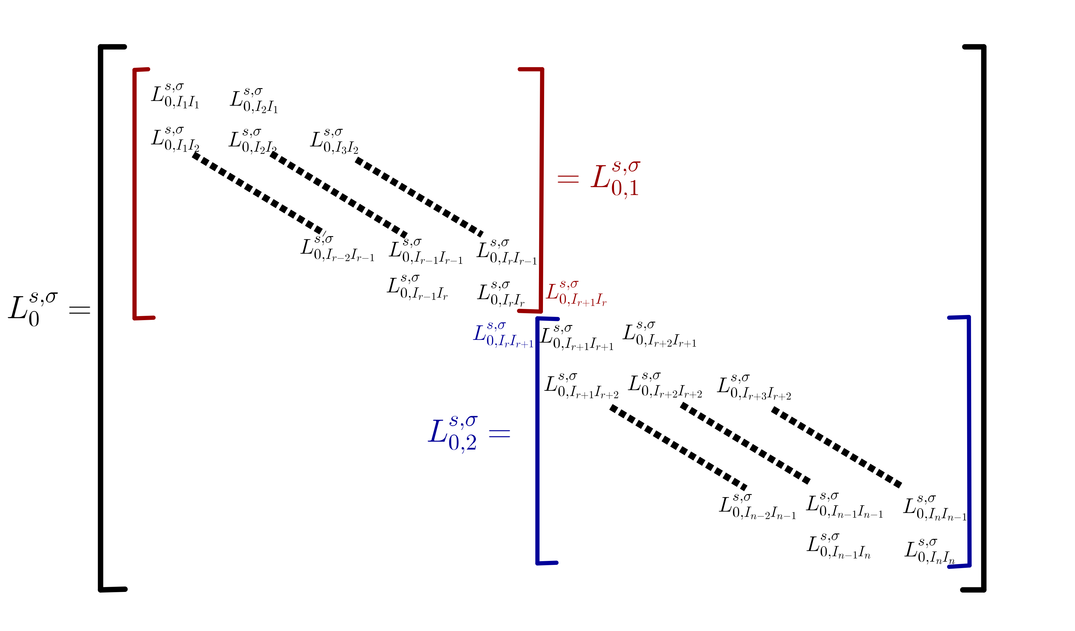
Figure 9: Extraction of the matrices $L_{0,1}^{s,\sigma_{0}}$ and $L_{0,1}^{s,\sigma_{0}}$ from the matrix $L_{0}^{s,\sigma_{0}}$ when applying the non overlap LTS method to the one dimension ETO model. It shows that only the block matrices $L_{0,I_{r+1}I_{r}}^{s,\sigma}$ and $L_{0,I_{r}I_{r+1}}^{s,\sigma}$, from the matrix $L_{0}^{s,\sigma_{0}}$ respectively contribute to the computation of the vectors $\mathbf{B}_{1}^{T}$ and $\mathbf{B}_{2}^{T}$.

Note from Figure 9 that only the block matrices $L_{0,I_{r+1}I_{r}}^{s,\sigma}$ and $L_{0,I_{r}I_{r+1}}^{s,\sigma}$, from the matrix $L_{0}^{s,\sigma_{0}}$ respectively contribute to the computation of the vector $\mathbf{B}_{0}^{T}=\mathbb{S}_{0}^{e}\chi_{1}\Bigr{|}_{\Gamma_{0}}$ and $\mathbf{B}_{1}^{T}=\mathbb{S}_{1}^{e}\chi_{0}\Bigr{|}_{\Gamma_{1}}$. For all $j\in\{0,1\}$, we have $\mathbf{B}_{j}=[\mathbf{B}_{j}^{\alpha},\mathbf{B}_{j}^{\alpha^{+}}]$ where the transposes of the block vectors $\mathbf{B}_{j}^{\alpha},\mathbf{B}_{j}^{\alpha^{+}}\in\mathbb{R}^{1\times n_{\Omega_{j}}}$ are given by

$$\mathbf{B}_{0}^{\zeta}=\left(\mathbf{B}_{0,I_{i}}^{\zeta}\right)_{i=1,\cdots,r},\quad\mathbf{B}_{1}^{\zeta}=\left(\mathbf{B}_{1,I_{p_{i}}}^{\zeta}\right)_{i=1,\cdots,n-r},\;p_{i}=i+r.$$ (30)

According to the extraction of matrices illustrated in Figure 9, we have for all $\zeta=\alpha,\alpha^{+}$,

$$\mathbf{B}_{0,I_{i}}^{\zeta}= \left\{\begin{array}[]{ll}D^{\zeta}L_{0,I_{r+1}I_{r}}^{s,\sigma}\zeta_{I_{r+1}}&\text{if}\;\;i=r\\ 0&\text{if}\;\;i=1,\cdots,r-1\end{array}\right.,$$

$$\mathbf{B}_{1,I_{p_{i}}}^{\zeta}= \left\{\begin{array}[]{ll}D^{\zeta}L_{0,I_{r}I_{r+1}}^{s,\sigma}\zeta_{I_{r}}&\text{if}\;\;i=1\\ 0&\text{if}\;\;i=2,\cdots,n-r+1\end{array}\right..$$

3.2.3 Numerical results of GTS-DG and LTS-DG schemes applied to the ETO model

Let us now focus on the numerical comparison of the accuracy and the efficiency of the GTS-DG and LTS-DG schemes, while simulating the dimensional current of the ETO model. To that end, for a given $i\in\{0,\cdots,4\}$, we simulate the dimensionless current $G^{i,q},$ $q=DG_{\text{Impl}}$, $DG_{\text{OLTS-Impl}}$, $DG_{\text{NOLTS-Impl}}$ for the local time step $\Delta t_{j}^{i}=2^{-i}\times\Delta t_{j}$ on the local solution domain $\Omega_{j}$ for all $j=0,1$. Note that for a given $i\in\{0,\cdots,4\}$, the universal time step, $ht^{i}=\Delta t_{0}^{i}$ , is considered for the GTS-DG schemes (i.e. the finest local time step of LTS-DG schemes). During the simulation of $G^{i,q}$, we also record the computation time $\text{CPU}^{i,q}$.

By assuming that the exact dimensionless current is given by $G^{4,DG_{\text{Impl}}}$, we then compare it against $G^{4,q}$ $q=DG_{\text{OLTS-Impl}}$, $DG_{\text{NOLTS-Impl}}$ to see which of the LTS-DG schemes is more accurate. This is illustrated in Figure 10, by plotting the dimensionless currents $G^{4,q}$ against the overpotential for all $q=DG_{\text{Impl}}$, $DG_{\text{OLTS-Impl}}$, $DG_{\text{NOLTS-Impl}}$ in Figure 10(a); and the absolute difference $E_{\text{abs}}^{q}=\Bigr{|}G^{4,DG_{\text{Impl}}}-G^{4,q}\Bigr{|}$ against the overpotential for all $q=DG_{\text{OLTS-Impl}},DG_{\text{NOLTS-Impl}}$ in Figure 10(b).

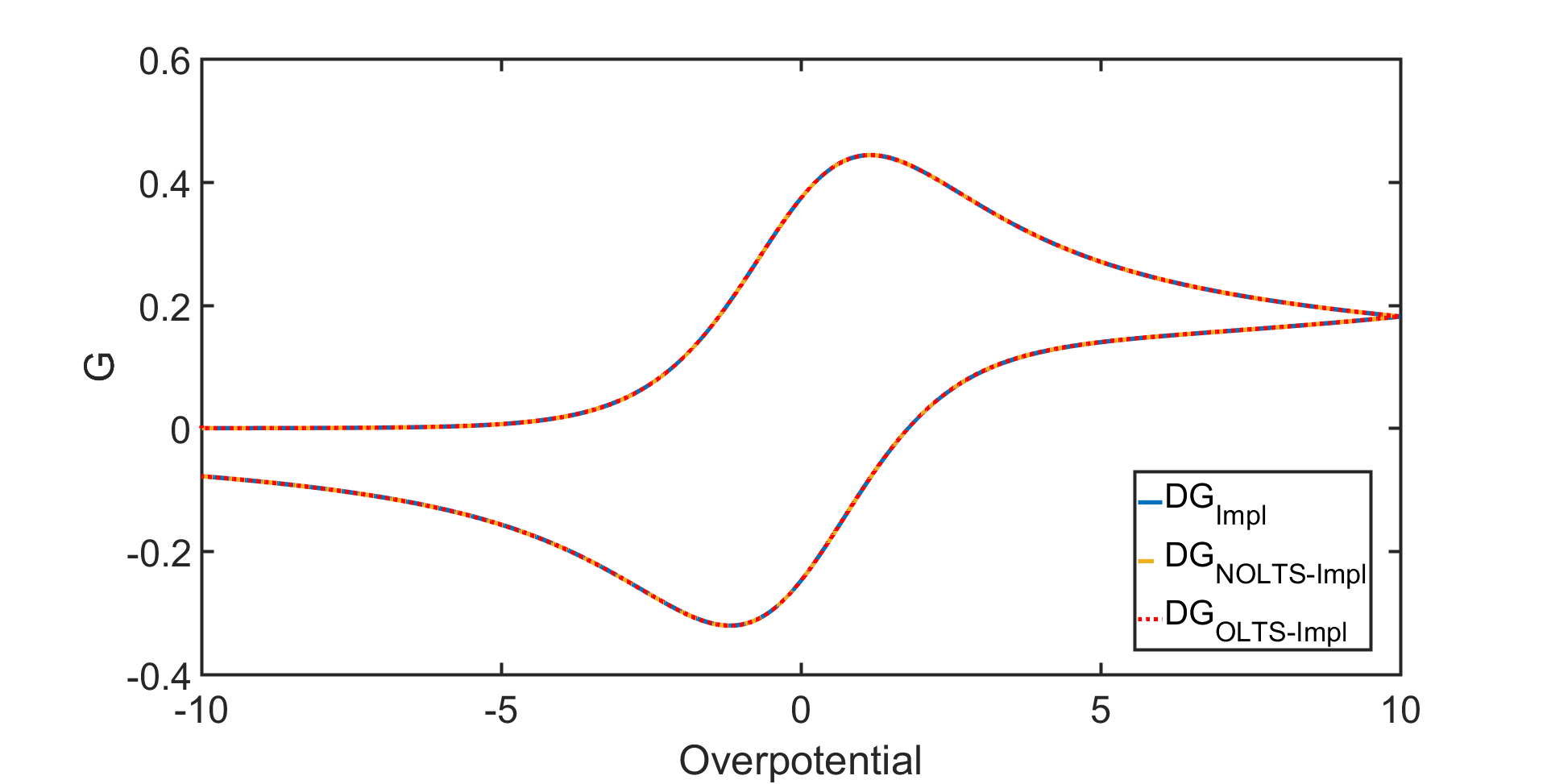
(a)

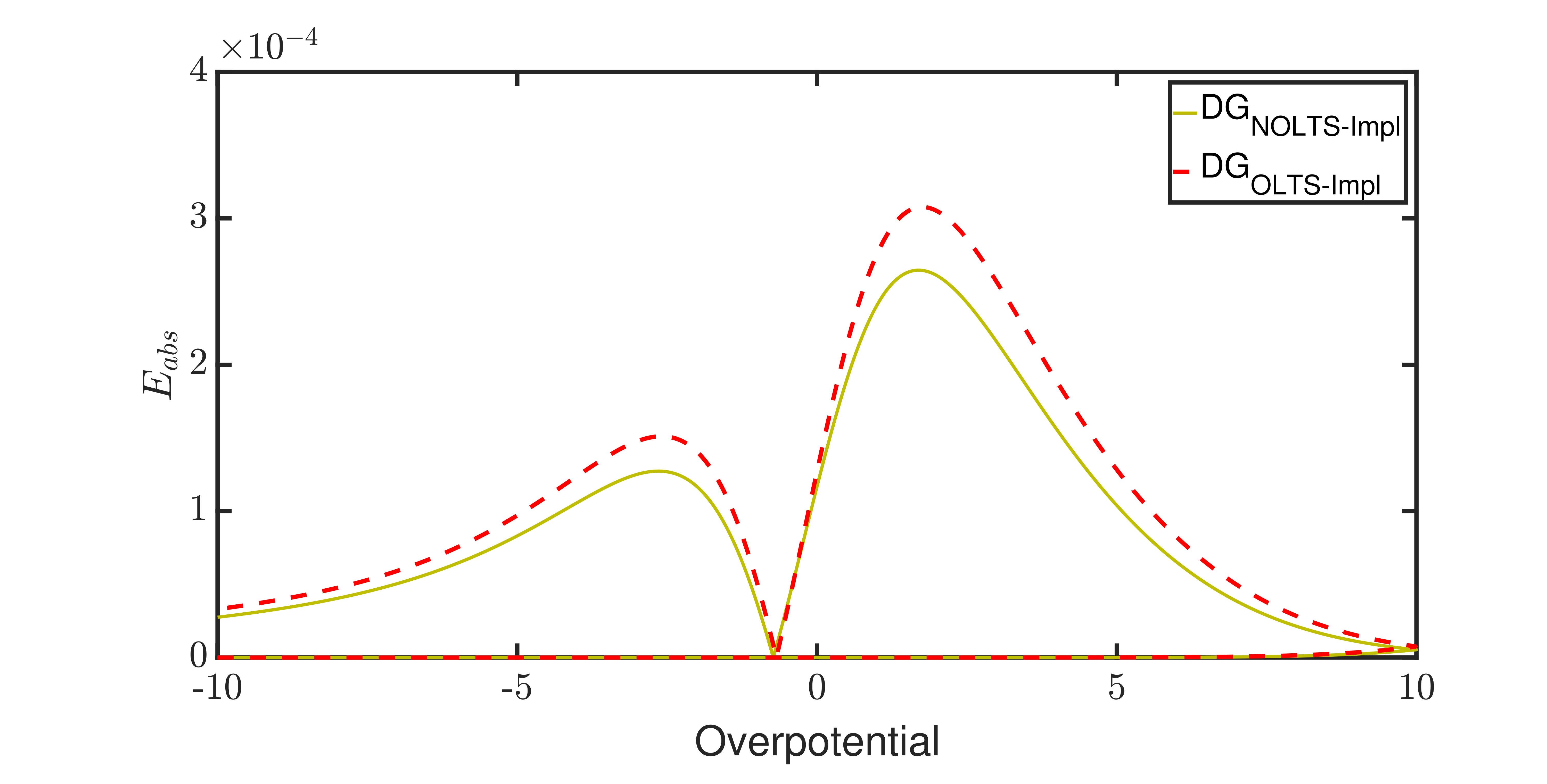
(b)

Figure 10: Voltammogram of the ETO model simulate with GTS-DG and LTS-DG schemes. In (a), we plot $G^{0,q}$ against the overpotential for all $q=DG_{\text{Impl}},DG_{\text{OLTS-Impl}},,DG_{\text{NOLTS-Impl}}$. In (b), we plot the absolute difference $E_{\text{abs}}^{q}$ against the overpotential for all $q=DG_{\text{OLTS-Impl}},,DG_{\text{NOLTS-Impl}}$.

To investigate the convergence and the efficiency of the GTS-DG and LTS-DG schemes, we compute the relative errors, $\text{error}^{i}_{q}$ , given by

$$\text{error}^{i}_{q}=100\dfrac{\Bigr{|}G^{4,DG_{\text{Impl}}}-G^{i,q}\Bigr{|}_{L^{2}(P)}^{2}}{\Bigr{|}G^{4,DG_{\text{Impl}}}\Bigr{|}_{L^{2}(P)}^{2}},$$ (31)

for all $i=0,\cdots,3$ and all solver $q=DG_{\text{Impl}},DG_{\text{OLTS-Impl}},DG_{\text{NOLTS-Impl}}$. We then plot in Figure 11(a) the error , $\log(\text{error}^{i}_{q})$, against the minimum of the local time step, $\log(ht^{i})$. This shows the decay of the error with respect to the minimum local time step, meaning the $DG_{\text{Impl}}$, $DG_{\text{OLTS-Impl}}$, $DG_{\text{NOLTS-Impl}}$ converge in time. In Figure 11(b), we plot the error, $\log(\text{error}^{i}_{q})$, against the computation time, $\log(\text{CPU}^{i,q})$. Note from Figure 11(b) that for a given error $E\in\mathbb{R}$ such that $E=\text{error}^{i}_{q}$, $q=DG_{\text{Impl}},DG_{\text{OLTS-Impl}},DG_{\text{NOLTS-Impl}}$, we have

$$\text{CPU}^{i,DG_{\text{NOLTS-Impl}}}<\text{CPU}^{i,DG_{\text{OLTS-Impl}}}<\text{CPU}^{i,DG_{\text{Impl}}}.$$

Figure 11(b) shows that the LTS-DG schemes, compared to GTS-DG schemes, are more efficient to simulate the dimensionless current of the ETO model.

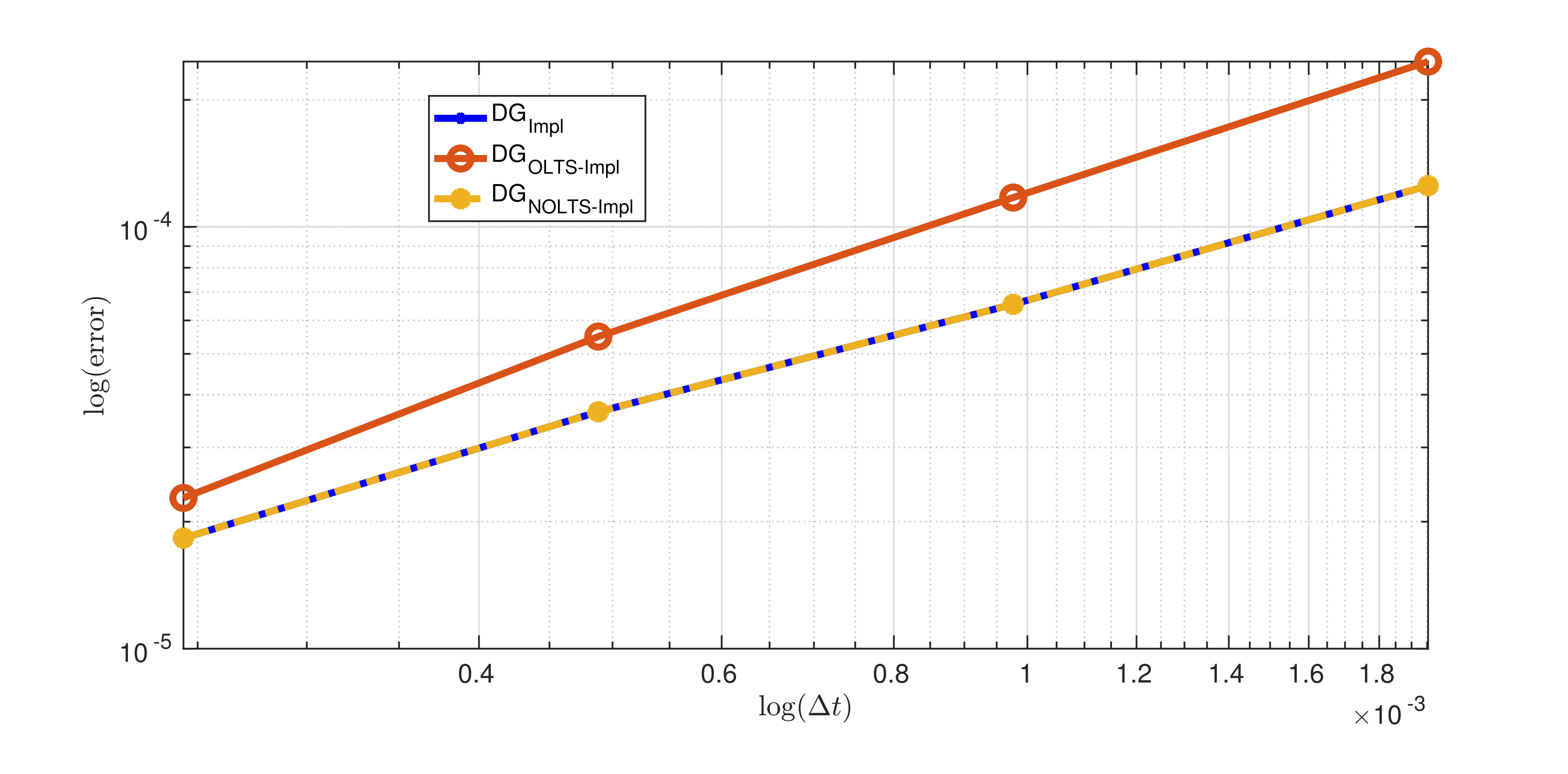
(a)

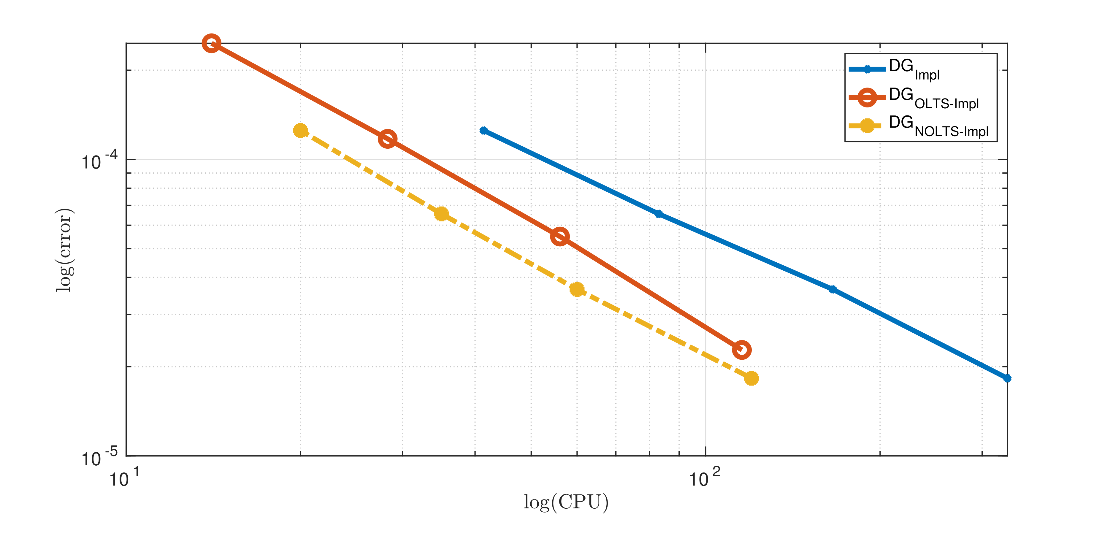
(b)

Figure 11: Convergence and efficiency of the GTS-DG and LTS-DG schemes for the ETO model. We plot in (a) the error $\log(\text{error}^{i}_{q})$ against the minimum time step $\log(ht^{i})$ and in (b) the computation time $\log(\text{CPU}^{i,q})$ for all $i=0,\cdots,3$ and all $q=DG_{\text{Impl}},DG_{\text{OLTS-Impl}},DG_{\text{NOLTS-Impl}}$.

The 1D numerical experiment realized in this section has shown that

• even if the OLTS-DG schemes is not as accurate as GTS-DG scheme, the computation time of the OLTS-DG schemes is small enough to make them more efficient compare to the GTS-DG schemes,

• the non overlap LTS-DG scheme is more accurate than the overlap LTS-DG scheme. This is because the estimation of the needed internal value $\Gamma_{i}$, for the resolution of the system $\text{SO}_{i}$, is more accurate with the non overlap LTS-DG scheme.

3.3 Comparison of GTS-DG and OLTS-DG schemes when applied to the 2D transport of solute through a domain with fracture

Consider the transport of an inert solute within an incompressible fluid with an absence of volumetric source and sinks, through a 2D domain, $\Omega$ with a fracture. The concentration $C(x,y,t)$ of the solute follows

$$\dfrac{\partial C}{\partial t}-\nabla\cdot(D_{m}\nabla C)+\nabla\cdot\textbf{v}C=R(C)\;\;\text{ with }\;\;R(C)=0,$$ (32)

where $R(C)$ is the reaction term, $D_{m}$ is a molecular diffusivity and the velocity v in each pore, computed from the solution of Darcy’s equation with the equation pressure given by

$$\textbf{v}=-\frac{\textbf{k}}{\mu\phi}\nabla p\;\;\text{ with }\;\;\left\{\begin{array}[]{lll}\nabla\cdot\left(-\frac{k}{\mu}\nabla p\right)&=0,&\\ p&=p_{0}&\text{in}\quad\partial\Omega_{D}^{1},\\ \vec{n}\cdot\left(-\frac{k}{\mu}\nabla p\right)&=p_{1}&\text{in}\quad\partial\Omega_{N}^{1}.\end{array}\right.$$ (33)

Here v is the fluid velocity, $p$ is the pressure, $\phi$ is the porosity, $k$ is the permeability, $\mu$ is the viscosity. As a boundary and initial condition, we keep the concentration $C$ and the pressure $p$ respectively at a constant value $C_{0}$ and $p_{0}$ at the inflow boundary $\partial\Omega_{2}$ and allow it to undergo pure advection at the outflow boundary $\partial\Omega_{4}$. The boundary conditions also include the no flux at the rigid boundaries, The fracture is represented by the domain $\Omega_{r}=[x_{r},x_{r}+l]\times[y_{r},y_{r}-h]$. We assumed that within the fracture, the permeability is 1000 times greater than the permeability of the remaining domain.

For the simulation of the concentration profile we design the unstructured mesh of the domain for $L=1$ with $distmesh2d$, such that for a given element $T$ within the fracture we have the radius on the incircle of $T$ is less than $h/3$. The finest elements are located in the fracture characterized by the coordinates $x_{r}=0.2,y_{r}=0.51$, the height $h=0.02$ and the length $l=0.6$. This is illustrated in Figure 1 (a).

In this case, the equation of the pressure is a steady heterogeneous diffusion equation given by Equation 33 with

$$p_{0}=1,\;p_{1}=0,\;k\mu^{-1}=\left\{\begin{array}[]{ll}1000&\quad\text{on}\quad\Omega_{r}\\ 1&\quad\text{on}\quad\Omega\setminus\Omega_{r}\end{array}\right..$$ (34)

We then simulate the fluid velocity on each element $T$ after using the SIPG method to solve the equation of the pressure. For the sake of clarity, we plot in Figure 12(a) the streamline of the simulated fluid velocity which shows, as expected, that the velocity of the fluid is higher within the fracture, thus the solute flows rapidly through the fracture see Figure 12(b).

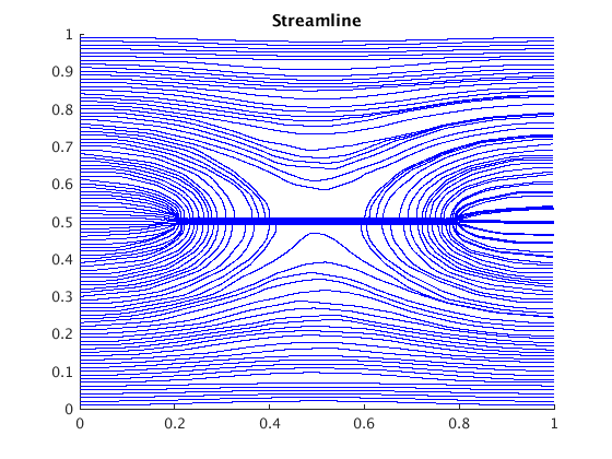
(a)

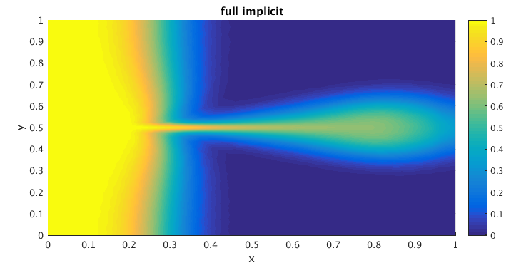
(b)

Figure 12: (a) Streamline of the simulated fluid velocity of solute through domain with fracture. Note from this figure that the velocity of the fluid is higher within the fracture. (b) Solution without presence of source or reaction ($R=0$) found using full implicit.

Once the vector field of the velocity is obtained, we compute the time step $\Delta t_{T}$ obtained using Equation 4 for $\mathbf{C}_{max}=0.08$. The solution domain $\Omega$ is split into sub-domain $(\Omega_{i},\Delta t_{i}),i=0,1,2$. Here, we consider the Péclet number $P_{e}=3000$. The overlapped sub-domains are illustrated in Figure 1 (b).

3.3.1 Numerical results for the case $R(C)=0$

For a given $r\in\{0,\cdots,4\}$, we simulate the concentration $C^{r}_{p}$ of the solute at the time $t=1$ using the solver $p\in\{DG_{\text{OLTS-Impl}},DG_{\text{OLTS-ETD1}}\}$ where the sub-domain $\Omega_{i}$ has the local time step $\Delta t^{r}_{i}=2^{-r}\times\Delta t_{i}$ for all $i\in\{0,1,2\}$. Moreover, for the GTS-DG schemes ($\{DG_{\text{Impl}}\}$) we use the universal time step $ht^{r}$ given by $ht^{r}=\min\{\Delta t^{r}_{i},\;i=0,1,2\},$ to simulate the concentration $C^{r}_{p}$, $r\in\{0,\cdots,4\}$ of the solute at the time $t=1$. Throughout these simulations (i.e. for all $r\in\{0,\cdots,4\}$), we record the computation time, $\text{CPU}^{r}_{p}$, for all solver $p\in\{DG_{Impl},DG_{\text{OLTS}-q}\}$. To investigate the convergence, the accuracy and efficiency of solvers used here, we assume that for a given time integrator $q\in\{Impl,ETD1\}$, the exact concentration of the solute at the time $t=1$ is given by $C^{4}_{DG_{q}}$. We then compute the error, $\text{error}^{r}_{p}$, given by

$$\text{error}^{r}_{DG_{q}}=\parallel C^{4}_{DG_{q}}-C^{r}_{DG_{q}}\parallel_{L^{2}(\mathcal{T})},\;\;\text{error}^{r}_{DG_{OLTS-q}}=\parallel C^{4}_{DG_{q}}-C^{r}_{DG_{OLTS-q}}\parallel_{L^{2}(\mathcal{T})},$$

for all $r\in\{0,\cdots,3\}$ and all time integrator $q\in\{Impl,ETD1\}$. In Figure 13(a), we plot the errors $\log(\text{error}^{r}_{DG_{Impl}})$ and $\log(\text{error}^{r}_{DG_{OLTS-q}})$ against $\log(ht^{r})$ for all $q=\text{Impl}$, ETD1 and $r=0,\cdots,3$. In Figure 13(b), we plot $\log(\text{error}^{r}_{DG_{q}})$ and $\log(\text{error}^{r}_{DG_{OLTS-q}})$ against $\log(\text{CPU}^{r}_{DG_{Impl}})$ and $\log(\text{CPU}^{r}_{DG_{OLTS-q}})$ for all $q=\text{Impl}$, ETD1 and $r=0,\cdots,3$. Note from Figure 13(a) that the errors $\text{error}^{r}_{p}$ decrease with the time step $ht^{r}$, meaning the GTS-DG and OLTS-DG schemes, considered in this section, converge. Also, note from Figure 13(a) that $\text{error}^{r}_{DG_{Impl}}<\text{error}^{r}_{DG_{OLTS-Impl}}.$ This shows that the OLTS-DG schemes is less accurate compared to GTS-DG schemes while using the same time integrator. This is expected since the GTS-DG schemes, unlike the OLTS-DG schemes, consider the finest time step, uniformly on the solution domain. However, note from Figure 13(b) that the computation time is reduced enough to make the OLTS-DG schemes more efficient compared to GTS-DG schemes. Moreover, Figure 13(a) shows that the accuracy improved with the accuracy of the time integrator, as $\text{error}^{r}_{DG_{OLTS-ETD1}}<\text{error}^{r}_{DG_{OLTS-Impl}}$ .

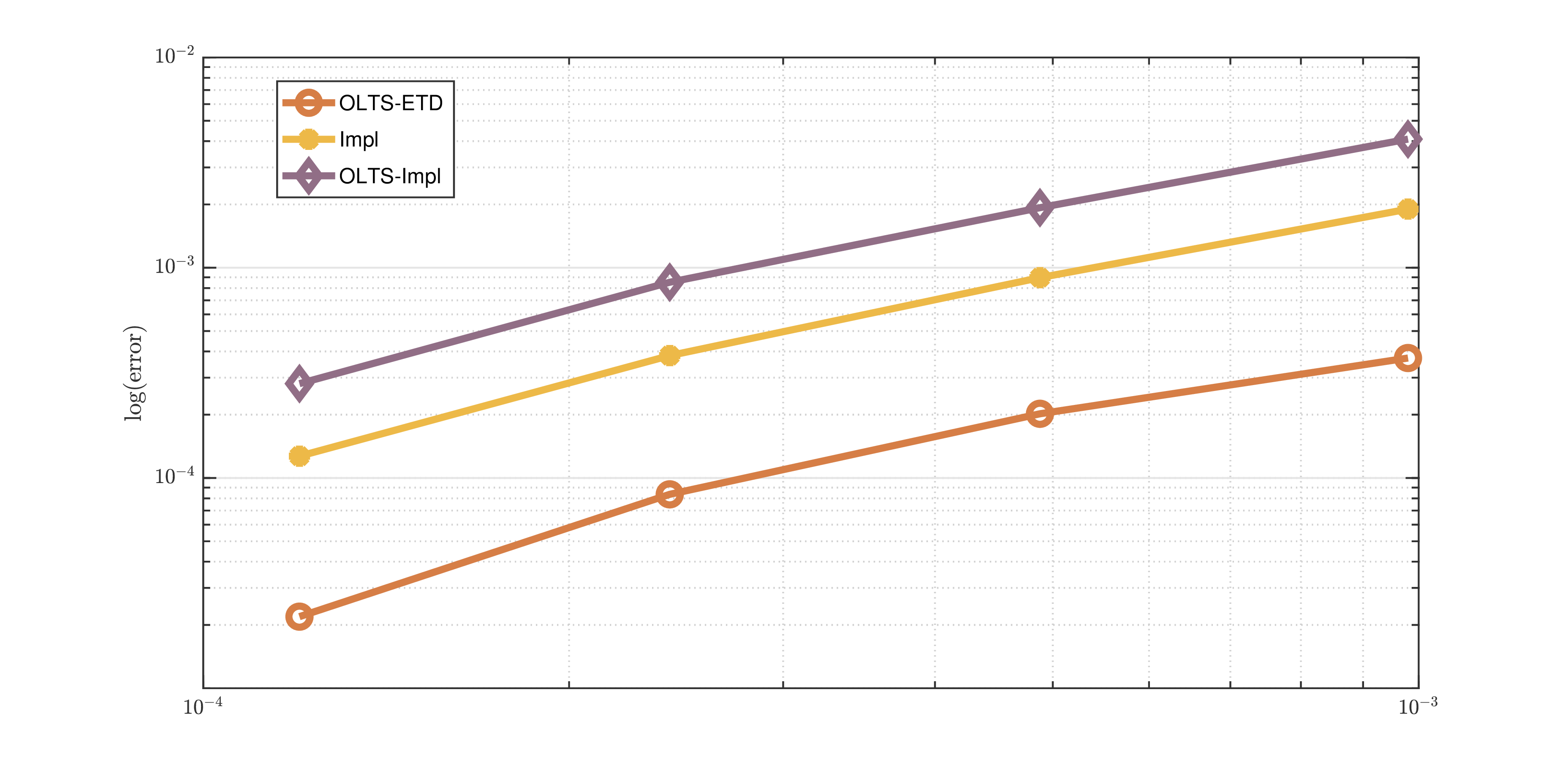
(a)

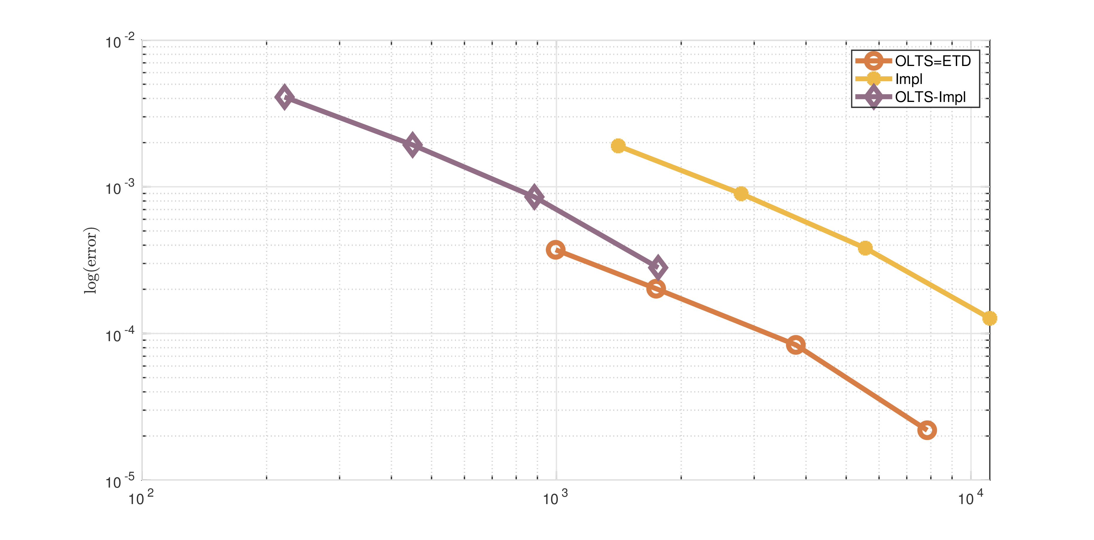
(b)

Figure 13: Convergence and efficiency of GTS-DG and OLTS-DG schemes while solving the transport of solute through a domain with fracture without presence of source and reaction. In (a), we plot $\log(\text{error}^{r}_{DG_{Impl}})$ and $\log(\text{error}^{r}_{DG_{OLTS-q}})$ against $\log(ht^{r})$ for all $q=\text{Impl}$, ETD1 and $r=0,\cdots,3$. In (b), we respectively plot $\log(\text{error}^{r}_{DG_{Impl}})$ and $\log(\text{error}^{r}_{DG_{OLTS-q}})$ against $\log(\text{CPU}^{r}_{DG_{q}})$ and $\log(\text{CPU}^{r}_{DG_{OLTS-q}})$ for all $r=0,\cdots,3$ and $q=\text{Impl}$, ETD1.

3.3.2 Numerical results for the case $R(C)=C-C^{3}$

Let us consider the flow and transport of solute through a domain with fracture with the presence of non linear reaction term, given by $R(C)=C^{3}-C$. We have investigated this problem in [41], with the GTS-DG solvers $DG_{Impl}$ and compare the accuracy and efficiency of the solvers $DG_{q}$ and $DG_{OLTS-q}$ with $q\in\{\text{Impl},\;\text{ETD1},\;\text{ETD2},\;\text{EXPR}\}$. We use the previous strategy to illustrate the results of this comparison in Figure 14.

In Figure 14(a), we plot $\log(\text{error}^{r}_{DG_{Impl}})$ and $\log(\text{error}^{r}_{DG_{OLTS-q}})$ against $\log(ht^{r})$ for all $r=0,\cdots,3$ and $q\in\{\text{Impl}$, ETD1, ETD2, $\text{EXPR}\}$. In Figure 14(b), we respectively plot $\log(\text{error}^{r}_{DG_{Impl}})$ and $\log(\text{error}^{r}_{DG_{OLTS-q}})$ against $\log(\text{CPU}^{r}_{DG_{Impl}})$ and $\log(\text{CPU}^{r}_{DG_{OLTS-q}})$ for all $r=0,\cdots,3$ and $q\in\{\text{Impl}$, ETD1, ETD2, $\text{EXPR}\}$.

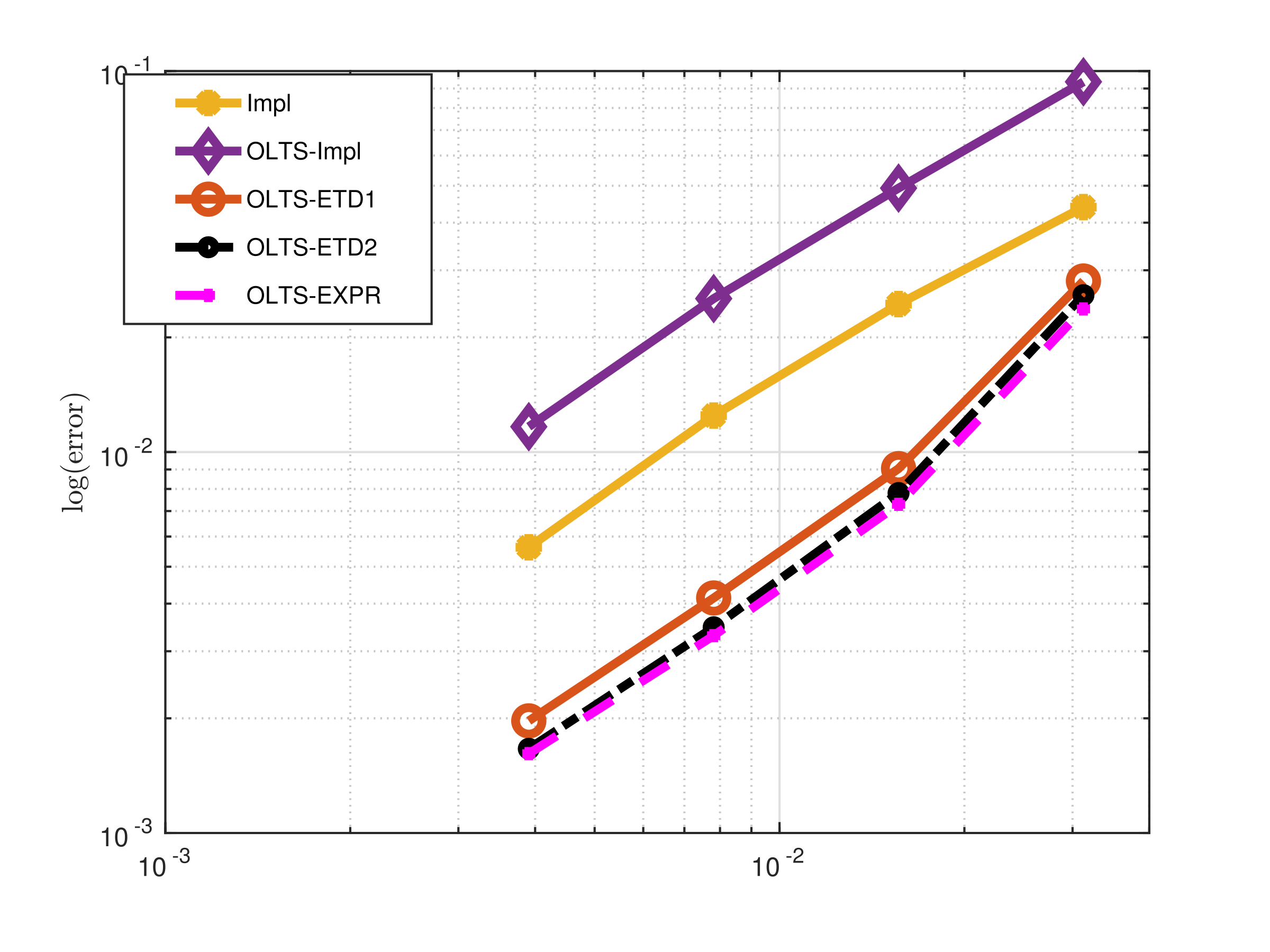
(a)

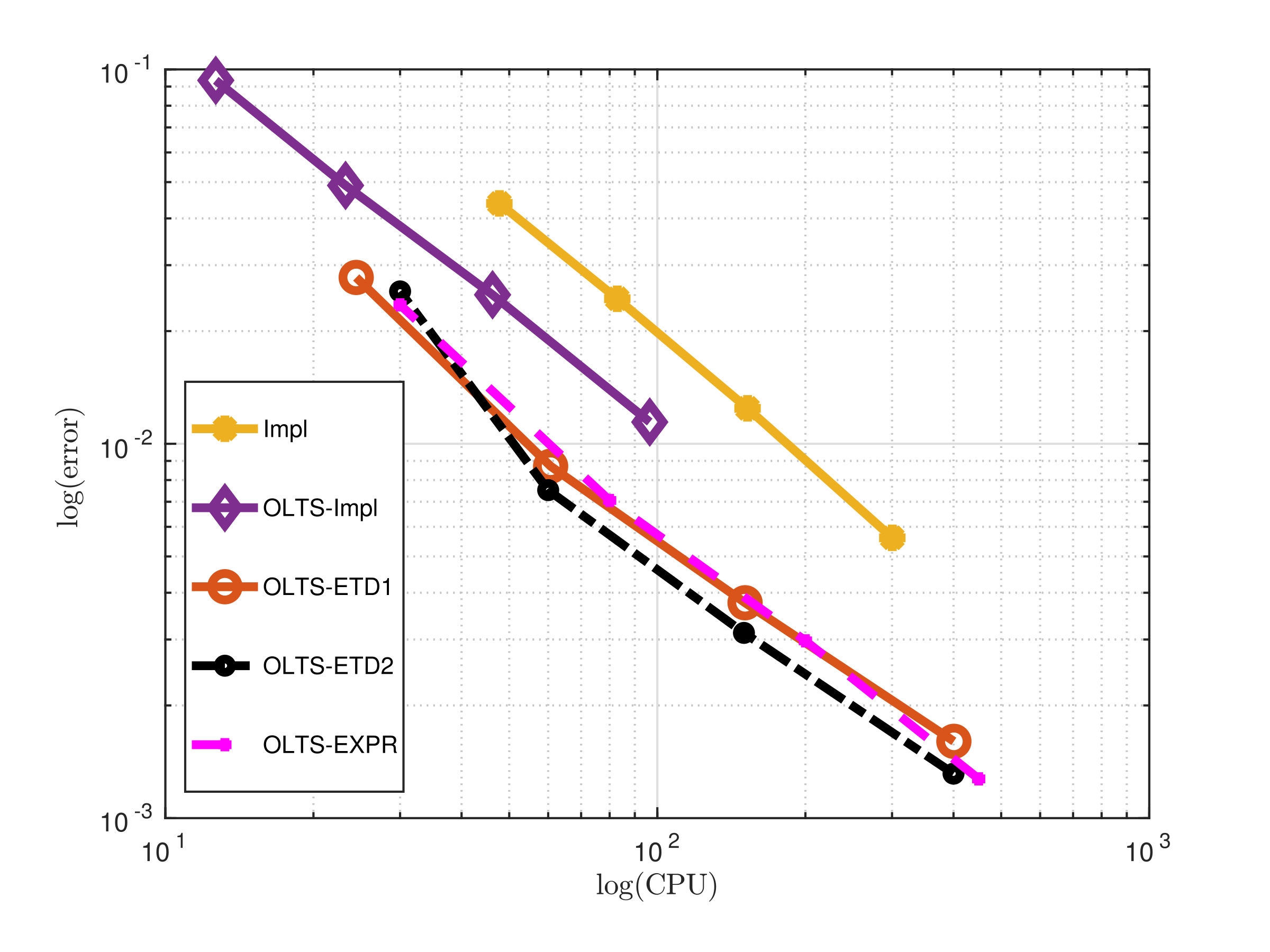
(b)

Figure 14: Convergence and efficiency of GTS-DG and OLTS-DG schemes while solving the transport of solute through a domain with fracture with presence of reaction. In (a), we plot $\log(\text{error}^{r}_{DG_{Impl}})$ and $\log(\text{error}^{r}_{DG_{OLTS-q}})$ against $\log(ht^{r})$ for all $r=0,\cdots,3$ and $q=\text{Impl}$, ETD1, ETD2, EXPR. In (b), we respectively plot $\log(\text{error}^{r}_{DG_{Impl}})$ and $\log(\text{error}^{r}_{DG_{OLTS-q}})$ against $\log(\text{CPU}^{r}_{DG_{Impl}})$ and $\log(\text{CPU}^{r}_{DG_{OLTS-q}})$ for all $r=0,\cdots,3$ and $q\in\{\text{Impl}$, ETD1, ETD2, $\text{EXPR}\}$.

Note from Figure 14(a) that the errors $\text{error}^{r}_{p}$ decrease with the time step $ht^{r}$, meaning the GTS-DG and OLTS-DG schemes, considered in this section, converge. Also, note from Figure 14(a) that

$$\text{error}^{r}_{DG_{Impl}}<\text{error}^{r}_{DG_{OLTS-Impl}}.$$ (35)

This shows that OLTS-DG schemes is less accurate compared to GTS-DG schemes. This is expected since the GTS-DG schemes, unlike the OLTS-DG schemes, consider the finest time step, uniformly on the solution domain. However, note from Figure 14(b) that the computation time is reduced enough to make the OLTS-DG schemes more efficient compared to GTS-DG schemes.

4 Conclusions

In order to efficiently capture the localized small-scale physics of DAREs on a complex geometry, we developed here two solvers, the overlap and non overlap LTS-DG schemes, based on the domain decomposition techniques, the DG spatial discretization method and the standard time integrators such as Impl, ETD, EXPR. The several numerical investigations lead to the following findings:

• When applied to Ogata and Banks problem, the numerical results of the overlap LTS-DG method show that the choice of the fast and slow components can significantly affect the accuracy of the solution. A better accuracy is obtained if the eligible sub-domains are considered in the same direction as the bulk velocity. In a high Péclet number regime, unlike in the low Péclet number regime, the size of the overlap doesn’t improve the accuracy of the overlap LTS-DG method.

• When applied to the one dimension ETO model and the two dimension transport of solute through a domain with fracture, the numerical results showed that the computation time is reduced enough to make the LTS-DG schemes proposed here more efficient compared to the GTS-DG schemes. These numerical results also showed that the non overlap LTS-DG method is more accurate and efficient compared to the overlap LTS-DG method. This is due to the fact that the needed information are more accurately computed in the case of the non overlap LTS method.

Note that for the LTS-DG methods proposed in this article, the same time integrator is used to advance locally the solution in time. Thus, to further improve our solvers, we will next investigate the case where different optimal time integrators will be used on different sub-domains to locally advance to solution in time.

References

- [1] G. Akrivis and C. Makridakis. Galerkin time-stepping methods for nonlinear parabolic equations. ESAIM: Mathematical Modelling and Numerical Analysis, 38(2):261–289, 2004.
- [2] L. Angulo, J. Alvarez, F. L. Teixeira, M. F. Pantoja, and S. G. Garcia. Causal-path local time-stepping in the discontinuous Galerkin method for Maxwell equations. Journal of Computational Physics, 256:678–695, 2014.
- [3] H. Blum, S. Lisky, and R. Rannacher. A domain splitting algorithm for parabolic problems. Computing, 49(1):11–23, 1992.
- [4] K. Böttcher and R. Rannacher. Adaptive error control in solving ordinary differential equations by the discontinuous Galerkin method. Universität Heidelberg. Interdisziplinäres Zentrum für Wissenschaftliches Rechnen [IWR], 1996.
- [5] J. Česenek and M. Feistauer. Theory of the space-time discontinuous Galerkin method for nonstationary parabolic problems with nonlinear convection and diffusion. SIAM Journal on Numerical Analysis, 50(3):1181–1206, 2012.
- [6] K. Chrysafinos and N. J. Walkington. Error estimates for discontinuous Galerkin approximations of implicit parabolic equations. SIAM journal on numerical analysis, 43(6):2478–2499, 2006.
- [7] K. Chrysafinos and N. J. Walkington. Error estimates for the discontinuous Galerkin methods for parabolic equations. SIAM Journal on Numerical Analysis, 44(1):349–366, 2006.
- [8] B. Cockburn, G. E. Karniadakis, and C.-W. Shu. The development of discontinuous Galerkin methods. In Discontinuous Galerkin Methods, pages 3–50. Springer, 2000.
- [9] R. G. Compton, E. Laborda, and K. R. Ward. Understanding voltammetry: simulation of electrode processes, volume 3 of Understanding voltammetry. Imperial College Press, 2014.
- [10] R. Courant, K. Friedrichs, and H. Lewy. On the partial difference equations of mathematical physics. IBM J. Res. Develop., 11:215–234, 1967.
- [11] J. Crank. The mathematics of diffusion. Clarendon Press, Oxford, second edition, 1975.
- [12] C. N. Dawson and Q. Du. A finite element domain decomposition method for parabolic equations. In Fourth International Symposium on Domain Decomposition Methods for PDEs, edited by R. Glowinski et al, pp255-263, SIAM, Philadelphia, 1991.
- [13] C. N. Dawson, Q. Du, and T. F. Dupont. A finite difference domain decomposition algorithm for numerical solution of the heat equation. Math. Comp., 57(195):63–71, 1991.
- [14] C. N. Dawson and T. F. Dupont. Explicit/implicit conservative Galerkin domain decomposition procedures for parabolic problems. mathematics of computation, 58(197):21–34, 1992.
- [15] J. V. der Vegt and H. V. der Ven. Space-time discontinuous Galerkin finite element method with dynamic grid motion for inviscid compressible flows: I. general formulation. Journal of Computational Physics, 182(2):546–585, 2002.
- [16] J. V. der Vegt and H. V. der Ven. Space-time discontinuous Galerkin finite element method with dynamic grid motion for inviscid compressible flows: Ii. efficient flux quadrature. Computer methods in applied mechanics and engineering, 191(41):4747–4780, 2002.
- [17] J. Diaz and M. J. Grote. Energy conserving explicit local time stepping for second-order wave equations. SIAM Journal on Scientific Computing, 31(3):1985–2014, 2009.
- [18] J. Diaz and M. J. Grote. Multi-level explicit local time-stepping methods for second-order wave equations. Computer methods in applied mechanics and engineering, 291:240–265, 2015.
- [19] V. Dolejší and M. Feistauer. Discontinuous Galerkin method. Analysis and Applications to Compressible Flow, 48, 2015.
- [20] M. Dryja et al. Substructuring methods for parabolic problems. In Proceedings of the Fourth International Symposium on Domain Decomposition Methods for Partial Differential Equations, pages 264–271, 1991.
- [21] M. Dumbser, M. Käser, and E. F. Toro. An arbitrary high-order discontinuous Galerkin method for elastic waves on unstructured meshes-v. local time stepping and p-adaptivity. Geophysical Journal International, 171(2):695–717, 2007.
- [22] C. Engstler and C. Lubich. Multirate extrapolation methods for differential equations with different time scales. Computing, 58(2):173–185, 1997.
- [23] K. Eriksson and C. Johnson. Adaptive finite element methods for parabolic problems i: A linear model problem. SIAM Journal on Numerical Analysis, 28(1):43–77, 1991.
- [24] K. Eriksson, C. Johnson, and A. Logg. Adaptive computational methods for parabolic problems. Wiley Online Library, 2004.
- [25] D. Estep. A posteriori error bounds and global error control for approximation of ordinary differential equations. SIAM Journal on Numerical Analysis, 32(1):1–48, 1995.
- [26] D. Estep and S. Larsson. The discontinuous Galerkin method for semilinear parabolic problems. RAIRO-Modélisation mathématique et analyse numérique, 27(1):35–54, 1993.
- [27] R. E. Ewing, R. D. Lazarov, and A. T. Vassilev. Finite difference scheme for parabolic problems on composite grids with refinement in time and space. SIAM Journal on Numerical Analysis, 31(6):1605–1622, 1994.
- [28] I. Faille, F. Nataf, F. Willien, and S. Wolf. Two local time stepping schemes for parabolic problems. In Multiresolution and adaptive methods for convection-dominated problems, volume 29 of ESAIM Proc., pages 58–72. EDP Sci., Les Ulis, 2009.
- [29] I. Faille, F. Nataf, F. Willien, and S. Wolf. Two local time stepping schemes for parabolic problems. In ESAIM: proceedings, volume 29, pages 58–72. EDP Sciences, 2009.
- [30] F. Fambri, M. Dumbser, and O. Zanotti. Space-time adaptive ader-dg schemes for dissipative flows: Compressible Navier-Stokes and resistive mhd equations. Computer Physics Communications, 220:297–318, 2017.
- [31] M. Feistauer, J. Hájek, and K. Švadlenka. Space-time discontinuos Galerkin method for solving nonstationary convection-diffusion-reaction problems. Applications of Mathematics, 52(3):197–233, 2007.
- [32] M. Feistauer, V. Kučera, K. Najzar, and J. Prokopová. Analysis of space–time discontinuous Galerkin method for nonlinear convection–diffusion problems. Numerische Mathematik, 117(2):251–288, 2011.
- [33] M. Feistauer, V. Kučera, K. Najzar, and J. Prokopová. Analysis of space-time discontinuous Galerkin method for nonlinear convection-diffusion problems. Numerische Mathematik, 117(2):251–288, 2011.
- [34] A. Fick. Ueber diffusion. Annalen der Physik, 170(1):59–86, 1855.
- [35] A. Fick. On liquid diffusion. Journal of Membrane Science, 100(1):33–38, 1995.
- [36] M. J. Gander and C. Rohde. Overlapping Schwarz waveform relaxation for convection-dominated nonlinear conservation laws. SIAM journal on Scientific Computing, 27(2):415–439, 2005.
- [37] C. W. Gear and D. Wells. Multirate linear multistep methods. BIT Numerical Mathematics, 24(4):484–502, 1984.
- [38] G. H. Hardy and E. M. Wright. An introduction to the theory of numbers. The Clarendon Press, Oxford University Press, New York, fifth edition, 1979.
- [39] C. Johnson. Error estimates and adaptive time-step control for a class of one-step methods for stiff ordinary differential equations. SIAM Journal on Numerical Analysis, 25(4):908–926, 1988.
- [40] C. M. Klaij, J. J. van der Vegt, and H. van der Ven. Space–time discontinuous Galerkin method for the compressible Navier-Stokes equations. Journal of Computational Physics, 217(2):589–611, 2006.
- [41] A. H. Kouevi. Numerical Methods for Stiff Systems. Phd, University of Heriot-Watt, 2017.
- [42] Y. M. Laevsky. On the domain decomposition method for parabolic problems. Bull. Novosibirsk Comput. Center, 1:41–62, 1993.
- [43] P. Lesaint and P. A. Raviart. On a finite element method for solving the neutron transport equation. Publications mathématiques et informatique de Rennes, (S4):1–40, 1974.
- [44] F. Lörcher, G. Gassner, and C.-D. Munz. A discontinuous Galerkin scheme based on a space–time expansion. I. inviscid compressible flow in one space dimension. Journal of Scientific Computing, 32(2):175–199, 2007.
- [45] T. P. Mathew, P. L. Polyakov, G. Russo, and J. Wang. Domain decomposition operator splittings for the solution of parabolic equations. SIAM Journal on Scientific Computing, 19(3):912–932, 1998.
- [46] A. Ogata and R. Banks. A Solution of the Differential Equation of Longitudinal Dispersion in Porous Media. Fluid movement in earth materials. U.S. Government Printing Office, 1961.
- [47] P. olof Persson, A. Edelman, R. R. Rosales, and P. olof Persson. Mesh Generation for Implicit Geometries. PhD thesis, Department of Mathematics, MIT, 2005.
- [48] P. olof Persson and G. Strang. A simple mesh generator in matlab. SIAM Review, 46:2004, 2004.
- [49] J. R. Rice. Split Runge-Kutta method for simultaneous equations. J. Res. Nat. Bur. Standards Sect. B, 64B:151–170, 1960.
- [50] M. Rietmann, D. Peter, O. Schenk, B. Uçar, and M. Grote. Load-balanced local time stepping for large-scale wave propagation. In Parallel and Distributed Processing Symposium (IPDPS), 2015 IEEE International, pages 925–935. IEEE, 2015.
- [51] D. Schötzau. hp-DGFEM for parabolic evolution problems: applications to diffusion and viscous incompressible fluid flow. na, 1999.
- [52] D. Schötzau and C. Schwab. An hp a priori error analysis of the DG time-stepping method for initial value problems. Calcolo, 37(4):207–232, 2000.
- [53] S. Skelboe and P. U. Andersen. Stability properties of backward Euler multirate formulas. SIAM journal on scientific and statistical computing, 10(5):1000–1009, 1989.
- [54] J. Sudirham, J. Van Der Vegt, and R. Van Damme. Space–time discontinuous Galerkin method for advection–diffusion problems on time-dependent domains. Applied numerical mathematics, 56(12):1491–1518, 2006.
- [55] A. Taube, M. Dumbser, C.-D. Munz, and R. Schneider. A high-order discontinuous Galerkin method with time-accurate local time stepping for the Maxwell equations. International Journal of Numerical Modelling: Electronic Networks, Devices and Fields, 22(1):77–103, 2009.
- [56] V. A. Titarev and E. F. Toro. ADER: Arbitrary high order godunov approach. Journal of Scientific Computing, 17(1):609–618, 2002.
- [57] P. Vabishchevich. Parallel domain decomposition algorithms for time-dependent problems of mathematical physics. Advances in Numerical Methods and Applications, pages 293–299, 1994.
- [58] P. N. Vabishchevich. Two-component domain decomposition scheme with overlapping subdomains for parabolic equations. Journal of Computational and Applied Mathematics, 2017.
- [59] M. F. Wheeler. An elliptic collocation-finite element method with interior penalties. SIAM J. Numer. Anal., 15(1):152–161, 1978.