VQVAE Unsupervised Unit Discovery
and Multi-scale Code2Spec Inverter
for Zerospeech Challenge 2019

Abstract

We describe our submitted system for the ZeroSpeech Challenge 2019. The current challenge theme addresses the difficulty of constructing a speech synthesizer without any text or phonetic labels and requires a system that can (1) discover subword units in an unsupervised way, and (2) synthesize the speech with a target speaker’s voice. Moreover, the system should also balance the discrimination score ABX, the bit-rate compression rate, and the naturalness and the intelligibility of the constructed voice. To tackle these problems and achieve the best trade-off, we utilize a vector quantized variational autoencoder (VQ-VAE) and a multi-scale codebook-to-spectrogram (Code2Spec) inverter trained by mean square error and adversarial loss. The VQ-VAE extracts the speech to a latent space, forces itself to map it into the nearest codebook and produces compressed representation. Next, the inverter generates a magnitude spectrogram to the target voice, given the codebook vectors from VQ-VAE. In our experiments, we also investigated several other clustering algorithms, including K-Means and GMM, and compared them with the VQ-VAE result on ABX scores and bit rates. Our proposed approach significantly improved the intelligibility (in CER), the MOS, and discrimination ABX scores compared to the official ZeroSpeech 2019 baseline or even the topline.

1 Introduction

Current spoken language technologies only cover about two percent of the world’s languages. This is because most groundworks require a large amount of paired data resources, including a sizeable collection of spoken audio data and corresponding text transcription. On the other hand, most of the world’s languages are severely under-resourced, some of which even lack a written form. Zero resource speech research is an extreme case from low-resourced approaches that learn the elements of a language solely from untranscribed raw audio data. This completely unsupervised technique attempts to mimic the early language acquisition of humans. The zero resource speech challenge (ZeroSpeech) [1, 2, 3] is directly addressing this issue and offers participants the opportunity to advance the state-of-the-art in the core tasks of zero resource speech technology.

In ZeroSpeech 2015 and 2017, the goal was to discover an appropriate speech representation of the underlying language of a dataset [1, 2]. The ZeroSpeech 2019 [3] challenge confronts the problem of constructing a speech synthesizer without any text or phonetic labels: TTS without T. The task requires the full system not only to discover subword units in an unsupervised way but also to re-synthesize the speech with a same content to a different target speaker. It includes both ASR and TTS components. In this paper, we describe our submitted system for the ZeroSpeech Challenge 2019 and focus on constructing end-to-end systems.

The top performances in discovering speech representation in ZeroSpeech 2015 and 2017 are dominated by a Bayesian non-parametric approach with unsupervised cluster speech features using a Dirichlet process Gaussian mixture model (DPGMM) [4, 5]. However, the DPGMM model is too sensitive to acoustic variations and often produces too many subword units and a relatively high-dimensional posteriogram, which implies high computational cost for learning and inference as well as more tendencies for overfitting [6]. Therefore it is difficult to synthesize speech waveform from the resulting DPGMM-based acoustic units.

To tackle these problems and achieve the best trade-off, an optimization method is required to balance and improve both components. Recently, Tjandra et al. [7, 8, 9] proposed a machine speech chain (see Figure 1) that enables ASR and TTS to assist each other when they receive unpaired data by allowing them to infer the missing pair and optimize both models with reconstruction loss. However, since the architecture is based on an attention-based sequence-to-sequence framework that transforms from a dynamic-length input into a dynamic-length output without decoding at the frame-level (one symbol per frame), it is less suitable for this challenge.

Inspired by a similar idea, we propose to utilize a frame-based vector quantized variational autoencoder (VQ-VAE) [10] and a multi-scale codebook-to-spectrogram (Code2Spec) inverter trained by mean square error (MSE) and adversarial loss. VQ-VAE extracts the speech to a latent space and forces itself to map onto the nearest codebook, leading to compressed representation. Next, the inverter generates a magnitude spectrogram to the target voice, given the codebook vector from VQ-VAE. In our experiments, we also investigate other clustering algorithms such as K-Means and GMM and compare them with the VQ-VAE result on ABX scores and bit rate.

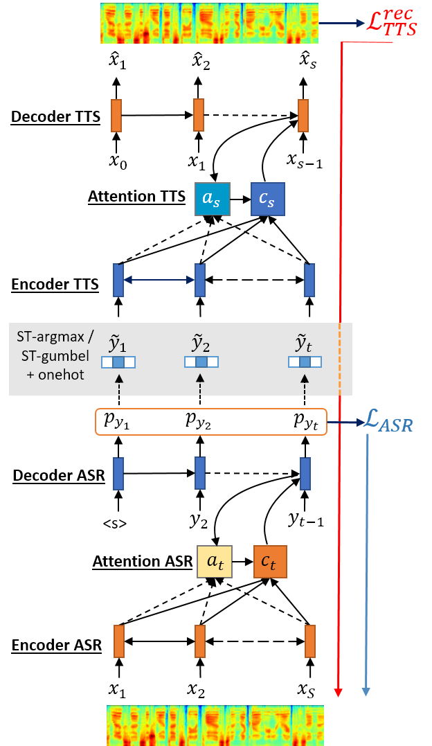
Figure 1: Speech chain model consists of an ASR and a TTS module. Given speech features $\mathbf{x}$, the ASR generates a transcription. The TTS reconstructs the speech features based on the transcription and calculates the reconstruction loss ${\cal L}^{rec}_{tts}$.

2 Vector Quantized Variational Autoencoder (VQ-VAE)

A vector quantized variational autoencoder (VQ-VAE) [10] is a variant of variational autoencoder architecture. It has several differences compared to a standard autoencoder or a variational autoencoder [11] (VAE). First, the encoder generates discrete latent variables instead of continuous latent variables to represent the input data. Second, instead of one-to-one mapping between the input data and the latent variables, VQ-VAE forces the latent variables to be represented by the closest codebook vector.

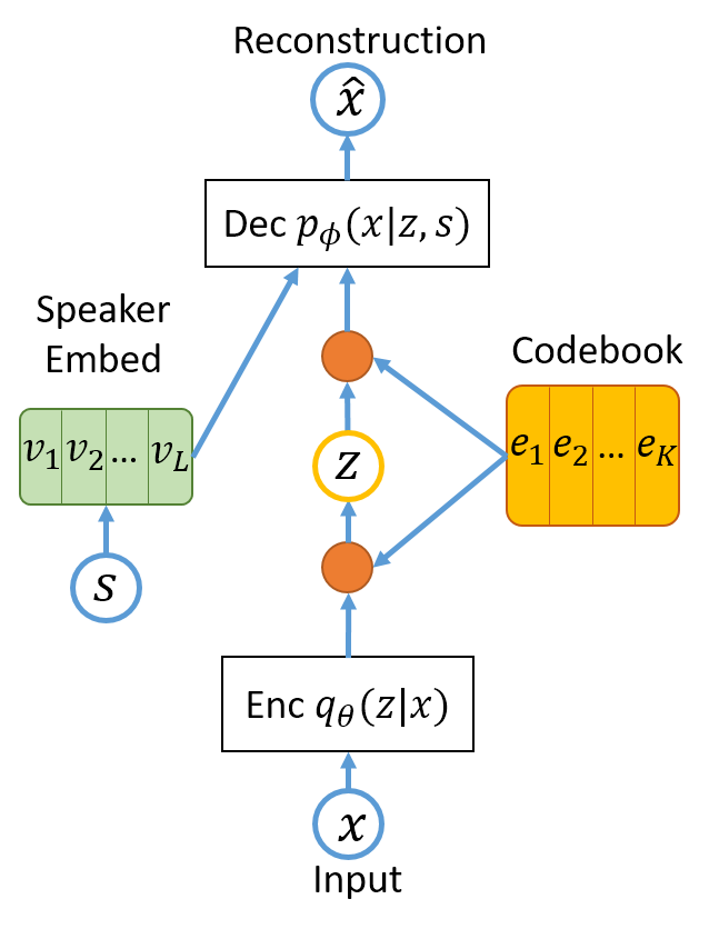
Figure 2: Conditional VQ-VAEs consist of four main modules: encoder $q_{\theta}(z|x)$, decoder $p_{\phi}(x|z,s)$, codebooks $E=[e_{1},..,e_{K}]$, and speaker embedding $V=[v_{1},..,v_{L}]$.

Figure 2 illustrates the encoding and decoding processes from the conditional VQ-VAE model. Here $x$ is the input data, $s\in\{1,..,L\}$ is the speaker ID that is related to $x$, $z\in\{1,..,K\}$ is a discrete latent variable, and $\hat{x}$ is the reconstructed input. Encoder $q_{\theta}(z|x)$ and decoder $p_{\phi}(x|z,s)$ can be represented by any differentiable transformation (e.g., linear, convolution, recurrent layer) parameterized by $\{\phi,\theta\}$. Codebook $E=[e_{1},e_{2},..,e_{K}]\in\mathbb{R}^{K\times D_{e}}$ is a collection of $K$ continuous codebook vectors with $D_{e}$ dimensions. Speaker embedding $V=[v_{1},v_{2},...,v_{L}]\in\mathbb{R}^{L\times D_{v}}$ is speaker embedding to map speaker ID $s$ into a continuous representation. In the encoding step, encoder $q_{\theta}(z|x)$ projects input $x$ into continuous representation $\hat{z}\in\mathbb{R}^{D_{e}}$. Posterior distributions $q_{\theta}(z|x)$ are generated by a discretization process:

$$q_{\theta}(z=c|x) =\begin{cases}1\quad\text{if }\,c=\operatorname*{argmin}_{i}\|\hat{z}-e_{i}\|_{2}\\ 0\quad\text{else }\end{cases}$$ (1)

$$e_{c} =\sum_{i=1}^{K}q_{\theta}(z=i|x)\,e_{i}.$$ (2)

In the discretization process, we choose closest codebook vector $e_{c}$ based on the index of the closest distance (e.g., L2-norm distance) from continuous representation $\hat{z}$. To decode the data, we use codebook $e_{c}$ and speaker embedding $v_{s}$ and feed both into decoder $p_{\phi}(x|z,s)=p_{\phi}(x|e_{c},v_{s})$ to reconstruct original data $\hat{x}$.

In VQ-VAE, we formulate the training objective:

$$\mathcal{L}_{VQ}=-\log p_{\phi}(x|z,s)+\|\text{sg}(\hat{z})-e_{c}\|_{2}^{2}+\gamma\|\hat{z}-\text{sg}(e_{c})\|_{2}^{2},$$ (3)

where function $\text{sg}(\cdot)$ stops the gradient, defined as:

$$x=sg(x);\quad\frac{\partial\,\text{sg}(x)}{\partial\,x}=0.$$ (4)

There are three terms in loss $\mathcal{L}_{VQ}$. The first is a negative log-likelihood that resembles a reconstruction loss and optimizes the encoder and decoder parameters. The second optimizes codebook vectors $E$, named codebook loss. The third forces the encoder to generate a representation near the codebook, called commitment loss. Coefficient $\gamma$ is used to scale the commitment loss.

3 Codebook-to-Spectrogram Inverter

The codebook-to-spectrogram (Code2Spec) inverter is a module that reconstructs the speech signal representation (e.g., linear magnitude spectrogram) $M=[m[1],m[2],...,m[T_{s}]]\in\mathbb{R}^{T_{s}\times D_{m}}$, given a sequence of codebook $[e[1],e[2],...,e[T_{z}]]\in\mathbb{R}^{T_{z}\times D_{e}}$.

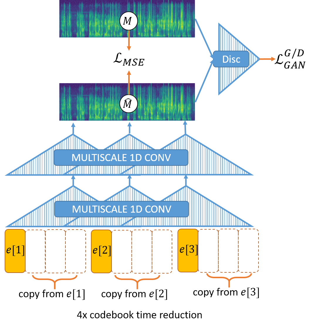
Figure 3: Code-to-speech inverter: given a sequence of codebook $\left[e[1],e[2],..,e[T_{z}]\right]$, we duplicate each codebook based on compression ratio $r=4$ and apply multiple layers of multi-scale 1D convolution + LeakyReLU activation function to predict the target voice linear spectrogram $\hat{M}$.

In Fig. 3, we illustrate our code-to-speech inverter model. The length of codebook sequence $T_{z}$ might be shorter than $T_{s}$, depending on the VQ-VAE encoder $q_{\theta}(z|x)$ model. Therefore, for an identical length between the codebook and speech representation sequences, we need to copy $r=T_{s}/T_{z}$ times for each codebook $e[t];\,\forall t\in[1..T_{z}]$. Later, duplicated codebook sequences $[e[1],e[1],..,e[T_{z}],e[T_{z}]]\in\mathbb{R}^{T_{s}\times D_{e}}$ are given to the inverter that consists of multiple layers of multi-scale 1D convolution, batch-normalization [12], and LeakyReLU [13] non-linearity. In addition to the inverter, we also have a discriminator module. The discriminator predicts whether the given spectrogram is real data or is generated by the inverter, which generates a realistic spectrogram to deceive the discriminator [14, 15, 16]. The Code2Spec inverter has several training objectives:

$$\hat{M} =\text{Code2Spec}([e[1],e[1],..,e[T_{z}],e[T_{z}]])$$ (5)

$$\mathcal{L}_{MSE} =\|M-\hat{M}\|_{2}^{2}$$ (6)

$$\mathcal{L}_{GAN}^{G} =\begin{cases}-\text{Disc}(\hat{M})&\text{WGAN \cite[cite]{[\@@bibref{}{arjovsky2017wasserstein}{}{}]}}\\ (\text{Disc}(\hat{M})-1)^{2}&\text{LSGAN \cite[cite]{[\@@bibref{}{mao2017least}{}{}]}}\end{cases}$$ (7)

$$\mathcal{L}_{GAN}^{D} =\begin{cases}\text{Disc}(\hat{M})-\text{Disc}(M)&\text{WGAN}\\ \text{Disc}(\hat{M})^{2}+(\text{Disc}(M)-1)^{2}&\text{LSGAN}\end{cases}$$ (8)

After we define the multiple objectives for training, we update each module parameter $\theta_{C2S}$ and $\theta_{Disc}$ with the following equation:

$$\theta_{C2S} = \text{Optim}(\theta_{C2S},\nabla_{\theta_{C2S}}(\alpha{\cal L}_{MSE}+\beta{\cal L}_{GAN}^{G}))$$ (9)

$$\theta_{Disc} = \text{Optim}(\theta_{Disc},\nabla_{\theta_{Dssc}}({\cal L}_{GAN}^{D})),$$ (10)

where Optim($\cdot,\cdot$) is a gradient optimization function (e.g., SGD, Adam [19]), $\alpha$ and $\beta$ is the coefficient to balance the loss between the MSE and the adversarial loss. In the inference stage, given the predicted linear magnitude spectrogram $\hat{M}$, we reconstruct the missing phase spectrogram with the Griffin-Lim algorithm [20] and applied the inverse short-term Fourier transform (STFT) to generate the waveform.

4 Experiment

In this section, we describe the feature extraction, the preliminary models, and our proposed models for this challenge. All of the results were evaluated using evaluate.sh from the English test set.

4.1 Experimental Set-up

There are two datasets for two languages, English data for the development dataset, and a surprise Austronesian language for the test dataset. Each language dataset contains subset datasets: (1) a Voice Dataset for speech synthesis, (2) a Unit Discovery Dataset, (3) an Optional Parallel Dataset from the target voice to another speaker voice, and (4) a Test Dataset. The source corpora of the surprise language are describe here [21, 22], and further details can be found here [3]. In this work, we only use (1)-(2) for training and (4) for testing.

For the speech input, we experimented with several feature types, such as Mel-spectrogram (80 dimensions, 25-ms window size, 10-ms time-steps) and MFCC (13 dimensions$+\Delta+\Delta^{2}$ (total=39 dimensions), 25-ms window size, 10-ms time-steps). Both MFCC and Mel-spectrogram are generated by the Librosa package [23].

4.2 Official baseline and topline model

ZeroSpeech 2019 provides official baselines and toplines. The baseline consists of a pipeline with a simple acoustic unit discovery system based on DPGMM and a speech synthesizer based on Merlin, and the topline uses gold phoneme transcription to train a phoneme-based ASR system with Kaldi and a phoneme-based TTS with Merlin. The performance is shown in Table 1.

Table 1: Official ZeroSpeech 2019 baseline and topline result.

Feature	ABX	Bit rate
Baseline	35.63	71.98
Topline	29.85	37.73

4.3 Preliminary model

We started to explore this challenge using a simpler method and gradually increased our model’s complexity.

4.3.1 Direct feature representation

We directly evaluated the ABX and the bit rate of Mel-spectrogram and MFCC as speech representations. In Table 2, we report each feature extraction method with respect to their ABX and bit rates. In our preliminary experiments, MFCC produced better performances on the ABX metric than the Mel-spectrogram. Therefore, for the rest of our discussion, we only focus on utilizing MFCC features. However, even the MFCC has better ABX score, the bit rate still remains too high.

Table 2: Direct feature representation (MFCC and Mel-spec) result on ABX with DTW cosine distance and bit rate.

Feature	ABX	Bit rate
Mel-Spec	30.291	1738.38
MFCC	21.114	1737.47

4.3.2 K-Means

We trained Minibatch K-Means (with scikit-learn toolkit [24]) on the MFCC feature and varied the cluster size: 64, 128, 256. We represent a data point (a speech frame) K-Means by using the closest centroid vector to the data frame and calculate the ABX with the DTW cosine. Table 3 reports all the models and their configurations with respect to their ABX and bit rate.

Table 3: K-Means continuous representation result on ABX and bit rate. C is codebook size, T is time reduction.

Model	ABX / Bitrate
K-Means (cont, DTW cos)	#C	1T	2T	4T
	64	23.56 / 553	25.97 / 280	29.41 / 136
	128	23.16 / 649	24.24 / 321	28.12 / 161
	256	21.90 / 744	23.73 / 369	27.17 / 182

4.3.3 Gaussian Mixture Model (GMM)

We trained GMM with diagonal covariance matrices (with scikit-learn toolkit [24]) on the MFCC features. We varied the number of mixtures: 64, 128, and 256. We represent a data point (a speech frame) with the posterior probability from each component with a Bayes rule $p(z|x)\propto p(x|z)p(z)$ and calculate the ABX with DTW KL-divergence. In Table 4, we report all of the models and their configurations with respect to their ABX and bit rate.

Table 4: GMM posterior representation result on ABX and bit rate. C is codebook size, T is time reduction

Model	ABX / Bit rate
GMM (post, DTW KL)	#C	1T	2T	4T
	64	20.81 / 1647	22.67 / 676	29.82 / 257
	128	19.61 / 1705	23.06 / 704	31.19 / 281
	256	18.93 / 1691	23.39 / 757	32.99 / 306

4.4 Proposed model

Table 5: VQ-VAE codebook representation result on ABX and bit rate. C is codebook size, T is time reduction. Blue font denotes our submitted system.

Model	ABX / Bit rate
	#CL	1T	2T	4T	8T
	64	27.46 / 606	25.51 / 302	26.15 / 138	28.81 / 70
	128	27.65 / 686	24.29 / 347	25.04 / 165	30.87 / 79
	256	27.63 / 787	24.37 / 349	24.17 / 184	30.51 / 79
VQ-VAE (cont, DTW cos)	512	27.69 / 871	23.59 / 400	24.63 / 180	32.02 / 74

4.4.1 VQ-VAE

Next we describe our encoder and decoder architecture in Fig. 4 with four times the sequence length reduction. For the input and output targets, we use the MFCC features and explore different stride sizes to reduce the time length from 1, 2, 4, 8. We use speaker embedding with 32 dimensions and codebook embedding with 64 dimensions. We varied the number of codebooks: 64, 128, 256, 512. Batch normalization [12] and LeakyReLU [13] activation were applied to every layer, except the last encoder and decoder layer. The decoder input is a concatenation between codebook and speaker embedding in the channel axis. We set commitment loss coefficient $\gamma=0.25$.

4.4.2 Multi-scale Code2Spec inverter

In Fig. 4, we describe our inverter architecture. Our input is a codebook sequence with 64 dimensions and our target output is a sequence of linear magnitude spectrogram with 1025 dimensions. The first four layers have multiple kernels with different sizes across the time-axis. All convolution layers have stride = 1 and the “same” padding. Batch normalization and LeakyReLU activation are applied to every layer, except the last one before the output prediction. For the adversarial loss, we found LSGAN is stabler, thus LSGAN with $\beta=1$ is used in every model. We independently trained the inverter to generate a voice target speaker with a train/voice set. We have two inverters for the English set and one for the surprise set.

4.4.3 Model training

We used Adam [19] as our first-order optimizer for both VQ-VAE and the Code2Spec inverter. All of our models are implemented with PyTorch [25] framework.

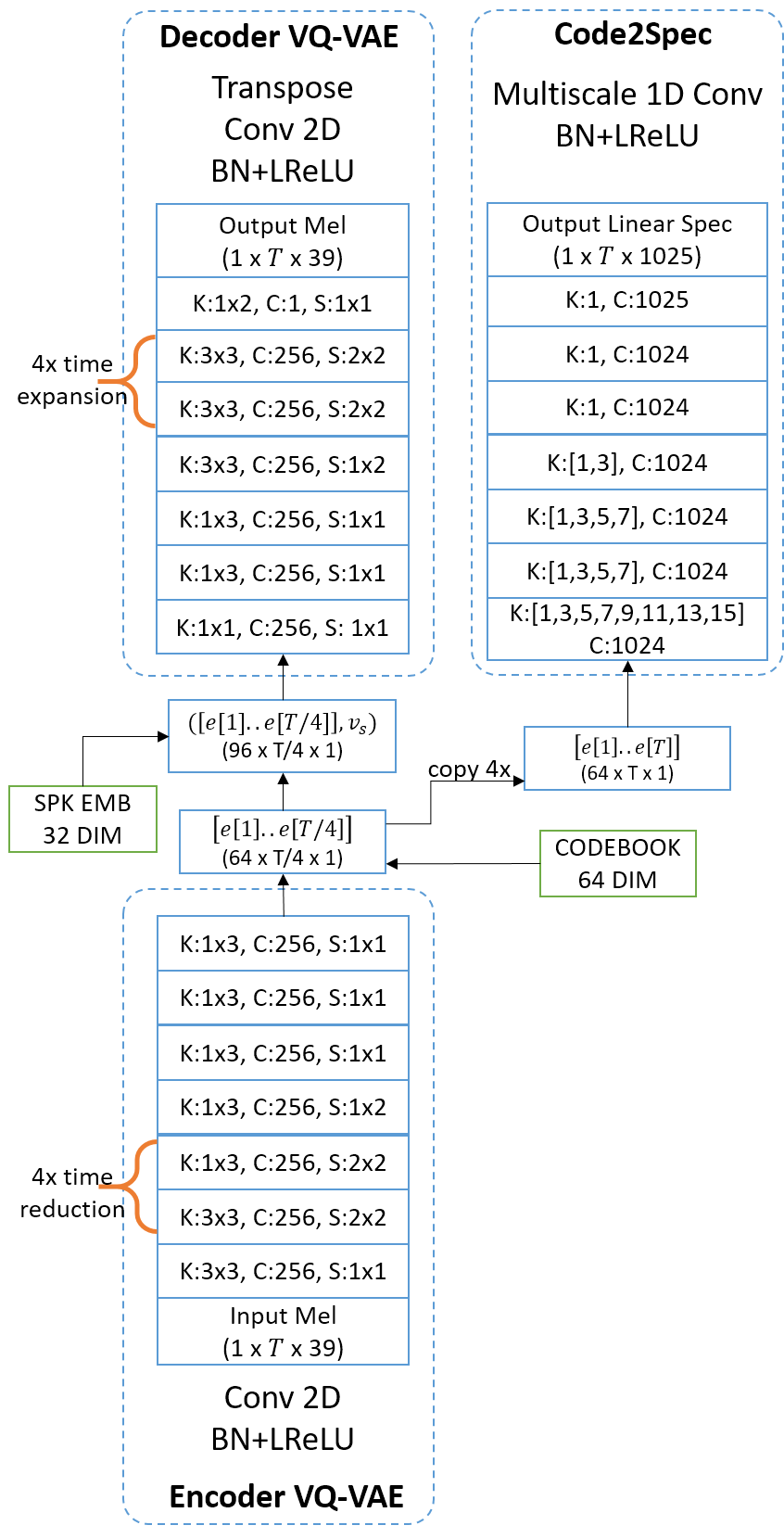
Figure 4: Left: VQ-VAE encoder and decoder architecture with 4x time reduction (based on stride size in encoder layer). Right: Code2Spec architecture. Definition: K is kernel size, C is output channel, S is stride size, and T is input frame length. K:3x3 denotes 2D convolution with 3x3 kernel size across time and frequency axis, K:[1,3,5,7] denotes 1D convolution with 4 different kernel size (1, 3, 5, 7) across time-axis.

4.4.4 Results and Discussion

Table 5 reports all models and their configurations with respect to their ABX and bit rate. Considering the balance between the discrimination score ABX and the bit-rate compression rate, we submitted two proposed systems: (1) 256 codebooks and 4 stride size to reduce the time length and (2) 256 codebooks and 2 stride size to reduce the time length.

We also attempted further enhancement of the synthesized voice using several techniques, such as WaveNet [26, 27] and GAN-based voice conversion [28]. WaveNet decoder is conditioned by frame-wise linguistic features or acoustic features with a 5ms timeshift (80 times smaller than the speech samples). As the sample rate of the codebook embeddings of our system was 320 times smaller than the speech samples, the Wavenet couldn’t produced satisfying result. GANs are known to be effective for achieving high-quality voice conversion with clean input data [29, 30]. However, our task is more challenging due to the fact that our generated voice will always have some distortion. Therefore, GAN-based voice conversion approach failed to improve our performance. As a future work, we will investigate the use of GAN-based speech enhancement [31] approaches to further improve our results.

5 Conclusions

We described our approach for the ZeroSpeech Challenge 2019 for unsupervised unit discovery. We explored many different possibilities: feature extraction, clustering algorithm, and embedding representation. For our final submission, we utilized VQ-VAE to extract a sequence of codebook vectors. The codebook generated by VQ-VAE has a better trade-off between ABX and the bit rate compared to the other models such as K-Means, GMM, or direct feature representation. To reconstruct speech from the codebook, we trained a Code2Spec inverter to generate a corresponding linear magnitude spectrogram. The combination between VQ-VAE and Code2Spec significantly improved the intelligibility (in CER), the MOS, and the discrimination ABX scores compared to the official ZeroSpeech 2019 baseline or even the topline.

6 Acknowledgements

Part of this work was supported by JSPS KAKENHI Grant Numbers JP17H06101 and JP17K00237.

References

- [1] M. Versteegh, R. Thiolliere, T. Schatz, X. N. Cao, X. Anguera, A. Jansen, and E. Dupoux, “The zero resource speech challenge 2015,” in Sixteenth Annual Conference of the International Speech Communication Association, 2015.
- [2] E. Dunbar, X. N. Cao, J. Benjumea, J. Karadayi, M. Bernard, L. Besacier, X. Anguera, and E. Dupoux, “The zero resource speech challenge 2017,” in 2017 IEEE Automatic Speech Recognition and Understanding Workshop (ASRU), pp. 323–330, IEEE, 2017.
- [3] J. K. M. B. J. B. X.-N. C. L. M. C. D. L. O. A. W. B. L. B. S. S. E. D. E. Dunbar, R. Algayres, “The zero resource speech challenge 2019: TTS without T,” in Twentieth Annual Conference of the International Speech Communication Association (INTERSPEECH 2019), 2019.
- [4] H. Chen, C.-C. Leung, L. Xie, B. Ma, and H. Li, “Parallel inference of dirichlet process gaussian mixture models for unsupervised acoustic modeling: A feasibility study,” in Sixteenth Annual Conference of the International Speech Communication Association, 2015.
- [5] M. Heck, S. Sakti, and S. Nakamura, “Feature optimized dpgmm clustering for unsupervised subword modeling: A contribution to zerospeech 2017,” in 2017 IEEE Automatic Speech Recognition and Understanding Workshop (ASRU), pp. 740–746, IEEE, 2017.
- [6] B. Wu, S. Sakti, J. Zhang, and S. Nakamura, “Optimizing DPGMM clustering in zero-resource setting based on functional load,” in Proc. The 6th Intl. Workshop on Spoken Language Technologies for Under-Resourced Languages, pp. 1–5.
- [7] A. Tjandra, S. Sakti, and S. Nakamura, “Listening while speaking: Speech chain by deep learning,” in 2017 IEEE Automatic Speech Recognition and Understanding Workshop (ASRU), pp. 301–308, IEEE, 2017.
- [8] A. Tjandra, S. Sakti, and S. Nakamura, “Machine speech chain with one-shot speaker adaptation,” Proc. Interspeech 2018, pp. 887–891, 2018.
- [9] A. Tjandra, S. Sakti, and S. Nakamura, “End-to-end feedback loss in speech chain framework via straight-through estimator,” in 2019 IEEE International Conference on Acoustics, Speech and Signal Processing (ICASSP), p. to appear, IEEE, 2019.
- [10] A. van den Oord, O. Vinyals, et al., “Neural discrete representation learning,” in Advances in Neural Information Processing Systems, pp. 6306–6315, 2017.
- [11] D. P. Kingma and M. Welling, “Auto-encoding variational bayes,” arXiv preprint arXiv:1312.6114, 2013.
- [12] S. Ioffe and C. Szegedy, “Batch normalization: Accelerating deep network training by reducing internal covariate shift,” arXiv preprint arXiv:1502.03167, 2015.
- [13] A. L. Maas, A. Y. Hannun, and A. Y. Ng, “Rectifier nonlinearities improve neural network acoustic models,” in in ICML Workshop on Deep Learning for Audio, Speech and Language Processing, Citeseer, 2013.
- [14] I. Goodfellow, J. Pouget-Abadie, M. Mirza, B. Xu, D. Warde-Farley, S. Ozair, A. Courville, and Y. Bengio, “Generative adversarial nets,” in Advances in neural information processing systems, pp. 2672–2680, 2014.
- [15] Y. Saito, S. Takamichi, and H. Saruwatari, “Statistical parametric speech synthesis incorporating generative adversarial networks,” IEEE/ACM Transactions on Audio, Speech, and Language Processing, vol. 26, pp. 84–96, Jan 2018.
- [16] T. Kaneko, H. Kameoka, N. Hojo, Y. Ijima, K. Hiramatsu, and K. Kashino, “Generative adversarial network-based postfilter for statistical parametric speech synthesis,” in 2017 IEEE International Conference on Acoustics, Speech and Signal Processing (ICASSP), pp. 4910–4914, IEEE, 2017.
- [17] M. Arjovsky, S. Chintala, and L. Bottou, “Wasserstein gan,” arXiv preprint arXiv:1701.07875, 2017.
- [18] X. Mao, Q. Li, H. Xie, R. Y. Lau, Z. Wang, and S. Paul Smolley, “Least squares generative adversarial networks,” in Proceedings of the IEEE International Conference on Computer Vision, pp. 2794–2802, 2017.
- [19] D. P. Kingma and J. Ba, “Adam: A method for stochastic optimization,” arXiv preprint arXiv:1412.6980, 2014.
- [20] D. Griffin and J. Lim, “Signal estimation from modified short-time fourier transform,” IEEE Transactions on Acoustics, Speech, and Signal Processing, vol. 32, no. 2, pp. 236–243, 1984.
- [21] S. Sakti, R. Maia, S. Sakai, T. Shimizu, and S. Nakamura, “Development of hmm-based indonesian speech synthesis,” Proc. Oriental COCOSDA, 01 2008.
- [22] S. Sakti, E. Kelana, R. Hammam, S. Sakai, K. Markov, and S. Nakamura, “Development of indonesian large vocabulary continuous speech recognition system within a-star project,” 01 2008.
- [23] B. McFee, C. Raffel, D. Liang, D. P. Ellis, M. McVicar, E. Battenberg, and O. Nieto, “librosa: Audio and music signal analysis in python,” 2015.
- [24] F. Pedregosa, G. Varoquaux, A. Gramfort, V. Michel, B. Thirion, O. Grisel, M. Blondel, P. Prettenhofer, R. Weiss, V. Dubourg, J. Vanderplas, A. Passos, D. Cournapeau, M. Brucher, M. Perrot, and E. Duchesnay, “Scikit-learn: Machine learning in Python,” Journal of Machine Learning Research, vol. 12, pp. 2825–2830, 2011.
- [25] A. Paszke, S. Gross, S. Chintala, G. Chanan, E. Yang, Z. DeVito, Z. Lin, A. Desmaison, L. Antiga, and A. Lerer, “Automatic differentiation in pytorch,” in NIPS-W, 2017.
- [26] A. v. d. Oord, S. Dieleman, H. Zen, K. Simonyan, O. Vinyals, A. Graves, N. Kalchbrenner, A. Senior, and K. Kavukcuoglu, “Wavenet: A generative model for raw audio,” arXiv preprint arXiv:1609.03499, 2016.
- [27] J. Chorowski, R. J. Weiss, S. Bengio, and A. v. d. Oord, “Unsupervised speech representation learning using wavenet autoencoders,” arXiv preprint arXiv:1901.08810, 2019.
- [28] B. Sisman, M. Zhang, S. Sakti, H. Li, and S. Nakamura, “Adaptive wavenet vocoder for residual compensation in gan-based voice conversion,” in 2018 IEEE Spoken Language Technology Workshop (SLT), pp. 282–289, IEEE, 2018.
- [29] F. Fang, J. Yamagishi, I. Echizen, and J. Lorenzo-Trueba, “High-quality nonparallel voice conversion based on cycle-consistent adversarial network,” in 2018 IEEE International Conference on Acoustics, Speech and Signal Processing (ICASSP), pp. 5279–5283, IEEE, 2018.
- [30] C.-C. Hsu, H.-T. Hwang, Y.-C. Wu, Y. Tsao, and H.-M. Wang, “Voice conversion from unaligned corpora using variational autoencoding wasserstein generative adversarial networks,” arXiv preprint arXiv:1704.00849, 2017.
- [31] Z. Meng, J. Li, Y. Gong, et al., “Cycle-consistent speech enhancement,” arXiv preprint arXiv:1809.02253, 2018.