Fisher-KPP dynamics in diffusive Rosenzweig-MacArthur and Holling-Tanner models.

Abstract.

We prove the existence of traveling fronts in diffusive Rosenzweig-MacArthur and Holling-Tanner population models and investigate their relation with fronts in a scalar Fisher-KPP equation. More precisely, we prove the existence of fronts in a Rosenzweig-MacArthur predator-prey model in two situations: when the prey diffuses at the rate much smaller than that of the predator and when both the predator and the prey diffuse very slowly. Both situations are captured as singular perturbations of the associated limiting systems. In the first situation we demonstrate clear relations of the fronts with the fronts in a scalar Fisher-KPP equation. Indeed, we show that the underlying dynamical system in a singular limit is reduced to a scalar Fisher-KPP equation and the fronts supported by the full system are small perturbations of the Fisher-KPP fronts. We obtain a similar result for a diffusive Holling-Tanner population model. In the second situation for the Rosenzweig-MacArthur model we prove the existence of the fronts but without observing a direct relation with Fisher-KPP equation. The analysis suggests that, in a variety of reaction-diffusion systems that rise in population modeling, parameter regimes may be found when the dynamics of the system is inherited from the scalar Fisher-KPP equation.

Hong Cai ^a, Anna Ghazaryan ^b, Vahagn Manukian ^b,c

^a

^b

^c

AMS Classification: 92D25, 35B25, 35K57, 35B36.

1. Plan of the paper

Reaction-diffusion systems are often used in population dynamics modeling when it is desirable to take into account random motion of individuals in the population. In systems where there is more than one spatially homogeneous equilibrium state, it is of interest to know whether transition fronts between these states exist. We present analysis of traveling fronts in two diffusive population-dynamics models, one of which is a modified Rosenzweig-MacArthur model, and the other is Holling-Tanner predator-prey model. The analysis is performed in detail on the Rosenzweig-MacArthur system (Section 2), while for the Holling-Tanner system (Section 6) most of the details are skipped and similarities in the proofs are pointed out. The plan of the paper is as follows. We introduce the Rosenzweig-MacArthur model in Section 2.1 and explain the results of the paper and their mathematical implications. The scaling of the model that we use and the parameter regimes that the analysis covers are described in Section 2.2. The regimes are grouped in two cases that are then analyzed using geometric singular perturbation theory in Sections 3 and 4. In Section 3 the relation of the fronts with a scalar Fisher-KPP equation is revealed. In the analysis of the Rosenzweig-MacArthur model, assumptions are made about some of the parameters, in order to simplify some of the calculations. In Section 5, we describe the implications of the assumptions and how the obtained results extend to the complementary cases. We then, in Section 6, describe the Holling-Tanner population model and a regime where the fronts are constructed in a way similar to the one implemented in Section 3.

2. Rosenzweig-MacArthur model

2.1. The background and physical interpretation

In 1963, Rosenzweig and MacArthur suggested [33] that in predator-prey interactions the predator’s ability to increase has a “ceiling”, i.e. there is a bound on the rate at which predators consume the prey, regardless of the density of the prey population. Population models that take this fact into account are called Rosenzweig-MacArthur models. A classical Rosenzweig-MacArthur model may have a form of a system of ordinary differential equations such as

$$U_{\tau} = \mathcal{A}U\left(1-\frac{U}{\mathcal{K}}\right)-\frac{\mathcal{B}UW}{\mathcal{E}+U},$$

(1) $$W_{\tau} = -CW+\frac{\mathcal{D}UW}{\mathcal{E}+U},$$

where $\tau$ is the time, and $U$ and $W$ are the population densities of the prey and predator, respectively. Parameter $\mathcal{A}>0$ is the growth factor for the prey species, $\mathcal{C}>0$ is the death rate for the predator without prey, $\mathcal{K}>0$ is the carrying capacity of the prey species. Positive parameters $\mathcal{B}$ and $\mathcal{D}$ are the interaction rates for the two species. The term $\frac{UW}{\mathcal{E}+U}$, where $\mathcal{E}>0$ is a constant, represents the MacArthur-Rosenzweig effect.

In real life, mechanisms of the phenomenon that Rosenzweig-MacArthur captures mathematically may be various and complex. A somewhat simplified physical interpretation of the Rosenzweig-MacArthur effect for the prey is that sometimes higher predation rates cause or are associated with a decrease in the prey mortality. One example is related to the ability of the prey to take an environmental refuge. The effect of the environmental protection of the prey on the predator is negative.

Variations of (2.1) exist. Although the Rosenzweig-MacArthur system is at this point a classical predator-prey model, this system and its variations still attract attention of mathematicians as it supports a plethora of interesting mathematical phenomena. For example, periodic wave trains have been numerically observed in [35]. Another example is a paper [3] that contains a study of a Rosenzweig-MacArthur model with a “refuge function” proposed by Almanza-Vasquez in [2]. More precisely, it is suggested that if a quantity $U_{r}$ of prey population takes a refuge, then only $U-U_{r}$ prey is exposed to the predator, and so the term $\frac{UW}{\mathcal{E}+U}$ in (2.1) is replaced by a term of the form $\frac{(U-U_{r})W}{\mathcal{E}+(U-U_{r})}$. In this context of the refuge, $\mathcal{E}$ is the number of prey that represents a half of the maximum capacity of the refuge. The paper contains a study of the stability of the physically meaningful equilibrium points, the influence of the size of the refuge on the coexistence equilibrium is observed and, moreover, the existence of limit cycles resulting in oscillations in populations of predator and prey is shown.

The concept of the refuge is not the only phenomenon captured mathematically by Rosenzweig-MacArthur systems. A different example is formulated in [7]:

$$U_{\tau} = \mathcal{A}U\left(1-\frac{U}{\mathcal{K}}\right)-\frac{\mathcal{B}UW}{1+\mathcal{E}_{1}U},$$

(2) $$W_{\tau} = -\mathcal{C}W+\frac{\mathcal{D}UW}{1+\mathcal{E}_{2}U}.$$

Here, the two positive constants $\mathcal{E}_{1}$ and $\mathcal{E}_{2}$ are related to how much protection the environment provides to the prey and predator, respectively. Paper [7] is devoted to the study of the the boundedness of the solutions and global stability of the co-existence equilibrium for a predator-prey model [7]. According to [7], the model may represent, for example, an insect pest-spider food chain. Other examples of real-life population systems may be found in [13, 34].

The systems of local equations such as Rosenzweig-MacArthur model provide a valuable insight into the population dynamics. It is also widely accepted that reaction-diffusion systems or partly parabolic systems (systems where some but not all quantities diffuse) built as extensions of local predator-prey interaction models and other biological models are of great interest as well (see for example [39] and the references therein). In reaction-diffusion population models one would be interested in establishing the existence of traveling wave solutions such as periodic wavetrains, pulses, or fronts. We refer readers to a review paper [36] and references therein on periodic traveling waves in cyclic populations. For fronts, we mention the paper [12] where Dunbar considered the system

$$U_{\tau} = \epsilon_{u}U_{XX}+\mathcal{A}U\left(1-\frac{U}{\mathcal{K}}\right)-\frac{\mathcal{B}UW}{1+\mathcal{E}U},$$

(3) $$W_{\tau} = \epsilon_{w}W_{XX}-\mathcal{C}W+\frac{\mathcal{D}UW}{1+\mathcal{E}U}.$$

Here $X$ is a one-dimensional spatial variable and $\mathcal{E}$ captures the following satiation phenomenon: “the consumption of prey by a unit number of predators cannot continue to grow linearly with the number of prey available but must “saturate” at the value $1/\mathcal{E}$”. For the case $\epsilon_{u}=0$, Dunbar shows the existence of the periodic traveling wavetrains and fronts connecting an equilibrium to a periodic orbit using shooting techniques, invariant manifold theory, and the qualitative theory of ordinary differential equations.

The system (2.1) has been well studied: In [31] in the case of non-zero $\epsilon_{u}$ and $\epsilon_{w}$ the existence of traveling waves was shown numerically. In [14] the existence of traveling wave solutions and small amplitude traveling wave train solutions of system was proved using a shooting argument together with a Liapunov function and LaSalle’s Invariance Principle.

Dunbar in [12] mentions that analogous equations appear in a variety disciplines such as chemical kinetics, cell biology and immunology. In particular, the term that represents the satiation effect appears in cell biology (Michaelis-Menten dynamics). According to Dunbar, the results must be perceived beyond the implementations to a particular model and are “meant to indicate some of the interesting ranges of behavior possible for systems of reaction-diffusion equations”.

The interest in learning whether traveling wave solutions in biological systems exist or not dates back to the important works of Fisher [17] and Kolmogorov et al. [25] on Fisher-KPP equation. Traveling waves in biological systems are cornerstones of the classic books by Fife [16], Murray [30], and Volpert et al. [40] that contain numerous references. In particular, traveling fronts in biological reaction-diffusion systems are of interest. Introducing a diffusion term in a reaction equation often allows to capture a moving zone of transition between an absence of a population to a nonzero equilibrium state.

In the current paper, we consider a diffusive Rosenzweig-MacArthur system that we describe in the next section. For this system, we give a proof of the existence of traveling fronts in certain parameter regimes by geometric construction. Through this geometric construction we demonstrate in Section 3 that in some parameter regimes the dynamics of the system is driven by a scalar Fisher-KPP equation. On the other hand, in a parameter regime considered in Section 4, we do not observe the relation of the fronts with the Fisher-KPP equation. Comparing the stability properties of these two different classes of fronts is a work in progress. We also mention that transition fronts in the Rosenzweig-MacArthur system have been observed numerically and their stability properties have been investigated in [10], but in parameter regimes which are not covered in the current paper.

2.2. The model

In the current paper, we consider a version of a diffusive Rosenzweig-MacArthur system that is based on the reaction system considered in [7],

$$U_{\tau} = \epsilon_{u}U_{XX}+\mathcal{A}U\left(1-\frac{U}{\mathcal{K}}\right)-\frac{\mathcal{B}UW}{1+\mathcal{E}_{1}U},$$

(4) $$W_{\tau} = \epsilon_{w}W_{XX}-\mathcal{C}W+\frac{\mathcal{D}UW}{1+\mathcal{E}_{2}U}.$$

We reiterate that, here, $\tau\geq 10$ is the time, $X$ is the one-dimensional physical space variable, and positive quantities $U$ and $W$ are the population densities of the prey and predator, respectively. Parameter $\mathcal{A}>0$ is the growth factor for the prey species, $\mathcal{C}>0$ is the death rate for the predator without prey, $\mathcal{K}>0$ is the carrying capacity of the prey species. Parameters $\mathcal{B}>0$ and $\mathcal{D}>0$ are the interaction rates for the two species.; $\mathcal{E}_{1}$ and $\mathcal{E}_{2}>0$ reflect “satiation” effects [12] for the prey and predator, or the environmental protection/adoptability to the level of predation of the predator or prey species [7]. Non-negative parameters $\epsilon_{u}$ and $\epsilon_{w}$ represent diffusion of prey and predator.

To non-dimensionalize the system (2.2), we introduce new variables and a new set of parameters,

(5) $$\begin{array}[]{llll}u=\mathcal{E}_{1}U,&w=\frac{\mathcal{E}_{1}\mathcal{K}\mathcal{B}}{\mathcal{A}}W,&x=\sqrt{\frac{\mathcal{D}-\mathcal{C}\mathcal{E}_{2}}{\mathcal{E}_{2}}}X,&\quad t=\frac{\mathcal{D}-\mathcal{C}\mathcal{E}_{2}}{\mathcal{E}_{2}}\tau,\\ \alpha=\frac{\mathcal{C}\mathcal{E}_{1}}{\mathcal{D}-\mathcal{C}\mathcal{E}_{2}},&\gamma=\mathcal{E}_{1}\mathcal{K},&\delta=\frac{\mathcal{E}_{1}\mathcal{K}(\mathcal{D}-\mathcal{C}\mathcal{E}_{2})}{\mathcal{A}\mathcal{E}_{2}},&\quad\eta=\frac{\mathcal{E}_{1}}{\mathcal{E}_{2}},\end{array}$$

and rewrite (2.2) as

$$u_{t} = \epsilon_{u}u_{xx}+\frac{1}{\delta}\left(u\left(\gamma-u\right)-\frac{uw}{1+u}\right),$$

(6) $$w_{t} = \epsilon_{w}w_{xx}+\frac{w\left(u-\alpha\right)}{\eta+u}.$$

The parameter $\eta=\frac{\mathcal{E}_{1}}{\mathcal{E}_{2}}$ is a relative protection rate and $\gamma=\mathcal{E}_{1}\mathcal{K}$ is now the scaled carrying capacity of the prey. Obviously, when introducing this scaling we assume that the quantity $\,\frac{\mathcal{D}-\mathcal{C}\mathcal{E}_{2}}{\mathcal{E}_{2}}=\frac{\mathcal{D}}{\mathcal{E}_{2}}-\mathcal{C}\,$ is positive. We interpret this assumption as a reflection of the fact that successful predation can happen only if the measure of interaction of the predator with the prey relative to the environmental protection of the predator should be higher than the death rate of the predator in absence of the prey. The higher protection rate $\mathcal{E}_{2}$ does not necessarily always have a positive impact, as it may reduce the effective interaction rate of the predator and the prey and lead to the predator’s “isolation” from its food source. The quantity $\frac{\mathcal{D}}{\mathcal{E}_{2}}$ is the effective interaction rate of the predator with the prey which reflects the predator’s population growth when it has access to the prey. In this paper, we concentrate on the situations when $\frac{\mathcal{D}}{\mathcal{E}_{2}}$ is slightly higher than the death rate of the predator in the absence of the prey, or $0<\delta\ll 1$.

$$u_{t} = \epsilon_{u}u_{xx}+\left(u\left(\gamma-u\right)-\frac{uw}{1+u}\right),$$

(7) $$w_{t} = \epsilon_{w}w_{xx}+\delta\frac{w\left(u-\alpha\right)}{\eta+u}.$$

The new scaling reduces the number of parameters in the system, but the main motivation behind it is that the system (2.2) is amenable for the mathematical techniques that we use in the paper.

We make an additional assumption $\gamma=1$, in order to simplify the algebraic calculations involved in the analysis. Although, in general, it is a restrictive assumption, it does not cause any loss of generality when the system is investigated for the purposes of proving the existence of the particular set of the traveling fronts that we found. We discuss the influence of this assumption on the results in Section 5. To summarize, we study the system

$$u_{t} = \epsilon_{u}u_{xx}+\frac{1}{\delta}\left(u\left(1-u\right)-\frac{uw}{1+u}\right),$$

(8) $$w_{t} = \epsilon_{w}w_{xx}+\frac{w\left(u-\alpha\right)}{\eta+u},$$

where parameters $\alpha$ and $\eta$ are positive and parameters $\epsilon_{u}$, $\epsilon_{w}$, and $\delta$ are nonnegative.

The spatially homogeneous equilibria of the system of partial differential equtions (2.2) are given by the solutions $(u,w)$ of the algebraic system

$$u(1-u)-\frac{uw}{1+u}=0,\quad\frac{w\left(u-\alpha\right)}{\eta+u}=0.$$

The three equilibria $(u,w)$ are

(9) $$A=(\alpha,1-\alpha^{2}),\,\,\,\,B=(1,0),\,\,\,\,O=(0,0).$$

When $\alpha\leq 1$, all of these equilibria have nonnegative components and therefore are relevant for the population modeling. We are interested in the case when the equilibria $A$ and $B$ are distinct, so we assume that $\alpha<1$.

In this paper we construct solutions to the system (2.2) of a special type. These are traveling fronts which are solutions that propagate with constant velocity without changing their shape and that asymptotically connect distinct equilibria. An important example of an equation that supports traveling fronts is the Fisher-KPP equation. In 1937, the Fisher-KPP equation was independently formulated as a model for the geographic spread of an advantageous gene by Fisher [17] and by Kolmogorov, Petrovsky and Piskunov [25]. It was shown that the gene frequency behaved like a front traveling at a speed depending on the gene’s advantage. This process is captured by the Fisher-KPP equation

(10) $$u_{t}=u_{xx}+au(1-u),$$

where $a>0$ is a parameter, $u(x,t)$ is the proportion of the population located at point $x$ at time $t$ that possesses the favorable gene. The dynamical properties of the fronts that asymptotically connect $u=0$ and $u=1$ in the Fisher-KPP equation are well understood.

A more general form of the Fisher-KPP equation is

(11) $$u_{t}=u_{xx}+f(u).$$

Under certain conditions on $f$, this equation shares the properties of the original equation (10). For the system under our consideration these conditions are formulated and checked later, in (29).

In this paper, we investigate traveling fronts in (2.2) in the following situations:

• The quantity describing the prey diffuses at the rate much smaller than that of the predator.

• Both the predator and the prey diffuse very slowly.

• The fronts move at fast speeds.

• The internal scaling of the system is quite large; in other words, the size of the spatially localized structure that one expects to see there is large.

Some of these situations are clearly related to specific modeling situations. For example, in Case 1 the assumption is natural for population models for herbivore predation and for models describing vegetation propagation patterns. In general, all of the above situations may be described by specific relations between parameters which cover significant areas in the parameter space. To introduce these relations, in what follows, we use $\epsilon$ as a parameter that captures smallness. Its specific definition will vary from case to case. More precisely,

• In Case 1 we denote $\epsilon=\frac{\epsilon_{u}}{\epsilon_{w}}\ll 1$, $\epsilon\ll\delta\ll 1$.

• In Case 2 we consider waves that propagate with speed $c=O(1)$ in vanishing diffusion limit: $\epsilon_{u}$ and $\epsilon_{w}$ are of order $O(\epsilon)$.

• In Case 3, we consider fast waves with speed $c=O(\epsilon^{-1/2})$, while $\epsilon_{u}$ and $\epsilon_{v}$ are of order $O(1)$.

• For Case 4, we use a scaling of the spatial variable that reveals the respective smallness of the diffusion coefficients.

Remark. In the special case of (2.2) with $\mathcal{E}_{1}=\mathcal{E}_{2}$, in [18] traveling fronts were proved to exits using approach from [8]. In [18], the authors mention that their techniques developed for the analysis of traveling fronts in the Fisher-KPP scalar equation are not applicable for this system because of the lack of the comparison principle. The results of the current paper actually imply that in the parameter regimes related to Case 1, the dynamical properties in the full system are strongly dominated by the dynamics of a Fisher-KPP equation (11). In particular, the cornerstone of the proof of the existence of the traveling fronts is the technique used for the Fisher-KPP equation, as it will be demonstrated below.

We first investigate Case 1, then we address the existence of traveling fronts for the parameter regimes described in Cases 2-4 in a unified way.

3. Case 1. Slowly diffusing prey

3.1. Scaling and formulation of the result.

In this section we consider the situation when the prey $u$ diffuses at the rate much smaller than that of the predator $w$, i. e., in mathematical terms, $\epsilon=\frac{\epsilon_{u}}{\epsilon_{w}}\ll 1$. We assume that $\epsilon$ is the smallest parameter, so that $\epsilon\ll\delta\ll 1$.

We change the spatial variable in (2.2) to $z=x/\sqrt{\epsilon_{w}}$ to obtain

$$u_{t} = \epsilon u_{zz}+\frac{1}{\delta}\left(u\left(1-u\right)-\frac{uw}{1+u}\right),$$

(12) $$w_{t} = w_{zz}+\frac{w\left(u-\alpha\right)}{\eta+u},$$

and then, to capture traveling waves, we pass to the moving frame $\zeta=z-ct$, where $c$ is a parameter representing the speed of the waves. When $c=0$, these stationary solutions represent standing waves. We do not study standing waves in this paper and focus only on traveling fronts that move with with velocity $c\neq 0$.

In the new variable $\zeta$ the equation (3.1) reads

$$u_{t} = {\epsilon}u_{\zeta\zeta}+cu_{\zeta}+\frac{1}{\delta}\left(u\left(1-u\right)-\frac{uw}{1+u}\right),$$

(13) $$w_{t} = w_{\zeta\zeta}+cw_{\zeta}+\frac{w\left(u-\alpha\right)}{\eta+u}.$$

The system (3.1) is invariant under the transformation $(\zeta,c)\to(-\zeta,-c)$, and, thus, it is enough to consider $c>0$.

The main result of this section is the following theorem.

Theorem 1.

For every fixed $0<\alpha<1$, $\eta>0$, and every $c>2\sqrt{\frac{1-\alpha}{\eta+1}}$, there exists $\delta_{0}=\delta_{0}(\alpha,\eta,c)>0$ such that for every $0<\delta<\delta_{0}$ there exists $\epsilon_{0}(\alpha,\eta,c,\delta)>0$ such that for each $0<\epsilon<\epsilon_{0}$ there is a translationally invariant family of fronts of the system (3.1) which move with speed $c$, converge to the equilibrium $A=(\alpha,1-\alpha^{2})$ at $-\infty$ and to the equilibrium $B=(1,0)$ at $+\infty$, and, moreover, which have positive components $u$ and $w$.

3.2. Analysis of the traveling wave system.

Traveling fronts that move with velocity $c$ are stationary solutions of (3.1), in other words, they are solutions of a system

$$0 = {\epsilon}u_{\zeta\zeta}+cu_{\zeta}+\frac{1}{\delta}\left(u\left(1-u\right)-\frac{uw}{1+u}\right),$$

(14) $$0 = w_{\zeta\zeta}+cw_{\zeta}+\frac{w\left(u-\alpha\right)}{\eta+u},$$

which is a system of ordinary differential equations. We use the coordinate transformation

(15) $$u_{1}=u,\quad u_{2}=u_{\zeta},\quad w_{1}=w,\quad w_{2}=w_{\zeta},$$

to rewrite the traveling wave system (3.1) as a system of the first order ordinary differential equations

$$\frac{du_{1}}{d\zeta} = u_{2},$$

$$\epsilon\frac{du_{2}}{d\zeta} = -cu_{2}+\frac{1}{\delta}\left(\frac{u_{1}w_{1}}{1+u_{1}}-u_{1}(1-u_{1})\right),$$

$$\frac{dw_{1}}{d\zeta} = w_{2},$$

(16) $$\frac{dw_{2}}{d\zeta} = -cw_{2}-{}\frac{w_{1}\left(u_{1}-\alpha\right)}{\eta+u_{1}}.$$

In addition, we consider this system when the independent variable is rescaled as $\xi=\zeta/\epsilon$. In terms of the variable $\xi$ the system (3.2) reads

$$\frac{du_{1}}{d\xi} = \epsilon u_{2},$$

$$\frac{du_{2}}{d\xi} = -cu_{2}+\frac{1}{\delta}\left(\frac{u_{1}w_{1}}{1+u_{1}}-u_{1}(1-u_{1})\right),$$

$$\frac{dw_{1}}{d\xi} = \epsilon w_{2},$$

(17) $$\frac{dw_{2}}{d\xi} = \epsilon\left(-cw_{2}-\frac{w_{1}\left(u_{1}-\alpha\right)}{\eta+u_{1}}\right).$$

The system (3.2) is called the slow system and the system (3.2) is called the fast system.

The system (3.2) can be considered a multi-scale dynamical system. Indeed, the scale separation between $\zeta$ and $\xi$ is caused by the smallness of $\epsilon$. In addition, we assume that $\delta$ is also a small parameter, so there is an additional scale related to the smallness of $\delta$. Multi-scale slow-fast systems arise very often in various applications. General results for treatment of some classes of multi-scale systems exist, for example: Fenichel’s theorems [15] are extended in [9] for multi-scale slow-fast systems which in the case of two parameters are of the form $x_{1}^{\prime}=f_{1}(x;\epsilon_{1};\epsilon_{2})$, $x_{2}^{\prime}=\epsilon_{1}f_{2}(x;\epsilon_{1};\epsilon_{1})$, $x_{3}^{\prime}=\epsilon_{1}\epsilon_{2}f_{3}(x;\epsilon_{1};\epsilon_{2})$. In the system (3.2) the scale separation is structured differently and the results from [9] do not directly apply.

We assume that $\epsilon\ll\delta\ll 1$, and use this assumption to reduce the system (3.2) using the geometric singular perturbation theory twice, one time with respect to the small parameter $\epsilon$ and the second time with respect to $\delta$ ($\epsilon\ll\delta\ll 1$). This type of approach was used in a number of studies of multi-scale systems. For example, in [27] for the geometric construction of traveling waves in the Gray-Scott model, in [20] for the construction of traveling waves in a population model for the mussel-algae interaction, and fronts and periodic traveling waves in a diffusive Holling-Tanner population model [21].

When we consider the limit of (3.2) as $\epsilon\to 0$, the second equation yields an algebraic relation for the components of the solution $(u_{1},u_{2},w_{1},w_{2})$, which defines the 3-dimensional slow manifold:

(18) $$M_{\epsilon=0}=\left\{(u_{1},u_{2},w_{1},w_{2}):u_{2}=\frac{1}{c\delta}\left(\frac{u_{1}w_{1}}{1+u_{1}}-u_{1}(1-u_{1})\right)\right\}.$$

On the set $M_{\epsilon=0}$, the system (3.2) is reduced to

$$\delta\frac{du_{1}}{d\zeta} = \frac{1}{c}\left(\frac{u_{1}w_{1}}{1+u_{1}}-u_{1}(1-u_{1})\right),$$

$$\frac{dw_{1}}{d\zeta} = w_{2},$$

(19) $$\frac{dw_{2}}{d\zeta} = -cw_{2}-{}\frac{w_{1}\left(u_{1}-\alpha\right)}{\eta+u_{1}}.$$

The slow manifold $M_{\epsilon=0}$ also represents the set of equilibria for (3.2) when $\epsilon=0$

$$\frac{du_{1}}{d\xi} = 0,$$

$$\frac{du_{2}}{d\xi} = -cu_{2}+\frac{1}{\delta}\left(\frac{u_{1}w_{1}}{1+u_{1}}-u_{1}(1-u_{1})\right),$$

$$\frac{dw_{1}}{d\xi} = 0,$$

(20) $$\frac{dw_{2}}{d\xi} = 0.$$

The linearization of the system (3.2) at each point of $M_{\epsilon=0}$ has three zero eigenvalues and one negative eigenvalue $-c$, therefore $M_{\epsilon=0}$ is normally hyperbolic and attracting. By Fenichel’s invariant manifold theory [15, 24], $M_{\epsilon=0}$ persists as an invariant set in the system with sufficiently small positive $\epsilon$ in a form of an $\epsilon$-order perturbation $M_{\epsilon}$,

(21) $$M_{\epsilon}=\left\{(u_{1},u_{2},w_{1},w_{2}):u_{2}=\frac{1}{c\delta}\left(\frac{u_{1}w_{1}}{1+u_{1}}-u_{1}(1-u_{1})+O(\epsilon)\right)\right\},$$

with the flow on $M_{\epsilon}$ being an $\epsilon$-order perturbation of the flow (3.2),

$$\delta\frac{du_{1}}{d\zeta} = \frac{1}{c}\left(\frac{u_{1}w_{1}}{1+u_{1}}-u_{1}(1-u_{1})\right)+O(\epsilon),$$

$$\frac{dw_{1}}{d\zeta} = w_{2},$$

(22) $$\frac{dw_{2}}{d\zeta} = -cw_{2}-{}\frac{w_{1}\left(u_{1}-\alpha\right)}{\eta+u_{1}}.$$

We next analyze the system (3.2) using the smallness of $\delta$. We consider (3.2) simultaneously with its rescaled version with respect to the new variable $\varsigma=\zeta/\delta$,

$$\frac{du_{1}}{d\varsigma} = \frac{1}{c}\left(\frac{u_{1}w_{1}}{1+u_{1}}-u_{1}(1-u_{1})\right),$$

$$\frac{dw_{1}}{d\varsigma} = \delta w_{2},$$

(23) $$\frac{dw_{2}}{d\varsigma} = \delta\left(-cw_{2}-\frac{w_{1}\left(u_{1}-\alpha\right)}{\eta+u_{1}}\right).$$

In the singular limit of (3.2) as $\delta\to 0$,

$$0 = \frac{1}{c}\left(\frac{u_{1}w_{1}}{1+u_{1}}-u_{1}(1-u_{1})\right),$$

$$\frac{dw_{1}}{d\zeta} = w_{2},$$

(24) $$\frac{dw_{2}}{d\zeta} = -cw_{2}-\frac{w_{1}\left(u_{1}-\alpha\right)}{\eta+u_{1}}.$$

the solutions live on $M_{\delta=0}^{1}\cup M_{\delta=0}^{2}$, where

(25) $$M_{\delta=0}^{1}=\{(u_{1},w_{1},w_{2}):w_{1}=1-u_{1}^{2}\}\quad\text{ and }\quad M_{\delta=0}^{2}=\{(u_{1},w_{1},w_{2}):u_{1}=0\}.$$

On $M_{\delta=0}^{2}$ the dynamics of the system (3.2) is that of the linear equation

$$\frac{d^{2}w_{1}}{d\zeta^{2}}+c\frac{dw_{1}}{d\zeta}-\frac{\alpha}{\eta}w_{1}=0.$$

No solution of this equation converges to constant states at both $\pm\infty$, therefore it is of no relevance to the analysis. For $M_{\delta=0}^{1}$, we consider only the portion of it where $u_{1}=u>0$

$$M_{\epsilon=0,\delta=0}=\{(u_{1},w_{1},w_{2}):u_{1}=\sqrt{1-w_{1}},w_{1}<1\}.$$

The set $M_{\epsilon=0,\delta=0}$ is a portion of the set of all equilibria of (3.2) with $\delta=0$,

$$\frac{du_{1}}{d\varsigma} = \frac{1}{c}\left(\frac{u_{1}w_{1}}{1+u_{1}}-u_{1}(1-u_{1})\right),$$

$$\frac{dw_{1}}{d\varsigma} = 0,$$

(26) $$\frac{dw_{2}}{d\varsigma} = 0.$$

The linearization of (3.2) around any point of the two-dimensional set $M_{\epsilon=0,\delta=0}$ has two zero eigenvalues and the eigenvalue $\frac{2(1-w_{1})}{c(1+\sqrt{1-w_{1}})}$. This eigenvalue is strictly positive when $w_{1}<1$, and so the set is normally hyperbolic and repelling.

By Fenichel’s First Theorem, the critical manifold $M_{\epsilon=0,\delta=0}$, at least over compact sets, perturbs to an invariant manifold $M_{\epsilon=0,\delta}$ for (3.2) with $\delta>0$ but sufficiently small, and $M_{\epsilon=0,\delta}$ is a $\delta$-order perturbation of $M_{\epsilon=0,\delta=0}$, where $u_{1}=\sqrt{1-w_{1}}+O(\delta)$. If $\delta$ is small enough, $M_{\epsilon=0,\delta}$ is also normally hyperbolic and repelling on the fast scale $\varsigma=\zeta/\delta$.

On $M_{\epsilon=0,\delta}$ the flow on the slow scale $\zeta$ is given by $\delta$-order perturbation of the flow on $M_{\epsilon=0,\delta=0}$. More precisely, the flow on $M_{\epsilon=0,\delta=0}$ is given by the reduced system:

$$\frac{dw_{1}}{d\zeta} = w_{2},$$

(27) $$\frac{dw_{2}}{d\zeta} = -cw_{2}-\frac{w_{1}\left(\sqrt{1-w_{1}}-\alpha\right)}{\eta+\sqrt{1-w_{1}}}.$$

The flow on $M_{\epsilon=0,\delta}$ is a $\delta$-order perturbation of the (3.2),

$$\frac{dw_{1}}{d\zeta} = w_{2},$$

(28) $$\frac{dw_{2}}{d\zeta} = -cw_{2}-\frac{w_{1}\left(\sqrt{1-w_{1}}-\alpha\right)}{\eta+\sqrt{1-w_{1}}}+O(\delta).$$

We are interested in a possibility of heteroclinic orbits of (3.2) and (3.2) that asymptotically connect equilibria $(1,0,0)$ and $(\alpha,1-\alpha^{2},0)$ that correspond to equilibria $B$ and $A$ in (9). Thus, we concentrate on equilibria $\tilde{B}=(w_{1},w_{2})=(0,0)$ and $\tilde{A}=(1-\alpha^{2},0)$ for the system (3.2).

We note that at $\alpha=1$, the reduced system (3.2) undergoes a saddle-node bifurcation. For a heteroclinic orbit to exist it is critical to have two distinct equilibria with non-negative components so we assume that $0<\alpha<1$.

The equilibria $(u_{1},w_{1},w_{2})=(\alpha,1-\alpha^{2},0)$ and $(u_{1},w_{1},w_{2})=(1,0,0)$ which in the system (2.2) correspond to the equilibria $A$ and $B$, respectively, belong to $M_{\epsilon=0,\delta}$ as well, since they are equilibria of the system (3.2).

We show below that, as long as $c\geq 2\sqrt{\frac{1-\alpha}{\eta+1}}>0$ in the system (3.2), the equilibrium $(0,0)$ is an attractor and the equilibrium $(1-\alpha^{2},0)$ is a saddle. For each such fixed $c$, one can choose $\delta>0$ small enough that these equilibria in the system (3.2) are qualitatively the same as in (3.2), an attractor and a saddle. Moreover, we show that when $\delta=0$, the 2-dimensional stable manifold of $\tilde{B}=(0,0)$ intersects the one-dimensional unstable manifold of $\tilde{A}=(1-\alpha^{2},0)$, transversally.

Lemma 2.

For every fixed $0<\alpha<1$, $\eta>0$, and $c\geq 2\sqrt{\frac{1-\alpha}{\eta+1}}$, the system (3.2) has a heteroclinic orbit that asymptotically connects the saddle $(1-\alpha^{2},0)$ at $-\infty$ to the node $(0,0)$ at $+\infty$.

• Proof. The linearization of (3.2) about $(1-\alpha^{2},0)$ has two real eigenvalues

  $$\lambda_{1,2}=\frac{-c\pm\sqrt{c^{2}+2\frac{1-\alpha^{2}}{\alpha(\eta+\alpha)}}}{2}$$

  of opposite signs, with eigenvectors $(1,\lambda_{1,2})$, so $(1-\alpha^{2},0)$ is a saddle.

  The linearization of (3.2) about $(0,0)$ has two eigenvalues

  $$\lambda_{1,2}=\frac{-c\pm\sqrt{c^{2}-4\frac{1-\alpha}{\eta+1}}}{2},$$

  with corresponding eigenvectors $(1,\lambda_{1,2})$. Under the assumption $0<\alpha<1$, $(0,0)$ is stable node: the eigenvalues are real and negative as long as $c^{2}-4\frac{(1-\alpha)}{\eta+1}>0$; they are complex conjugate with negative real parts when $c^{2}-\frac{4(1-\alpha)}{\eta+1}<0$. The critical value of $c=2\sqrt{\frac{1-\alpha}{\eta+1}}$ captures the transition from oscillatory to monotone convergence to the equilibrium.

  To argue the existence of heteroclinic orbits that connect $(0,0)$ and $(1-\alpha^{2},0)$ we point out that the system (3.2) is equivalent to the scalar ode corresponding to the traveling wave equation for a Fisher-KPP equation (11). Indeed, (3.2) is equivalent to

  $$\frac{d^{2}w_{1}}{d\zeta^{2}}+c\frac{dw_{1}}{d\zeta}+\frac{w_{1}\left(\sqrt{1-w_{1}}-\alpha\right)}{\eta+\sqrt{1-w_{1}}}=0.$$

  The function

  $$f(w_{1})=\frac{w_{1}\left(\sqrt{1-w_{1}}-\alpha\right)}{\eta+\sqrt{1-w_{1}}}$$

  satisfies the conditions on Fisher-KPP nonlinearity [17, 25]:

  $$f(0)=f(1-\alpha^{2})=0,\quad f^{\prime}(0)=\frac{1-\alpha}{\eta+1}>0,\quad f^{\prime}(1-\alpha^{2})=\frac{(\alpha^{2}-1)}{2\alpha(\alpha+\eta)}<0,$$

  (29) $$f^{\prime\prime}(w_{1})=\frac{((3w_{1}-4)\eta+\sqrt{1-w_{1}}(w_{1}-4))(\alpha+\eta)}{4(1-w_{1})^{3/2}(\eta+\sqrt{1-w_{1}})^{3}}<0.$$

  The latter inequality holds because $0\leq w_{1}<1$ on $M_{\epsilon=0,\delta=0}$.

  

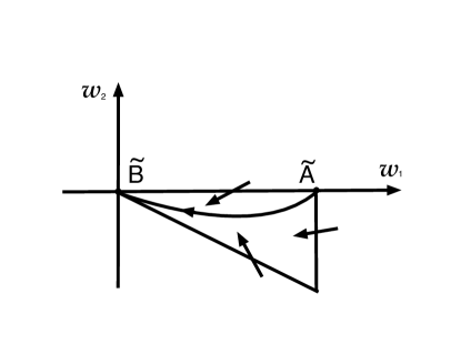
  Figure 1. Existence of a heteroclinic orbit for(3.2) by means of a trapping region argument.

It is known [25, 5, 6] that for $c\geq 2\sqrt{f^{\prime}(0)}=2\sqrt{\frac{1-\alpha}{\eta+1}}$, a monotone in $w_{1}$ asymptotic connection between the equilibria exists.

The classical proof of this fact is based on a construction of a trapping region in $(w_{1},w_{2})$-space for solutions of (3.2). In our case, the trapping region (see Fig. 1) is bounded by a triangle that consists of a segment of the $w_{1}$-axis between $(0,0)$ and $(1-\alpha^{2},0)$, a segment of the vertical line and a segment along line $w_{2}=-bw_{1}$, where $b$ is a number described below. The vector field points inside that triangular region through the vertical and horizontal sides. Along the side $w_{2}=-bw_{1}$, for the slope of the vector field we have

$$\frac{dw_{2}}{dw_{1}}=\frac{-cw_{2}-\frac{w_{1}(\sqrt{1-w_{1}}-\alpha)}{\eta+\sqrt{1-w_{1}}}}{w_{2}}\big{|}_{w_{2}=-bw_{1}}=\frac{cbw_{1}-\frac{w_{1}(\sqrt{1-w_{1}}-\alpha)}{\eta+\sqrt{1-w_{1}}}}{-bw_{1}}=-c+\frac{(\sqrt{1-w_{1}}-\alpha)}{b(\eta+\sqrt{1-w_{1}})}.$$

Since the function $\frac{s-\alpha}{\eta+s}$ is increasing, then over the interval $[\alpha,1]$ its maximum value is $\frac{1-\alpha}{\eta+1}$, so

$$\frac{dw_{2}}{dw_{1}}\leq-c+\frac{(1-\alpha)}{b(\eta+1)}.$$

If $c>2\sqrt{\frac{1-\alpha}{\eta+1}}$ and $b$ is a number strictly between $\frac{1}{2}\big{(}c\pm\sqrt{c^{2}-\frac{4(1-\alpha)}{\eta+1}}\big{)}$ then $c+\frac{(1-\alpha)}{b(\eta+1)}<-b$ and, therefore, $\frac{dw_{2}}{dw_{1}}<-b$. Thus, the vector field points inside the triangular region. If $c=2\sqrt{\frac{1-\alpha}{\eta+1}}$ and $b=\frac{c}{2}$, then $\frac{dw_{2}}{dw_{1}}\leq-b,$ so the vector field is aligned with the side $w_{2}=-bw_{1}$ and therefore the solution that starts inside of the triangle cannot leave either. Since the unstable manifold of $(1-\alpha^{2},0)$ points into this triangular region and the orbits are monotone in $w_{1}$ component, then the trajectory that follows the unstable manifold asymptotically connects to $(0,0)$.  

Next we show that this limiting orbit persists for sufficiently small $\delta>0$, and, then we argue that for every such $\delta$, there exists a sufficiently small $\epsilon>0$ such that the orbit persists in the full system (3.2).

By the dimension counting, in the two-dimensional phase space, the one-dimensional unstable manifold of $(1-\alpha^{2},0)$ and the two-dimensional stable manifold of $(0,0)$ intersect transversally. In the three-dimensional dynamical system (3.2) with sufficiently small $\delta>0$ the equilibrium $(1,0,0)$ has a two-dimensional stable manifold and a one-dimensional unstable manifold. Since $M_{\epsilon=0,\delta}$ is repelling, any solution of (3.2) approaching $(1,0,0)$ does so along $M_{\epsilon=0,\delta}$ and must entirely belong to it. On the other hand, the equilibrium $(\alpha,1-\alpha^{2},0)$ has a two-dimensional unstable manifold and a one-dimensional stable manifold. Moreover, this two-dimensional unstable manifold includes a direction transversal to $M_{\epsilon=0,\delta}$. Therefore the intersection of the two-dimensional unstable manifold of $(\alpha,1-\alpha^{2},0)$ with $M_{\epsilon=0,\delta}$ and thus with the two-dimensional stable manifold of $(1,0,0)$ is transversal. This intersection forms a heteroclinic orbit for (3.2) with sufficiently small $\delta>0$. We have the following lemma.

Lemma 3.

For every fixed $0<\alpha<1$, $\eta>0$, and $c>2\sqrt{\frac{1-\alpha}{\eta+1}}$, there is $\delta_{0}=\delta_{0}(\alpha,\eta,c)>0$ such that for any $0<\delta<\delta_{0}$ there exists a heteroclinic orbit of system (3.2) (equivalently, (3.2)) that asymptotically connects the saddle $(u_{1},w_{1},w_{2})=(\alpha,1-\alpha^{2},0)$ at $-\infty$ to the saddle $(1,0,0)$ at $+\infty$.

Next we consider (3.2) or equivalently (3.2). In the limit $\epsilon\to 0$, the analysis of the flow on $M_{\epsilon=0}$ resulted in Lemma 3. The equilibria $(\alpha,1-\alpha^{2},0)$ and $(1,0,0)$ from (3.2) lie on $M_{\epsilon=0}$ and they are also equilibria of the perturbed flow generated by (3.2) on the set $M_{\epsilon}$.

For sufficiently small $\epsilon$ the nature of equilibria is the same, one of them is still a saddle and the other is still a stable node. Since $M_{\epsilon}$ is attracting, the unstable manifold of the saddle $(\alpha,0,1-\alpha^{2},0)$ in (3.2) or (3.2) stays on $M_{\epsilon}$ as $\zeta$ changes from $-\infty$ to $+\infty$. Therefore the orbit is formed by the intersection of the unstable manifold of the saddle $(\alpha,0,1-\alpha^{2},0)$ and the stable manifold of the saddle $(1,0,0,0)$. This intersection persists since the intersection of the limits of involved invariant sets within $M_{\epsilon=0}$ is transversal and and entirely belongs to $M_{\epsilon}$. This argument proves the following theorem.

Theorem 4.

For every fixed $0<\alpha<1$, $\eta>0$, and $c>2\sqrt{\frac{1-\alpha}{\eta+1}}$, there exists $\delta_{0}=\delta_{0}(\alpha,\eta,c)>0$ such that for every $0<\delta<\delta_{0}$ there exists $\epsilon_{0}(\alpha,\eta,c,\delta)>0$ such that for each $0<\epsilon<\epsilon_{0}$ there is a heteroclinic orbit of system (3.2) (equivalently, (3.2)) that asymptotically connects the saddle $(u_{1},u_{2},w_{1},w_{2})=(\alpha,0,1-\alpha^{2},0)$ at $-\infty$ to the saddle $(u_{1},u_{2},w_{1},w_{2})=(1,0,0,0)$ at $+\infty$.

The dynamical system representation of a traveling front solution of a partial differential equation is a heteroclinic orbit, therefore for the system of partial differential equations (3.1) this theorem implies Theorem 1.

Remark. Both $u_{1}$ and $w_{1}$ components of the constructed limiting heteroclinic orbit of (3.2) are positive. It follows from the construction, that for sufficiently small $\delta$ and $\epsilon$, both $u_{1}$ and $w_{1}$ components of heteroclinic orbit of the system (3.2) are also positive.

4. Vanishing diffusion limit

4.1. Scaling and parameter regimes

In this section, we introduce a different scaling for the system (2.2) to analyze Cases 2, 3 and 4.

To describe Cases 2 and 3, we set $t=\delta\tau$ and $x=\sqrt{\delta}y$ in (2.2) to obtain

$$u_{\tau} = \epsilon_{u}u_{yy}+u\left(1-u\right)-\frac{uw}{1+u},$$

(30) $$w_{\tau} = \epsilon_{w}w_{yy}+\delta\frac{w\left(u-\alpha\right)}{\eta+u}.$$

In the co-moving coordinate frame $z=y-c\tau$, the system (4.1) reads

$$u_{\tau} = \epsilon_{u}u_{zz}+cu_{z}+u\left(1-u\right)-\frac{uw}{1+u},$$

(31) $$w_{\tau} = \epsilon_{w}w_{zz}+cw_{z}+\delta\frac{w\left(u-\alpha\right)}{\eta+u}.$$

Furthermore, we set $\zeta=z/c$, which effectively leads to a reduction in the number of parameters,

$$u_{\tau} = \frac{\epsilon_{u}}{c^{2}}u_{\zeta\zeta}+u_{\zeta}+u\left(1-u\right)-\frac{uw}{1+u},$$

(32) $$w_{\tau} = \frac{\epsilon_{w}}{c^{2}}\,w_{\zeta\zeta}+w_{\zeta}+\frac{\delta w\left(u-\alpha\right)}{\eta+u}.$$

We assume that $\epsilon_{u}$ and $\epsilon_{w}$ are positive and set $\epsilon={\epsilon_{u}}/{c^{2}}$ and $\mu={\epsilon_{w}}/{\epsilon_{u}}$. Clearly, $\mu>0$ and from the assumption $c>0$ it follows that $\epsilon>0$. The system (4.1) becomes

$$u_{\tau} = \epsilon u_{\zeta\zeta}+u_{\zeta}+u\left(1-u\right)-\frac{uw}{1+u},$$

(33) $$w_{\tau} = \epsilon\mu\,w_{\zeta\zeta}+w_{\zeta}+\frac{\delta w\left(u-\alpha\right)}{\eta+u}.$$

The corresponding traveling wave ode system then reads

$$0 = \epsilon u_{\zeta\zeta}+u_{\zeta}+u\left(1-u\right)-\frac{uw}{1+u},$$

(34) $$0 = \epsilon\mu\,w_{\zeta\zeta}+w_{\zeta}+\frac{\delta w\left(u-\alpha\right)}{\eta+u}.$$

We assume that $0<\epsilon\ll 1$ or, in other words, that the diffusion coefficient $\epsilon_{u}$ is small relative to the wave velocity $c$. This assumption is satisfied for any fixed $c$ when $\epsilon_{u}$ is sufficiently small or for for any fixed $\epsilon_{u}$ when $c$ is sufficiently large, thus the system (4.1) represents the traveling wave system for both Cases 2 and 3.

On the other hand, to describe Case 4, it is enough to rescale $t=\delta\tau$ and $x=\sqrt{\delta}\sqrt{d}\,y$ in (2.2), assuming that the characteristic length $d>0$ of the spatial variable $\sqrt{\delta}y$ is very large [30]. Indeed, then

$$u_{\tau} = \frac{\epsilon_{u}}{d}u_{yy}+u\left(1-u\right)-\frac{uw}{1+u},$$

(35) $$w_{\tau} = \frac{\epsilon_{v}}{d}w_{yy}+\delta\frac{w\left(u-\alpha\right)}{\eta+u}.$$

In the co-moving frame $z=y-ct$, (4.1) is

$$u_{\tau} = \frac{\epsilon_{u}}{d}u_{zz}+cu_{z}+u\left(1-u\right)-\frac{uw}{1+u},$$

(36) $$w_{\tau} = \frac{\epsilon_{v}}{d}w_{zz}+cw_{z}+\delta\frac{w\left(u-\alpha\right)}{\eta+u}.$$

If we further set $\zeta=z/c$ and $\epsilon={\epsilon_{u}}/{dc^{2}}$ and $\mu=\epsilon_{w}/\epsilon_{u}$, we obtain a system that looks exactly like (4.1). In the rest of this section we prove the following result.

Theorem 5.

For every fixed $0<\alpha<1$ and $\eta>0$ and $c\neq 0$, there exists $\delta_{0}=\delta_{0}(\alpha,\eta,c)>0$ such that for every $\delta\in(0,\delta_{0})$ there exists $\epsilon_{0}(\alpha,\eta,\delta)>0$ such that for each $0<\epsilon<\epsilon_{0}$ there is a translationally invariant family of fronts of the system (4.1), moving with speed $c$, which asymptotically connect the equilibrium $A=(\alpha,1-\alpha^{2})$ at $-\infty$ to the equilibrium $B=(1,0)$ at $+\infty$.

We assume $c>0$ without loss of generality, since if a traveling wave is found for $c>0$ then a coordinate change $\tau\to-\tau$ and $\zeta\to-\zeta$ captures traveling waves with negative velocity.

4.2. Traveling wave analysis.

In the coordinates $u_{1}=u$, $u_{2}=u_{\zeta}$, $w_{1}=w$, $w_{2}=w_{\zeta}$, (4.1) can be written as the following system of first order ordinary differential equations:

$$\frac{du_{1}}{d\zeta} = u_{2},$$

$$\epsilon\frac{du_{2}}{d\zeta} = -u_{2}-u_{1}(1-u_{1})+\frac{u_{1}w_{1}}{1+u_{1}},$$

$$\frac{dw_{1}}{d\zeta} = w_{2},$$

(37) $$\epsilon\frac{dw_{2}}{d\zeta} = -\frac{1}{\mu}w_{2}-\frac{\delta}{\mu}\frac{w_{1}\left(u_{1}-\alpha\right)}{\eta+u_{1}}.$$

We use geometric singular perturbation theory [15, 24, 26] to analyze (4.2). We consider (4.2) together with the following system obtained from (4.2) by rescaling the independent variable as $\zeta=\epsilon\xi$,

$$\frac{du_{1}}{d\xi} = \epsilon u_{2},$$

$$\frac{du_{2}}{d\xi} = -u_{2}-u_{1}(1-u_{1})+\frac{u_{1}w_{1}}{1+u_{1}},$$

$$\ \frac{dw_{1}}{d\xi} = \epsilon w_{2},$$

(38) $$\frac{dw_{2}}{d\xi} = -\frac{1}{\mu}w_{2}-\frac{\delta}{\mu}\frac{w_{1}\left(u_{1}-\alpha\right)}{\eta+u_{1}}.$$

The geometric singular perturbation theory allows us to extend the information obtained from the systems (4.2) and (4.2) when $\epsilon=0$ to the case of nonzero but sufficiently small $\epsilon>0$. We set $\epsilon=0$ in (4.2), thus obtaining an algebraic description of a set $M_{\epsilon=0}$ to which solutions of the limiting system belong

(39) $$M_{\epsilon=0}=\left\{(u_{1},u_{2},w_{1},w_{2}):\,u_{1}\geq 0,\,\,u_{2}=-u_{1}(1-u_{1})+\frac{u_{1}w_{1}}{1+u_{1}},\,\,w_{1}\geq 0,\,\,w_{2}=-\delta\frac{w_{1}\left(u_{1}-\alpha\right)}{\eta+u_{1}}\right\}$$

and the system of equation defined on $M_{\epsilon=0}$ which the solutions of the limiting system must satisfy

$$\frac{du_{1}}{d\zeta} = \frac{u_{1}w_{1}}{1+u_{1}}-u_{1}(1-u_{1}),$$

(40) $$\frac{dw_{1}}{d\zeta} = \delta\frac{w_{1}\left(\alpha-u_{1}\right)}{\eta+u_{1}}.$$

The set $M_{\epsilon=0}$ can be also described as the set of equilibrium points for the limiting system (4.2) with $\epsilon=0$,

$$\frac{du_{1}}{d\xi} = 0,$$

$$\frac{du_{2}}{d\xi} = -u_{2}-u_{1}(1-u_{1})+\frac{u_{1}w_{1}}{1+u_{1}},$$

$$\ \frac{dw_{1}}{d\xi} = 0,$$

(41) $$\frac{dw_{2}}{d\xi} = -\frac{1}{\mu}w_{2}-\frac{\delta}{\mu}\frac{w_{1}\left(u_{1}-\alpha\right)}{\eta+u_{1}}.$$

It is easy to see that the two-dimensional set $M_{\epsilon=0}$ is normally hyperbolic and attracting. Indeed, besides the two zero eigenvalues, each point of $M_{\epsilon=0}$ has eigenvalues $-1$ and $-\frac{1}{\mu}$. Fenichel’s invariant manifold theory [15, 24] implies that $M_{\epsilon=0}$ perturbs to an invariant set $M_{\epsilon}$ for the full system, if $\epsilon$ is sufficiently small. $M_{\epsilon}$ is an $\epsilon$-order perturbation of $M_{\epsilon=0}$ and the flow on $M_{\epsilon}$ is

$$\frac{du_{1}}{d\zeta} = \frac{u_{1}w_{1}}{1+u_{1}}-u_{1}(1-u_{1})+O(\epsilon),$$

(42) $$\frac{dw_{1}}{d\zeta} = \delta\frac{w_{1}\left(\alpha-u_{1}\right)}{\eta+u_{1}}+O(\epsilon).$$

Let

$$f_{1}=\frac{u_{1}w_{1}}{1+u_{1}}-u_{1}(1-u_{1}),\quad f_{2}=\frac{w_{1}\left(\alpha-u_{1}\right)}{\eta+u_{1}}.$$

The eigenvalues of the linearization of (4.2) at an equilibrium are given by

(43) $$\lambda_{1,2}=\frac{1}{2}\left(\delta f_{2w_{1}}+f_{1u_{1}}\pm\sqrt{(\delta f_{2w_{1}}+f_{1u_{1}})^{2}-4\delta(f_{1u_{1}}f_{2w_{1}}-f_{1w_{1}}f_{2u_{1}})}\right),$$

where $f_{1}$ and $f_{2}$ and their derivatives are evaluated at the equilibrium. The derivatives of functions $f_{1}$ and $f_{2}$ are

(44) $$\quad f_{1u_{1}}=\frac{w_{1}}{(1+u_{1})^{2}}-1+2u_{1},\quad f_{1w_{1}}=\frac{u_{1}}{u_{1}+1},\quad f_{2u_{1}}=-\frac{w_{1}(\eta+\alpha)}{(\eta+u_{1})^{2}},\quad f_{2w_{1}}=\frac{\alpha-u_{1}}{\eta+u_{1}}.$$

At the equilibrium $A$

(45) $$f_{1u_{1}}(A)=\frac{2\alpha^{2}}{1+\alpha},\quad f_{1w_{1}}(A)=\frac{\alpha}{1+\alpha},\quad f_{2u_{1}}(A)=-\frac{1-\alpha^{2}}{\eta+\alpha},\quad f_{2w_{1}}(A)=0.$$

Since $f_{2w_{1}}(A)=0$, the eigenvalues (43) of the linearization of (4.2) at the equilibrium $A$ are

(46) $$\lambda_{1,2}(A)=\frac{1}{2}\left(f_{1u_{1}}(A)\pm\sqrt{f_{1u_{1}}^{2}(A)+4\delta f_{1w_{1}}(A)f_{2u_{1}}(A)}\right).$$

Since $f_{1u_{1}}(A)>0$, the eigenvalues $\lambda_{1,2}(A)$ are positive when $\delta\in(0,\delta_{0})$, where

(47) $$\delta_{0}=-\frac{f_{1u_{1}}^{2}(A)}{4f_{1w_{1}}(A)f_{2u_{1}}(A)}=\frac{\alpha^{3}(\eta+\alpha)}{(1-\alpha)(1+\alpha)^{2}}.$$

Therefore, when $\delta\in(0,\delta_{0})$, the equilibrium $A$ is an unstable node.

The eigenvalues of the linearization at the equilibrium $B=(1,0)$ are

(48) $$\lambda_{1}(B)=1,\quad\lambda_{2}(B)=-\delta\frac{1-\alpha}{\eta+\alpha},$$

therefore, when $0<\alpha<1$, the equilibrium $B$ is a saddle.

4.3. Singular front at $\delta=0$

We are interested in proving the existence of heteroclinic orbits of the system (4.2). We do that by exploiting the slow-fast structure of (4.2) with regards to $\delta$ when $\delta$ is small.

Rescaling $\varsigma=\zeta/\delta$, we obtain the fast system

$$\delta\frac{du_{1}}{d\varsigma} = \frac{u_{1}w_{1}}{1+u_{1}}-u_{1}(1-u_{1}),$$

(49) $$\frac{dw_{1}}{d\varsigma} = \frac{w_{1}\left(\alpha-u_{1}\right)}{\eta+u_{1}}.$$

When $\delta=0$, the system (4.2) reads

$$\frac{du_{1}}{d\zeta} = \frac{u_{1}w_{1}}{1+u_{1}}-u_{1}(1-u_{1}),$$

(50) $$\frac{dw_{1}}{d\zeta} = 0,$$

and the system (4.3) reads

$$0 = \frac{u_{1}w_{1}}{1+u_{1}}-u_{1}(1-u_{1}),$$

(51) $$\frac{dw_{1}}{d\varsigma} = \frac{w_{1}\left(\alpha-u_{1}\right)}{\eta+u_{1}}.$$

The system (4.3) has the set of equilibria which is also the critical manifold for (4.3) described in (25), but, again, only one curve out of this set is relevant

$$M_{\epsilon=0,\,\delta=0}=\{(u_{1},w_{1}):u_{1}=\sqrt{1-w_{1}},\,w_{1}<1\},$$

The set $M_{\epsilon=0,\,\delta=0}$ is a part of the right branch of the parabola $w_{1}=1-u_{1}^{2}$. The branch of the parabola with negative $u_{1}$, as well as the set with $u_{1}=0$ do not contain the equilibria that we are interested in.

The linearization of (4.2) around $M_{\epsilon=0,\,\delta=0}$ has an eigenvalue $\frac{2(1-w_{1})}{1-\sqrt{1-w_{1}}}$, therefore $M_{\epsilon=0,\,\delta=0}$ is a normally hyperbolic, repelling manifold with respect to the flow of (4.2). On $M_{\epsilon=0,\,\delta=0}$ the solutions the system (4.3) satisfy

(52) $$\frac{dw_{1}}{d\varsigma}=w_{1}\frac{\alpha-\sqrt{1-w_{1}}}{\eta+\sqrt{1-w_{1}}},$$

the dynamics of which is easy to understand. Indeed, the two equilibria of the equation (52) are $w_{1}=0$ and $w_{1}=1-\alpha^{2}$: $w_{1}=0$ (which corresponds to $B$) is stable and $w_{1}=1-\alpha^{2}$ (which corresponds to $A$) is unstable (Fig. 2).

$\begin{array}[]{lclc}\includegraphics[width=238.49121pt]{p2.pdf}&\includegraphics[width=238.49121pt]{p3.pdf}\end{array}$

Figure 2. The dynamics of (4.2). Left panel: singular solution, $\delta=0$. Right panel: perturbed solution, $0<\delta\ll 1$.

Since $M_{\epsilon=0,\,\delta=0}$ is normally hyperbolic, it persists as an invariant set $M_{\epsilon=0,\,\delta}$ for (4.2) when $\delta$ is sufficiently small. On $M_{\epsilon=0,\,\delta}$, the flow is a $\delta$-order perturbation of the flow described in (52). Within the two-dimensional system (4.3), the equilibrium $A$ has a two dimensional unstable manifold and the equilibrium $B$ has a one dimensional stable manifold. By dimension counting their intersection is transversal, so it persists when a sufficiently small $\delta>0$ is introduced, therefore the following lemma holds. The persistence of the limiting orbit that corresponds to $\delta=0$ also follows from the general result [19, Corollary 3.3] which encapsulates the “transversality through a dimension counting” argument. Therefore the following lemma holds.

Lemma 6.

For every fixed $0<\alpha<1$ and $\eta>0$, there is $\delta_{0}=\delta_{0}(\alpha,\eta)>0$ such that for any $0<\delta<\delta_{0}$ there exists a heteroclinic orbit of system (4.3) that asymptotically connects the saddle $(u_{1},w_{1},w_{2})=(\alpha,1-\alpha^{2},0)$ at $-\infty$ to the saddle $(1,0,0)$ at $+\infty$.

This lemma proves that the singular limit of (4.2) as $\epsilon\to 0$ has a heteroclinic connection on the slow manifold $M_{\epsilon=0}$ (see (39)).

Since $M_{\epsilon=0}$ is normally hyperbolic and attracting it persists as an invariant manifold $M_{\epsilon}$ for the system (4.2) (equivalently, (4.2)).

For sufficiently small $\epsilon>0$, $M_{\epsilon}$ is attracting, therefore the unstable manifold of the saddle $(1,0,0,0)$ stays on $M_{\epsilon}$ for all $\xi$. Therefore any orbit that originates at $(1,0,0,0)$ lays on a two-dimensional set $M_{\epsilon}$, so the unstable manifold of $(1,0,0,0)$ and the stable manifold of $(\alpha,0,1-\alpha^{2},0)$ still intersect as their limits as $\epsilon\to 0$ intersect transversally within $M_{\epsilon=0}$. The following theorem then holds.

Theorem 7.

For every fixed $0<\alpha<1$ and $\eta>0$ there exists $\delta_{0}=\delta_{0}(\alpha,\eta)>0$ such that for every $0<\delta<\delta_{0}$ there exists $\epsilon_{0}(\alpha,\eta,\delta)>0$ such that for each $0<\epsilon<\epsilon_{0}$ there is a heteroclinic orbit of the system (4.2), or, equivalently, of the system (4.2)) that asymptotically connects the saddle $(u_{1},u_{2},w_{1},w_{2})=(\alpha,0,1-\alpha^{2},0)$ at $-\infty$ to the saddle $(u_{1},u_{2},w_{1},w_{2})=(1,0,0,0)$ at $+\infty$.

5. The influence of the assumption $\gamma=1$.

The spatially homogeneous equilibria of the PDE (2.2) are

(53) $$A=(\alpha,(\gamma-\alpha)(1+\alpha)),\,\,\,\,B=(\gamma,0),\,\,\,\,O=(0,0).$$

When $\gamma\geq\alpha$, all of these equilibria have nonnegative components and therefore are relevant for population modeling.

In the limiting systems (3.2) and (4.2), the co-existence equilibrium with positive components corresponds to the equilibrium $A$. It is given by the intersection of the parabolic nullcline $w=(1+u)(\gamma-u)$ and the verical nullcline $u=\alpha$. We observe that the dynamics near the equilibrium depends on where the equilibrium is located relative to the vertex $V=(\frac{\gamma-1}{2},\frac{(\gamma+1)^{2}}{4})$ of the parabolic nullcline. When the parameters are in the region $\{(\alpha,\gamma):0<\gamma<1,\,\,\,0<\alpha<\gamma\}$ the equilibrium $A$ is in the open first quadrant of $uw$-plane and is strictly to the right of the vertex $V$. In this situation, the proof and the results described in Theorems  1 and 5 hold. The assumption $\gamma=1$ means that the vertex $V=(0,1)$ is on the vertical axis and $0<\alpha<1$ guarantees that the equilibrium $A$ which is now $(\alpha,1-\alpha^{2})$ to the right of the parabola’s vertex. In the parameter region $\{(\alpha,\gamma):\gamma\geq 1,\,\,\,\frac{\gamma-1}{2}<\alpha<\gamma\}$ the results still hold, although some minor, technical changes in the proofs are required.

6. Holling-Tanner model

The importance of the Fisher-KPP dynamics in a system has been studied before. In paper [11], Ducrot considers a diffusive predator-prey model

$$U_{\tau} = \epsilon_{u}U_{XX}+AU(1-\frac{U}{\mathcal{K}})-\frac{\mathcal{B}UW}{\mathcal{E}+U},$$

(54) $$W_{\tau} = \epsilon_{w}W_{XX}+\mathcal{R}W\left(1-\frac{\mathcal{H}W}{U}\right),$$

where $t>0$ is the time and $x$ is the spacial variable, $U$ represents the density of the prey, and $V$ is the density of the predator. The parameters $\alpha$, $\delta$, $\beta$, and the diffusion coefficients $\epsilon_{u}$ and $\epsilon_{w}$ are positive. The system (6) is obtained by adding diffusion terms to an ode system for Holling-Tanner predator-prey model [4, 23, 28, 29, 30, 32, 37, 39] where the predation rate is known as Holling type II functional response $\frac{U}{\mathcal{E}+U}$ [22].

The model (6) has been extensively studied. For example, transition fronts have been investigated numerically in [38], the existence of fronts in vanishing diffusion limit has been proved in [21], the existence of fronts for more general type of nonlinearities was proved in [1] in a parameter regime that does not capture the situation considered in this paper. A result relevant to our work on Rosenzweig-MacArthur system is the result from [11] where, in the most general case of a multi-dimensional spacial variable $x\in\mathbb{R}^{n}$, Ducrot investigates the spreading speed of the small perturbations to the co-existence equilibrium which is the equilibrium with positive values for both predator and prey densities. The author shows in [11] that if initially the predator is introduced in a compactly supported manner, while the prey is initially uniformly well distributed, then the spreading speed of the perturbations is defined by the spreading speed in the associated Fisher-KPP scalar equation.

In this section we consider (6) with $x\in\mathbb{R}$ in a specific parameter regime and construct fronts which are small perturbations of the fronts in scalar Fisher-KPP equation in a way similar to one used in Section 3. We spare readers the repetition of the details and present only a brief overview of the analysis.

We consider a new scaling of the system (6), given by

$$\begin{array}[]{llll}u=\frac{U}{\mathcal{E}},&w=\frac{\mathcal{K}\mathcal{B}}{\mathcal{E}^{2}\mathcal{A}}W,&x=\sqrt{\frac{\mathcal{R}}{\epsilon_{w}}}X,&\quad t=\mathcal{R}\tau,\\ \gamma=\frac{\mathcal{K}}{\mathcal{E}},&\delta=\frac{\mathcal{K}\mathcal{R}}{\mathcal{E}\mathcal{A}},&\quad\beta=\frac{\mathcal{A}\mathcal{H}\mathcal{E}}{\mathcal{B}\mathcal{K}},&\quad\epsilon=\frac{\epsilon_{u}}{\epsilon_{w}}.\end{array}$$

In these new variables the system (6) reads

$$u_{t} = \epsilon u_{xx}+\frac{1}{\delta}\left(u(\gamma-u)-\frac{uw}{1+u}\right),$$

(55) $$w_{t} = w_{xx}+w\left(1-\frac{\beta w}{u}\right).$$

For the computational brevity we will set $\gamma=1$. We are interested in front solutions asymptotically connecting $(u,w)=(1,0)$ and $(u,w)=\left(\frac{-1+\sqrt{4\beta^{2}+1}}{2\beta},\frac{-1+\sqrt{4\beta^{2}+1}}{2\beta^{2}}\right)$. Switching to the moving frame $z=x-ct$ in (6), we obtain

$$u_{t} = \epsilon u_{zz}+cu_{z}+\frac{1}{\delta}\left(u(1-u)-\frac{uw}{1+u}\right),$$

(56) $$w_{t} = w_{zz}+cw_{z}+w\left(1-\frac{\beta w}{u}\right).$$

The fronts in the system (6) are associated with heteroclinic orbits of the dynamical system

$$u_{1}^{\prime} = u_{2},$$

$$\epsilon u_{2}^{\prime} = -cu_{2}-\frac{1}{\delta}\left(u_{1}(1-u_{1})-\frac{u_{1}w_{1}}{1+u_{1}}\right),$$

$$w_{1}^{\prime} = w_{2},$$

(57) $$w_{2}^{\prime} = -cw_{2}-w_{1}\left(1-\frac{\beta w_{1}}{u_{1}}\right),$$

where $u_{1}=u$, $w_{1}=w$, and the derivative is taken with respect to $z$. Assuming that $0<\epsilon\ll\delta\ll 1$, and following the same multiple scale reduction as in Section 3, we obtain that the limiting behavior is defined by the dynamical system

$$w_{1}^{\prime} = w_{2},$$

(58) $$w_{2}^{\prime} = -cw_{2}-w_{1}\frac{\sqrt{1-w_{1}}-\beta w_{1}}{\sqrt{1-w_{1}}},$$

which is related to the traveling wave equation in a scalar Fisher-KPP equation

(59) $$w_{t}=w^{\prime\prime}+cw^{\prime}+w\frac{\sqrt{1-w}-\beta w}{\sqrt{1-w}}$$

Thus, a theorem holds that is similar to Theorem 4 for the slowly diffusing prey case for Rosenzweig-MacArthur system:

Theorem 8.

For every fixed $\beta>0$ and $c>2$, there exists $\delta_{0}=\delta_{0}(\beta)>0$ such that for every $0<\delta<\delta_{0}$ there exists $\epsilon_{0}(\beta)>0$ such that for each $0<\epsilon<\epsilon_{0}$ there is a heteroclinic orbit of system (6) that asymptotically connects the saddle $(u_{1},u_{2},w_{1},w_{2})=(\frac{-1+\sqrt{4\beta^{2}+1}}{2\beta},0,\frac{-1+\sqrt{4\beta^{2}+1}}{2\beta^{2}},0)$ at $-\infty$ to the saddle $(u_{1},u_{2},w_{1},w_{2})=(1,0,0,0)$ at $+\infty$.

The latter implies an analogue of Theorem 1 for the diffusive Holling-Tanner model (6):

Theorem 9.

For every fixed $\beta>0$ and $c>2$, there exists $\delta_{0}=\delta_{0}(\beta)>0$ such that for every $0<\delta<\delta_{0}$ there exists $\epsilon_{0}(\beta)>0$ such that for each $0<\epsilon<\epsilon_{0}$ there is a translationally invariant family of fronts of the system (6) moving with speed $c$ that asymptotically connect the equilibrium $(u,w)=(\frac{-1+\sqrt{4\beta^{2}+1}}{2\beta},\frac{-1+\sqrt{4\beta^{2}+1}}{2\beta^{2}})$ at $-\infty$ to the equilibrium $(u,w)=(1,0)$ at $+\infty$.

For the diffusive Holling-Tanner model (6) the case of vanishing diffusion limit when both $\epsilon_{u}$ and $\epsilon_{w}$ are very small is considered in [21] and the existence of fronts is analytically proved. As in the case of the vanishing diffusion limit for Rosenzweig-MacArthur system, the connection of these fronts with Fisher-KPP fronts is not directly observed, as opposed to the regime described above.

7. Acknowledgements and other remarks.

During the work on this project, Ghazaryan was supported by the NSF grant DMS-1311313, and Manukian was supported by the Simons Foundation through the Collaboration grant #246535. Hong Cai worked on this project as a student at Miami University and later as a student at Brown University.

The authors thank the anonymous reviewers for the detailed feedback and constructive recommendations.

References

• [1] S. Ai, Y. Du, and R. Peng. Traveling waves for a generalized Holling-Tanner predator-prey model. J. Differential Equations 263 (2017) 7782-7814.
• [2] E. Almanza-Vasquez, E. González-Olivares, and B. González-Yanez. Dynamics of Lotka-Volterra predator-prey model considering saturated refuge for prey. BIOMAT 2011 International Symposium on Mathematical and Computational Biology, World Scientific Co. Pte. Ltd., Singapore, 2012, 62–72.
• [3] E. Almanza-Vasquez, R.-D. Ortiz-Ortiz, and A.-M. Marin-Ramirez. Bifurcations in the dynamics of Rosenzweig-MacArthur predator-prey model considering saturated refuge for the preys. Applied Mathematical Sciences 9 (2015) 7475–7482.
• [4] C.  Arancibia-Ibarra, J.. Flores, M. Bode, G. J. Pettet, P. van Heijster. A May-Holling-Tanner predator-prey model with multiple Allee effects on the prey and an alternative food source for the predator. Preprint: arXiv:1904.02886v2 .
• [5] D. G. Aronson and H. F. Weinberger. Nonlinear diffusion in population genetics, combustion, and nerve pulse propagation. Partial differential equations and related topics (Program, Tulane Univ., New Orleans, La., 1974), Lecture Notes in Math., Vol. 446, Springer, Berlin, 1975, 5–49.
• [6] D. G. Aronson and H. F. Weinberger. Multidimensional nonlinear diffusion arising in population genetics. Adv. in Math. 30 (1978) 33–76.
• [7] M. A. Aziz-Alaoui and M. Daher Okiye. Boundedness and global stability for a predator-prey model with modified Leslie-Gower and Holling-type II schemes. Applied Mathematics Letters 16(2003) 1069–1075.
• [8] H. Berestycki, F. Hamel, A. Kiselev, and L. Ryzhik. Quenching and propagation in KPP reaction-diffusion equations with a heat loss. Arch. Ration. Mech. Anal. 178 (2005) 57–80.
• [9] P. T. Cardin and M. A. Teixeira. Fenichel theory for multiple time scale singular perturbation problems. SIAM J. Appl. Dyn. Syst. 16 (2017) 1425–1452.
• [10] A. S. Dagbovie and J. A. Sherratt. Absolute stability and dynamical stabilisation in predator-prey systems. J. Math. Biol. 68 (2014) 1403–1421.
• [11] A. Ducrot. Convergence to generalized transition waves for some Holling-Tanner prey-predator reaction-diffusion system. J. Math. Pures Appl. 100 (2013) 1–15.
• [12] S. Dunbar. Traveling waves in diffusive predator-prey equations: periodic orbits and point-to-periodic heteroclinic orbits. SIAM J. on Applied Mathematics 86 (1986) 1057–1078.
• [13] I. L. Hanski, L. Hansson, and H. Henttonen. Specialist predators, generalist predators and the microtine rodent cycle. J. Animal Ecology 60 (1991) 353–367.
• [14] J. Huang, G. Lu, and S. Ruan. Existence of traveling wave solutions in a diffusive predator-prey model. J. Math. Biol. 46 (2003) 132–152.
• [15] N. Fenichel. Geometric singular perturbation theory for ordinary differential equations. J. Differ. Equations 55 (1979) 763–783.
• [16] P. C. Fife. Mathematical Aspects of Reacting and Diffusing Systems. Springer, Berlin, 1977.
• [17] R. A. Fisher. The wave of advance of advantageous genes. Ann. Eugenics 7 (1937) 353–369.
• [18] S.-C. Fu and J.-C. Tsai. Wave propagation in predator-prey systems. Nonlinearity 28 (2015) 4389–4423.
• [19] I. Gasser and P. Szmolyan. A geometric singular perturbation analysis of detonation and deflagration waves. SIAM J. on Math. Analysis 24 (1993) 968–986.
• [20] A. Ghazaryan, V. Manukian. Coherent structures in a model for mussel-algae Interaction. SIAM J. of Dynamical Systems. 14 (2015) 893–913.
• [21] A. Ghazaryan, V. Manukian, and S. Schecter. Travelling waves in the Holling-Tanner model with weak diffusion. Proc. A. 471 (2177): 20150045, 16 pp.
• [22] C. S. Holling. The characteristics of simple types of predation and parasitism. Canadian Entomologist 91 (1959) 293–320.
• [23] S. B. Hsu and T.-W. Huang. Global stability for a class of predator-prey systems. SIAM J. Appl. Math. 31(1995) 53–98.
• [24] C. Jones. Geometric singular perturbation theory. In Dynamical Systems (Montecatini Terme, 1994), Lecture Notes in Math. Springer, Berlin. 1609(1995) 44–118.
• [25] A. Kolmogorov, I. Petrovskii, and N. Piskunov. A study of the diffusion equation with increase in the amount of substance, and its application to a biological problem. In V. M. Tikhomirov, editor, Selected Works of A. N. Kolmogorov I, pages 248-270. Kluwer 1991, ISBN 90-277-2796-1. Translated by V. M. Volosov from Bull. Moscow Univ., Math. Mech. 1(1937) 1–25.
• [26] C. Kuehn. Multiple Time Scale Dynamics. Springer, New York, 2015.
• [27] V. Manukian. On traveling waves of Gray-Scott model. Dynamical Systems: An International Journal 30 (2015) 270–296.
• [28] R. M. May. On relationships among various types of population models. American Naturalist 107 (1973) 46–57.
• [29] R. M. May. Stability and Complexity in Model Ecosystems. Princeton University Press, Princeton, NJ, 1974.
• [30] J. D. Murray. Mathematical Biology II: Spatial Models and Biomedical Applications. Springer, New York, 2003.
• [31] M. R. Owen and M. A. Lewis. How predation can slow, stop or reverse a prey invasion. Bull. Math. Biol. 63 (2001) 655–684.
• [32] E.  Renshaw. Modelling Biological Populations in Space and Time. Cambridge University Press, Cambridge, 1991.
• [33] M. L. Rosenzweig and R. H. MacArthur. Graphical Representation and Stability Conditions of Predator-Prey Interactions. The American Naturalist 97 (1963) 209–223.
• [34] E. Sáez and E.  González-Olivares. Dynamics of a predator-prey model. SIAM J. Appl. Math. 59 (1999) 1867–1878.
• [35] J. A. Sherratt and M. J. Smith. The effects of unequal diffusion coefficients on periodic travelling waves in oscillatory reaction-diffusion systems. Phys. D 236 (2007) 90–103.
• [36] J. A. Sherratt and M. J. Smith. Periodic travelling waves in cyclic populations: field studies and reaction-diffusion models. J. R. Soc. Interface 5 (2008) 483–505.
• [37] J. T. Tanner. The stability and the intrinsic growth rates of prey and predator populations. Ecology 56 (1975) 855–867.
• [38] R. K. Upadhyay, V. Volpert, and N. K. Thakur. Propagation of Turing patterns in a plankton model. J. Biol. Dyn. 6 (2012) 524–538.
• [39] V. Volpert and S. Petrovskii. Reaction-diffusion waves in biology. Phys. Life Rev. 6 (2009) 267–310.
• [40] A. I. Volpert, V. A. Volpert, and V. A. Volpert. Traveling Wave Solutions of Parabolic Systems. American Mathematical Society, Providence, 1994.