A Survey of Adaptive Resonance Theory Neural Network Models for Engineering Applications

Abstract

This survey samples from the ever-growing family of adaptive resonance theory (ART) neural network models used to perform the three primary machine learning modalities, namely, unsupervised, supervised and reinforcement learning. It comprises a representative list from classic to modern ART models, thereby painting a general picture of the architectures developed by researchers over the past 30 years. The learning dynamics of these ART models are briefly described, and their distinctive characteristics such as code representation, long-term memory and corresponding geometric interpretation are discussed. Useful engineering properties of ART (speed, configurability, explainability, parallelization and hardware implementation) are examined along with current challenges. Finally, a compilation of online software libraries is provided. It is expected that this overview will be helpful to new and seasoned ART researchers.

1 Introduction

Adaptive Resonance Theory (ART) [Grossberg, 1976a, b, 1980, 2013] is a biologically-plausible theory of how a brain learns to consciously attend, learn and recognize patterns in a constantly changing environment. The theory states that resonance regulates learning in neural networks with feedback (recurrence). Thus, it is more than a neural network architecture, or even a family of architectures. However, it has inspired many neural network architectures that have very attractive properties for applications in science and engineering, such as being fast and stable incremental learners with relatively small memory requirements and straightforward algorithms [Wunsch II, 2009]. In this context, fast learning refers to the ability of the neurons’ weight vectors to converge to their asymptotic values directly with each input sample presentation. These, and other properties, make ART networks attractive to many researchers and practitioners, as they have been used successfully in a variety of science and engineering applications.

ART addresses the problem of stability vs. plasticity [Grossberg, 1980, Carpenter & Grossberg, 1987a]. Plasticity refers the ability of a learning algorithm to adapt and learn new patterns. In many such learning systems plasticity can lead to instability, a situation in which learning new knowledge leads to the loss or corruption of previously-learned knowledge, also known as catastrophic forgetting. Stability, on the other hand, is defined by the condition that no prototype vector can take on a previous value after it has changed, and that an infinite presentation of inputs results in forming a finite number of clusters [Xu & Wunsch II, 2009, Moore, 1989]. ART addresses this stability-plasticity dilemma by introducing the ability to learn arbitrary input patterns in a fast and stable self-organizing fashion without suffering from catastrophic forgetting.

There have been some previous studies with similar objectives of surveying the ART neural network literature [Du, 2010, Amorim et al., 2011, Jain et al., 2014, RamaKrishna et al., 2014]. This survey expands on those works, compiling a broad and informative sampling of ART neural network architectures from the ever-growing machine learning literature. It captures a representative set of examples of various ART architectures in the unsupervised, supervised and reinforcement learning modalities, as well as some models that cross these boundaries and/or combine multiple learning modalities. The overarching goal of this survey is to provide researchers with an accessible coverage of these models, with a focus on their motivations, interpretations for engineering applications and a discussion of open problems for consideration. It is not meant as a comparative assessment of these models but rather a roadmap to assess options.

The remainder of this paper is organized as follows. Section 2 presents a sampling of unsupervised learning (UL) ART models, divided into elementary, topological, hierarchical, biclustering and data fusion architectures. Section 3 discusses supervised learning (SL) ART models for both classification and regression. Reinforcement learning (RL) ART models are discussed in Section 4. Sections 5 and 6 discuss some of the useful properties of ART architectures and open problems in this field, respectively. Section 7 provides links to some repositories of ART neural network code, and Section 8 concludes the paper.

2 ART models for unsupervised learning

2.1 Elementary architectures

At their core, the elementary ART models are predominantly used for unsupervised learning applications. However, they also lay the foundation to build complex ART-based systems capable of performing all three machine learning modalities (Secs. 2, 3, and 4). This section describes the main characteristics of ART family members in terms of their code representation, long-term memory unit, system dynamics (which encompasses activation, match, resonance and learning) and user-defined parameters. For clarity, Table 1 summarizes the common notation used in the following subsections.

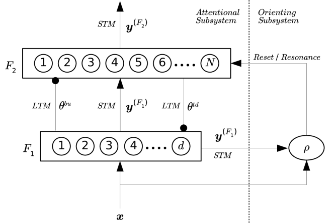
An elementary ART neural network model (Fig. 1) usually consists of two fully connected layers as well as a system responsible for its decision-making capabilities:

• Feature representation field F₁: this is the input layer. In feedforward mode, the output $\bm{y}^{(F_{1})}$ of this layer, or short-term memory (STM), simply propagates the input samples $\bm{x}\in\mathbb{R}^{d}$ to the F₂ layer via the bottom-up long-term memory units (LTMs) $\bm{\theta}^{bu}$. In feedback mode, the F₁ layer works as a comparator, in which $\bm{x}$ and the F₂’s expectation (in the form of a top-down LTM $\bm{\theta}^{td}$) are compared and the outcome $\bm{y}^{(F_{1})}$ is sent to the orienting subsystem. Hence, F₁ is also known as comparison layer.

• Category representation field F₂: this layer yields the network output $\bm{y}^{(F_{2})}$ (STM). It is also known as recognition or competitive layer. Neurons, prototypes, categories and templates will be used interchangeably when referring to the F₂ nodes. The LTM associated with a category $j$ is $\bm{\theta}_{j}=\{\bm{\theta}^{bu}_{j},\bm{\theta}^{td}_{j}\}$, $j=1,...,N$. Note that not all elementary ART models discussed in this survey have independent bottom-up and top-down LTM parts; however, $\bm{\theta}$ is always used to indicate the LTM (or set of adaptive parameters) of a given category.

• Orienting subsystem: this is a system that regulates both the search and learning mechanisms by inhibiting or allowing categories to resonate.

Figure 1: Elementary ART model underlying various designs. The orienting subsystem uses the vigilance threshold to regulate whether ART can go into resonance or if it must reset.

Table 1: Unsupervised ART models notation.

Notation Description $\bm{x}$ input sample ($\bm{x}\in\bm{X}$) $d$ original data dimensionality ($\bm{x}\in\mathbb{R}^{d}$) F₁ feature representation field F₂ category representation field $N$ number of categories $\bm{y}^{(F_{1})}$ F₁ activity/output (STM) $\bm{y}^{(F_{2})}$ F₂ activity/output (STM) $c$ a category $\bm{\theta}$ category parameters (LTM unit) $T$ activation function $M$ match function $J$ chosen category index (via WTA) $\rho$ vigilance parameter $VR$ vigilance region

Note that some ART models represent pre-processing procedures of the input samples by another layer preceding F₁, namely the Input field F₀. In this survey, it is assumed that the inputs to an ART network have already gone through the required transformations, and thus this layer is omitted from the discussion.

ART models are competitive, self-organizing, dynamic and modular networks. When a sample $\bm{x}$ is presented, a winner-takes-all (WTA) competition takes place over its categories at the output layer F₂. Then, the neuron $J$ that optimizes that model’s activation function across the nodes is chosen, e.g., the neuron that maximizes some similarity measure $T$ to the presented sample

$$J=\operatorname*{arg\,max}\limits_{j}(T_{j}).$$ (1)

A category represents a hypothesis. Therefore, a hypothesis test cycle, commonly referred to as a vigilance test, is performed by the orienting subsystem to determine the adequacy of the selected category, i.e., the winner category must satisfy a match criterion (or several match criteria). If the confidence on such a hypothesis is larger than the minimum threshold (namely, the vigilance parameter $\rho$), the neural network enters in a resonance state and learning (i.e., adaptation of the long-term memory (LTM) units) is allowed. Otherwise, category $J$ is inhibited, the next highest ranked category is selected, and the search resumes. If no category satisfies the required resonance condition(s), then a new one is created to encode the presented input sample. This ability to reject a hypothesis/category via a two-way similarity measure, i.e. permissive clustering [Seiffertt & Wunsch II, 2010], makes ART stand out from other methods, such as k-means [MacQueen, 1967]. A vigilance region ($VR$) for a given network category $j$ can be defined in the data space as

$$VR_{j}=\{\bm{x}:M_{j}(\bm{x})\mbox{ satisfies the resonance constraint}\},$$ (2)

where $M_{j}$ is the match function, which yields the confidence on hypothesis $j$. In other words, it is the region in the input space containing the set of all points such that the resonance criteria is met. Therefore satisfying (or not) the vigilance test for sample $\bm{x}$ can be modeled using

$$\mathds{1}_{VR_{j}}(\bm{x})=\begin{cases}1,&\mbox{if }\bm{x}\in VR_{j}\\ 0,&\mbox{otherwise}\end{cases},$$ (3)

where $\mathds{1}_{\{\cdot\}}$ is the indicator function.

The resonance constraint in Eq. (2) is depends on the vigilance parameter $\rho$, which regulates the granularity of the network as ART maps samples to categories. Particularly, lower vigilance encourages generalization [Vigdor & Lerner, 2007]. Selecting the vigilance parameter is a difficult task in clustering problems. Concretely, the problem of choosing the number of clusters is traded for the problem of choosing the vigilance value.

Distinct ART models feature specific LTM units, activation and match functions, vigilance criteria and learning laws. Algorithm 1 summarizes the dynamics of an elementary ART model.

Input : $\bm{x}$, $\{\bm{\alpha},\bm{\beta},\bm{\gamma},\bm{\rho},\bm{\lambda}\}$ (parameters).

Output : $\bm{y}^{(F_{2})}$.

 

/* Notation

$\mathcal{C}$: set of ART nodes.

$\Lambda$: subset of highly active nodes ($\Lambda\subseteq\mathcal{C}$).

$\bm{\theta}$: LTM unit.

$\bm{\alpha}$: activation function parameter(s).

$\bm{\beta}$: learning function parameter(s).

$\bm{\gamma}$: match function parameter(s).

$\bm{\rho}$: vigilance parameter(s).

$\bm{\lambda}$: initialization parameter(s).

$f_{T}(\cdot)$: activation function.

$f_{M}(\cdot)$: match function.

$f_{L}(\cdot)$: learning function.

$f_{V}(\cdot)$: vigilance function (e.g., $f_{V}=\bigwedge\limits_{k}\mathds{1}_{VR_{J}}^{k}(\bm{x})$).

$f_{N}(\cdot)$: initialization function. */

1 Present input sample: $\bm{x}\in\bm{X}$.

2 Compute activation function(s): $T_{j}=f_{T}(\bm{x},\bm{\theta}_{j},\bm{\alpha}),~{}\forall j\in\mathcal{C}$.

3 Perform WTA competition: $J=\operatorname*{arg\,max}\limits_{j\in\Lambda}{(T_{j})}$.

4 Compute match function(s): $M_{J}^{k}=f_{M}^{k}(\bm{x},\bm{\theta}_{J},\bm{\gamma}),~{}\forall k,~{}k\geq 1$.

5 Perform vigilance test(s): $V_{J}=f_{V}(\mathds{1}_{VR_{J}}^{1}(\bm{x}),...,\mathds{1}_{VR_{J}}^{k}(\bm{x}))$.

6 if $V_{J}$ is TRUE then

      7 Update category $J$: $\theta_{J}^{new}=f_{L}(\bm{x},\bm{\theta}_{J}^{old},\bm{\beta})$.

      

8 else

      9 Deactivate category $J$: $\Lambda\leftarrow\Lambda-\{J\}$.

      10 if $\Lambda\neq\{\emptyset\}$ then

            11 Go to step 1.

            

      12 else

            13 Set $J=|\mathcal{C}|+1$.

            14 Create new category: $\mathcal{C}\leftarrow\mathcal{C}\cup\{J\}$.

            15 Initialize new category: $\theta_{J}^{new}=f_{N}(\bm{x},\bm{\lambda})$.

            

      

16Set output: $y_{j}^{(F_{2})}=\begin{cases}1,&\mbox{if }j=J\\ 0,&\mbox{otherwise}\end{cases}$.

17 Go to step 1.

Algorithm 1 Elementary ART algorithm.

2.1.1 ART 1

The ART 1 neural network [Carpenter & Grossberg, 1987a] was the seminal implementation of the theory championed by Grossberg used for engineering applications. It relies on crisp set theoretic operators to cluster binary input samples using a similarity measure based on Hamming distance [Serrano-Gotarredona et al., 1998].

LTM. ART 1 categories are parameterized with bottom-up and top-down adaptive weight vectors $\bm{\theta}=\{\bm{w}^{bu},\bm{w}^{td}\}$.

Activation. When a sample $\bm{x}$ is presented to ART 1, the activation function of each category $j$ is computed as

$$T_{j}=\|\bm{x}\cap\bm{w}_{j}^{bu}\|_{1}\doteq\langle\bm{w}_{j}^{bu},\bm{x}\rangle=\sum\limits_{i=1}^{d}x_{i}w_{ji}^{bu},$$ (4)

where $\bm{x}$ is a binary input, $\cap$ is a binary logic AND, $\bm{w}^{bu}$ is the bottom-up weight vector, $\|\cdot\|_{1}$ is the $L_{1}$ norm, and $\langle\cdot,\cdot\rangle$ is an inner product.

When a given node $J$ is selected via the WTA competition, the output of the F₂ activity (short-term memory - STM) becomes

$$y_{j}^{(F_{2})}=\begin{cases}1,&\mbox{if }j=J\\ 0,&\mbox{otherwise}\end{cases},$$ (5)

moreover, the F₁ activity (short-term memory - STM) is defined as

$$\bm{y}^{(F_{1})}=\begin{cases}\bm{x},&\mbox{if $F_{2}$ is inactive}\\ \bm{x}\cap\bm{w}_{J}^{td},&\mbox{otherwise}\end{cases}.$$ (6)

Note that the WTA competition always include one uncommitted node, which is is guaranteed to satisfy the vigilance criterion following Eq. (7).

Match and resonance. The highest activated node $J$ is tested for resonance using

$$M_{J}=\frac{\|\bm{y}^{(F_{1})}\|_{1}}{\|\bm{x}\|_{1}}=\dfrac{\|\bm{x}\cap\bm{w}_{J}^{td}\|_{1}}{\|\bm{x}\|_{1}},$$ (7)

where $VR_{J}=\{\bm{x}:M_{J}(\bm{x})\geq\rho\}$ and $\rho\in[0,1]$. The vigilance criterion checks if $\mathds{1}_{VR_{J}}(\bm{x})$ is true, and, in the affirmative case, the category is allowed to learn.

Learning. When the system enters a resonant state, learning is ensued as

$$\bm{w}_{J}^{td}(new)=\bm{x}\cap\bm{w}_{J}^{td}(old),$$ (8)

$$\bm{w}_{J}^{bu}(new)=\dfrac{L}{L-1+\|\bm{w}_{J}^{td}(new)\|_{1}}\bm{w}_{J}^{td}(new),$$ (9)

where $L>1$ is a user-defined parameter (larger values of $L$ bias the selection of uncommitted nodes over committed ones). Note that the bottom-up weight vectors are normalized versions of their top-down counterparts. If an uncommitted node is selected to learn sample $\bm{x}$, then another one is created and initialized as

$$\bm{w}^{td}=\vec{\bm{1}},$$ (10)

$$\bm{w}^{bu}=\dfrac{L}{L-1+d}\bm{w}^{td}.$$ (11)

ART 1 features the following appealing properties thoroughly discussed in [Serrano-Gotarredona et al., 1998]: “vigilance or variable coarseness, self-scaling, self-stabilization in a small number of iterations, online learning, capturing rate events, direct assess to familiar input patterns, direct assess to subset and superset patterns, biasing the network to form new categories.”

2.1.2 ART 2

ART 2 [Carpenter & Grossberg, 1987b] and 2-A [Carpenter et al., 1991b] represent the initial effort toward extending ART 1 (Sec. 2.1.1) applications to real valued data. They were largely supplanted by Fuzzy ART (Sec. 2.1.3) which has since become one of the most widely used and referenced foundational building block for ART networks. This was followed by other architectures such as the ART 3 [Carpenter & Grossberg, 1990] hierarchical architecture, Exact ART [Raijmakers & Molenaar, 1997] (which is a complete ART network based on ART 2) and Correlation-based ART [Yavaş & Alpaslan, 2009] along with its hierarchical variant [Yavaş & Alpaslan, 2012] which use correlation analysis methods for category matching. Particularly, the ART 2-A [Carpenter et al., 1991b] architecture was developed following ART 2 with the same properties and a much faster speed.

LTM. The internal category representation in ART 2-A consists of an adaptive scaled weight vector $\theta=\{\bm{w}\}$.

Activation. The activation function of each category $j$ in response to a normalized input sample $\bm{x}$ is computed as

$$T_{j}=\begin{cases}\alpha\sum_{i}\bm{x}_{i},&\text{ if }j\text{ is uncommitted}\\ \bm{x}\bm{w}_{j},&\text{ if }j\text{ is committed}\end{cases},$$ (12)

where $\alpha\leq\frac{1}{\sqrt{d}}$ is the choice parameter.

Match and resonance. The category with the highest activation value is chosen via winner-takes-all selection. Its match function is computed as

$$M_{J}=T_{J},$$ (13)

and the vigilance test is performed to determine whether resonance occurs using the following: $M_{J}\geq\rho$, where $0\leq\rho\leq 1$ is the vigilance threshold.

If the winning category passes the vigilance test, resonance occurs, and the category is allowed to learn this input pattern. If the category fails the vigilance test, a reset signal is triggered for this category, and the category with the next highest activation is selected for the same process.

Learning. When resonance occurs, the weights of the winning category are updated as

$$\bm{w}_{J}(new)=\begin{cases}\bm{x},&\text{ if }J\text{ is uncommitted}\\ \beta\bm{x}+(1-\beta)\bm{w}_{J}(old),&\text{ if }j\text{ is committed}\end{cases},$$ (14)

where $0<\beta\leq 1$ is the learning rate.

2.1.3 Fuzzy ART

Fuzzy ART (FA) [Carpenter et al., 1991c] is arguably the most widely used ART model. It extends the capabilities of ART 1 (Sec. 2.1.1) to process real-valued data by incorporating fuzzy set theoretic operators [Zadeh, 1965]. Typically, samples are pre-processed by applying complement coding [Carpenter et al., 1991a, 1992]. This transformation doubles the original input dimension while imposing a constant norm ($\bm{x}\leftarrow[\bm{x},\vec{\bm{1}}-\bm{x}]$):

$$\|\bm{x}\|_{1}=\sum\limits_{i=1}^{2d}x_{i}=\sum\limits_{i=1}^{d}x_{i}+\sum\limits_{i=1}^{d}(1-x_{i})=d.$$ (15)

This process encodes the degree of presence and absence of each data feature. The augmented input vector prevents a category proliferation type due to weight erosion [Carpenter, 1997].

LTM. Each category LTM unit is a weight vector $\bm{\theta}=\{\bm{w}\}$. If complement coding is employed, then $\bm{w}=[\bm{u},\bm{v}^{c}]$, and the geometric interpretation of a category is a hyperrectangle (or hyperbox), in the data space, with lower left corner $\bm{u}$ and upper right corner $\bm{v}^{c}$ representing features ranges (minimum and maximum data statistics).

Activation. The activation function of a category $j$ is defined as (Weber law)

$$T_{j}=\dfrac{\lVert\bm{x}\wedge\bm{w}_{j}\rVert_{1}}{\alpha+\|\bm{w}_{j}\|_{1}},$$ (16)

where $\wedge$ is a component-wise fuzzy AND/intersection (minimum), $\alpha>0$ is the choice parameter which is related to the system’s complexity (it can be seen as a regularization parameter that penalizes large weights). Its role has been thoroughly investigated in [Georgiopoulos et al., 1996]. The activation function measures the degree to which $\bm{x}$ is a fuzzy subset of $\bm{w}_{j}$ and is biased towards smaller categories. The F₁ activity is defined as

$$\bm{y}^{(F_{1})}=\begin{cases}\bm{x},&\mbox{if $F_{2}$ is inactive}\\ \bm{x}\wedge\bm{w}_{J},&\mbox{otherwise}\end{cases}.$$ (17)

Match and resonance. When the winner node $J$ is selected, the F₂ activity is

$$y_{j}^{(F_{2})}=\begin{cases}1,&\mbox{if }j=J\\ 0,&\mbox{otherwise}\end{cases}.$$ (18)

and a hypothesis testing cycle is conducted using

$$M_{J}=\frac{\|\bm{y}^{(F_{1})}\|_{1}}{\|\bm{x}\|_{1}}=\frac{\|\bm{x}\wedge\bm{w}_{J}\|_{1}}{\|\bm{x}\|_{1}},$$ (19)

where $VR_{J}=\{\bm{x}:M_{J}(\bm{x})\geq\rho\}$ and $\rho\in[0,1]$ is the vigilance parameter. The vigilance criterion checks if $\mathds{1}_{VR_{J}}(\bm{x})$ is true, and, in the affirmative case, the category is allowed to learn. An uncommitted category will always satisfy the match criterion. Fuzzy ART vigilance regions are hyperoctagons and thoroughly discussed in [Anagnostopoulos & Georgiopoulos, 2002, Verzi et al., 2006, Meng et al., 2016]. The match function ensures that if learning takes place, the updated category will not exceed the maximum allowed size. Specifically, category $j$’s size is measured as

$$R_{j}=\|\bm{v}_{j}-\bm{u}_{j}\|_{1}=\sum\limits_{i=1}^{d}\left[(1-w_{j,d+i})-w_{j,i}\right]=d-\|\bm{w}_{j}\|_{1},$$ (20)

where, considering the complement coded inputs, $-d\leq R_{j}\leq d$ (for an uncommitted category: $R_{j}=-d$). Particularly, the match function measures the size of the category if it is allowed to learn the presented sample. Thus, the vigilance criterion imposes an upper bound to the category size defined by the vigilance parameter ($\rho$)

$$R_{J}\oplus\bm{x}=d-\lVert\bm{x}\wedge\bm{w}_{j}\rVert_{1}\leq d(1-\rho),$$ (21)

where $R_{J}\oplus\bm{x}$ represents the smallest hyperrectangle capable of enclosing both $R_{J}$ and the presented sample $\bm{x}$.

Learning. If the vigilance test fails, then the winner category is inhibited, and the search continues until another one is found or created. When the vigilance criterion in met by category $J$, it adapts using

$$\bm{w}_{J}(new)=(1-\beta)\bm{w}_{J}(old)+\beta(\bm{x}\wedge\bm{w}_{J}(old)),$$ (22)

where $\beta\in(0,1]$ is the learning parameter. If an uncommitted node is recruited to learn sample $\bm{x}$, then another one is created and initialized as $\bm{w}=\vec{\bm{1}}$. According to Eq. (22), the norm of a weight vector is monotonically non-increasing during learning since categories can only expand [Vigdor & Lerner, 2007].

2.1.4 Fuzzy Min-Max

The Fuzzy Min-Max neural network [Simpson, 1993] is an unsupervised learning network that uses fuzzy set theory to build clusters using a hyperbox representation discovered via the fuzzy min-max learning algorithm. Each category in Fuzzy Min-Max is represented explicitly as a hyperbox, with the minimum and maximum points of the hyperbox as well as a value for the membership function that measures the degree to which each input pattern falls within this category. The category hyperboxes are adjusted to fit each input sample using a contraction and expansion algorithm that expands the hyperbox of the winning category to fit the input sample and then contracts any other hyperboxes that are found to overlap with the new hyperbox boundaries.

2.1.5 Distributed ART

The distributed ART (dART) [Carpenter, 1996a, b, 1997] features distributed code representation for activation, match and learning processes to improve noise robustness and memory compression in a system that features fast and stable learning. Particularly, in WTA mode, distributed ART reduces in functionality to fuzzy ART (Sec. 2.1.3).

LTM. The distributed ART LTM units consist of bottom-up ($\bm{\tau}^{bu}$) and top-down ($\bm{\tau}^{td}$) adaptive thresholds ($\bm{\theta}=\{\bm{\tau}^{bu},\bm{\tau}^{td}\}$), which are initialized as small random values and $\vec{\bm{0}}$, respectively. When employing complement coding, the geometric interpretation of a category $j$ is a family of hyperrectangles nested by the activation levels $y_{j}^{(F_{2})}\in[0,1]$. The edges of hyperrectangle $R_{j}(y_{j}^{(F_{2})})$ are defined, for each input dimension $i$, as the bounded interval $\left[[y_{j}^{(F_{2})}-\tau_{j,i}^{bu}]^{+},1-[y_{j}^{(F_{2})}-\tau_{j,d+i}^{bu}]^{+}\right]$ — where $[\xi]^{+}=\max(0,\xi)$ is a rectifier operator. Note that the $R_{j}$ size decreases as $y_{j}^{(F_{2})}$ increases. Particularly, setting $y_{j}^{(F_{2})}=1$ yields the smallest hyperrectangle $R(1)$, and the substitution $\bm{w}_{j}=(1-\bm{\tau}^{bu})$ corresponds to fuzzy ART’s LTM.

Activation. The activation function can be defined as a choice-by-difference [Carpenter & Gjaja, 1994] ($T_{j}\in[0,d]$) variant

$$T_{j}=\lVert[\bm{x}\wedge(1-\bm{\tau}_{j}^{bu})-\bm{\Delta}_{j}]^{+}\rVert_{1}+(1-\alpha)\lVert[\bm{\tau}_{j}^{bu}-\bm{\delta}_{j}]^{+}\rVert_{1}~{},~{}0<\alpha<1,$$ (23)

or a Weber law [Carpenter & Grossberg, 1987a] ($T_{j}\in[0,1]$) variant

$$T_{j}=\dfrac{\lVert[\bm{x}\wedge(1-\bm{\tau}_{j}^{bu})-\bm{\Delta}_{j}]^{+}\rVert_{1}}{\alpha+d-\lVert[\bm{\tau}_{j}^{bu}-\bm{\delta}_{j}]^{+}\rVert_{1}}~{},~{}\alpha>0,$$ (24)

where $[\bm{\xi}]^{+}$ is a component-wise rectifier operator (i.e., $[\xi_{k}]^{+}=\max(0,\xi_{k})$ for each component $k$ of vector $\bm{\xi}$), and $\bm{\Delta}$ and $\bm{\delta}$ are the medium-term memory (MTM) depletion parameters. After the nodes’ activations are computed, the F₂ activity can be obtained by employing the increased-gradient content-addressable-memory (IG CAM) rule:

$$y_{j}^{(F_{2})}=\begin{cases}\dfrac{(T_{j})^{p}}{\sum\limits_{\lambda\in\Lambda}(T_{\lambda})^{p}},&\mbox{ if }j\in\Lambda\\ 0,&\mbox{ otherwise}\end{cases},$$ (25)

such that $\|\bm{y}^{(F_{2})}\|_{1}=1$ and $p>0$. The subset $\Lambda$ consists of the nodes such that $T_{J}\geq T_{j}$ for $J\in\Lambda$ and $j\notin\Lambda$. Examples are the Q-max rule (see Sec. 3.1.10) or greater than average activations (i.e., $\Lambda=\{j:T_{j}\geq T_{avg}\}$, $T_{avg}=1/N\sum_{j=1}^{N}T_{j}$). Note that the power law $f(\zeta)=\zeta^{p}$ converges to WTA when $p\to+\infty$.

Match and Resonance. The distributed ART’s match function is defined as

$$M=\dfrac{\|\bm{y}^{{(F_{1})}}\|_{1}}{\|\bm{x}\|_{1}},$$ (26)

where the $F_{1}$ activity is given by

$$\bm{y}^{{(F_{1})}}=\bm{x}\wedge\bm{\sigma},$$ (27)

and

$$\sigma_{i}=\sum\limits_{j=1}^{N}[y_{j}^{{(F_{2})}}-\tau_{ji}^{td}]^{+}~{},~{}\sigma_{i}\in[0,1].$$ (28)

Resonance occurs if $\mathds{1}_{VR}(\bm{x})=1$, where $VR=\{\bm{x}:M(\bm{x})\geq\rho\}$ and $\rho\in[0,1]$. Otherwise, the MTM depletion parameters are updated as

$$\Delta_{ji}(new)=\Delta_{ji}(old)\vee(x_{i}\wedge[y_{j}-\tau_{ji}^{bu}]^{+}),$$ (29)

$$\delta_{ji}(new)=\delta_{ji}(old)\vee(y_{j}\wedge\tau_{ji}^{bu}),$$ (30)

and the distributed dynamics continue by recomputing Eqs. (25) through (26). Note that the depletion parameters $\bm{\Delta}$ and $\bm{\delta}$ are (re)set to $\vec{\bm{0}}$ at the beginning of every input sample presentation.

Learning. When the system enters a resonant state, distributed learning takes place according to the nodes’ activation levels. Specifically, the top-down adaptive thresholds are updated using the distributed outstar learning law [Carpenter, 1994]:

$$\tau_{ji}^{td}(new)=\tau_{ji}^{td}(old)+\beta\dfrac{\left[\sigma_{i}-x_{i}\right]^{+}}{\sigma_{i}}\left[y_{j}^{(F_{2})}-\tau_{ji}^{td}(old)\right]^{+},$$ (31)

whereas the bottom-up adaptive thresholds are updated using the distributed instar learning law [Carpenter, 1997]:

$$\tau_{ji}^{bu}(new)=\tau_{ji}^{bu}(old)+\beta\left[y_{j}^{(F_{2})}-\tau_{ji}^{bu}(old)-x_{i}\right]^{+},$$ (32)

where $\beta\in[0,1]$ is the learning rate. The adaptive thresholds’ components, $\in[0,1]$, start near zero and monotonically increase during the learning process. After learning takes place, the depletion parameters $\bm{\Delta}$ and $\bm{\delta}$ are both reset to their initial values ($\vec{\bm{0}}$). In WTA mode, the distributed instar and outstar learning laws become the instar [Grossberg, 1972] and outstar [Grossberg, 1968, 1969] laws, respectively, and thus distributed ART reduces to fuzzy ART (Sec. 2.1.3).

2.1.6 Gaussian ART

Gaussian ART [Williamson, 1996] was developed to reduce category proliferation in noisy environments and to provide a more efficient category LTM unit.

LTM. Each category $j$ is a Gaussian distribution composed by mean $\bm{\mu}_{j}\in\mathbb{R}^{d}$, standard deviation $\bm{\sigma}_{j}\in\mathbb{R}^{d}$ and instance counting $n_{j}$ (i.e., the number of samples encoded by category $j$ used to compute its a priori probability). Therefore, a category is geometrically interpreted as a hyperellipse in the data space.

Activation. Gaussian ART is rooted in Bayes’ decision theory, and as such its activation function is defined as:

$$T_{j}=\hat{p}(c_{j}|\bm{x})=\frac{\hat{p}(\bm{x}|c_{j})\hat{p}(c_{j})}{\hat{p}(\bm{x})},$$ (33)

where the likelihood is estimated as

$$\hat{p}(\bm{x}|c_{j})=\dfrac{exp\left[-\dfrac{1}{2}\left(\bm{\mu}_{j}-\bm{x}\right)^{T}\bm{\Sigma}_{j}^{-1}\left(\bm{\mu}_{j}-\bm{x}\right)\right]}{\sqrt{\left(2\pi\right)^{d}\det(\bm{\Sigma}_{j}})},$$ (34)

and the prior as

$$\hat{p}(c_{j})=\dfrac{n_{j}}{\sum\limits_{i=1}^{N}n_{i}}.$$ (35)

Note that the evidence $\hat{p}(\bm{x})$ is neglected in the computations (since it is equal for all categories $c_{j}$), and feature independence is assumed, i.e., $\bm{\Sigma}_{j}$ is a diagonal matrix ($\bm{\Sigma}_{j}=diag(\sigma_{j,1}^{2},...,\sigma_{j,d}^{2})$). Therefore, since it assumes uncorrelated features, it cannot capture covarying data. A category $J$ is then chosen following the maximum a posteriori (MAP) criterion:

$$J=\operatorname*{arg\,max}\limits_{j}(T_{j})=\operatorname*{arg\,max}\limits_{j}\left[\hat{p}(c_{j}|\bm{x})\right].$$ (36)

Match and Resonance. The match function is defined as a normalized version of $\hat{p}(\bm{x}|c_{j})$:

$$M_{J}=exp\left[-\dfrac{1}{2}\left(\bm{\mu}_{J}-\bm{x}\right)^{T}\bm{\Sigma}_{J}^{-1}\left(\bm{\mu}_{J}-\bm{x}\right)\right],$$ (37)

which is then compared to the vigilance parameter threshold $\rho\in(0,1]$. Note that in the original Gaussian ART paper [Williamson, 1996], a log discriminant is used to reduce the computational burden in both the activation (Eq. (33)) and match (Eq. (37)) functions.

Learning. When the vigilance criterion is met, learning is ensued for the resonating category $J$ as

$$n_{J}(new)=n_{J}(old)+1,$$ (38)

$$\hat{\bm{\mu}}_{J}(new)=\left(1-\frac{1}{n_{J}(new)}\right)\hat{\bm{\mu}}_{J}(old)+\frac{1}{n_{J}(new)}\bm{x},$$ (39)

$$\sigma_{J,i}^{2}(new)=\left(1-\frac{1}{n_{J}(new)}\right)\sigma_{J,i}^{2}(old)+\frac{1}{n_{J}(new)}\left(\mu_{J,i}(new)-x_{i}\right)^{2}.$$ (40)

If a new category is created, then it is initialized with $n_{N+1}=1$, $\bm{\mu}_{N+1}=\bm{x}$, and $\bm{\Sigma}_{N+1}=\sigma_{init}^{2}\bm{I}$ (isotropic). The initial standard deviation $\sigma_{init}$ in Gaussian ART directly affects the number of categories created.

2.1.7 Hypersphere ART

The Hypersphere ART (HA) [Anagnostopoulos & Georgiopulos, 2000] architecture was designed as a successor for Fuzzy ART (Section 2.1.3) that inherits its advantageous qualities while utilizing fewer categories and having a more efficient internal knowledge representation.

LTM. Each category is represented as $\bm{\theta}=\{R,\bm{m}\}$, where $\bm{m}_{j}\in\mathbb{R}^{d}$ and $R_{j}\in\mathbb{R}$ are the centroid and radius, respectively. Since it does not require complement coding of input samples, it uses $d+1$ memory per category, which is a smaller memory requirement than fuzzy ART, which uses $2d$ memory to represent the hyperrectangular categories. Naturally, categories are hyperspheres in the data space.

Activation. The category activation function $T_{j}$ for each $F_{2}$ category $j$ is calculated as:

$$T_{j}=\dfrac{\bar{R}-\max(R_{j},||\bm{x}-\bm{m}_{j}||_{2})}{\bar{R}-R_{j}+\alpha},$$ (41)

where $||\cdot||_{2}$ is the $L_{2}$ (Euclidean) norm, $\alpha\in(0,\infty)$ is the choice parameter and $\bar{R}\in[R_{\text{max}},\infty)$ is the radial extend parameter which controls the maximum possible category size achieved during training. The lower-bound $R_{\text{max}}$ is defined as:

$$R_{\text{max}}=\dfrac{1}{2}\max_{i,j}{||\bm{x_{i}}-\bm{x_{j}}||_{2}}$$ (42)

Match and resonance. The winning category $J$ is selected using WTA competition, and the match function is computed as

$$M_{J}=1-\dfrac{\max(R_{j},||\bm{x}-\bm{m_{j}}||_{2})}{\bar{R}},$$ (43)

where the vigilance criterion is $M_{J}\geq\rho$.

Learning. If the winning category satisfies the vigilance test, then resonance occurs, and the radius $R_{J}$ and centroid $\bm{m}_{J}$ of the winning node are updated as follows:

$$R_{J}^{\text{new}}=R_{J}^{\text{old}}+\dfrac{\beta}{2}\left[\max\left(R_{J}^{\text{old}},||\bm{x}-\bm{m}_{J}^{\text{old}}||_{2}\right)-R_{J}^{\text{old}}\right],$$ (44)

$$\bm{m}_{J}^{\text{new}}=\bm{m}_{J}^{\text{old}}+\dfrac{\beta}{2}\left(\bm{x}-\bm{m}_{J}^{\text{old}}\right)\\ \left[1-\dfrac{\min\left(R_{J}^{\text{old}},||\bm{x}-\bm{m}_{J}^{\text{old}}||_{2}\right)}{||\bm{x}-\bm{m}_{J}^{\text{old}}||_{2}}\right],$$ (45)

where $\beta\in(0,1]$ is the learning rate parameter.

If the winning category fails the vigilance test, it is reset, and the process is repeated. Eventually, either a category succeeds or a new one is created with its radius and centroid initialized as $R_{J}=0$ and $\bm{m}_{J}=\bm{x}$, respectively.

2.1.8 Ellipsoid ART

Ellipsoid ART (EA) [Anagnostopoulos & Georgiopoulos, 2001a, b] is a generalization of hypersphere ART that uses hyperellipses instead of hyperspheres to represent the categories. These require $2d+1$ memory and are subjected to two distinct constraints during training: (1) maintain a constant ratio between the lengths of their major and minor axes, and (2) maintain a fixed direction of their major axis once it is set. These restrictions, however, can pose some limitations to the categories discovered by ellipsoid ART depending on the order in which the input samples are presented.

LTM. A category $j$ in ellipsoid ART is described by its parameters $\bm{\theta}_{j}=\{\bm{m}_{j},\bm{d}_{j},R_{j}\}$, where $\bm{m}_{j}$ is the centroid of the category’s hyperellipses, $\bm{d}_{j}$ is the direction of the category’s major axis and $R_{j}$ is the category’s radius (or half the length of its major axis).

Activation. The distance between an input sample and a category $j$ is calculated as:

$$dis(\bm{x},\bm{m}_{j})=\begin{cases}\dfrac{1}{\mu}\sqrt{||\mathbf{x}-\mathbf{m}_{j}||_{2}^{2}-\left(1-\mu^{2}\right)\left[\mathbf{d}_{j}^{T}\left(\mathbf{x}-\mathbf{m}_{j}\right)\right]^{2}}&\mbox{ if }\mathbf{d}_{j}\neq\mathbf{0}\\ \qquad||\mathbf{x}-\mathbf{m}_{j}||_{2}&\mbox{ if }\mathbf{d}_{j}=\mathbf{0}\end{cases},$$ (46)

where $||\cdot||_{2}$ is the $L_{2}$ (Euclidean) vector norm and $\mu\in(0,1]$ is a user-specified parameter that defines the ratio between a category’s major and minor axes. The category activation function $T_{j}$ for each category $j$ is then calculated as:

$$T_{j}=\dfrac{\bar{R}-R_{j}-\max\left\{R_{j},dis(\bm{x},\bm{m}_{j})\right\}}{\bar{R}-2R_{j}+\alpha},$$ (47)

where $\alpha\in(0,+\infty)$ is the choice parameter, and $\bar{R}\geq\frac{1}{\mu}\max\limits_{p,q}\lVert\bm{x}_{p}-\bm{x}_{q}\rVert_{2}$ is a user-specified parameter.

Match and resonance. The match function of the winning category $J$ selected using winner-takes-all is given by

$$M_{J}=1-\dfrac{R_{J}+\max\left\{R_{J},dis(\bm{x},\bm{m}_{J})||\right\}}{\bar{R}},$$ (48)

where $\rho\in(0,1]$ is the vigilance parameter.

Learning. If the winning category $J$ satisfies $M_{J}\geq\rho$, then resonance occurs, and it is updated as follows:

$$R_{J}^{\text{new}}=R_{J}^{\text{old}}+\dfrac{\beta}{2}\left[\max\left\{R_{J}^{\text{old}},dis(\bm{x},\bm{m}_{J}^{\text{old}})\right\}-R_{J}^{\text{old}}\right],$$ (49)

$$\bm{m}_{J}^{\text{new}}=\bm{m}_{J}^{\text{old}}+\dfrac{\beta}{2}\left(\bm{x}-\bm{m}_{J}^{\text{old}}\right)\left[1-\dfrac{\min\left\{R_{J}^{\text{old}},dis(\bm{x},\bm{m}_{J}^{\text{old}})\right\}}{dis(\bm{x},\bm{m}_{J}^{\text{old}})}\right],$$ (50)

$$\bm{d}_{j}=\dfrac{\bm{x}_{(2)}-\bm{m}_{J}}{||\bm{x}_{(2)}-\bm{m}_{J}||_{2}},$$ (51)

where $\beta\in(0,1]$ is the learning rate, and $\bm{x}_{(2)}$ represents the second input sample to be encoded by this category. When a new category is created, its major axis direction $\bm{d}_{J}$ is initially set to the zero vector $\vec{\bm{0}}$, and then Eq. (51) is used to update it when the second pattern is committed to the category. The hyperellipse’s major axis direction stays fixed after that.

If the winning category fails the vigilance check, then it is inhibited, and the entire process is repeated until a winner category satisfies the resonance criterion. If no existing category succeeds, then a new category is created with its weights initialized with $R_{J}=0$, $\bm{m}_{J}=\bm{x}$, and $\bm{d}_{J}=\vec{\bm{0}}$.

2.1.9 Quadratic neuron ART

The quadratic neuron ART model [Su & Liu, 2002, 2005] was developed in the context of a multi-prototype-based clustering framework that integrates dynamic prototype generation and hierarchical agglomerative clustering to retrieve arbitrarily-shaped data structures.

LTM. A category $j$ is a quadratic neuron [DeClaris & Su, 1991, 1992, Su et al., 1997, Su & Liu, 2001] parameterized by $\bm{\theta}_{j}=\{s_{j},\bm{W}_{j},\bm{b}_{j}\}$, where $s_{j}$, $\bm{W}_{j}=[w^{(j)}_{k,i}]_{d\times d}$, and $\bm{b}_{j}$ are the adaptable LTMs. Particularly, these neurons are hyperellipsoid structures in the multidimensional data space.

Activation. The activation of a quadratic neuron $j$ is given by

$$T_{j}=exp\left(-s_{j}^{2}\lVert\bm{z}_{j}-\bm{b}_{j}\rVert^{2}_{2}\right),$$ (52)

where $\bm{z}_{j}$ is a linear transformation of the input $\bm{x}$

$$\bm{z}_{j}=\bm{W}_{j}\bm{x}.$$ (53)

Match and resonance. After the winning node $J$ is selected using WTA competition, the system will enter a resonant state if node $J$’s response is larger than or equal to the vigilance parameter $\rho$, i.e., if $M_{J}\geq\rho$, where the match function is equal to the activation function (Eq. (52)).

Learning. If the vigilance criterion is satisfied for node $J$, then its parameters $\bm{p}\in\{s_{j},\bm{W}_{j},\bm{b}_{j}\}$ are adapted using gradient ascent

$$\bm{p}(new)=\bm{p}(old)+\eta\dfrac{\partial T_{J}}{\partial\bm{p}(old)},$$ (54)

where $\eta$ is the learning rate. Specifically,

$$b_{J,i}(new)=b_{J,i}(old)+\eta_{b}\left[2s_{J}^{2}T_{J}\left(z_{J,i}-b_{J,i}\right)\right],$$ (55)

$$w^{(J)}_{k,i}(new)=w^{(J)}_{k,i}(old)+\eta_{w}\left[-2s_{J}^{2}T_{J}\left(z_{J,k}-b_{J,k}\right)x_{i}\right],$$ (56)

$$s_{J}(new)=s_{J}(old)+\eta_{s}\left(-2s_{J}T_{J}\lVert\bm{z}_{J}-\bm{b}_{J}\rVert^{2}_{2}\right),$$ (57)

where $\eta_{b}$, $\eta_{w}$ and $\eta_{s}$ are the learning rates. Otherwise, a new category is created and initialized with $\bm{b}_{N+1}=\bm{x}$, $\bm{W}_{N+1}=\bm{I}_{d\times d}$, and $s_{N+1}=s_{init}$, where $s_{init}\in\mathbb{R}$ is a user-defined parameter.

2.1.10 Bayesian ART

LTM. Bayesian ART (BA) [Vigdor & Lerner, 2007] is another architecture using multidimensional Gaussian distributions to parameterize the categories: $\bm{\theta}=\{\mathcal{N}(\bm{\mu},\bm{\Sigma}),p\}$, where $\bm{\mu}$, $\bm{\Sigma}$ and $p$ are the mean, covariance matrix, and prior probability, respectively. The latter parameter is computed using the number of samples $n$ learned by a category.

Activation. Like Gaussian ART (Sec. 2.1.6), Bayesian ART also integrates Bayes decision theory in its framework. Thus, its activation function is given by the posterior probability of category $j$:

$$T_{j}=\hat{p}(c_{j}|\bm{x})=\dfrac{\hat{p}(\bm{x}|c_{j})\hat{p}(c_{j})}{\sum\limits_{l=1}^{N}\hat{p}(\bm{x}|c_{l})\hat{p}(c_{l})},$$ (58)

where $\hat{p}(\bm{x}|c_{j})$ is the same as Eq. (34) but uses a full covariance matrix (instead of diagonal), and $\hat{p}(c_{j})$ is the estimated prior probability of category $j$ as in Eq. (35).

Match and Resonance. After the WTA competition is performed and the winner category $J$ is selected using the maximum a posteriori probability (MAP) criterion (Eq. (36)), the match function is computed as

$$M_{J}=\det(\bm{\Sigma}_{J}),$$ (59)

such that the vigilance criterion is designed to limit category $J$’s hyper-volume. The vigilance test is defined as $M_{J}\leq\rho$, where $\rho$ represents the maximum allowed hyper-volume.

Learning. If the selected category resonates (i.e., the match criterion is satisfied), then learning occurs. The sample count and means are updated using Eq. (38) and Eq. (39), respectively. The covariance matrix is updated as:

$$\hat{\bm{\Sigma}}_{J}(new)=\left(\frac{n_{J}(old)}{n_{J}(new)}\right)\hat{\bm{\Sigma}}_{J}(old)+\frac{1}{n_{J}(new)}(\bm{x}-\hat{\bm{\mu}}_{J}(new))(\bm{x}-\hat{\bm{\mu}}_{J}(new))^{T}\odot\bm{I},$$ (60)

which corresponds to the sequential maximum-likelihood estimation of parameters for a multidimensional Gaussian distribution [Vigdor & Lerner, 2007]. The Hadamard product $\odot$ is used when a diagonal covariance matrix is desired. Otherwise, a new category is created with $n_{N+1}=1$, $\bm{\mu}_{N+1}=\bm{x}$, and $\bm{\Sigma}_{N+1}=\bm{\Sigma}_{init}$. Naturally, the initial covariance matrix should satisfy the vigilance constraint (i.e., $\bm{\Sigma}_{init}=\sigma_{init}^{2}\bm{I}$, where $\sigma_{init}^{2}\ll\rho^{1/d}$). In this ART model, categories can both grow and shrink.

2.1.11 Grammatical ART

The Grammatical ART (GramART) architecture [Meuth, 2009] represents a specialized version of ART designed to work with variable-length input patterns which are used to encode grammatical structure. It builds templates while adhering to a Backus-Naur form grammatical structure [Knuth, 1964].

LTM. To allow for comparisons between variable-length input patterns, GramART uses a generalized tree representation to encode its internal categories. Each node in the tree for a category contains an array representing the distribution of the different possible grammatical symbols at that node.

Activation. The activation function for a category $j$ is defined as a parallel to Fuzzy ART’s activation function (Sec. 2.1.3), but GramART defines its own operator for calculating the intersection between a category and an input pattern. A tree in GramART is defined as an ordered pair $(N,R)$ where $N$ is a set of nodes and $R$ is a set of binary relations that describe the structure of the tree. For nodes $x$ and $y$:

$$R(x,y)=\begin{cases}0,&\text{ if }y\text{ is not a successor of }x\\ >0,&\text{ if }y\text{ is a successor of }x\end{cases},$$ (61)

The activation of a category $j$ in GramART is given by

$$T_{j}=\dfrac{|\bm{x}\cap\bm{w}_{j}|}{\|\bm{w}_{j}\|},$$ (62)

where the intersection operator $|\bm{x}\cap\bm{w}_{j}|$ is defined as:

$$|\bm{x}\cap\bm{w}_{j}|=\sum_{i=0}^{r}w_{j}[i,x_{i}],$$ (63)

and $w_{j}[i,x_{i}]$ represents each of the values stored in $\bm{w}_{j}$ corresponding to the symbols present in the input pattern $\bm{x}$. The tree norm operator $\|\bm{w}_{j}\|$ is defined as the number of nodes in the tree.

Match and resonance. The category with the highest activation value is chosen using winner-takes-all selection, and the following vigilance criterion is checked to determine whether the input pattern resonates with this category:

$$M_{J}=\dfrac{|\bm{x}\cap\bm{w}_{J}|}{\|\bm{x}\|}>\rho.$$ (64)

If this vigilance criterion is satisfied, resonance occurs and the category is allowed to learn this input pattern. Otherwise, it is reset, and the category with the next best activation is checked.

Learning. When resonance occurs, the weight of the winning category is updated using the following learning rule:

$$w_{j}[i]=\dfrac{w_{j}[i]*N+\delta_{j}}{N+1},$$ (65)

where

$$\delta_{j}=\begin{cases}1,&\text{ if }x_{i}=j\\ 0,&\text{ otherwise }\end{cases}.$$ (66)

The weights are updated recursively down the grammar tree, and they reflect the probability of a tree symbol occurring in the node representing this particular category.

2.1.12 Validity index-based vigilance fuzzy ART

The validity index-based vigilance fuzzy ART [Brito da Silva & Wunsch II, 2017] endows fuzzy ART with a second vigilance criterion based on cluster validity indices [Xu & Wunsch II, 2009]. The usage of this immediate reinforcement signal alleviates input order dependency and allows for a more a robust hyper-parameterization.

LTM. This is a fuzzy ART-based architecture. Therefore, categories are hyperrectangles as described in Sec. 2.1.3.

Activation. The validity index-based vigilance fuzzy ART activation function is equal to fuzzy ART’s and thus, is computed using Eq. (16) in Sec. 2.1.3.

Match and Resonance. After a winner $J$ is selected, the first match function ($M_{J}^{1}$) is identical to fuzzy ART’s (Eq. (19) in Sec. 2.1.3), whereas the second ($M_{J}^{2}$) is defined as

$$M_{J}^{2}=\Delta f=f(\hat{\Omega})-f(\Omega),$$ (67)

which represents the penalty (or reward) incurred by assigning sample $\bm{x}$ to category $J$ and thereby changing the current clustering state of the data set from $\Omega$ to $\hat{\Omega}$ (if there is no change in assignment, then $M_{J}^{2}=0$). The function $f(\Omega)$ corresponds to a cluster validity index value given a partition $\Omega=\{\omega_{1},...,\omega_{k}\}$ of disjointed clusters $\omega_{i}$ (defined by categories $i$), where $\bigcup\limits_{i=1}^{k}\omega_{i}=\bm{X}$. The second vigilance region is then $VR_{J}^{2}=\{\bm{x}:M_{J}^{2}(\bm{x})\geq\rho_{2}\}$, and $\rho_{2}\in\mathbb{R}$. The vigilance criterion checks if $\mathds{1}_{VR_{J}}(\bm{x})=1$. In the affirmative case, the category is allowed to learn. Note that the discussion so far implies the maximization of a cluster validity index; naturally, when minimization is sought, the inequality in the definition of $VR_{J}^{2}$ should be reversed. This is a greedy algorithm that selects the best clustering assignment based on immediate feedback. Naturally, performance is biased toward the data structures favored by the selected cluster validity index.

Learning. If both vigilances are satisfied, then learning is ensued. Otherwise, the search resumes or a new category is created. The learning rules are identical to fuzzy ART’s (Sec. 2.1.3). Note that the validity index-based vigilance fuzzy ART model learns in offline mode, given that the entire data is used for the computation of Eq. (67).

2.1.13 Dual vigilance fuzzy ART

The dual vigilance fuzzy ART (DVFA) [Brito da Silva et al., 2019] seeks retrieve arbitrarily shaped clusters with low parameterization requirements via a single fuzzy ART module. This is accomplished by augmenting fuzzy ART with two vigilance parameters, namely, the upper bound ($\rho_{\text{UB}}\in[0,1]$) and lower bound ($0\leq\rho_{\text{LB}}\leq\rho_{\text{UB}}\leq 1$), representing quantization and cluster similarity, respectively.

LTM. The categories of the dual vigilance fuzzy ART are hyperrectangles.

Activation. The activation function of the dual vigilance fuzzy ART is the same as fuzzy ART’s (Eq. (16) in Sec. 2.1.3).

Match and resonance. When a category $J$ is chosen by the WTA competition, it is subjected to a dual vigilance mechanism. The first match function ($M_{J}^{1}$) uses $\rho_{\text{UB}}$ in Eq. (19), whereas the second ($M_{J}^{2}$) is conducted using a more relaxed constraint; i.e., it uses $\rho_{\text{LB}}$ in Eq. (19).

Learning. If the first vigilance criterion is satisfied, then learning proceeds as in fuzzy ART (Eq. (22)). Otherwise, the second test is performed, and, if satisfied, a new category is created and mapped to the same cluster as the category undergoing the dual vigilance tests via a mapping matrix $\bm{M}_{map}=\left[m_{row,col}\right]_{N\times K}$ (where $N$ is the number of categories and $K$ is the number of clusters). Alternately, if both tests fail, then the search continues with the next highest ranked category; if there are none left, then a new node is created and the matrix $\bm{M}_{map}$ expands:

$$m_{r,c}=\begin{cases}1,&\mbox{if $row=N+1$ and $col=K+1$}\\ 0,&\mbox{if $row=N+1$ and $col\neq K+1$}\\ 0,&\mbox{if $row\neq N+1$ and $col=K+1$}\\ m_{r,c},&\mbox{if $row\neq N+1$ and $col\neq K+1$}\end{cases}.$$ (68)

The associations between categories and clusters are permanent in this incremental many-to-one mapping (multi-prototype representation of clusters), and they enable the data structures of arbitrary geometries to be detected by dual vigilance fuzzy ART’s simple design.

2.2 Topological architectures

The ART models discussed in this section are designed to enable multi-category representation of clusters, thus capturing the data topology more faithfully. Generally, they are used to cluster data in which arbitrarily-shaped structures are expected (multi-prototype clustering methods).

2.2.1 Fuzzy ART-GL

Fuzzy ART with group learning (fuzzy ART-GL) model [Isawa et al., 2007] augments fuzzy ART (Sec. 2.1.3) with topology learning (inspired by neural-gas [Martinetz & Shulten, 1991, Martinetz & Schulten, 1994]) to retrieve clusters with arbitrary shapes. The code representation, LTMs and dynamics of fuzzy ART remain the same. However, when a sample is presented, a connection between the first and second resonating categories (if they both exist) is created by setting the corresponding entry of an adjacency matrix to one. This model also possesses an age matrix, which tracks the duration of such connections and whose dynamics are as follows: the entry related to the first and second current resonating categories is refreshed (i.e., set to zero) following a sample presentation, whereas all other entries related to the first resonating category are incremented by one. Connections with an age value above a certain threshold expire, i.e., they are pruned (note that the threshold varies deterministically over time). This procedure allows this model to dynamically create and remove connections between categories during learning (co-occurrence of resonating categories, thus following a Hebbian approach). Clusters are defined by groups of connected categories.

The fuzzy ART combining overlapped category in consideration of connections (C-fuzzy ART) variant [Isawa et al., 2008a] was developed to mitigate category proliferation, which is accomplished by merging the first resonant category with another connecting and overlapping category. Another variant introduced in [Isawa et al., 2008b, 2009] augments the latter model with individual and adaptive vigilance parameters to further reduce category proliferation.

2.2.2 TopoART

Fuzzy topoART [Tscherepanow, 2010] is a model that combines fuzzy ART (Sec. 2.1.3) and topology learning (inspired by self-organizing incremental neural networks [Furao & Hasegawa, 2006]). Specifically, it features the same representation, activation/match functions, vigilance test and search/learning mechanisms as fuzzy ART, while integrating noise robustness and topology-based learning.

Briefly, the topoART model consists of two fuzzy ART-based modules (topoARTs A and B) that cluster, in parallel, the data in two hierarchical levels, while sharing the same complement coded inputs. Each category is endowed with an instance counting feature $n$ (i.e., sample count), such that every $\tau$ learning cycles (i.e., iterations) categories that encoded less than a minimum number of samples $\phi$ are dynamically removed. Once this threshold is reached, “candidate” categories become “permanent” categories, which can no longer be deleted. In this setup, module A serves as a noise filtering mechanism for module B. The propagation of a sample to module B depends on which type of module A’s category was activated. Specifically, a sample is fed to module B if and only if the corresponding module A’s resonant category is “permanent”; therefore, module B will only focus on certain regions of the data space. Note that no additional information is passed from module A to B, and both can form clusters independently.

Regarding the hierarchical structure, the vigilance parameters of modules A and B are related by

$$\rho_{b}=\frac{1}{2}\left(\rho_{a}+1\right),$$ (69)

such that module B’s maximum category size is $50$% smaller than module A’s ($\rho_{a}$ and $\rho_{b}$ are module A’s and B’s vigilance parameters, respectively), which implies that module B has a higher granularity ($\rho_{b}\geq\rho_{a}$) and thus yields a finer partition of the data set.

TopoART employs competitive and cooperative learning: not only the winner category $J_{1}$ but also the second winner $J_{2}$ is allowed to learn (naturally, both need to satisfy the vigilance criteria). The learning rates are set as $\beta_{J_{2}}<\beta_{J_{1}}=1$, such that the second winner partially learns to encode the presented sample. If the first and second winner both exist, then they are linked to establish a topological structure. These lateral connections are permanent, unless categories are removed via the noise thresholding procedure. Clusters are formed by the connected categories, thus better reflecting the data distribution and enabling the discovery of arbitrarily-shaped data structures (topoART is a graph-based multi-prototype clustering method).

Finally, in prediction mode, the following activation function, which is independent of category size, is used:

$$T_{j}=1-\frac{\lVert\left(\bm{x}\wedge\bm{w}_{j}\right)-\bm{w}_{j}\rVert_{1}}{\lVert\bm{x}\rVert_{1}},$$ (70)

the vigilance test is neglected, and only “permanent” nodes are allowed to be activated.

A number of topoART variants have been developed in the literature, e.g., the hypersphere topoART [Tscherepanow, 2012], which replaces fuzzy ART modules with hypersphere ARTs (Sec. 2.1.7); the episodic topoART [Tscherepanow et al., 2012] which incorporates temporal information (i.e., time variable and thus the order of input presentation) to build a spatio-temporal mapping throughout the learning process and generate “episode-like” clusters; and the topoART-AM [Tscherepanow et al., 2011], which builds hierarchical hetero-associative memories via a recall mechanism.

2.3 Hierarchical architectures

Elementary ART modules have been used as building blocks to construct both bottom-up (agglomerative) and top-down (divisive) hierarchical architectures. Typically, these follow one of two designs [Massey, 2009]: (i) cascade (series connection) of ART modules in which the output of a preceding ART layer is used as the input of the succeeding one, or (ii) parallel ART modules enforcing different vigilance criteria while having a common input layer.

2.3.1 ARTtree

The ARTtree [Wunsch II et al., 1993] is a way of building a hierarchy of ART neural modules in which an input sample is sent simultaneously to every module in every level of the tree. Each node in the ART tree hierarchy is connected to one of its parent’s F₂ categories, and each of the F₂ categories in this node is connected to one of its children. The nodes in each layer of the tree hierarchy share a common vigilance value, and the vigilance typically increases further down the tree such that tiers of the tree that have more nodes are associated with higher vigilance values.

When an input sample is presented to the ARTtree hierarchy, all the ART nodes can be allowed to perform their match and activation functions, but only the node connected to its parent’s winning F₂ category is allowed to resonate with and learn this pattern. Therefore, resonance only cascades down a single path in the ARTtree, and no other nodes outside that path are allowed to learn this sample. This can effectively allow ART to perform a type of varying-$k$-means clustering [Wunsch II et al., 1993].

The highly parallel nature of ARTtree lends itself well to hardware-based implementations, such as optoelectronic implementations [Wunsch II et al., 1993] and massively parallel implementations via general purpose Graphics Processing Unit (GPU) acceleration [Kim & Wunsch II, 2011]. The study presented in [Kim & Wunsch II, 2011] performed this task using NVIDIA CUDA GPU hardware and an implementation of ARTtree that uses fuzzy ART units in the tree nodes. The results reported in the study show a massive speed boost for deep trees when compared to the CPU in terms of computing time, while smaller trees performed worse on the GPU due to the high data transfer penalties between the CPU and GPU memory.

2.3.2 Self-consistent modular ART

The self-consistent modular ART (SMART) [Bartfai, 1994] is a modular architecture designed to perform hierarchical divisive clustering (i.e., to represent different levels of data granularity in a top-down approach). It builds a self-consistent hierarchical structure via self-organization and uses ART 1 (Sec. 2.1.1) as elementary units. In this architecture, a number of ART modules operate in parallel with different vigilance parameter values, while receiving the same input samples and connecting in a manner that makes the hierarchical cluster representation self-consistent. These connections are such that many-to-one mapping of specific to general categories is learned across such modules. Specifically, the hierarchy is explicitly represented via associative links between modules.

Concretely, a two-level SMART architecture can be implemented using an ARTMAP (Sec. 3.1.1) in auto-associative mode; i.e., ARTMAP is used in an unsupervised manner by presenting the same input sample to both modules A and B with different vigilance parameters and forcing a hierarchical structure by making $\rho_{A}>\rho_{B}$, such that module B enforces its categorization (an internal supervision) on module A.

2.3.3 ArboART

ArboART [Ishihara et al., 1995] is an agglomerative hierarchical clustering method based on ART. More specifically, it uses ART 1.5-SSS (small sample size) [Ishihara et al., 1993] (variant of ART 1.5 [Levine & Penz, 1990], which in turn is a variation of ART 2 [Carpenter & Grossberg, 1987b]), as a building block. Briefly, prototypes of one ART are the inputs to another ART with looser vigilance (similarity constraint). Therefore, prototypes obtained from a lower level (bottom part of the dendrogram) are fed to the next ART layer. ART modules on higher layers have decreasingly lower vigilance values, i.e., the similarity constraint is less strict. This enables the construction of a tree (hierarchical graph structure). One of the advantages over traditional hierarchical methods is that it does not require a full recomputation when a new sample is added, only partial recomputations are needed in ART (inside the specific clusters). ArboART uses several layers of ART as well as one pass learning. Concretely, it makes super-clusters of previous clusters in a hierarchical way, thereby making a generalization of categories in the process.

2.3.4 Joining hierarchical ART

The joining hierarchical ART (HART-J) [Bartfai, 1996] is a hierarchical agglomerative clustering method (bottom-up approach) that uses ART 1 modules (Sec. 2.1.1) as building blocks and follows a cascade design. Specifically, each layer of this multi-layer model corresponds to an ART 1 network that clusters the prototypes generated by the preceding layer. The input of layer $l$ is given by:

$$\bm{x}_{l}=\bm{x}_{1}\cap\left(\bigcap\limits_{i=1}^{l-1}\bm{w}_{i,J}\right),~{}l=\{1,...,L\},$$ (71)

where $L$ is the number of layers, $\bm{x}_{1}$ is equal to the input sample $\bm{x}$, and $\bm{w}_{i,J}$ is the resonant neuron $J$ of layer $i$. Interestingly, it is not imperative to reduce the vigilance values at higher layers to generate the hierarchy: the “effective” vigilance level of layer $l$ is given by:

$$\hat{\rho_{l}}=\prod\limits_{j=1}^{l}\rho_{j}.$$ (72)

which decreases even if the vigilance increases with $l$ given that $\rho_{l}\in[0,1]~{}\forall l$. This fact is used to derive an upper bound for the maximum number of layers $L_{max}$. If all vigilance values are equal to $\rho$, then $L_{max}=\lfloor n+1\rceil$, where $n$ is the minimum integer that satisfies

$$n>-\frac{\log K}{\log\rho},$$ (73)

assuming that $\lVert\bm{x}_{l}\rVert_{1}=constant=K$.

Naturally, succeeding networks can learn at most the number of prototypes from the previous layer. Learning can occur in sequential (waiting for stabilization before the next layer starts learning) or parallel (learning occurs in each layer in each presentation of inputs) modes. The former generates fewer categories but the training time, measured in number of epochs, is much smaller using the parallel approach.

HART-J is compared to SMART in [Bartfai, 1995]. Contrary to SMART, HART-J has no associative connection or feedback between hierarchical layers as a mechanism to enforce self-consistency. The constraint causing lower layers to have larger vigilance values than the higher layers guarantees consistency. In HART-J, the hierarchies “emerge” since there are no explicit links. It is reported that SMART builds a less compact model (larger number of categories) due to categorization forced by its internal feedback mechanism, whereas HART-J builds a simpler and more compact network.

2.3.5 Hierarchical ART with splitting

The hierarchical ART with splitting (HART-S) [Bartfai & White, 1997b] consists of a cascade of ART 1 (Sec. 2.1.1) modules that performs incremental hierarchical divisive clustering (successive splitting in a top-down approach). A fuzzy HART-S [Bartfai & White, 1997a] variant uses a cascade of fuzzy ARTs, where each module clusters the difference between the input and the weight vector of the resonant category belonging the preceding layer. Specifically, the input to layer $l+1$ ($l=\{1,...,L\}$, where $L$ is the maximum number of layers) is given by:

$$\bm{x}_{l+1}=\bm{x}_{1}\wedge\bm{w}_{l,J}^{c},$$ (74)

which recursively corresponds to

$$\bm{x}_{l+1}=\bm{x}_{1}\wedge\left(\bigwedge\limits_{i=1}^{l}\bm{w}_{i}^{c}\right),$$ (75)

where $\bm{x}_{1}=\bm{x}$ is the data sample and $\bm{w}_{l,J}^{c}$ is the complement of the weight vector associated with the resonant neuron $J$ of layer $l$.

The hierarchy is explicitly represented by links between parent and children categories in a tree-like structure. These adaptive associative connections between consecutive modules ensure that only children of the preceding parent module can be activated. In its most general case, the fuzzy ART modules in each layer have their own set of parameters. Particularly, Fuzzy HART-S uses two global parameters: a resolution parameter $\epsilon$ to control the depth of the hierarchical tree (i.e., if $|x_{k}|<\epsilon S$, then there is no more splitting, where $S$ is the maximum size of root/global input $x_{1}$) and a feature threshold parameter to control the propagation of features throughout the layers.

Strategies to prune and rebuild prototypes to improve HART-S in terms of network complexity (measured by the number of categories) are presented in [Bartfai & White, 1998]. During learning, the former strategy removes small clusters (and all their children if applicable) based on a cluster size threshold (percentage of the total number of samples), and the latter changes the components of a prototype weight vector to better reflect the samples associated with them.

2.3.6 Distributed dual vigilance fuzzy ART

The distributed dual vigilance fuzzy ART (DDVFA) [Brito da Silva et al., 2018] is a dual vigilance-based ART model designed to improve memory compression and perform several ART-based hierarchical agglomerative clustering (HAC) methods online. It consists of a global ART module whose F₂ nodes are local fuzzy ARTs: the global module is used for decision making while the local module builds multi-prototype representations of clusters (many-to-one mappings).

The activation of a global ART F₂ node $i$ ($T_{i}^{g}$) is a function of the activations of the $k$ F₂ nodes of its corresponding local fuzzy ART module:

$$T_{i}^{g}=f\left(T_{1}^{i}~{},~{}...~{},~{}T_{j}^{i}~{},~{}...~{},~{}T_{k}^{i}\right),$$ (76)

where $T_{j}^{i}$ is the activation function of the F₂ node $j$ of the local fuzzy ART module $i$, which uses a higher order activation function defined as

$$T_{j}^{i}=\left(\frac{\|\bm{x}\wedge\bm{w}^{i}_{j}\|_{1}}{\alpha+\|\bm{w}^{i}_{j}\|_{1}}\right)^{\gamma},$$ (77)

and $\gamma\geq 1$ is a power parameter whose role is akin to a kernel width. Similarly, the match function of a global ART F₂ node $i$ ($M_{i}^{g}$) is defined as

$$M_{i}^{g}=g\left(M_{1}^{i}~{},~{}...~{},~{}M_{j}^{i}~{},~{}...~{},~{}M_{k}^{i}\right),$$ (78)

where $M_{j}^{i}$ is the match function of the F₂ node $j$ of the local fuzzy ART module $i$, which uses the following normalized higher order match function

$$M_{j}^{i}=\left(\frac{\|\bm{w}^{i}_{j}\|_{1}}{\|\bm{x}\|_{1}}\right)^{\gamma^{*}}T_{j}^{i},$$ (79)

where $0\leq\gamma^{*}\leq\gamma$ is the reference kernel width with respect to which the match function is normalized. Both functions $f(\cdot)$ and $g(\cdot)$ are based on HAC methods, as listed in Table 2.

The DDVFA features a dual vigilance mechanism: when a sample $\bm{x}$ is presented and the F₂ node $I$ of the global ART is the winner, then $VR_{I}=\{\bm{x}:M_{J}^{g}(\bm{x})\geq\rho_{LB}\}$ and $\rho_{LB}\in[0,1]$. The vigilance criterion checks if $\mathds{1}_{VR_{I}^{g}}(\bm{x})$ is true. If not, the search continues, or a new local fuzzy ART module is created. If so, the corresponding local fuzzy ART module is allowed to learn. The local Fuzzy ART module imposes a stricter constraint for its winner nodes: $VR_{J}^{I}=\{\bm{x}:M_{J}^{I}(\bm{x})\geq\rho_{UB}\}$ and $0\leq\rho_{LB}\leq\rho_{UB}\leq 1$. Again, the vigilance criterion checks if $\mathds{1}_{VR_{J}^{I}}(\bm{x})$ is true, and, if so, the category is allowed to learn. Otherwise, the search resumes or a new node is created following the standard ART dynamics.

When input order cannot be addressed via an offline pre-processing strategy (Sec. 6.1), then DDVFA should be used in conjunction with a Merge ART module to mitigate input order dependency in online learning applications. This module is connected to DDVFA in series, i.e., in a cascade design. The inputs to Merge ART are fuzzy ART modules with all their corresponding categories. Like DDVFA, Merge ART’s F₂ nodes are also fuzzy ART modules. When a DDVFA’s fuzzy ART node $l$ is fed to Merge ART, an activation matrix $\bm{T}_{k,l}=[t_{i,j}]_{R\times C}$ (where $R$ and $C$ are the number of categories in Merge ART node $k$ and DDVFA node $l$, respectively) is computed as

$$t_{i,j}=\left(\frac{\|\bm{w}_{j}^{l}\wedge\bm{w}_{i}^{k}\|_{1}}{\alpha+\|\bm{w}_{i}^{k}\|_{1}}\right)^{\gamma},$$ (80)

where $\bm{w}_{j}^{l}$ is the weight vector of category $j$ of DDVFA local fuzzy ART module $l$, and $\bm{w}_{i}^{k}$ is the weight vector of category $i$ of Merge ART module $k$. The actual activation of Merge ART node $k$ uses matrix $\bm{T}_{k,l}$ and follows one of the HAC forms as listed in Table 3. Assuming Merge ART’s F₂ node $k$ is the winner, its match matrix $\bm{M}_{k,l}=[m_{i,j}]_{R\times C}$ is computed as

$$m_{i,j}=\left(\frac{\|\bm{w}_{i}^{k}\|_{1}}{\|\bm{w}_{j}^{l}\|_{1}}\right)^{\gamma^{*}}t_{i,j},$$ (81)

where the actual match of Merge ART node $k$ uses matrix $\bm{M}_{k,l}$ and also uses one of the formulations listed in Table 3. If the vigilance constraint is satisfied (i.e., $M_{k}\geq\rho_{LB}$), then $ART_{K}(new)\leftarrow ART_{K}(old)\cup ART_{l}$, i.e., the weights of both ART modules are concatenated. To further reduce model complexity, the final step of Merge ART consists of feeding the weight vectors of each ART module to an independent fuzzy ART parameterized with $\rho=\rho_{UB}$, $\gamma$ and $\gamma^{*}$. Note that the Merge ART module can be run once or until convergence, where the latter is defined as no change in the Merge ART nodes between two consecutive iterations.

Table 2: DDVFA’s activation and match functions.

HAC method $T_{i}^{g}=f(\cdot)$ $M_{i}^{g}=g(\cdot)$ single $\max\limits_{j}\left(T^{i}_{j}\right)$ $\max\limits_{j}\left(M^{i}_{j}\right)$ complete $\min\limits_{j}\left(T^{i}_{j}\right)$ $\min\limits_{j}\left(M^{i}_{j}\right)$ median $\operatorname*{median}\limits_{j}\left(T^{i}_{j}\right)$ $\operatorname*{median}\limits_{j}\left(M^{i}_{j}\right)$ average^a $\dfrac{1}{k_{i}}\sum\limits_{j=1}^{k_{i}}T^{i}_{j}$ $\dfrac{1}{k_{i}}\sum\limits_{j=1}^{k_{i}}M^{i}_{j}$ weighted^b $\sum\limits\limits_{j=1}^{k_{i}}p_{j}T^{i}_{j}$ $\sum\limits\limits_{j=1}^{k_{i}}p_{j}M^{i}_{j}$ centroid^c $\left(\dfrac{\lVert\bm{x}\wedge\bm{w}_{c}\rVert_{1}}{\alpha+\lVert\bm{w}_{c}\rVert_{1}}\right)^{\gamma}$ $\left(\dfrac{\lVert\bm{w}_{c}\rVert_{1}}{\lVert\bm{x}\rVert_{1}}\right)^{\gamma^{*}}T_{i}^{g}$

• $k_{i}$ is the number of F₂ nodes in local fuzzy ART module $i$.

• $p_{j}=\dfrac{n^{i}_{j}}{n_{i}^{g}}$, where $n^{i}_{j}$ is the number of samples encoded by category $j$ of local fuzzy ART module $i$, and $n_{i}^{g}=\sum\limits_{j}n^{i}_{j}$.

• $\bm{w}_{c}$ is a centroid, whose $l$ component is computed as $w_{c,l}=\min\limits_{j}\left(w_{j,l}\right)$ for $l=\{1,...,2d\}$.

Table 3: Merge ART’s activation and match functions.

Method $T_{k}=f(\cdot)$ $M_{k}=g(\cdot)$ single $\max\limits_{i,j}\left([t_{ij}]\right)$ $\max\limits_{i,j}\left([m_{ij}]\right)$ complete $\min\limits_{i,j}\left([t_{ij}]\right)$ $\min\limits_{i,j}\left([m_{ij}]\right)$ median $\operatorname*{median}\limits_{i,j}\left([t_{ij}]\right)$ $\operatorname*{median}\limits_{i,j}\left([m_{ij}]\right)$ average $\dfrac{1}{RC}\sum\limits_{i=1}^{R}\sum\limits_{j=1}^{C}t_{ij}$ $\dfrac{1}{RC}\sum\limits_{i=1}^{R}\sum\limits_{j=1}^{C}m_{ij}$ weighted^a $\sum\limits_{i=1}^{R}\sum\limits_{j=1}^{C}p_{i}p_{j}t_{ij}$ $\sum\limits_{i=1}^{R}\sum\limits_{j=1}^{C}p_{i}p_{j}m_{ij}$ centroid^b $\left(\dfrac{\|\bm{w}^{k}_{c}\wedge\bm{w}^{l}_{c}\|_{1}}{\alpha+\|\bm{w}^{k}_{c}\|_{1}}\right)^{\gamma}$ $\left(\dfrac{\lVert\bm{w}^{k}_{c}\rVert_{1}}{\lVert\bm{w}^{l}_{c}\rVert_{1}}\right)^{\gamma^{*}}T_{k}$

• $p_{i}=\dfrac{n_{i}^{k}}{n_{k}}$ and $p_{j}=\dfrac{n_{j}^{l}}{n_{l}}$, where $n^{i}_{k}$ is the number of samples encoded by category $i$ of Merge ART node $k$, and $n_{k}=\sum\limits_{i}n_{i}^{k}$. The variables $n_{j}^{l}$ and $n_{l}$ refer to DDVFA node $l$ and are defined similarly.

• $\bm{w}^{k}_{c}$ and $\bm{w}^{l}_{c}$ are the centroids representing all categories of $ART^{(2)}_{k}$ and $ART^{(1)}_{l}$, respectively. Their components are given by $w^{k}_{c,n}=\min\limits_{j}\left(w^{k}_{j,n}\right)$ and $w^{l}_{c,n}=\min\limits_{j}\left(w^{l}_{j,n}\right)$, where $n=\{1,...,2d\}$.

2.4 Biclustering and data fusion architectures

2.4.1 Fusion ART

Fusion ART [Tan et al., 2007] extends ART capabilities by augmenting it with multiple and independent F₁ layers (or input channels/field), all of which are connected to a shared F₂ layer. This model is then capable of learning mappings across multiple channels simultaneously.

Activation. The activation function of a category $j$ is a weighted sum of the activation functions of each input field

$$T_{j}=\sum\limits_{k=1}^{K}\gamma^{k}\dfrac{\|\bm{x}^{k}\wedge\bm{w}_{j}^{k}\|_{1}}{\alpha^{k}+\|\bm{w}_{j}^{k}\|_{1}},$$ (82)

where $\bm{x}^{k}$ is the complement coded input to the $k^{th}$ $F_{1}$ layer ($F_{1}^{k}$ or channel $k$), and $\gamma^{k}\in[0,1]$ and $\alpha^{k}\in(0,\infty)$ are the contribution and choice parameters of $F_{1}^{k}$, respectively. The variable $K$ is the total number of input channels such that $\bm{x}=[\bm{x}^{1},...,\bm{x}^{k},...,\bm{x}^{K}]$ and category $j$’s LTM is $\bm{w}_{j}=[\bm{w}_{j}^{1},...,\bm{w}_{j}^{k},...\bm{w}_{j}^{K}]$.

Match and resonance. When category $J$ is selected by the WTA competition, one match function is computed for each channel

$$M_{J}^{k}=\frac{\|\bm{y}^{(F_{1}^{k})}\|_{1}}{\|\bm{x}^{k}\|_{1}}=\frac{\|\bm{x}^{k}\wedge\bm{w}_{J}^{k}\|_{1}}{\|\bm{x}^{k}\|_{1}},$$ (83)

where $VR_{J}^{k}=\{\bm{x}:M_{J}^{k}(\bm{x})\geq\rho^{k}\}$, and $\rho^{k}\in[0,1]$ is $F_{1}^{k}$’s vigilance parameter. The vigilance test must be satisfied for all input fields simultaneously. Otherwise, a mismatch triggers a category reset and a match tracking procedure takes place. Particularly, the global vigilance criterion is satisfied if all channels meet their individual vigilance criteria, i.e., if $\bigwedge\limits_{k=1}^{K}\mathds{1}_{VR_{J}}^{k}(\bm{x})=1$. If this condition is not satisfied, fusion ART’s match tracking mechanism simultaneously raises all vigilance parameters until a mismatch is triggered in one of the channels. The search then continues until a resonant category is found or created. Then, learning takes place as

$$\bm{w}_{J}^{k}(new)=(1-\beta^{k})\bm{w}_{J}^{k}(old)+\beta^{k}(\bm{x}^{k}\wedge\bm{w}_{J}^{k}(old)),~{}\forall k,$$ (84)

where $\beta^{k}\in(0,1]$ is the learning parameter of layer $F_{1}^{k}$. When a new input is presented, $\rho^{k}=\bar{\rho}_{k}$, where $\bar{\rho}_{k}$ is the baseline vigilance of layer $F_{1}^{k}$. Additionally, if an input to a channel is not present, then it is set to $\vec{\bm{1}}$ to enable the prediction/recovery of missing values.

Notably, fusion ART generalizes some other ART models, i.e., by appropriately designing fusion ART, it can reduce to different ART models and perform distinct machine learning modalities: (i) 1 channel (samples) fusion ART reduces to ART [Carpenter et al., 1991c] (Sec. 2.1.3) and performs match-based unsupervised learning, (ii) 2 channels (samples and class labels) fusion ART reduces to adaptive resonance associative map - ARAM [Tan, 1995] (Sec. 3.1.7) and performs association-based supervised learning and (iii) 3 channels (states, actions and rewards) fusion ART reduces to fusion architecture for learning, cognition, and navigation - FALCON [Tan, 2004] (Secs. 4.1 and 4.2) and performs reinforcement learning. Additionally, fusion ART can perform instruction-based learning by rule-based knowledge integration (generation of IF-THEN rules mapping antecedents and consequents from one channel to another, and rule insertion capability).

2.4.2 Biclustering ARTMAP

Biclustering ARTMAP (BARTMAP)  [Xu & Wunsch II, 2011, Xu et al., 2012] is based on fuzzy ARTMAP [Carpenter et al., 1992] (Sec. 3.1.2) and was designed to find correlation-based subspace clustering. It uses two Fuzzy ART modules (ART_a and ART_b) connected through a regulatory inter-ART module to achieve a biclustering of the data matrix on both the input space (rows) and the feature space (columns). The ART_b module is used to cluster the feature vectors and create a set of feature clusters. Then, the samples are presented to the ART_a module while using the inter-ART module to integrate the clustering results on both the feature and input spaces and create biclusters that capture the local relations between the inputs and features. Note that BARTMAP learns in offline mode. This architecture was shown to perform fast and stable biclustering of gene expression data [Xu & Wunsch II, 2011] and later modified to build a collaborative filtering recommendation system [Elnabarawy et al., 2016].

The BARTMAP algorithm begins by presenting all the feature vectors to ART_b (which is a standard fuzzy ART module), using it to build clusters of the feature vectors. Next, it begins presenting the input vectors to ART_a and allows it to build clusters in the input space. If ART_a places an input in a previously committed category, the inter-ART module then computes the similarity between the new sample and the samples in the existing cluster, but only within each feature cluster from ART_b, thereby testing the correlation between the new sample and each of the existing biclusters. If any of the biclusters passes a user-defined correlation threshold $\eta$, the cluster is updated with the new sample. However, if none of the current biclusters passes, the ART_a vigilance threshold is temporarily increased (match tracking mechanism, see Sec. 3.1.1), and the sample is presented again to find a new cluster. If no suitable cluster is found that also satisfies the correlation threshold, the ART_a vigilance will eventually be increased enough to force the creation of a new cluster.

Consider the data matrix $\bm{X}=[x_{i,j}]_{N\times d}$, encompassing $N$ samples in a $d$-dimensional feature space. After ART_b detects $N_{b}$ clusters of features, the $k^{th}$ input to ART_a becomes $\bm{x}_{k}=[\bm{x}_{k}^{c_{1}^{b}},...,\bm{x}_{k}^{c_{i}^{b}},...,\bm{x}_{k}^{c_{N_{b}}^{b}}]\in\mathbb{R}^{d}$, where $\bm{x}_{k}^{c_{i}^{b}}$ comprises the subset of components of $\bm{x}_{k}$ associated with the $i^{th}$ feature cluster identified by ART_b ($c_{i}^{b}$). The similarity between the input sample $\bm{x}_{k}$ and an ART_a cluster $c_{j}^{a}$ with $n_{j}^{a}$ samples, across an ART_b feature cluster $c_{i}^{b}$ with $n_{i}^{b}$ features, is defined using the average Pearson correlation coefficient [Bain & Engelhardt, 1992] as follows:

$$\bar{r}_{c_{j}^{a},c_{i}^{b}}(\bm{x}_{k})=\dfrac{1}{n_{j}^{a}}\sum\limits_{l=1,\bm{x}_{l}\in c_{j}^{a}}^{n_{j}^{a}}r_{c_{j}^{a},c_{i}^{b}}(\bm{x}_{k}^{c_{i}^{b}},\bm{x}_{l}^{c_{i}^{b}}),$$ (85)

where

$$r_{c_{j}^{a},c_{i}^{b}}(\bm{x}_{k}^{c_{i}^{b}},\bm{x}_{l}^{c_{i}^{b}})=\dfrac{\sum\limits_{t=1}^{n_{i}^{b}}(x_{k,t}^{c_{i}^{b}}-\bar{x}_{k}^{c_{i}^{b}})(x_{l,t}^{c_{i}^{b}}-\bar{x}_{l}^{c_{i}^{b}})}{\sqrt{\sum\limits_{t=1}^{n_{i}^{b}}(x_{k,t}^{c_{i}^{b}}-\bar{x}_{k}^{c_{i}^{b}})^{2}}\sqrt{\sum\limits_{t=1}^{n_{i}^{b}}(x_{l,t}^{c_{i}^{b}}-\bar{x}_{l}^{c_{i}^{b}})^{2}}}.$$ (86)

Here, $x_{m,t}^{c_{i}^{b}}$ refers to the value for sample $\bm{x}_{m}$ at feature $t$ within the ART_b cluster $c_{i}^{b}$ ($m=k,l$). Similarly, $\bar{x}_{m}^{c_{i}^{b}}$ denotes the average value of $\bm{x}_{m}$ across all the features in ART_b’s cluster $c_{i}^{b}$:

$$\bar{x}_{m}^{c_{i}^{b}}=\dfrac{1}{n_{i}^{b}}\sum\limits_{t=1}^{n_{i}^{b}}x_{m,t}^{c_{i}^{b}}.$$ (87)

2.4.3 Generalized heterogeneous fusion ART

The generalized heterogeneous fusion ART (GHF-ART) [Meng et al., 2014] is a model designed to perform co-clustering of heterogeneous data (i.e., mixed data types). It extends the heterogeneous fusion ART (HF-ART) [Meng & Tan, 2012], which is a two-channels fusion ART-based model, to a multiple channel architecture. The distinctive characteristic of the generalized heterogeneous fusion ART is that its learning functions vary according to each data type, i.e., when a winner node $J$ satisfies the vigilance criterion, different channels are adapted following different learning functions $f_{L}^{k}(\cdot)$. For instance, if the input $\bm{x}^{k}$ corresponds to a visual feature from image data or a text feature from a document, then the corresponding weight vector is updated following Eq. (84). Alternately, if $\bm{x}^{k}$ is a feature from data meta-information, then the weight vector of the corresponding channel $k$ is adapted using the recursive mean formula

$$\bm{w}_{J}^{k}(new)=\left(1-\frac{1}{n_{J}(new)}\right)\bm{w}_{J}^{k}(old)+\frac{1}{n_{J}(new)}\bm{x}^{k},$$ (88)

$$n_{J}(new)=n_{J}(old)+1,$$ (89)

where $n_{J}$ corresponds to the number of samples encoded by node $J$.

Another key characteristic of the generalized heterogeneous fusion ART is the adaptive channel weighting: the contribution parameters are initially uniformly initialized, and then, during learning, undergo self-adaptation using

$$\gamma^{k}(new)=\dfrac{R^{k}}{\sum\limits_{k=1}^{K}R^{k}},~{}\forall k,$$ (90)

where

$$R^{k}=exp\left(-\frac{1}{N}\sum_{j=1}^{N}D_{j}^{k}\right),$$ (91)

$$D_{j}^{k}=\frac{\frac{1}{n_{j}}\sum\limits_{l=1}^{n_{j}}\lVert\bm{w}_{j}^{k}-\bm{x}_{l}^{k}\rVert_{1}}{\lVert\bm{w}_{j}^{k}\rVert_{1}}.$$ (92)

The variable $R$ is a robustness measure used to estimate the discriminative power of each channel given the intra-cluster scatter. In practice, performing the offline computations in Eq. (92) can be expensive. Therefore, since only $D_{J}^{k}$ needs to be updated after the presentation of each sample, then $\gamma^{k}(new)$ can be estimated incrementally. Particularly, when there is a resonant committed node $J$, if $\bm{x}^{k}$ is a meta-information feature, then

$$\begin{split}D_{J}^{k}(new)&=\dfrac{n_{J}(old)}{n_{J}(new)\lVert\bm{w}_{J}^{k}(new)\rVert_{1}}\\ &\left(\lVert\bm{w}_{J}^{k}(old)\rVert_{1}D_{J}^{k}(old)-\lVert\bm{w}_{J}^{k}(new)-\dfrac{n_{J}(old)}{n_{J}(new)}\bm{w}_{J}^{k}(old)\rVert_{1}+\dfrac{1}{n_{J}(old)}\lVert\bm{w}_{J}^{k}(new)-\bm{x}^{k}\rVert_{1}\right),\end{split}$$ (93)

otherwise,

$$\begin{split}D_{J}^{k}(new)&=\dfrac{n_{J}(old)}{n_{J}(new)\lVert\bm{w}_{J}^{k}(new)\rVert_{1}}\\ &\left(\lVert\bm{w}_{J}^{k}(old)\rVert_{1}D_{J}^{k}(old)-\lVert\bm{w}_{J}^{k}(old)-\bm{w}_{J}^{k}(new)\rVert_{1}+\dfrac{1}{n_{J}(old)}\lVert\bm{w}_{J}^{k}(new)-\bm{x}^{k}\rVert_{1}\right).\end{split}$$ (94)

If a new category is created, regardless of $\bm{x}^{k}$ type, the contribution parameters are updated via a proportionality change

$$\gamma^{k}(new)=\dfrac{\left(R^{k}\right)^{\frac{N}{N+1}}}{\sum\limits_{k=1}^{K}\left(R^{k}\right)^{\frac{N}{N+1}}},~{}\forall k,$$ (95)

where $N$ is the number of categories.

Note that the generalized heterogeneous fusion ART can also include prior knowledge by appropriate initialization of the network.

2.4.4 Hierarchical Biclustering ARTMAP

Hierarchical Biclustering ARTMAP (H-BARTMAP) [Kim, 2016] uses BARTMAP (2.4.2) iteratively to obtain a hierarchy of biclusters. The algorithm begins by running BARTMAP on the complement coded data with low vigilance values, which produces a relatively small number of larger-sized biclusters. In the following step, H-BARTMAP uses a bicluster matching threshold and a correlation fitness function to build and evaluate the biclusters at the current level. After that, the BARTMAP algorithm is used again on each of the resulting clusters with increased vigilance and correlation thresholds. These are adjusted by small values that are a function of the number of samples as well as the number of features and average correlation in each bicluster. The H-BARTMAP algorithm repeats those two steps recursively for a specified number of times. Then, the best layer in the recursive tree that optimizes the desired cluster validity index [Xu & Wunsch II, 2009] or any other user-specified criteria is chosen.

2.5 Summary

Table 4 summarizes the nature of the category representations of the ART elementary models described in the previous subsections, during activation, match and learning stages. Particularly, it lists if winner-takes-all (WTA) or distributed (D) coding is employed by these networks.

Table 4: Summary of the code representations used by the unsupervised learning ART models.

ART model Activation Match Learning Reference(s) ART 1 WTA WTA WTA [Carpenter & Grossberg, 1987a] ART 2-A WTA WTA WTA [Carpenter et al., 1991b] Fuzzy ART WTA WTA WTA [Carpenter et al., 1991c] Fuzzy Min-Max WTA WTA WTA [Simpson, 1993] ARTtree WTA WTA WTA [Wunsch II et al., 1993] SMART WTA WTA WTA [Bartfai, 1994] ArboART WTA WTA WTA [Ishihara et al., 1995] Distributed ART D D D [Carpenter, 1996a, b, 1997] Gaussian ART WTA WTA WTA [Williamson, 1996] HART-J/S WTA WTA WTA [Bartfai, 1996, Bartfai & White, 1997b] Hypersphere ART WTA WTA WTA [Anagnostopoulos & Georgiopulos, 2000] Ellipsoid ART WTA WTA WTA [Anagnostopoulos & Georgiopoulos, 2001a, b] Quadratic neuron ART WTA WTA WTA [Su & Liu, 2002, 2005] Bayesian ART WTA WTA WTA [Vigdor & Lerner, 2007] Fusion ART WTA WTA WTA [Tan et al., 2007] Fuzzy ART-GL WTA WTA WTA [Isawa et al., 2007] GramART WTA WTA WTA [Meuth, 2009] TopoART WTA WTA D [Tscherepanow, 2010] BARTMAP WTA WTA WTA [Xu & Wunsch II, 2011] GH Fusion ART WTA WTA WTA [Meng et al., 2014] Hierarchical BARTMAP WTA WTA WTA [Kim, 2016] CVIFA WTA WTA WTA [Brito da Silva & Wunsch II, 2017] DVFA WTA WTA WTA [Brito da Silva et al., 2019] DDVFA D D WTA [Brito da Silva et al., 2018]

• WTA: winner-takes-all code.

• D: distributed code.

3 ART models for supervised learning

3.1 Architectures for classification

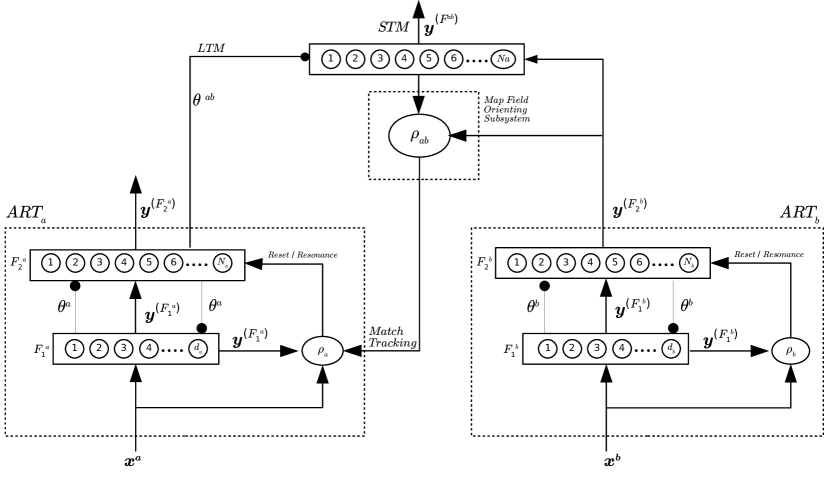
ART models used for supervised learning applications typically follow an ARTMAP architecture (Fig. 2), which consists of two elementary ART units (ART_a and ART_b) interconnected by an associative learning network, namely the map field, that performs multidimensional mappings between categories of both such units, as well as allowing for associative recalls when the input to one of the ART modules is missing. Notably, ARTMAP models usually inherit the properties of their elementary ART building blocks. This section describes the main characteristics of members of the supervised ART family in terms of their map field LTM units, dynamics (which encompasses activation, match, resonance criterion and learning) and user-defined parameters. For clarity, Table 5 summarizes the notation used in the following subsections.

Figure 2: Elementary ARTMAP model.

Table 5: Supervised ART models notation.

Notation Description $\bm{x}^{l}$ input sample to ART_$l$ $d_{l}$ input data dimensionality ($\bm{x}^{l}\in\mathbb{R}^{d_{l}}$) $F_{1}^{l}$ feature representation field of ART_$l$ $F_{2}^{l}$ category representation field of ART_$l$ F^ab map field $\bm{y}^{(F_{1}^{l})}$ $F_{1}^{l}$ activity (STM) $\bm{y}^{(F_{2}^{l})}$ $F_{2}^{l}$ activity (STM) $N_{l}$ number of categories in ART_$l$ $c^{l}$ a category in ART_$l$ $\bm{y}^{(F^{ab})}$ F^ab activity (STM) $\bm{\theta}^{ab}$ map field parameters (LTM unit) $M^{ab}$ map field match function $J$ ART_a chosen category index (via WTA) $K$ ART_b chosen category index (via WTA) $\rho_{l}$ vigilance parameter of ART_$l$ $\bar{\rho}$ ART_a baseline vigilance parameter

• Variable $l$ indexes the elementary ART module: $l=a,b$.

When an ARTMAP architecture is used for pattern recognition or classification tasks, typically ART_a clusters data samples while ART_b clusters class labels in parallel. Therefore, while ART maps samples to categories, an ARTMAP architecture goes one step further and maps categories to classes. During training, ART_a is subjected to a certain level of agreement with ART_b’s activity, given that the latter is encodes the target labels. This is performed by a second vigilance test that uses ART_b’s supervisory signal (i.e., response) to trigger a mismatch or allow learning given an incorrect or correct prediction, respectively. Specifically, when ART_a’s prediction is disproven by ART_b’s, then the map field triggers a match tracking mechanism in which ART_a’s resonating category is inhibited, the baseline vigilance is temporarily changed and the search process restarts, causing ART_a to select another category. Therefore, the map field is a critic, i.e., its purpose is to assess the quality of the mapping between both ART modules and also the necessity of adding a new node based on a supervised signal. Specifically, by engaging the match tracking mechanism, ARTMAP trades generalization for specificity to decrease training error. Often, ART_b is omitted and an $N_{b}$-dimensional vector of labels is used in its place (since ART_b’s vigilance parameter would typically be set to $1$, which would correspond to the number of categories being equal to the number of classes). Moreover, ART_a’s baseline vigilance parameter, which controls the granularity of the input space, is usually set to small values since this correlates with improved generalization capabilities and a higher level of compression, i.e., network complexity. Algorithm 2 summarizes the dynamics of an elementary ARTMAP model.

Input : $\{\bm{x}^{a},\bm{x}^{b}\}$, {ART_a and  ART_b parameters}, $\{\bm{\beta}_{ab},\bm{\gamma}_{ab},\bm{\rho}_{ab},\bm{\lambda}_{ab}\}$ (map field parameters).

Output : $\bm{y}^{(F^{ab})}$ (map field activity).

 

/* Notation

$\mathcal{C}_{l}$: set of ART_$l$ nodes ($l=a,b$).

$\bm{\theta}^{ab}$: map field LTM unit.

$\bm{\beta}_{ab}$: map field learning function parameter(s).

$\bm{\gamma}_{ab}$: map field match function parameter(s).

$\bm{\rho}_{ab}$: map field vigilance parameter(s).

$\bm{\lambda}_{ab}$: map field initialization parameter(s).

$f_{M}^{ab}(\cdot)$: map field match function.

$f_{L}^{ab}(\cdot)$: map field learning function.

$f_{V}^{ab}(\cdot)$: map field vigilance function.

$f_{N}^{ab}(\cdot)$: map field initialization function.

$f_{I}^{ab}(\cdot)$: map field inference function. */

/* Training */

1 Present input $\bm{x}^{b}\in\bm{X}^{b}$ to ART_b.

2 Perform the dynamics of ART_b and find its resonating category $K$ (Alg. 1).

3 Present input $\bm{x}^{a}\in\bm{X}^{a}$ to ART_a.

4 Perform the dynamics of ART_a and find its resonating category $J$ (Alg. 1).

5 Compute the map field match function: $M_{J}^{ab}=f_{M}^{ab}(J,K,\bm{\theta}^{ab},\bm{\gamma}_{ab})$.

6 Perform the map field vigilance test: $V_{J}=f_{V}^{ab}=\mathds{1}_{VR_{J}^{ab}}(\bm{x}^{a})$.

7 if $V_{J}$ is TRUE then

      8 Update ART_a’s and ART_b’s categories $J$ and $K$ (Alg. 1).

      

      9if ART_a OR ART_b created a new node then

            10 $\theta^{ab}_{|\mathcal{C}_{a}|+1}=f_{N}^{ab}(J,K,\bm{\lambda}_{ab})$.

            

      11 else

            12 Update the map field: $\theta^{ab}_{J}(new)=f_{L}^{ab}(\bm{x},\bm{\theta}_{J}^{ab}(old),\bm{\beta}_{ab})$.

            

      

13 else

      14 Inhibit ART_a’s category $J$ for $\bm{x}^{a}$.

      15 Go to step 2.

      

16Go to step 2.

/* Inference */

17 Present input $\bm{x}^{a}\in\bm{X}^{a}$ to ART_a.

18 Perform the dynamics of ART_a (Alg. 1).

19 Compute the degree of association to each ART_b node $k$ according to ART_a’s activity(s): $\sigma_{k}=f_{I}^{ab}(\bm{y}^{F_{2}^{a}},\bm{\theta}^{ab})$.

20 Set output: $y_{j}^{(F^{ab})}=\begin{cases}1,&\mbox{if }j=\operatorname*{arg\,max}\limits_{k}(\sigma_{k})\\ 0,&\mbox{otherwise}\end{cases}$.

Algorithm 2 Elementary ARTMAP algorithm.

3.1.1 ARTMAP

The first adaptive resonance theory supervised predictive mapping (predictive ART or ARTMAP) model [Carpenter et al., 1991a] consists of two binary ART 1 modules (Section 2.1.1), ART_a and ART_b, connected via an inter-ART associative memory, namely the map field F^ab. The latter performs multidimensional mappings between the binary input samples clustered by modules A and B. Moreover, when the input of a module is missing, it can be recalled by such associative memory. The map field LTM is represented by a matrix $\bm{W}^{ab}=[w^{ab}_{ij}]_{N_{a}\times N_{b}}$ such that $w^{ab}_{ij}=1$ if there is an association between category $i$ of ART_a and category $j$ of ART_b and zero otherwise, and $N_{a}$ and $N_{b}$ are the number of nodes in ART_a and ART_b, respectively. The matrix $\bm{W}^{ab}$ is initialized as $\bm{1}$ (i.e., the row vector $\bm{w}^{ab}_{1}=\vec{\bm{1}}$). The bottom-up and top-down weight vectors of both ART 1’s are initialized as described in Section 2.1.1.

Training. The map field F^ab activity is defined as

$$\bm{y}^{{(F^{ab})}}=\begin{cases}\bm{y}^{{(F_{2}^{b})}}\cap\bm{w}_{J}^{ab},&\mbox{if both ARTs are active (training)}\\ \bm{w}_{J}^{ab},&\mbox{if only ART\textsubscript{a} is active (prediction)}\\ \bm{y}^{{(F_{2}^{b})}},&\mbox{if only ART\textsubscript{b} is active}\\ \vec{\bm{0}},&\mbox{otherwise}\\ \end{cases}.$$ (96)

where $\bm{w}_{J}^{ab}=(w_{J1},...,w_{JN_{b}})$ is the $J^{th}$ row of $\bm{W}^{ab}$, which is associated with ART_a’s resonant category $J$.

After resonant nodes for both ART modules have been selected following the presentation of a sample pair $(\bm{x}^{a},\bm{x}^{b})$, the map field match function is computed as

$$M_{J}^{ab}=\frac{\|\bm{y}^{{(F^{ab})}}\|_{1}}{\|\bm{y}^{{(F_{2}^{b})}}\|_{1}}=\frac{\|\bm{y}^{{(F_{2}^{b})}}\cap\bm{w}_{J}^{ab}\|_{1}}{\|\bm{y}^{{(F_{2}^{b})}}\|_{1}},$$ (97)

where the vigilance test is satisfied if $M_{J}^{ab}\geq\rho_{ab}$. During training, if ART_a’s prediction is correct (i.e., confirmed by ART_b’s supervised signal feedback), all three modules learn. Otherwise, a match tracking mechanism (MT+) is engaged, such that ART_a’s vigilance parameter is temporarily raised by an amount small enough to inhibit the resonant category

$$\rho_{a}=M_{J}^{a}+\epsilon,~{}0<\epsilon\ll 1,$$ (98)

and the search process restarts. Either another resonant category is found or a new one is created, and the vigilance returns to its baseline value ($\rho_{a}=\bar{\rho}_{a}$) upon the presentation of a new input pair. Complement coding is usually employed to avoid cases in which ART_a’s vigilance is raised to a value greater than one.

Now consider that the resonant categories of ART_a and ART_b are $J$ and $K$, respectively. When the map field vigilance test is satisfied ($M_{J}^{ab}\geq\rho_{ab}$), then ART_a and ART_b are updated as described in Sec. 2.1.1, and the map field weight vector associated with category $J$ is updated as

$$w_{Jk}^{ab}(new)=\bm{y}^{(F_{2}^{b})}\cap\bm{w}_{J}^{ab}(old)=\begin{cases}1,&\mbox{if }k=K\\ 0,&\mbox{otherwise}\end{cases}$$ (99)

such that it becomes permanently associated with ART_b’s category $K$. Note that the $\text{F}_{\text{1}}^{\text{a}}$, $\text{F}_{\text{2}}^{\text{a}}$ and F^ab layers may be viewed as input, hidden and output layers, respectively.

Inference. In prediction mode, it is sufficient to track the map field’s weight vector $\bm{w}_{J}^{ab}$ and set it as the systems’ output, i.e., when an ART_a’s resonant category $J$ is found, the predicted class $K$ is obtained as

$$K=\operatorname*{arg\,max}\limits_{k}\left(\sigma_{k}\right),$$ (100)

where

$$\sigma_{k}=\sum\limits_{j=1}^{N_{a}}w^{ab}_{jk}y_{j}^{(F_{2}^{a})}.$$ (101)

A simplified ARTMAP version, namely the simple ARTMAP [Serrano-Gotarredona et al., 1998], replaces ART_b (and thus its $\text{F}_{\text{2}}^{\text{b}}$ activity $\bm{y}^{(F_{2}^{b})}$) with a binary vector $\bm{y}^{b}$ indicating the class membership of the input sample $\bm{x}^{a}$ (i.e., $y^{b}_{k}=1$ if $\bm{x}^{a}$ belongs to class $k$, and $y^{b}_{i}=0$ $\forall i\neq k$).

3.1.2 Fuzzy ARTMAP

Fuzzy ARTMAP (FAM) [Carpenter et al., 1992] is to ARTMAP what fuzzy ART is to ART 1: it extends the capabilities of ARTMAP to enable the processing of real-valued data by replacing logical with fuzzy AND intersection. Thus, fuzzy ARTMAP also consists of two fuzzy ART modules, ART_a and ART_b, connected by a map field F^ab that maps the categories of one ART to another via a matrix of weights $\bm{W}^{ab}$, as described in Sec. 3.1.1.

Training. The map field F^ab activity is defined as

$$\bm{y}^{{(F^{ab})}}=\begin{cases}\bm{y}^{{(F_{2}^{b})}}\wedge\bm{w}_{J}^{ab},&\mbox{if both ARTs are active (training)}\\ \bm{w}_{J}^{ab},&\mbox{if only ART\textsubscript{a} is active (prediction)}\\ \bm{y}^{{(F_{2}^{b})}},&\mbox{if only ART\textsubscript{b} is active}\\ \vec{\bm{0}},&\mbox{otherwise}\\ \end{cases}.$$ (102)

During training, ART_a and ART_b perform their dynamics (Section 2.1.3) simultaneously and independently, with their respective inputs, until both establish resonant nodes $J$ and $K$, respectively. Then, the map field computes its activity vector using these two pieces of information, as defined in Eq. (102). Next, a second (map field) vigilance test is performed to assess the mapping correctness using

$$M_{J}^{ab}=\frac{\lVert\bm{y}^{{(F^{ab})}}\rVert_{1}}{\lVert\bm{y}^{{(F_{2}^{b})}}\rVert_{1}}=\frac{\lVert\bm{y}^{{(F_{2}^{b})}}\wedge\bm{w}_{J}^{ab}\rVert_{1}}{\lVert\bm{y}^{{(F_{2}^{b})}}\rVert_{1}},$$ (103)

and, if it satisfies $M_{J}^{ab}\geq\rho_{ab}$ ($\rho_{ab}\in[0,1]$), then learning takes place. Otherwise, in response to a mismatch, the match tracking mechanism (M+) is triggered: the current resonating category $J$ is inhibited (lateral reset), ART_a’s vigilance parameter is raised by a small constant (Eq. (98)) and the search continues with the remaining nodes until a resonant category that satisfies both $\rho_{a}$ and $\rho_{ab}$ is either found or created. Finally, $\rho_{a}$ is reset to its baseline value $\rho_{a}=\bar{\rho}_{a}$ for the presentation of the following sample. However, the study in [Anagnostopoulos & Georgiopoulos, 2003] indicates that not using match tracking (MT+) reduces the computational burden and model complexity while improving generalization capabilities [Andonie & Sasu, 2006].

In both fuzzy ART modules learning is ensued as described in Section 2.1.3, whereas in the map field, its weight vectors are updated such that a permanent association is made between the active nodes of ART_a and ART_b

$$w_{Jk}^{ab}(new)=\bm{y}^{(F_{2}^{b})}\wedge\bm{w}_{J}^{ab}(old)=\begin{cases}1,&\mbox{if }k=K\\ 0,&\mbox{otherwise}\end{cases}.$$ (104)

Note that uncommitted nodes participate in the WTA competition. They are initialized as $\vec{\bm{1}}$, and the ART_a’s ones are mapped to all ART_b nodes. A slow-learning mode was introduced in [Carpenter et al., 1995]:

$$\bm{w}_{J}^{ab}(new)=\left(1-\beta_{ab}\right)\bm{w}_{J}^{ab}(old)+\beta_{ab}\left[\bm{y}^{{(F_{2}^{b})}}\wedge\bm{w}_{J}^{ab}(old)\right],$$ (105)

where $\beta_{ab}$ is the map field’s learning rate, and the conditional probability $p(c_{K}^{b}|c_{J}^{a})$ can be estimated nonparametrically as

$$\hat{p}(c_{K}^{b}|c_{J}^{a})=\dfrac{w_{JK}^{ab}}{\sum\limits_{i=1}^{N_{b}}w_{Ji}^{ab}}.$$ (106)

Inference. In testing mode only ART_a is active. Its output is used to make a prediction and concretely retrieve the labels from ART_b via the F^ab’s weight matrix (Eqs. (100) and (101)). Note that training, prediction/inference and learning are all WTA (based on a single category).

The simplified fuzzy ARTMAP (SFAM) [Kasuba, 1993] is a simplification of the original fuzzy ARTMAP specifically devised for classification tasks, in which, like simple ARTMAP in Sec. 3.1.1, ART_b is replaced by vectors indicating the class labels. Another simplified design is discussed in [Vakil-Baghmisheh & Pavešić, 2003].

3.1.3 Fuzzy Min-Max

Fuzzy Min-Max [Simpson, 1992] is a supervised learning neural network classifier that uses fuzzy sets for its internal categories, like its clustering counterpart (Sec. 2.1.4). It is composed of three layers of neurons: an input layer F_A, a layer of hyperbox nodes F_B and a layer of class nodes F_C. The hyperbox fuzzy sets are adjusted using an expansion-and-contraction-based fuzzy min-max classification learning algorithm that adjusts the fuzzy associations between the inputs and classes. It accomplishes that by identifying which hyperbox to expand for each input and expanding it correspondingly. Then, it identifies any resulting overlap between hyperboxes of different classes and minimally adjusts these hyperboxes to eliminate the overlap.

3.1.4 Fusion ARTMAP

Fusion ARTMAP [Asfour et al., 1993] is a modular neural network model designed to classify data originating from multiple sources (i.e., to perform sensor fusion). It generalizes fuzzy ARTMAP (Sec. 3.1.2) by incorporating multiple ART modules, one for each sensor. The outputs of these local ART modules are fed to a fuzzy ARTMAP, specifically, to the latter’s ART_a module, since ART_b receives the class labels. Another key feature of fusion ARTMAP is the parallel match tracking. Following an incorrect prediction, the vigilance parameter of each ART module is raised (individual ARTs and fuzzy ARTMAP’s ART_a)

$$\rho_{k}=\bar{\rho}_{k}+\Delta\rho,~{}\forall k,$$ (107)

$$\Delta\rho=\left(M_{J}^{n}-\bar{\rho}_{n}\right)+\epsilon,$$ (108)

$$n=\operatorname*{arg\,min}\limits_{k}\left(M_{J}^{k}\right),$$ (109)

where $\rho_{k}$ and $\bar{\rho}_{k}$ are the vigilance and baseline vigilance of ART module $k$, respectively. Each ART module can have its own baseline vigilance parameter, or the entire fusion ARTMAP system can have a single common baseline vigilance. The variable $M_{J}^{k}$ is the match function value of ART module $k$’s category $J$. Note that ART module $n$ yielded the smallest match value and is therefore deemed the least predictive.

The vigilance values of the local ART modules and fuzzy ARTMAP’s ART_a are increased by the same value, which is enough to promote a mismatch in ART module $n$. Therefore, the latter is forced to promote a new search, while the other modules maintain their output. This procedure enables credit assignment to specific modules instead of uniformly blaming all modules regardless of their predictive power. Fusion ARTMAP improves memory compression (compared to single-ART module systems that concatenate all sensor data into a single large vector) given the sharing of the local ART’s weight vectors across fuzzy ARTMAP.

The generalized symmetric fusion ARTMAP [Asfour et al., 1993] replaces fuzzy ARTMAP with a global ART module that receives the outputs of all local ART modules and is responsible for the decision-making process. This model can handle multiple input sensors and multiple supervised inputs. In cases consisting of only one supervised input, the functionality is reduced to fusion ARTMAP.

3.1.5 LAPART

The LAPART 1 [Healy et al., 1993] and LAPART 2 [Healy & Caudell, 1998] neural networks are two ART-based logic inference and supervised learning architectures. The LAPART 1 architecture uses two ART 1 networks $A$ and $B$ to learn logic inference and association, wherein if network $A$ assigns its input sample to a category, that results in network $B$ assigning its input to the corresponding category. It then uses the learned inference associations between the two networks to test hypotheses and classification decisions. The LAPART 2 algorithm uses the same architecture but introduces a lateral reset procedure and builds a rule extraction network that was shown to converge in two passes through the training data.

3.1.6 ART-EMAP

Adaptive resonance theory with spatial and temporal evidence integration (ART-EMAP) [Carpenter & Ross, 1995] augments fuzzy ARTMAP with a number of features to deal with noisy or ambiguous data: distributed representation during inference, integration of spatial-time information, extension of the map field into a multiple field EMAP module and a fine-tuning unsupervised learning stage (rehearsal).

Training. ART-EMAP training is identical to fuzzy ARTMAP’s (Sec. 3.1.2).

Inference. ART-EMAP introduces two contrast enhancement procedures for distributed activation: the normalized power rule defined as

$$y_{j}^{(F_{2}^{a})}=\frac{(T_{j}^{a})^{p}}{\sum\limits_{i=1}^{N_{a}}(T_{i}^{a})^{p}}~{},~{}p>1,$$ (110)

and the threshold rule

$$y_{j}^{(F_{2}^{a})}=\frac{[T_{j}^{a}-T]^{+}}{\sum\limits_{i=1}^{N_{a}}[T_{i}^{a}-T]^{+}}$$ (111)

where $T$ is a threshold parameter, and $[\xi]^{+}=\max\{0,\xi\}$ is a rectifier operation. The activity of the first map field $F_{1}^{ab}$ is then defined as

$$\bm{y}^{(F_{1}^{ab})}=\bm{S}^{ab}$$ (112)

where

$$S^{ab}_{k}=\sum\limits_{j=1}^{N_{a}}w_{jk}^{ab}y_{j}^{(F_{2}^{a})},$$ (113)

A class is predicted using such distributed representation via the second map field activity $F_{2}^{ab}$

$$y_{k}^{(F_{2}^{ab})}=\begin{cases}1,&\mbox{if }k=K\\ 0,&\mbox{otherwise}\end{cases},$$ (114)

where

$$K=\operatorname*{arg\,max}\limits_{k}\left[y_{k}^{(F_{1}^{ab})}\right].$$ (115)

To address ambiguity (i.e., categories with similar activation values), the $F_{2}^{ab}$ activity can be redefined as:

$$y_{k}^{(F_{2}^{ab})}=\begin{cases}1,&\mbox{if }y_{k}^{(F_{1}^{ab})}>(DC)y_{j}^{(F_{1}^{ab})}~{}~{}\forall j\neq k\\ 0,&\mbox{otherwise}\end{cases}$$ (116)

where $DC\geq 1$ is a decision criterion. While $\bm{y}_{k}^{(F_{2}^{ab})}=\vec{\bm{0}}$, the system waits for another input (i.e., data samples from the same and yet unknown class) until the inequality in Eq. (116) is satisfied. Moreover, the power rule can also be applied to the $F_{1}^{ab}$ activity

$$y_{k}^{(F_{1}^{ab})}=\frac{(S_{k}^{ab})^{q}}{\sum\limits_{i=1}^{N_{b}}(S_{i}^{ab})^{q}}~{},~{}q>1,$$ (117)

where the $q$ is the power parameter.

To handle noisy environments, ART-EMAP uses a map evidence accumulation field $F_{E}^{ab}$ that combines information from multiple $F_{1}^{ab}$ activities over time:

$$T_{k}^{ab}(new)=T_{k}^{ab}(old)+y_{k}^{(F_{1}^{ab})},$$ (118)

where $T_{k}^{ab}$ is the evidence accumulating MTM. It is initialized as zero ($\bm{T}^{ab}=\vec{\bm{0}}$) and reset once the DC is satisfied. The $F_{2}^{ab}$ activity can then be redefined as

$$y_{k}^{(F_{2}^{ab})}=\begin{cases}1,&\mbox{if }T_{k}>(DC)T_{j}~{}~{}\forall j\neq k\\ 0,&\mbox{otherwise}\end{cases},$$ (119)

where improved accuracy correlates with larger $DC$ values and a greater number of samples [Carpenter & Ross, 1995].

Finally, to learn from the samples used to disambiguate prediction, an unsupervised learning stage (“rehearsal”) takes place. In this fine-tuning stage, the LTMs of ART_a, ART_b and the map field maintain their values, whereas another set of weights from $\text{F}_{\text{2}}^{\text{a}}$ to $\text{F}_{\text{E}}^{\text{ab}}$ is adapted when such samples are re-presented to the system.

3.1.7 Adaptive resonance associative map

The fuzzy adaptive resonance associative map (ARAM) [Tan, 1995] extends ART autoassociative to heteroassociative mappings by connecting two ARTs (A and B) via a common category representation field F₂.

LTM. Fuzzy ARAM has two F₁ layers connected to a single F₂ layer whose LTM unit is $\bm{\theta}=\{\bm{w}=[\bm{w}^{a},\bm{w}^{b}]\}$.

Activation. When normalized and complement coded inputs ($\bm{x}=[\bm{x}^{a},\bm{x}^{b}]$) are presented, the activation function is computed as

$$T_{j}=\gamma\dfrac{|\bm{x}^{a}\wedge\bm{w}_{j}^{a}|}{\alpha_{a}+|\bm{w}_{j}^{a}|}+(1-\gamma)\dfrac{|\bm{x}^{b}\wedge\bm{w}_{j}^{b}|}{\alpha_{b}+|\bm{w}_{j}^{b}|},$$ (120)

where $\gamma\in[0,1]$ is the contribution parameter. Note that there is an independent set of parameters for each module: choice parameters $\alpha_{m}>0$, learning parameters $\beta_{m}\in[0,1]$ and vigilance parameters $\rho_{m}\in[0,1]$, where $m\in\{a,b\}$.

Match and resonance. Consider that node $J$ has been selected via a WTA competition. F₁ and F₂ activities are defined as:

$$y_{j}^{(F_{1}^{m})}=\begin{cases}\bm{x}^{m},&\mbox{if $F_{2}^{m}$ is inactive}\\ \bm{x}^{m}\wedge\bm{w}_{J}^{m},&\mbox{otherwise}\end{cases},$$ (121)

where $m\in\{a,b\}$, and

$$y_{j}^{(F_{2})}=\begin{cases}1,&\mbox{if }j=J\\ 0,&\mbox{otherwise}\end{cases}.$$ (122)

The match functions are computed for node $J$ as

$$M_{J}^{m}=\frac{\lVert\bm{y}^{(F_{1}^{m})}\rVert_{1}}{\lVert\bm{x}^{m}\rVert_{1}}=\frac{\lVert\bm{x}^{m}\wedge\bm{w}_{J}^{m}\rVert_{1}}{\lVert\bm{x}^{m}\rVert_{1}},$$ (123)

and resonance occurs if $M_{J}^{m}\geq\rho_{m}$ for both $m\in\{a,b\}$ simultaneously. Thus, $VR_{J}=\{[\bm{x}^{a},\bm{x}^{b}]:$ $M_{J}^{a}(\bm{x}^{a})\geq\rho_{a}$ and $M_{J}^{b}(\bm{x}^{b})\geq\rho_{b}\}$. In this case, learning is ensued such that the weights $\bm{w}_{J}^{m}$ are updated using fuzzy ART’s learning rule (Eq. (22) in Sec. 2.1.3). Otherwise, a match tracking mechanism temporarily raises the baseline $\bar{\rho}_{a}$ (which is reset at the start of each sample presentation) as in fuzzy ARTMAP (Sec. 3.1.2), and the search for another resonant category continues. If an uncommitted category is recruited, then another one is initialized as $\bm{w}^{m}=\vec{\bm{1}}$. Specifically, when such dynamics take place and $\gamma=1$, fuzzy ARAM is functionally equivalent to fuzzy ARTMAP [Tan, 1995].

3.1.8 Gaussian ARTMAP

The Gaussian ARTMAP (GAM) [Williamson, 1996] is a discriminative model [Vigdor & Lerner, 2007] that uses Gaussian ART elementary units (Sec. 2.1.6) as building blocks.

Training. Training follows the standard ARTMAP dynamics (Sec. 3.1.1), where the match tracking mechanism is triggered following a predictive error.

Inference. During testing mode, predictions are made considering the total probability of each classes, i.e., by using Eqs. (100) and (101) with $y_{j}^{(F_{2}^{a})}=T_{j}^{a}$ (Eq. (33)).

3.1.9 Probabilistic fuzzy ARTMAP

The probabilistic fuzzy ARTMAP (PFAM) [Lim & Harrison, 1997a, 2000a] combines fuzzy ARTMAP’s code compression ability (Sec. 3.1.2) with the probability density function estimation of probabilistic neural networks (PNN) [Specht, 1990] in a hybrid system: during training, a fuzzy ARTMAP variant is used to generate prototypes in a supervised manner, whereas during inference, the PNN uses Bayes decision theory to make predictions.

Training. Training is similar to fuzzy ARTMAP, except for the following:

1. Map field dynamics: the activity of F^ab used to compute the match function (Eq. (103) in Sec. 3.1.2) is defined as

   $$\bm{y}^{{(F^{ab})}}=\bm{y}^{{(F_{2}^{b})}}\wedge\frac{\bm{w}_{J}^{ab}}{\lVert\bm{w}_{J}^{ab}\rVert_{1}},$$ (124)

   and when learning is ensued, $\bm{W}^{ab}$ is updated using

   $$\bm{w}_{J}^{ab}(new)=\bm{w}_{J}^{ab}(old)+\bm{y}^{{(F^{ab})}};$$ (125)

2. If the match tracking mechanism is engaged, then the condition

   $$0\leq\rho_{a}\leq\min\left(1,M_{J}^{a}+\epsilon\right),~{}0<\epsilon\ll 1,$$ (126)

   is enforced to enable identical categories to be associated with different classes [Lim & Harrison, 1997b];

3. Centroids $\bm{\mu}_{j}^{a}$ are embedded in ART_a (i.e., the LTM unit is $\bm{\theta}=\{\bm{w},\bm{\mu}\}$). These are initialized as $\bm{\mu}_{j}^{a}=\vec{\bm{0}}$ and recursively estimated using

   $$\bm{\mu}_{j}^{a}(new)=\bm{\mu}_{j}^{a}(old)+\frac{1}{\lVert\bm{w}_{J}^{ab}\rVert_{1}}\left(\bm{x}^{a}-\bm{\mu}_{j}^{a}(old)\right),$$ (127)

   where $\bm{x}^{a}$ is complement coded for fuzzy ARTMAP categories $\bm{w}$ but not for the centroids $\bm{\mu}$.

Inference. Prediction is accomplished using the maximum a posteriori (MAP) or minimum-risk estimate:

$$\hat{p}(c_{k}^{b}|\bm{x}^{a})=\hat{p}(\bm{x}^{a}|c_{k}^{b})\hat{p}(c_{k}^{b})l(c_{jk}),$$ (128)

where $l(c_{jk})$ represents the cost of selecting $c_{k}^{b}$ when in fact the true class is $c_{j}^{b}$. The prior probability estimate of a given class $k$ is given by the ratio of the number of samples encoded by ART_a’s prototypes that are mapped to class $k$ to the total number of samples presented to PFAM:

$$\hat{p}(c_{k}^{b})=\dfrac{\sum\limits_{j=1}^{N_{a}}w_{jk}^{ab}}{\sum\limits_{k=1}^{N_{b}}\sum\limits_{j=1}^{N_{a}}w_{jk}^{ab}},$$ (129)

and $p(\bm{x}^{a}|c_{k}^{b})$ is estimated using the Parzen-window method [Parzen, 1962, Cacoullos, 1966] with isotopic Gaussians kernels ($\bm{\Sigma}_{j}=\sigma_{j}^{2}\bm{I}$)

$$\hat{p}(\bm{x}^{a}|c_{k}^{b})=\sum\limits_{j=1}^{N_{a}}\dfrac{\mathds{1}_{c_{k}^{b}}(\bm{\mu}_{j}^{a})}{\sum\limits_{i=1}^{N_{a}}\mathds{1}_{c_{k}^{b}}(\bm{\mu}_{i}^{a})}\frac{e^{\left(-\frac{\lVert\bm{x}^{a}-\bm{\mu}_{j}^{a}\rVert_{2}^{2}}{2\sigma_{j}^{2}}\right)}}{\left(2\pi\right)^{\frac{d}{2}}\sigma_{j}^{d}},$$ (130)

where

$$\mathds{1}_{c_{k}^{b}}(\bm{\mu}_{j}^{a})=\begin{cases}1,&\mbox{if }\bm{\mu}_{j}^{a}\in c_{k}^{b}\\ 0,&\mbox{otherwise}\end{cases}.$$ (131)

The kernels used for the realization of the Parzen-window density estimation have heteroscedastic components, which are computed as

$$\sigma_{j}=\frac{1}{r}\min\limits_{i}\lVert\bm{\mu}_{j}^{a}-\bm{\mu}_{i}^{a}\rVert_{2},$$ (132)

or determined using the $k$-nearest neighbors method [Duda et al., 2000]

$$\sigma_{j}=\frac{1}{k}\sum\limits_{i=1}^{k}\|\bm{\mu}_{j}^{a}-\bm{\mu}_{i}^{a}\|,~{}1\leq k\leq N_{a}-1,$$ (133)

where $r$ is a user-defined overlapping parameter, and $\bm{\mu}_{j}^{a}$ and $\bm{\mu}_{i}^{a}$ belong to different classes in Eqs. (132) and (133).

3.1.10 ARTMAP-IC

The ARTMAP-IC model [Carpenter & Markuzon, 1998] is a fuzzy ARTMAP variant whose key characteristics are (i) a new match tracking mechanism (MT-) to reduce model complexity and (ii) the inclusion of instance counting (via a new counting field F₃) for probabilistic distributed prediction.

ARTMAP-IC replaces ART_b with a vector $\bm{y}^{b}$ encoding the classes of the classification problem, such that, for a given input $\bm{x}^{a}$ presented to ART_a,

$$y_{i}^{b}=\begin{cases}1,&\mbox{if }\bm{x}^{a}\in\mbox{ class }i\\ 0,&\mbox{otherwise}\end{cases},$$ (134)

The activity of the counting field F₃ (located in-between ART_a and F^ab) is defined as

$$y_{j}^{(F_{3})}=\begin{cases}y_{j}^{(F_{2}^{a})},&\mbox{training}\\ \dfrac{c_{j}y_{j}^{(F_{2}^{a})}}{\sum\limits_{i=1}^{N_{a}}c_{i}y_{i}^{(F_{2}^{a})}},&\mbox{prediction}\end{cases},$$ (135)

where the instance counting weight $c_{j}$ records the number of samples that are encoded by category $j$, i.e., the number of times it is activated. The map field F^ab activity can then be defined as

$$\bm{y}^{{(F^{ab})}}=\begin{cases}\bm{y}^{b}\wedge\bm{U},&\mbox{ training}\\ \bm{U},&\mbox{ prediction}\\ \end{cases}$$ (136)

where the kth component of the map field’s input is

$$U_{k}=\sum\limits_{j=1}^{Na}w_{jk}^{ab}y_{j}^{(F_{3})},k=1,...,N_{b},$$ (137)

and here $N_{b}$ represents the number of classes.

Training. During training, the match function is defined as

$$M_{J}^{ab}=\frac{\lVert\bm{y}^{b}\wedge\bm{U}\rVert_{1}}{\lVert\bm{y}^{b}\rVert_{1}}=\lVert\bm{y}^{b}\wedge\bm{w}_{J}^{ab}\rVert_{1},$$ (138)

since $\bm{U}=\bm{w}_{J}^{ab}$ (because $\bm{y}^{(F_{2}^{a})}=\bm{y}^{(F_{3})}$) and $\lVert\bm{y}^{b}\rVert_{1}=1$. If the vigilance criterion is not satisfied ($M_{J}^{ab}<\rho_{ab}$), then the new match tracking mechanism (MT-) is engaged such that ART_a’s vigilance is set to

$$\rho_{a}(new)=M_{J}^{a}+\epsilon,~{}\epsilon\leq 0\mbox{ and }\|\epsilon\|\mbox{ small},$$ (139)

and the search proceeds as with fuzzy ARTMAP. Otherwise, if learning is ensued, then fuzzy ART_a and the map field weight vectors learn as described in Secs. 2.1.3 and 3.1.2, respectively. The instance counting is updated as

$$c_{j}(new)=c_{j}(old)+y_{j}^{(F_{2}^{a})},$$ (140)

where $c_{j}$’s are initialized as 0.

Inference. During testing, no search occurs, and ARTMAP-IC uses the Q-max rule to distribute $\text{F}_{\text{2}}^{\text{a}}$ activity via the following contrast enhancement procedure:

$$y_{j}^{(F_{2}^{a})}=\begin{cases}\dfrac{T_{j}}{\sum\limits_{\lambda\in\Lambda}T_{\lambda}},&\mbox{if }j\in\Lambda\\ 0,&\mbox{otherwise}\end{cases},$$ (141)

where $\Lambda$ is the set formed by the $Q$ categories with the largest activation values ($Q$ is a user-defined parameter). This is similar to k-nearest neighbors [Duda et al., 2000] where $Q$ assumes the role of $k$ [Carpenter & Markuzon, 1998]. Setting $Q=1$ leads to WTA mode.

Finally, the probability of class $k$ is then computed as

$$\sigma_{k}=\dfrac{U_{k}}{\sum\limits_{l=1}^{N_{b}}U_{l}}=\dfrac{\sum\limits_{j\in\Lambda}w_{jk}^{ab}c_{j}T_{j}}{\sum\limits_{l=1}^{N_{b}}\sum\limits_{j\in\Lambda}w_{jl}^{ab}c_{j}T_{j}}.$$ (142)

3.1.11 Distributed ARTMAP

Distributed ARTMAP (dARTMAP) [Carpenter et al., 1998] was developed to improve supervised ART models regarding model compactness and noise robustness (i.e., reduce category proliferation) while performing fast and stable learning via distributed representation. It features distributed activation, match and learning functions. Notably, distributed ARTMAP generalizes the following supervised ART models [Carpenter, 2003]: “dARTMAP $\supset$ ARTMAP-IC $\supset$ default ARTMAP $\supset$ fuzzy ARTMAP”, where $\supset$ is used to indicate containment considering this ARTMAP’s ecosystem.

In case of classification problems, distributed ARTMAP uses distributed ART (Sec. 2.1.5) as a building block for ART_a, while replacing ART_b with a binary vector indicating the input’s class membership (Eq. (134) in Sec. 3.1.10). The distributed ARTMAP uses an increased-gradient content-addressable memory (IG CAM) rule for contrast enhancement. A CAM rule defines a function that yields the steady state values of the network’s STM when an input sample is presented. Particularly, distributed ARTMAP’s CAM rule defines a power function that is controlled by a parameter $p$. The latter has a role akin to the variance in Gaussian kernels, and, as it tends to infinity, the network converges to WTA.

Training. During training, the distributed ARTMAP alternates between distributed and WTA modes. Like ARTMAP-IC (Sec. 3.1.10), distributed ARTMAP features a counting field $\text{F}_{\text{3}}^{\text{a}}$ (for instance counting purposes) which is cascaded to $\text{F}_{\text{2}}^{\text{a}}$ and employs the MT- match tracking search algorithm. Briefly, the distributed representation undergoes the unsupervised (Eqs. (26) to (28)) and supervised vigilance (i.e., prediction assessment) tests, and if one of them fails the system switches to WTA mode and its corresponding dynamics are carried out (in which nodes can be added incrementally). Otherwise, distributed mode dynamics take place.

Particularly, the distributed ARTMAP uses the distributed choice-by-difference activation function (Eq. (23) in Sec. 2.1.5 disregarding the depletion parameters)

$$T_{j}=\sum\limits_{i=1}^{2d}\left[x_{i}^{a}\wedge(1-\tau_{i}^{bu})\right]+(1-\alpha)\sum\limits_{i=1}^{2d}\tau_{i}^{bu},~{}\alpha\in(0,1),$$ (143)

and, after these are computed, the following subsets of highly active nodes are considered:

1. $\Lambda=\{j:T_{j}\geq T^{u}\}$

2. $\Lambda^{\prime}=\{j:T_{j}=(2-\alpha)d\}$

where $T^{u}$ is the activation function of an uncommitted node ($\bm{\tau}^{bu}=\bm{\tau}^{td}=\vec{\bm{0}}$). The IG CAM rule specifies the following functions for the steady-state activities of distributed ARTMAP’s modes

• Distributed mode

  • If $\Lambda^{\prime}\neq\{\emptyset\}$, then

    $$y_{j}^{(F_{2}^{a})}=\begin{cases}\dfrac{1}{|\Lambda^{\prime}|},&\forall j\in\Lambda^{\prime}\\ 0,&\mbox{otherwise}\end{cases},$$ (144)

    where $|\cdot|$ represents the cardinality of a set.

  • If $\Lambda^{\prime}=\{\emptyset\}$ and $\Lambda\neq\{\emptyset\}$, then

    $$y_{j}^{(F_{2}^{a})}=\begin{cases}\dfrac{1}{1+\sum\limits_{\lambda\in\Lambda,\lambda\neq j}\left[\dfrac{(2-\alpha)d-T_{j}}{(2-\alpha)d-T_{\lambda}}\right]^{p}},&\forall j\in\Lambda\\ 0,&\mbox{otherwise}\end{cases}$$ (145)

  where $p\in(0,\infty)$ is the power parameter. The ART_a’s counting field F₃ activity is then defined as

  $$y_{j}^{(F_{3}^{a})}=\dfrac{c_{j}y_{j}^{(F_{2}^{a})}}{\sum\limits_{\lambda=1}^{C}c_{\lambda}y_{\lambda}^{(F_{2}^{a})}},$$ (146)

  where $C$ is the number of ART_a’s committed nodes, and $c_{j}$ is the instance counting of node $j$ (if uncommitted, then $c_{j}=0$). The signal used in the ART_a’s match function is then

  $$\sigma_{i}=\sum\limits_{j=1}^{C}\left[y_{j}^{(F_{3}^{a})}-\tau^{td}_{j,i}\right]^{+},~{}i=1,...,2d.$$ (147)

• WTA mode

  • If $\Lambda\neq\{\emptyset\}$, then the winner node is $J=\operatorname*{arg\,max}\limits_{j\in\Lambda}{(T_{j})}$.

  • If $\Lambda=\{\emptyset\}$, then the uncommitted node is recruited to learn the presented input sample.

  The ART_a’s counting field F₃ activity is then

  $$y_{j}^{(F_{3}^{a})}=y_{j}^{(F_{2}^{a})}=\begin{cases}1,&\mbox{if }j=J\\ 0,&\mbox{otherwise}\end{cases},$$ (148)

  and the signal used in the ART_a’s match function is

  $$\sigma_{i}=\left(1-\tau^{td}_{J,i}\right),~{}i=1,...,2d.$$ (149)

If the vigilance test of ART_a is not satisfied (Eqs. (26) to (28)) in Sec. 2.1.5), then distributed ARTMAP reverts to WTA mode, and the search continues until a resonant node is either found or created. Finally, the output class is then estimated using Eqs. (100) and (101) with $y_{j}^{(F_{3}^{a})}$ in place of $y_{j}^{(F_{2})}$. If the prediction is incorrect, then match tracking is engaged using the MT- algorithm (Sec. 3.1.10). Otherwise, ART_a adapts using the distributed ART learning laws described in Sec. 2.1.5 (the top-down thresholds components are updated using $y_{j}^{(F_{3}^{a})}$ in place of $y_{j}^{(F_{2})}$ in Eq. (31)), and the instance countings are updated using Eq. (140) in Sec. 3.1.10.

Note that if the distributed ARTMAP system enters a resonant state while in distributed mode, then, prior to learning, a credit assignment stage takes place in which the nodes permanently associated with the wrong class are inhibited, the $\text{F}_{\text{2}}^{\text{a}}$ activity is re-normalized (i.e., $\lVert\bm{y}^{(F_{2}^{a})}\rVert_{1}=1$) and the $\text{F}_{\text{3}}^{\text{a}}$ activity and the signal $\bm{\sigma}$ are recomputed using Eqs. (146) and (147), respectively.

Inference. To make a prediction for a new sample $\bm{x}$, distributed ARTMAP operates similarly to the training phase but always in distributed mode and with search and learning disabled (i.e., in feedforward mode).

3.1.12 Hypersphere ARTMAP

Hypersphere ARTMAP (HAM) [Anagnostopoulos & Georgiopulos, 2000] closely follows the operation of fuzzy ARTMAP (Sec. 3.1.2) but instead uses hypersphere ART (Sec. 2.1.7) modules for ART_a and ART_b. ART_b is responsible for clustering the classes ($\bm{x}^{b}$), ART_a does the data samples ($\bm{x}^{a}$) and the inter-ART maps the ART_a categories to the ART_b categories regulated by the match tracking procedure.

3.1.13 Ellipsoid ARTMAP

Similar to hypersphere ARTMAP, ellipsoid ARTMAP (EAM) [Anagnostopoulos & Georgiopoulos, 2001a, b] uses ellipsoid ART (Sec. 2.1.8) for both its ART_a and ART_b modules while closely following the fuzzy ARTMAP’s operation (Sec. 3.1.2).

3.1.14 µARTMAP

The $\mu$ARTMAP model [Sanchez et al., 2000, Gomez-Sanchez et al., 2002] is a fuzzy ARTMAP variant developed to reduce the type of category proliferation due to overlapping classes, consequently improving generalization capability. This is accomplished by regulating the conditional entropy between the input (ART_a) and output (ART_b) spaces

$$H(ART_{b}|ART_{a})=\sum\limits_{j=1}^{N_{a}}h_{j},$$ (150)

where $h_{j}$ is the contribution of ART_a’s node $j$ to the total entropy:

$$h_{j}=-\hat{p}(c_{j}^{a})\sum\limits_{k=1}^{N_{b}}\hat{p}(c_{k}^{b}|c_{j}^{a})\log_{2}\hat{p}(c_{k}^{b}|c_{j}^{a}),$$ (151)

and the probabilities are estimated using the map field’s LTM unit, whose dynamics are similar to PROBART’s (Sec. 3.2.1). This process indirectly controls the training error, which is relaxed to address overfitting.

Training. Training is divided into two phases, and the first one is performed online. Assuming the resonant categories of ART_a and ART_b are $J$ and $K$, respectively, the map field vigilance test is defined using Eq. (151):

$$M_{J}^{ab}=h_{J},$$ (152)

where

$$p(c_{k}^{b}|c_{j}^{a})=\begin{cases}\dfrac{y^{(F^{ab})}_{k}}{\lVert\bm{y}^{(F^{ab})}\rVert_{1}},&\mbox{if }j=J\\ \dfrac{w^{ab}_{jk}}{\lVert\bm{w}^{ab}_{j}\rVert_{1}},&\mbox{ otherwise}\end{cases},$$ (153)

$$p(c_{j}^{a})=\begin{cases}\dfrac{\lVert\bm{y}^{(F^{ab})}\rVert_{1}}{\lVert\bm{y}^{(F^{ab})}\rVert_{1}+\sum\limits_{i=1,i\neq J}^{N_{a}}\lVert\bm{w}^{ab}_{i}\rVert_{1}},&\mbox{if }j=J\\ \dfrac{\lVert\bm{w}^{ab}_{j}\rVert_{1}}{\lVert\bm{y}^{(F^{ab})}\rVert_{1}+\sum\limits_{i=1,i\neq J}^{N_{a}}\lVert\bm{w}^{ab}_{i}\rVert_{1}},&\mbox{ otherwise}\end{cases}.$$ (154)

Note, however, that if $J$ is an uncommitted node, then

$$p(c_{k}^{b}|c_{J}^{a})=\begin{cases}1,&\mbox{if }k=K\\ 0,&\mbox{ otherwise}\end{cases},$$ (155)

which implies $h_{J}=0$. The value of $h_{J}$ measures the homogeneity of ART_b nodes (i.e., classes) associated with ART_a’s category $J$. If $M_{J}^{ab}\leq h_{max}$, where $h_{max}$ is a user-defined parameter, then the map field vigilance is satisfied and learning is ensued as in PROBART (Eq. (209)). Otherwise, ART_a’s node $J$ is inhibited, and the search continues without changing ART_a’s vigilance parameter. Note that $h_{max}=0$ implies mapping to a single class, whereas $h_{max}>0$ allows mapping to different classes (i.e., non-zero training error).

Next, an offline training phase is performed to measure the overlap between categories. In this second training phase no learning is permitted within the ART modules. Probabilities are re-estimated using

$$p(c_{k}^{b}|c_{j}^{a})=\dfrac{v^{ab}_{jk}}{\lVert\bm{v}^{ab}_{j}\rVert_{1}},$$ (156)

$$p(c_{j}^{a})=\dfrac{\lVert\bm{v}^{ab}_{j}\rVert_{1}}{\sum\limits_{i=1}^{N^{a}}\lVert\bm{v}^{ab}_{i}\rVert_{1}},$$ (157)

where a temporary map field co-occurrence matrix $\bm{V}^{ab}$ is updated in a unsupervised manner, i.e., without match tracking (Initialization: $\bm{V}^{ab}=\bm{0}$). The total entropy $H$ is computed using Eq. (150), and if $H>H_{max}$, where $H_{max}$ is a user-defined parameter, then the mapping is considered too entropic. ART_a’s category $M$ with the largest contribution $h_{M}$ is removed, and the baseline vigilance $\bar{\rho}_{a}$ is increased for all new uncommitted categories as

$$\bar{\rho}_{a}=\dfrac{\lVert\bm{w}_{M}^{a}\rVert_{1}}{\lVert\bm{x}^{a}\rVert_{1}}+\epsilon,$$ (158)

thus adaptively tuning individual vigilance parameters of ART_a’s categories. The samples that were associated with node $M$ are re-presented and the learning process resumes. This entire process is repeated until $H\leq H_{max}$, in which the training stops. Notably, if $h_{max},H_{max}\geq\log_{2}N_{b}$ then $\mu$ARTMAP behaves similarly to PROBART, whereas if $h_{max}=0$ and $H_{max}\geq\log_{2}N_{b}$, then $\mu$ARTMAP behaves similarly to fuzzy ARTMAP.

Inference. Predictions are made using Eqs. (100) and (101), i.e., the class output $K$ is estimated as the one that has the largest frequency of association with ART_a’s resonant category $J$.

Under certain conditions, $\mu$ARTMAP creates large categories that lead to considerable overlaps and decrease the system’s performance. The safe-$\mu$ARTMAP [Gomez-Sanchez et al., 2001] variant is a generalization of $\mu$ARTMAP that adds another vigilance criterion to mediate learning. Specifically, to avoid the formation of large hyperrectangles that enclose far apart samples belonging to the same class, besides passing both the ART_a and the map field vigilance tests, an ART_a category also needs to undergo a distance criterion defined as

$$M_{J}^{\Delta w}=\dfrac{\lVert\bm{w}_{J}^{a}\rVert_{1}-\lVert\bm{w}_{J}^{a}\wedge\bm{x}^{a}\rVert_{1}}{\lVert\bm{x}^{a}\rVert_{1}}.$$ (159)

Only if this third vigilance test is also satisfied ($M_{J}^{\Delta w}\leq\delta$, $0<\delta<1-\rho$), then learning takes place. This imposes a restriction on the instantaneous change of a category size, which is upper bounded by $\lVert\bm{x}^{a}\rVert_{1}\delta$. Particularly, safe-$\mu$ARTMAP reduces to $\mu$ARTMAP when $\delta=1$ (which effectively implies the absence of a constraint).

3.1.15 Default ARTMAPs

The default ARTMAP 1 model [Carpenter, 2003] is characterized by the usage of a distributed representation to perform continuously-valued predictions, as opposed to binary and fuzzy ARTMAP models (Secs. 3.1.1 and 3.1.2), which use WTA code representation.

Training. Default ARTMAP 1’s training is akin to fuzzy ARTMAP’s, except for (i) the absence of ART_b (default ARTMAP 1 is a simplified architecture), (ii) its ART_a module employs the choice-by-difference activation function defined as [Carpenter & Gjaja, 1994]

$$T_{j}=\lVert\bm{x}\wedge\bm{w}_{j}^{a}\rVert_{1}+(1-\alpha)(d-\lVert\bm{w}_{j}^{a}\rVert_{1}),\alpha\in(0,1),$$ (160)

and (iii) the match tracking algorithm, which is MT- search [Carpenter & Markuzon, 1998].

Inference. As opposed to fuzzy ARTMAP, default ARTMAP 1 uses a distributed representation for inference, where two subsets of highly active neurons are selected as:

1. $\Lambda=\{\lambda=1,...,N_{a}:T_{\lambda}>\alpha d\}$

2. $\Lambda^{\prime}=\{\lambda=1,...,N_{a}:T_{\lambda}=d~{}(i.e.,~{}\bm{w}_{\lambda}=\bm{x}^{a})\}$

Next, the IG CAM rule is applied:

• If $\Lambda^{\prime}\neq\{\emptyset\}$, then

  $$y_{j}=\begin{cases}\dfrac{1}{|\Lambda^{\prime}|},&\forall j\in\Lambda^{\prime}\\ 0,&\mbox{otherwise}\end{cases},$$ (161)

  where $|\cdot|$ represents the cardinality of a set.

• If $\Lambda^{\prime}=\{\emptyset\}$, then

  $$y_{j}=\begin{cases}\frac{\left[\dfrac{1}{d-T_{j}}\right]^{p}}{\sum\limits_{\lambda\in\Lambda}\left[\dfrac{1}{d-T_{\lambda}}\right]^{p}},&\forall j\in\Lambda\\ 0,&\mbox{otherwise}\end{cases}.$$ (162)

Finally, the predictions for each class are obtained using Eqs. (100) and (101) in Sec. 3.1.1.

In a WTA system, such as fuzzy ARTMAP, after learning a sample, an immediate re-presentation is guaranteed to yield a correct prediction, i.e., it passes the “next-input-test”. However, the default ARTMAP 1 WTA prediction during training might not be the same as the distributed one. To overcome this problem, the default ARTMAP 2 model [Amis & Carpenter, 2007] introduces the “distributed-next-input-test” during training, to assure that a correct prediction would also be performed under a distributed representation. Briefly, in order to anticipate an error, after learning from a sample in a WTA mode, the prediction is verified again using a distributed representation. If the distributed prediction is correct, then learning resumes by returning to WTA mode and presenting the next sample. Otherwise, the match tracking mechanism is engaged, the system reverts to WTA mode, the resonant category is inhibited and the network restarts the search to learn more from that sample.

3.1.16 Boosted ARTMAP

Boosted ARTMAP [Verzi et al., 1998] is a variant of fuzzy ARTMAP (Sec. 3.1.2) closely related to PROBART [Marriott & Harrison, 1995] (Sec. 3.2.1). It is inspired by Boosting theory [Schapire, 1990] and was developed to improve the fuzzy ARTMAP’s generalization capability (since it is prone to overfitting the training data) and to create less complex networks (i.e., to reduce the type of category proliferation caused by overlapping classes). These are addressed by regulating the training error, which is allowed to be non-zero. Particularly, boosted ARTMAP’s ART_a and ART_b modules are boosted ART models (which are identical to fuzzy ART, except that the categories are endowed with individual vigilance parameters), and its map field dynamics are equal to PROBARTs’.

Training. Boosted ARTMAP learning is offline. After a first pass through the data, the error of ART_a’s category $j$ is estimated as

$$\varepsilon_{j}=p_{j}e_{j}=\dfrac{\lVert\bm{w}^{ab}_{j}\rVert_{1}-\max\limits_{k}\left(w_{jk}^{ab}\right)}{\sum\limits_{m=1}^{N_{a}}\sum\limits_{n=1}^{N_{b}}w^{ab}_{mn}},$$ (163)

where

$$p_{j}=p\left(\bm{x}~{}\mbox{selects}~{}c_{j}^{a}\right)=p(c_{j}^{a})=\dfrac{\lVert\bm{w}^{ab}_{j}\rVert_{1}}{\sum\limits_{m=1}^{N_{a}}\sum\limits_{n=1}^{N_{b}}w^{ab}_{mn}},$$ (164)

$$e_{j}=p\left(c^{*}~{}\mbox{not predicted by}~{}c_{j}^{a}\right)=1-\frac{\max\limits_{k}\left(w_{jk}^{ab}\right)}{\lVert\bm{w}^{ab}_{j}\rVert_{1}},$$ (165)

and the total error is given by

$$\varepsilon_{T}=\sum\limits_{j=1}^{N_{a}}\varepsilon_{j}=\frac{\sum\limits_{j=1}^{N_{a}}\left[\lVert\bm{w}^{ab}_{j}\rVert_{1}-\max\limits_{k}\left(w_{jk}^{ab}\right)\right]}{\sum\limits_{m=1}^{N_{a}}\sum\limits_{n=1}^{N_{b}}w^{ab}_{mn}},$$ (166)

where $c^{*}$ is the true class. Then, the vigilance parameters of ART_a’s nodes are raised by a user-defined parameter $\delta$:

$$\rho_{\lambda}(new)=\rho_{\lambda}(old)+\delta,~{}\lambda\in\Lambda,$$ (167)

where $\Lambda=\{\lambda:\varepsilon_{\lambda}>\varepsilon_{max}\}$, i.e., $\Lambda$ is the subset of nodes $\lambda$ with contributions $\varepsilon_{\lambda}$ to the total error $\varepsilon_{T}$ larger than the desired error $\varepsilon_{max}$. If $\Lambda=\{\emptyset\}$ but the total error $\varepsilon_{T}$ is above the desired error $\varepsilon_{max}$ (i.e., if $\varepsilon_{T}>\varepsilon_{max}$), then the vigilances of all nodes $j$ with the largest contribution $\varepsilon_{j}$ are increased following Eq. (167). Note that when new nodes are added to the system, their initial vigilance parameter is set to a relaxed baseline value $\bar{\rho}$.

Inference. In prediction mode, when a sample is presented, the corresponding class label is obtained using the map field weight vector associated with ART_a’s resonant category $J$

$$K=\operatorname*{arg\,max}\limits_{k}\left[w_{Jk}^{ab}\right].$$ (168)

As discussed in [Gomez-Sanchez et al., 2002], due to the lack of a match tracking mechanism, this version of boosted ARTMAP cannot handle “populated exceptions”, i.e., when samples from one class surrounds another and it is necessary to create a category inside another category. The second version of boosted ARTMAP [Verzi et al., 2006] augments its predecessor with a match tracking mechanism to regulate the training error, whose map field dynamics are discussed next.

Training. During learning, when a sample pair is presented and ART_a’s and ART_b’s resonant nodes are $J$ and $K$, respectively, the map field match function is given by

$$M_{J}^{ab}=(1-e_{J}^{\prime})\frac{\lVert\bm{y}^{F_{2}^{b}}\wedge\bm{w}_{J}^{ab^{{}^{\prime}}}\rVert_{1}}{\lVert\bm{y}^{F_{2}^{b}}\rVert_{1}},$$ (169)

and resonance occurs if the winning category satisfies $M_{J}>(1-\epsilon)\rho_{ab}$, where $\epsilon\in[0,1]$ is the error tolerance parameter that binds the training error. The map field then learns as in PROBART (Eq. (209)). Otherwise, the match tracking mechanism is engaged. The temporary variables $e_{J}^{\prime}$ and $\bm{w}_{J}^{ab^{{}^{\prime}}}$ in Eq. (169) are computed as if category $J$ were allowed to learn:

$$w_{Jl}^{ab^{{}^{\prime}}}=\begin{cases}1,&\mbox{if }l=\operatorname*{arg\,max}\limits_{k}\left(w_{Jk}^{ab}\right)\\ \lceil 0+\epsilon\rceil,&\mbox{otherwise}\end{cases},$$ (170)

$$e_{J}^{\prime}=1-\frac{\max\limits_{k}\left(w_{Jk}^{ab^{{}^{\prime\prime}}}\right)}{\lVert\bm{w}^{ab^{{}^{\prime\prime}}}_{J}\rVert_{1}},$$ (171)

$$w_{Jl}^{ab^{{}^{\prime\prime}}}=\begin{cases}w_{Jl}^{ab}+1,&\mbox{if }l=K\\ w_{Jl}^{ab},&\mbox{otherwise}\end{cases},$$ (172)

where $\lceil\cdot\rceil$ is the ceiling function. If node $J$ is uncommitted, then $\bm{w}_{J}^{ab^{{}^{\prime}}}=\vec{\bm{1}}$ and $e_{J}^{\prime}=0$ (no mismatch will take place).

Inference. Predictions are made using Eq. (168).

Note that boosted ART generalizes fuzzy ART, and boosted ARTMAP reduces in functionality to fuzzy ARTMAP by setting $\varepsilon_{d}=0$ and $\rho^{ab}>0.5$ and to PROBART by setting $\varepsilon_{d}=1$. Note that boosted ARTMAP performs empirical risk minimization, however, variants of boosted ARTMAP, such as [Verzi et al., 2001, 2002, 2006], perform structural risk minimization and use Rademacher penalization [Koltchinskii, 2001].

3.1.17 Fuzzy ARTMAP with input relevances

The fuzzy ARTMAP with input relevances (FAMR) model [Andonie & Sasu, 2003, Andonie et al., 2003, Andonie & Sasu, 2006] is a fuzzy ARTMAP variant that modifies the map field dynamics, while maintaining the remaining dynamics of fuzzy ARTMAP. Thus, the incremental and non-parametric estimation of posterior probabilities based on the map field is augmented to reflect the degree of importance of incoming samples, especially when these are arriving from multiple heterogeneous sources corrupted by different noise levels.

Training. Particularly, a sample arriving at time $t>0$ has a relevance factor $q_{t}\in(0,\infty)$. It is a user-defined or computed parameter, e.g., samples may be ranked based on their source noise level or have their relevance factors made proportional to its importance. Assuming the resonant categories of ART_a and ART_b are $J$ and $K$, respectively, then the map field recursive update equations are based on the stochastic approximation procedure [Andonie, 1990]:

$$w_{jk}^{ab}(new)=\begin{cases}w_{jk}^{ab}(old),&j\neq J\\ \left(1-A_{t}\right)w_{jk}^{ab}(old)+A_{t},&j=J,k=K\\ \left(1-A_{t}\right)w_{jk}^{ab}(old),&j=J,k\neq K\end{cases},$$ (173)

where

$$A_{t}=\dfrac{q_{t}}{Q_{J}(new)},$$ (174)

$$Q_{J}(new)=Q_{J}(old)+q_{t},$$ (175)

and $\bm{Q}=[Q_{1}...Q_{N_{a}}]$. Thus, an entry $w_{i,j}^{ab}$ of the map field matrix $\bm{W}^{ab}$ is an estimate of $p(c_{k}^{b}|c_{k}^{a})$. If a new category $K$ is created in ART_b, then the map field weights $w_{jk}^{ab}$ are adapted as:

$$w_{jk}^{ab}(new)=\begin{cases}\dfrac{q_{0}}{N_{b}(new)Q_{j}},&\forall j,k=K\\ w_{jk}^{ab}(old)-\dfrac{w_{jK}^{ab}(new)}{N_{b}(new)-1},&\forall j,k\neq K\end{cases},$$ (176)

where $N_{b}(new)=N_{b}(old)+1$, is the new number of nodes in ART_b. If a new category is created in ART_a ($J=N_{a}+1$), then $Q_{J}$ is set as $q_{0}\geq 0$ (initial relevance parameter) and $w_{Jk}^{ab}=1/N_{b}$, $\forall k$. Finally, the map field’s vigilance test is redefined as

$$M_{J}^{ab}=N_{b}w_{JK}^{ab},$$ (177)

such that $M_{J}^{ab}\geq\rho_{ab}$ must be satisfied for resonance to occur.

Inference. Predictions are made similarly to fuzzy ARTMAP (Sec. 3.1.2).

3.1.18 Bayesian ARTMAP

Bayesian ARTMAP (BAM) [Vigdor & Lerner, 2007] is a generative model based on Bayes’ decision theory [Vigdor & Lerner, 2007] that uses Bayesian ART modules (Sec. 2.1.10) as building blocks and represents class density by Gaussian mixtures. Moreover, the posterior probabilities in Bayes’ theorem are estimated within and between ART modules.

Training. During training, the map field LTM unit is a matrix of association frequency (sample count) $\bm{W}^{ab}=\bm{N}=[n_{kj}]_{N_{b}\times N_{a}}$ that is used to estimate the ART_a and ART_b joint probability distribution

$$\hat{p}(c_{k}^{b},c_{j}^{a})=\frac{n_{kj}}{\sum\limits_{i=1}^{N_{b}}\sum\limits_{l=1}^{N_{a}}n_{il}},$$ (178)

such that soft and hard mappings between ART modules are possible, i.e., a deterministic many-to-one mapping or a probabilistic many-to-many mapping based on $\hat{p}(c_{k}^{b},c_{j}^{a})$. The match tracking mechanism is triggered by the system if the match function value for ART_a’s resonant category $J$

$$M^{ab}_{J}=\hat{p}(c_{k}^{b}|c_{J}^{a})=\dfrac{n_{k,J}}{\sum\limits_{i=1}^{N_{b}}n_{i,J}},$$ (179)

does not satisfy $M^{ab}_{J}\geq\rho_{ab}$, where $\rho_{ab}$ represents the minimum class posterior probability threshold. Note that setting $\rho_{ab}=1$ enforces a hard many-to-one mapping, and Bayesian ARTMAP reduces to Gaussian ARTMAP during inference. In case of a mismatch, ART_a’s vigilance is temporarily changed to

$$\rho_{a}=M_{J}^{a}-\delta,~{}0\leq\delta\ll M_{J}^{a},$$ (180)

where $M_{J}^{a}$ is computed using Eq. (59). The search continues until another resonant node is found or a new one is created. When learning is finally ensued, the matrix $\bm{N}$ entry $n_{KJ}$ (class K and ART_a’s resonant node $J$ association) is updated as

$$n_{KJ}(new)=n_{KJ}(old)+1.$$ (181)

Inference. During testing, the class of an unseen sample is predicted using

$$K=\operatorname*{arg\,max}\limits_{k}\left(\hat{p}(c_{k}^{b}|\bm{x}^{a})\right),$$ (182)

where

$$\hat{p}(c_{k}^{b}|\bm{x}^{a})=\dfrac{\sum\limits_{j=1}^{N_{a}}\hat{p}(c_{k}^{b}|c_{j}^{a})\hat{p}(\bm{x}^{a}|c_{j}^{a})\hat{p}(c_{j}^{a})}{\sum\limits_{i=1}^{N_{b}}\sum\limits_{l=1}^{N_{a}}\hat{p}(c_{i}^{b}|c_{l}^{a})\hat{p}(\bm{x}^{a}|c_{l}^{a})\hat{p}(c_{l}^{a})},$$ (183)

$$\hat{p}(c_{j}^{a})=\dfrac{\sum\limits_{k=1}^{N_{b}}n_{kj}}{\sum\limits_{l=1}^{N_{a}}\sum\limits_{k=1}^{N_{b}}n_{kl}},$$ (184)

$$\hat{p}(c_{k}^{b}|c_{j}^{a})=\dfrac{n_{kj}}{\sum\limits_{i=1}^{N_{b}}n_{ij}}.$$ (185)

Bayesian ARTMAP variants have been developed for various tasks, such as semi-supervised learning [Tang & Han, 2010, Nooralishahi et al., 2018] and associative memory [Chin et al., 2016].

3.1.19 Generalized ART

The Generalized ART (GART) [Yap et al., 2008] is a hybrid model that combines a Gaussian ARTMAP [Williamson, 1996] (Sec. 2.1.6) variant to cluster samples in the input space and a generalized regression neural network (GRNN) [Specht, 1991] to perform prediction. In this model, the mapping is one-to-one (bijective) and thus $N_{a}=N_{b}=N$.

Training. Like Gaussian and Bayesian ARTs (Secs. 2.1.6 and 2.1.10, respectively), the two modified Gaussian ART modules A and B use Bayes’ theorem to compute their activation functions (posterior probability as in Eq. (33)), where the prior $\hat{p}(c_{j}^{a})$ is estimated using Eq. (35). Again, the evidence $\hat{p}(\bm{x}^{a})$ is the same for all categories and thus does not influence the WTA competition. The conditional probability estimate $\hat{p}(\bm{x}^{a}|\theta_{j}^{a})$ is given by

$$\hat{p}(\bm{x}^{a}|\theta_{j}^{a})\propto exp\left[-\dfrac{1}{2}\lambda(\delta_{j}^{a}(\bm{x}^{a}))\right],$$ (186)

where $\lambda(\delta_{j}^{a})$ is defined an $\varepsilon$-insensitive loss function to handle outliers and noisy data

$$\lambda(\delta_{j}^{a})=\begin{cases}0,&\mbox{if }\delta_{j}^{a}\leq\varepsilon_{a}\\ \delta_{j}^{a}-\varepsilon_{a},&\mbox{otherwise}\\ \end{cases},$$ (187)

$\varepsilon_{a}\geq 0$ is a user-defined parameter (if $\varepsilon=0$, then Eq. (187) reduces to the Laplacian loss function), and

$$\delta_{j}^{a}(\bm{x}^{a})=\sum\limits_{i=1}^{d}\Big{\lvert}\dfrac{\mu_{ji}^{a}-x_{i}}{\sigma_{ji}^{a}}\Big{\rvert},$$ (188)

the parameters $\bm{\mu}_{j}^{a}$, $\bm{\sigma}_{j}^{a}$ and $n_{j}^{a}$ correspond to the centroid, standard deviation and sample count of ART_a’s category $j$.

When ART_a’s BMU is selected via WTA, the following match functions are computed

$$M_{J}^{a}=\hat{p}(\bm{x}^{a}|c_{j}^{a}),$$ (189)

$$M_{J}^{b}=\hat{p}(x^{b}|c_{j}^{b}),$$ (190)

where the systems enters a resonant state if $M_{J}^{m}\geq\rho_{m}$, $\rho_{m}\in[0,1]$, $m\in\{a,b\}$, i.e., if both vigilance tests are simultaneously satisfied. If learning is ensued, then

$$n_{J}^{a}(new)=n_{J}^{a}(old)+1,$$ (191)

$$\bm{\mu}_{J}^{a}(new)=\left[1-\frac{1}{n_{J}^{a}(new)}\right]\bm{\mu}_{J}^{a}(old)+\frac{1}{n_{J}^{a}(new)}\bm{x}^{a},$$ (192)

$$\bm{\sigma}_{J}^{a}(new)=\left[1-\frac{1}{n_{J}^{a}(new)}\right]\bm{\sigma}_{J}^{a}(old)+\dfrac{1}{n_{J}^{a}(new)}\Big{\lvert}\bm{\mu}_{J}^{a}(new)-\bm{x}^{a}\Big{\rvert}.$$ (193)

where the standard deviation update is based on the Laplacian distribution.

For a newly created category, $n_{J}^{a}(new)=1$, $\bm{\mu}_{J}^{a}=\bm{x}^{a}$, $\bm{\sigma}_{J}^{a}=\gamma_{a}$, $\bm{\sigma}_{J}^{a}=\sigma_{init}^{2}\vec{\bm{1}}$ (user-defined initial standard deviation). Similar dynamics hold for ART_b, and for both modules $N=N+1$.

Inference. A prediction for an unseen sample $\bm{x}$ is made using

$$f(\bm{x}^{a})=\dfrac{\sum\limits_{j=1}^{N}\dfrac{\hat{p}(c_{j}^{a}|\bm{x}^{a})}{\sigma_{j}^{b}}\mu_{j}^{b}}{\sum\limits_{j=1}^{N}\dfrac{\hat{p}(c_{j}^{a}|\bm{x}^{a})}{\sigma_{j}^{b}}},f(\bm{x}^{a})\in\mathbb{R}^{1}.$$ (194)

The enhanced GART (EGART) [Yap et al., 2010] adds network pruning and rule extraction strategies to the Generalized ART model. Moreover, $\hat{p}(\bm{x}^{a}|c_{j}^{a})$ is formally defined as the Laplacian likelihood function

$$\hat{p}(\bm{x}^{a}|c_{j}^{a})=\dfrac{1}{2^{d}\prod\limits_{i=1}^{d}\sigma_{ji}^{a}}exp\left[-\sum\limits_{i=1}^{d}\dfrac{1}{\sigma_{ij}^{a}}\Big{\lvert}\mu_{ij}^{a}-x_{i}^{a}\Big{\rvert}\right],$$ (195)

and, like Gaussian ART, ART_a’s match function is a normalized version of Eq. (195)

$$M_{J}^{a}=\hat{p}(\bm{x}^{a}|c_{j}^{a})=exp\left[-\sum\limits_{i=1}^{d}\dfrac{1}{\sigma_{ij}^{a}}\Big{\lvert}\mu_{ij}^{a}-x_{i}^{a}\Big{\rvert}\right],$$ (196)

where for resonance to occur in ART_a, $M_{J}^{a}\geq\rho_{a}$ must be satisfied. The match tracking mechanism compares $M_{J}^{b}$ to $\rho_{b}$

$$M_{J}^{b}=\hat{p}(\bm{x}^{a}|c_{j}^{a})=exp\left[-\sum\limits_{i=1}^{d}\dfrac{1}{\sigma_{ij}^{a}}\Big{\lvert}\mu_{ij}^{a}-x_{i}^{a}\Big{\rvert}\right],$$ (197)

and if it is not satisfied, then the match tracking mechanism temporarily raises $\rho_{a}$, inhibits the current winner category $J$ and resumes the search. The learning and prediction mechanisms are the same as Generalized ART.

The improved GART (IGART) [Yap et al., 2011] builds upon the enhanced GART by incorporating an ordering algorithm [Dagher et al., 1999] to determine the order of input presentation as well as providing multivariate prediction $f(\bm{x}^{a})\in\mathbb{R}^{L}$ when in inference mode:

$$f_{l}(\bm{x}^{a})=\dfrac{\sum\limits_{j=1}^{N}\dfrac{\hat{p}(c_{j}^{a}|\bm{x}^{a})}{\sigma_{jl}^{b}}\mu_{jl}^{b}}{\sum\limits_{j=1}^{N}\dfrac{\hat{p}(c_{j}^{a}|\bm{x}^{a})}{\sigma_{jl}^{b}}},~{}l\in\{1,...,L\}.$$ (198)

3.1.20 Self-supervised ARTMAP

The self-supervised ARTMAP (SSARTMAP) [Amis & Carpenter, 2010] is a model designed for self-supervised learning applications. This machine learning modality consists of a supervised learning phase, in which only certain data features are specified, followed by an unsupervised phase, in which all the data features are specified. Similar to fuzzy ARTMAP (Sec. 3.1.2), this model’s LTM is defined by $\bm{\theta}=\{\bm{w}=[\bm{u},\bm{v}^{c}]\}$, whose geometric interpretation are hyperrectangles in the data space. An artifact of this learning modality is the “undercommitted” categories, defined by the presence of “undercommitted” features (i.e., $\exists i$ : $u_{i}>v_{i}$).

Training. During the first phase, where supervised learning takes place for a pre-defined number of epochs, only $\bar{d}$ features are presented to the network. That is, a sample $\bm{x}$ carries information only with respect to a subset of features. The latter are complement coded, whereas the unspecified features are set to $1$’s:

$$x_{i}=\begin{cases}x_{i},&\mbox{if }i=1,...,\bar{d}\\ 1-x_{i},&\mbox{if }i=d+1,...,d+\bar{d}\\ 1,&\mbox{otherwise}\end{cases},$$ (199)

such that $\lVert\bm{x}\rVert_{1}=2d-\bar{d}$ and $\bar{d}\leq d$. Then, an activation function based on choice-by-difference [Carpenter & Gjaja, 1994] is computed for each category $j$:

$$T_{j}=\dfrac{\left(2d-\lVert\bm{x}\rVert_{1}\right)-\left(\lVert\bm{w}_{j}\rVert_{1}-\lVert\bm{x}\wedge\bm{w}_{j}^{a}\rVert_{1}\right)}{1-\gamma\phi_{j}}-\alpha\left(d-\lVert\bm{w}_{j}\rVert_{1}\right),$$ (200)

where $0<\alpha<1$ is the choice parameter, $0<\gamma<1-\alpha$ is the undercommittement factor, and $0\leq\phi_{j}\leq 1$ is the degree of undercommittement of category $j$, defined as

$$\phi_{j}=\dfrac{1}{d}\sum\limits_{i=1}^{d}\left[u_{j,i}-v_{j,i}\right]^{+}=\dfrac{1}{d}\sum\limits_{i=1}^{d}\left[w_{j,i}-(1-w_{j,d+i})\right]^{+},$$ (201)

where $[\cdot]^{+}$ is a rectifier operator. After the activation functions are computed, a subset of highly active categories is formed: $\Lambda=\{j:T_{j}\geq T^{u}=\alpha d\}$, where $T^{u}$ is the activation function of an uncommitted category (initialized as $\bm{w}=\vec{\bm{1}}$). If $\Lambda=\{\emptyset\}$, then an uncommitted category is recruited and permanently mapped to the class label paired with the current input sample. Otherwise, the mapping of the resonant committed category $J$ is assessed. If it is correct, then learning is ensued as

$$\bm{w}_{J}(new)=\bm{w}_{J}(old)-\beta_{1}\left[\bm{w}_{J}(old)-\bm{x}\right]^{+},$$ (202)

where $[\cdot]^{+}$ is a component-wise rectifier operator and $\beta_{1}\in(0,1]$ is the learning parameter of this first training phase. If the prediction is incorrect, then the match tracking mechanism (user-defined MT+ or MT-, see Sec. 3.1.10) inhibits the resonant neuron, slightly changes the baseline vigilance parameter $\bar{\rho}$ and restarts the search.

During the second phase, unsupervised learning takes place for another pre-defined number of epochs. As opposed to the previous phase, all the data features are presented (i.e., $\bm{x}=[\bm{x},\vec{\bm{1}}-\bm{x}]$), and distributed representation is employed. Additionally, the network runs in slow learning mode, and no mismatches occur (the vigilance parameter is set to zero). Particularly, if $\Lambda=\{\emptyset\}$, then no learning takes place. Next, the activation functions are computed using Eq. (200). The distributed activity $\bm{y}^{(F_{2})}$ of layer $F_{2}$ is established using the IG CAM rule described in Sec. 3.1.15 (Eqs. (161) and (162)). All weight vectors are thus updated using the distributed instar learning law

$$\bm{w}_{j}(new)=\bm{w}_{j}(old)-\beta_{2}\left[y_{j}\vec{\bm{1}}-\left(\vec{\bm{1}}-\bm{w}_{j}(old)\right)-\bm{x}\right]^{+},$$ (203)

where $j\in\Lambda$, and $\beta_{2}\in[0,1]$ is the learning parameter of the second training phase.

Inference. In inference mode, the self-supervised ARTMAP dynamics are identical to the unsupervised training stage, except that no learning takes place. Predictions are made using Eqs. (100) and (101) in Sec. 3.1.1.

3.1.21 Biased ARTMAP

Biased ARTMAP (bARTMAP) [Carpenter & Gaddam, 2010] augments fuzzy ARTMAP with a featural biasing mechanism to handle ordering effects that arise in fast online learning mode. Said mechanism temporarily alters the network’s focus among the input sample features following a predictive error.

Training. During training, the choice-by-difference activation function (Eq. (160)) is used to find the winner category $J$, whose match function is computed as

$$M_{J}=\frac{\lVert\tilde{\bm{y}}^{(F_{1})}\rVert_{1}}{\lVert\tilde{\bm{x}}\rVert_{1}},$$ (204)

$$\tilde{\bm{x}}=\left[\bm{x}-\bm{e}\right]^{+},$$ (205)

$$\tilde{\bm{y}}^{(F_{1})}=\left[\bm{y}^{(F_{1})}-\bm{e}\right]^{+},$$ (206)

where $[\cdot]^{+}$ is a component-wise rectifier operator, $\tilde{\bm{x}}$ is the biased complement coded input vector, $\tilde{\bm{y}}^{(F_{1})}$ is the biased F₁ activity and $\bm{e}\in\mathbb{R}^{2d}$ is the bias vector, which is set to $\vec{\bm{0}}$ at the beginning of each input presentation (such that $\tilde{\bm{x}}=\bm{x}$ and $\tilde{\bm{y}}^{(F_{1})}=\bm{y}^{(F_{1})}$). If the category $J$ successfully passes the vigilance test (i.e., if it satisfies $M_{J}\geq\rho$) and is mapped to the correct class, then the learning dynamics are identical to fuzzy ART’s (Eq. (22) in Sec. 2.1.3). Alternately, if the prediction based on the resonant category is incorrect, then the bias vector is updated using Eq. (207),

$$e_{i}(new)=\begin{cases}e_{i}(old),&\mbox{if }\lambda\left[\left[y_{i}^{(F_{1})}-e_{i}(old)\right]^{+}-\dfrac{\lVert\bm{y}^{(F_{1})}\rVert_{1}}{2d}\right]\leq 0\\ e_{i}(old),&\mbox{if }e_{i}(old)\geq\lambda\left[\left[y_{i}^{(F_{1})}-e_{i}(old)\right]^{+}-\dfrac{\lVert\bm{y}^{(F_{1})}\rVert_{1}}{2d}\right]>0\\ \dfrac{\left[y_{i}^{(F_{1})}-\dfrac{\lVert\bm{y}^{(F_{1})}\rVert_{1}}{2d}\right]}{1+\lambda^{-1}},&\mbox{if }y_{i}^{(F_{1})}>e_{i}(old)\mbox{ and }\lambda\left[\left[y_{i}^{(F_{1})}-e_{i}(old)\right]-\dfrac{\lVert\bm{y}^{(F_{1})}\rVert_{1}}{2d}\right]>e_{i}(old)\end{cases},~{}\lambda\geq 0,$$ (207)

the match tracking algorithm alters the vigilance parameter value (MT-, Sec. 3.1.10) and the search resumes. The bias strength parameter $\lambda$ in Eq. (207) can be selected by cross-validation procedures (note that setting $\lambda=0$ implies an unbiased model, i.e., fuzzy ARTMAP).

Inference. In prediction mode, biased ARTMAP behaves identically to fuzzy ARTMAP (Sec. 3.1.2).

3.1.22 TopoART-C

TopoART-C [Tscherepanow & Riechers, 2012] is an incremental classifier based on fuzzy topoART (Sec. 2.2.2). In this architecture, each topoART module (A and B) is augmented with a classification layer F₃ that is connected to the category layer F₂. Additionally, module B is endowed with a mask layer F₀ preceding its feature layer F₁ to handle incomplete data.

Training. During training, the vigilance tests are layered: the first is unsupervised and equal to fuzzy ART’s (Sec. 2.1.3), while the second is supervised and determines whether a correct class prediction was made. These must be simultaneously satisfied for the system to enter a resonant state and learn.

Inference. Prediction is made using topoART B, since topoART A is only used to filter noise and is therefore disregarded. Specifically, such a prediction depends on whether or not an unknown sample is completely enclosed by at least one category (which implies alternative activation function (Eq. (70)) equal to $1$). In the affirmative case, the system predicts the class associated with the smallest node (measured using Eq. (20)). In the negative case, the system makes a prediction based on a subset of highly active categories. Note that if the sample has missing values, then only non-missing attributes are used in the computations.

3.2 Architectures for regression

The supervised ART models described so far have been primarily used for classification purposes. Although, in theory, all ARTMAP variants may be used to perform regression tasks [Sasu & Andonie, 2013]. For instance, fuzzy ARTMAP was shown to be a universal function approximator in [Verzi et al., 2003]. This section reviews architectures developed specifically for incremental function approximation/interpolation. An experimental comparative study on some of these ART-based regression models can be found in [Sasu & Andonie, 2012].

3.2.1 PROBART

The PROBART model [Marriott & Harrison, 1995] is a fuzzy ARTMAP variant designed to approximate noisy continuous mappings. It has a distinct map field dynamic, whose activity is given by

$$\bm{y}^{{(F^{ab})}}=\begin{cases}\bm{w}_{J}^{ab}+\bm{y}^{{(F_{2}^{b})}},&\mbox{if both ARTs are active }\\ \bm{w}_{J}^{ab},&\mbox{if only ART\textsubscript{a} is active}\\ \bm{y}^{{(F_{2}^{b})}},&\mbox{if only ART\textsubscript{b} is active}\\ \vec{\bm{0}},&\mbox{otherwise}\\ \end{cases}.$$ (208)

This change turns the map field’s weight matrix $\bm{W}^{ab}$ into a frequency counter for the co-occurrence of resonant categories in both ART modules (i.e., it records the number of associations between nodes of ART_a and ART_b), thereby storing probabilistic information. Note that, in this model it is initialized as $\bm{W}^{ab}=\bm{0}$.

Training. PROBART does not possess a match tracking mechanism, since it is adequate for classification tasks [Marriott & Harrison, 1995] and rule extraction [Carpenter & Tan, 1995] but not for regression [Srinivasa, 1997]. Moreover, it directly affects the probability estimation process. Therefore, ART_a’s vigilance remains fixed. When learning is ensued, F^ab weights are updated as

$$\bm{w}_{J}^{ab}(new)=\bm{w}_{J}^{ab}(old)+\bm{y}^{{(F^{ab})}},$$ (209)

considering that ART_a’s and ART_b’s resonating nodes are $J$ and $K$, respectively.

Inference. The $l^{th}$ component of the prediction $\hat{f}(\bm{x}^{a})$, when ART_a’s resonating category is $J$, is computed as

$$\hat{f}_{l}(\bm{x}^{a})=\frac{1}{\lVert\bm{w}_{J}^{ab}\rVert_{1}}\sum\limits_{k=1}^{N_{b}}w_{Jk}^{ab}w^{b}_{kl}=\sum\limits_{k=1}^{N_{b}}p_{Jk}w^{b}_{kl},$$ (210)

where $p_{Jk}=\hat{p}(c_{k}^{b}|c_{J}^{a})=\frac{w_{Jk}^{ab}}{\lVert\bm{w}_{J}^{ab}\rVert_{1}}$, $\bm{w}_{J}^{ab}$ is the $J^{th}$ row of $\bm{W}^{ab}$, $\lVert\bm{w}_{J}^{ab}\rVert_{1}$ is the total number of samples associated with ART_a’s node $J$ across all ART_b nodes, $w_{Jn}^{ab}$ is the number of co-activations of ART_a’s node $J$ and ART_b’s node $n$, $l\in\{1,...,d_{b}\}$ and $d_{b}$ is the original non-complement coded dimension (number of features) of ART_b’s input samples. The prediction is thus an average weighted by the conditional probabilities. Note that, to perform accurate mappings, PROBART requires large ART_a vigilance parameter values, consequently generating a large number of categories [Gomez-Sanchez et al., 2002].

PROBART’s generalization capability is limited by its WTA prediction, which is addressed by Modified PROBART [Srinivasa, 1997] via distributed prediction. The training process is identical for both models; the difference lies in the inference mode. Each feature $l$ of the prediction $\hat{f}^{\prime}(\bm{x}^{a})$ is computed as

$$\hat{f}_{l}^{\prime}(\bm{x}^{a})=\frac{\sum\limits_{m\in\mathcal{S}}M_{m}\gamma_{m}\hat{f}_{m,l}(\bm{x}^{a})}{\sum\limits_{m\in\mathcal{S}}M_{m}\gamma_{m}},$$ (211)

where $\mathcal{S}$ is the set of ART_a’s resonant nodes for input $\bm{x}^{a}$ (i.e., $M_{m}\geq\rho_{a}$, $M_{m}$ is the match function value of ART_a’s neuron $m$), $\hat{f}_{m,l}(\bm{x}^{a})$ is ART_a’s neuron $m$ prediction for feature $l$ computed from Eq (210) and $\gamma_{m}$ is ART_a’s neuron $m$’s frequency of winning. Concretely, the prediction is an average weighted by ART_a’s nodes’ match function values and instance countings. The size of the set $\mathcal{S}$ considered for distributed prediction is defined for each component $l$ using a heuristic that minimizes the root mean squared error over the entire training set.

3.2.2 FasArt and FasBack

FasArt [Izquierdo et al., 1996, 2001] is a neuro-fuzzy system that reinterprets fuzzy ARTMAP (Sec. 3.1.2) as a fuzzy logic system by defining categories as decomposable fuzzy sets in their data spaces (universes).

Training. The training dynamics are identical to fuzzy ARTMAP’s (ART_a, ART_b, and the map field), with the exception that the activation function, now also regarded as a fuzzy membership function, is defined as

$$T_{j}=\prod\limits_{i=1}^{d}T_{j,i},$$ (212)

where $T_{j,i}$ is a triangular fuzzy membership function

$$T_{j,i}=\begin{cases}\left[\dfrac{\gamma(x_{i}-w_{j,i})+1}{\gamma(c_{j,i}-w_{j,i})+1}\right]^{+},&\mbox{if }x_{i}\leq c_{j,i}\\ \left[\dfrac{\gamma(1-x_{i}-w_{j,d+i})+1}{\gamma(1-c_{j,i}-w_{j,d+i})+1}\right]^{+},&\mbox{if }x_{i}>c_{j,i}\\ \end{cases},$$ (213)

the parameter $\gamma$ is the fuzzification rate that controls the width of the fuzzy set support (and consequently the generalization capabilities) and $\bm{c}_{j}$ is the centroid associated with category $j$. The fuzzy support associated category $j$ is thus defined by $\bm{w}_{j}$, $\bm{c}_{j}$ and $\gamma$. The weight vector $\bm{w}_{J}$ of a resonant category $J$ is updated using fuzzy ART’s learning dynamics (Eq. (22) in Sec. 2.1.3), whereas the centroid is updated using

$$\bm{c}_{J}(new)=(1-\beta_{c})\bm{c}_{J}(old)+\beta_{c}\bm{x},$$ (214)

where $\beta_{c}\in(0,1]$ is the centroid’s learning parameter. This learning dynamic is the same for both ART modules. However, it should be noted that note that the LTMs of ART_a  are also subjected to the constraint of making a correct prediction.

Inference. The prediction of each feature $m$ is obtained using the following defuzzification procedure (average of fuzzy set centroids):

$$\hat{f}_{m}(\bm{x}^{a})=\dfrac{\sum\limits_{k=1}^{N_{b}}\sum\limits_{j=1}^{N_{b}}c^{b}_{k,m}w^{ab}_{j,k}T^{a}_{j}}{\sum\limits_{k=1}^{N_{b}}\sum\limits_{j=1}^{N_{b}}w^{ab}_{j,k}T^{a}_{j}},$$ (215)

where $T^{a}_{j}$ is the activation of ART_a’s category $j$, $c^{b}_{k,m}$ is the $m^{th}$ component of ART_b’s centroid $\bm{c}^{b}_{k}$ associated with category $k$ and $w^{ab}_{j,k}$ is the $\{j,k\}$ entry of the map field matrix $\bm{W}^{ab}$. Note that FasArt is a universal function approximator [Izquierdo et al., 2001].

For fine-tuning purposes, particularly to improve performance and network compactness (i.e., to reduce category proliferation), FasBack [Izquierdo et al., 1997, 2001] enhances FasArt with error-based learning by using the gradient descent optimization method to adapt some of its parameters

$$\bm{p}(new)=\bm{p}(old)-\eta\dfrac{\partial\mathcal{E}}{\partial\bm{p}(old)},$$ (216)

where $\bm{p}\in\{\bm{c}_{j}^{a},\bm{c}_{k}^{b},w^{ab}_{i,j}\}$, $\eta$ is the learning rate, $\mathcal{E}$ is error to be minimized

$$\mathcal{E}=\dfrac{1}{2}\lVert\hat{f}(\bm{x}^{a})-\bm{d}\rVert_{2}^{2},$$ (217)

and $\hat{f}(\bm{x}^{a})$ and $\bm{d}$ are the system’s prediction and the desired response, respectively. Note that two learning cycles are performed: a match-based one followed by an error-based one.

FasArt has spawned many variants including recurrent [Palmero et al., 2000], distributed [Parrado-Hernández et al., 2003] and dynamic [Izquierdo et al., 2009] models.

3.2.3 Fuzzy ARTMAP with input relevances

The fuzzy ARTMAP with input relevances (FAMR) [Andonie & Sasu, 2006, Andonie et al., 2003], when used for regression applications, makes predictions similarly to PROBART (Eq. (210) in Sec. 3.2.1). Particularly, PROBART is said to be a special case of FAMR with its parameters set to $q_{0}=0$, $q_{t}=q\in(0,\infty)$ (constant) and $\rho_{ab}=0$.

3.2.4 Generalized ART

The generalized ART and its variants (Sec. 3.1.19) can be used for both classification and regression problems, for instance, by setting $\rho_{b}=1$ for the former and $\rho_{b}=\rho_{a}$ for the latter [Yap et al., 2008].

3.2.5 TopoART-R

TopoART-R [Tscherepanow, 2011] is a variant of fuzzy topoART (Sec. 2.2.2) designed for regression purposes. In this model, topoART module B is endowed with an input control layer F₀ preceding its feature layer F₁ to process samples with missing attributes (i.e., make predictions).

Training. TopoART-R training is similar to topoART (Sec. 2.2.2); however, it does not perform topological learning. Particularly, the complement coded independent and dependent variables are concatenated as a single input vector to be presented to the network. During the vigilance test stage, two match functions are independently computed for the dependent and independent variables.

Inference. Similar to topoART-C (Sec. 3.1.22), during testing, module A is disregarded, the activation function used is given by Eq. (70) in Sec. 2.2.2 and the prediction strategy depends on whether or not the input sample is fully enclosed by at least one “partial” category (i.e., a hyperrectangle in the multidimensional space formed by the non-missing attributes of the presented sample, from which a prediction is sought). In the affirmative case, a “temporary” category is created from the intersection of these “partial” categories. Then, a prediction is the center of the interval defined by the upper and lower bound components of the “temporary” category that correspond to a given missing attribute (dependent and independent variables are treated as missing and non-missing, respectively). In the negative case, the “temporary” category is created as a weighted average of a subset of highly active nodes, and then the prediction is carried out as previously described.

3.2.6 Bayesian ARTMAP for regression

The Bayesian ARTMAP for regression (BAR) [Sasu & Andonie, 2013] uses two Bayesian ART modules to perform clustering on both the input and the output spaces. All the dynamics of Bayesian ARTMAP discussed in Section 3.1.18 hold, except for the for the prediction (i.e., the function approximation) which is given by:

$$\hat{f}(\bm{x}^{a})=\sum\limits_{k=1}^{N_{b}}\hat{p}(c_{k}^{b}|\bm{x}^{a})\bm{\mu}_{k}^{b},$$ (218)

where $\hat{p}(c_{k}^{b}|\bm{x}^{a})$ is computed as described in Section 3.1.18. The Bayesian ARTMAP for regression was shown to be a universal function approximator [Sasu & Andonie, 2013].

3.3 Summary

Table 6 summarizes the architectures discussed in terms of their training, inference/testing and the map field’s mapping characteristics. Particularly, it lists if winner-takes-all (WTA) or distributed (D) coding is employed by these networks and whether the learned mapping is many-to-one ($ART_{a}\mapsto ART_{b}$, surjective) or many-to-many (many-to-one and one-to-many).

Table 6: Summary of supervised ART models’ key characteristics.

ART model Training Inference Mapping Reference(s) Classification ARTMAP WTA WTA many-to-one [Carpenter et al., 1991a] Fuzzy ARTMAP WTA WTA many-to-one [Carpenter et al., 1992] Fuzzy Min-Max WTA WTA many-to-one [Simpson, 1992] Fusion ARTMAP WTA WTA many-to-many [Asfour et al., 1993] LAPART 1 WTA WTA many-to-one [Healy et al., 1993] ART-EMAP WTA D many-to-one [Carpenter & Ross, 1995] ARAM WTA WTA many-to-many [Tan, 1995] Gaussian ARTMAP WTA D many-to-one [Williamson, 1996] Probabilistic fuzzy ARTMAP WTA D many-to-many [Lim & Harrison, 1997a] ARTMAP IC WTA D many-to-one [Carpenter & Markuzon, 1998] distributed ARTMAP WTA/D D many-to-one [Carpenter et al., 1998] Hypersphere ARTMAP WTA WTA many-to-one [Anagnostopoulos & Georgiopulos, 2000] Ellipsoid ARTMAP WTA WTA many-to-one [Anagnostopoulos & Georgiopoulos, 2001a, b] $\mu$-ARTMAP WTA WTA many-to-many [Gomez-Sanchez et al., 2002] Default ARTMAP 1 WTA D many-to-one [Carpenter, 2003] Boosted ARTMAP WTA WTA many-to-many [Verzi et al., 2006] FAMR WTA WTA many-to-many [Andonie & Sasu, 2006] Default ARTMAP 2 WTA/D D many-to-one [Amis & Carpenter, 2007] Bayesian ARTMAP WTA D many-to-many [Vigdor & Lerner, 2007] Generalized ART WTA D one-to-one [Yap et al., 2008] Self-supervised ARTMAP WTA/D D many-to-one [Amis & Carpenter, 2010] Biased ARTMAP WTA WTA many-to-one [Carpenter & Gaddam, 2010] TopoART-C WTA D many-to-one [Tscherepanow & Riechers, 2012] Regression PROBART WTA WTA many-to-many [Marriott & Harrison, 1995] Modified PROBART WTA D many-to-many [Srinivasa, 1997] FasART/FasBack WTA D many-to-one [Izquierdo et al., 2001] FAMR WTA WTA many-to-many [Andonie & Sasu, 2006] Generalized ART WTA D one-to-one [Yap et al., 2008] TopoART-R WTA D many-to-many [Tscherepanow, 2011] Bayesian ARTMAP WTA D many-to-many [Sasu & Andonie, 2013]

4 ART models for reinforcement learning

The ART models described in the following subsections are used to perform reinforcement learning in which agents learn in real-time, incrementally and continuously by interacting with a complex and dynamic environment. ART-based reinforcement learning systems have found growing applications, for instance, in the computer games [Wang et al., 2009, Wang & Tan, 2015, da Silva & Goes, 2018] and situation awareness [Brannon et al., 2006, 2009] domains.

4.1 Reactive FALCON

The reactive fusion architecture for learning, cognition, and navigation (R-FALCON) [Tan, 2004] is a fusion ART-based model (Sec. 2.4.1) that possesses three channels (or F₁ layers), viz., the sensory field ($\text{F}_{\text{1}}^{\text{s}}$), the motor field ($\text{F}_{\text{1}}^{\text{a}}$) and the feedback field ($\text{F}_{\text{1}}^{\text{r}}$), which are used to learn mappings across states ($\bm{s}=[s_{1},...,s_{n}]$, where $s_{j}\in[0,1],\forall j$), actions ($\bm{a}=[a_{1},...,a_{m}]$, $a_{i}\in[0,1],\forall i$), and rewards ($r\in[0,1]$), respectively. The general sense-act-learn dynamics of R-FALCON are described next.

Prediction. Consider an agent currently at a state $\bm{s}$. The inputs to R-FALCON’s $\text{F}_{\text{1}}^{\text{s}}$, $\text{F}_{\text{1}}^{\text{a}}$ and $\text{F}_{\text{1}}^{\text{r}}$ layers are set to $\bm{x}^{s}=\bm{s}$, $\bm{x}^{a}=\vec{\bm{1}}$ and $\bm{x}^{r}=[1,0]$, respectively. Note that the feedback field is modeled using $\bm{x}^{r}=[r,1-r]$. A node $J$ is then selected via a WTA competition (node $J$ maximizes Eq. (82) in Sec. 2.4.1). This setting of $\bm{x}^{r}$ used for prediction biases selection towards maximal rewards.

Action selection policy. The activity of layer $\text{F}_{\text{1}}^{\text{a}}$, given by

$$\bm{y}^{(F_{1}^{a})}=\bm{x}^{a}\wedge\bm{w}_{J}^{a}=\bm{w}_{J}^{a},$$ (219)

is used to select the action $I$ as

$$I=\operatorname*{arg\,max}\limits_{1\leq i\leq m}\left(y_{i}^{(F_{1}^{a})}\right).$$ (220)

The agent performs the selected action $I$ and then enters a new state $\bm{s}^{\prime}$.

Learning. Learning is ensued similarly to fusion ART (Sec. 2.4.1) using the appropriate F₁ layers’ inputs, which depend on the feedback received from performing the selected action:

• Positive feedback (reward): F₁ layers’ inputs are set to $\bm{x}^{s}=\bm{s}$, $\bm{x}^{a}=\bm{a}$, and $\bm{x}^{r}=\bm{r}$.

• Negative feedback (penalty): F₁ layers’ inputs are set to $\bm{x}^{s}=\bm{s}$, $\bm{x}^{a}=\bar{\bm{a}}=\vec{\bm{1}}-\bm{a}$, and $\bm{x}^{r}=\bar{\bm{r}}=\vec{\bm{1}}-\bm{r}$.

R-FALCON suffers from category proliferation, so it must undergo pruning heuristics to enhance interpretability and scalability. Moreover, it can only effectively handle problems with immediate rewards.

4.2 Temporal difference FALCON

The temporal difference fusion architecture for learning, cognition, and navigation (TD-FALCON) [Tan, 2006, Tan et al., 2008] is a fusion ART-based model developed to effectively handle not only problems with immediate rewards but also problems with delayed rewards. This is accomplished by integrating the temporal difference methods [Sutton & Barto, 2018] of Q-learning [Watkins & Dayan, 1992] and state-action-reward-state-action (SARSA) [Rummery & Niranjan, 1994] in the learning framework. Therefore, TD-FALCON is a value iteration method that learns action policies and value functions for state-action pairs via temporal difference learning. Briefly, the TD-FALCON dynamics are as follows.

Prediction. For a given state $\bm{s}$, the value function of all actions in the set of actions is predicted by setting the inputs to TD-FALCON’s $\text{F}_{\text{1}}^{\text{s}}$, $\text{F}_{\text{1}}^{\text{a}}$, and $\text{F}_{\text{1}}^{\text{r}}$ to $\bm{x}^{s}=\bm{s}$, $\bm{x}^{a}=\bm{a}$ and $\bm{x}^{r}=\vec{\bm{1}}$, respectively. The action vector $\bm{a}$ is such that $a_{I}=1$ and $a_{i}=0$ for $i\neq I$, when taking action $I$. A node $J$ is then selected via a WTA competition (node $J$ maximizes Eq. (82) in Sec. 2.4.1) for each action.

Action selection policy. The $\text{F}_{\text{1}}^{\text{r}}$ layer activities, given by

$$\bm{y}^{(F_{1}^{r})}=\bm{x}^{r}\wedge\bm{w}_{J}^{r}=\bm{w}_{J}^{r},$$ (221)

are then used to compute the Q-values

$$Q(\bm{s},\bm{a})=\dfrac{y_{1}^{(F_{1}^{r})}}{\sum\limits_{i=1}^{m}y_{i}^{(F_{1}^{r})}}.$$ (222)

An action is then chosen using either a decay $\epsilon$-greedy or a softmax policy, in order to address the exploration-exploitation trade-off. The agent is now in a new state $\bm{s}^{\prime}$.

Learning. Finally the system acts, receives a feedback from the environment and learns using the state ($\bm{x}^{s}=\bm{s}$), action ($\bm{x}^{a}=\bm{a}$), and reward ($\bm{x}^{r}=[Q(\bm{s},\bm{a}),1-Q(\bm{s},\bm{a})]$) triad. The value function used in $\bm{x}^{r}$ is estimated using

$$Q(\bm{s},\bm{a})=Q(\bm{s},\bm{a})+\Delta Q(\bm{s},\bm{a})$$ (223)

where

$$\Delta Q(\bm{s},\bm{a})=\alpha e_{TD},$$ (224)

$e_{TD}$ is the temporal difference error and $\alpha$ is the learning rate. Particularly, the TD error for Q-learning (off-policy) is

$$e_{TD}=r+\gamma\max_{a^{\prime}}Q(\bm{s}^{\prime},\bm{a}^{\prime})-Q(\bm{s},\bm{a}),$$ (225)

while the TD error for SARSA (on-policy) is

$$e_{TD}=r+\gamma Q(\bm{s}^{\prime},\bm{a}^{\prime})-Q(\bm{s},\bm{a}),$$ (226)

where $r$ is the immediate feedback and $\gamma\in[0,1]$ is the discount factor. Additionally, TD-FALCON incorporates self-scaling (Q-values $\in[0,1]$) by using

$$\Delta Q(\bm{s},\bm{a})=\alpha e_{TD}\left(1-Q(\bm{s},\bm{a})\right).$$ (227)

TD-FALCON trades faster learning for a less compact network (category proliferation), compared gradient-based reinforcement learning approaches, in which the training process is considerably slower but have a smaller network complexity or memory footprint (i.e., less neurons). One of the limitations of TD-FALCON is the bounded Q-values in the range $[0,1]$, which restricts the classes of problems that it can tackle.

4.3 Unified ART

The unified ART [Seiffertt & Wunsch II, 2010] is an ART model designed for mixed-modality learning, so that it seamlessly switches among the canonical machine learning modalities (UL, SL and RL). An important characteristic of this integration is the weight sharing between modalities. It uses a Markov Decision Process and Q-learning framework, and it has found application, for instance, in the field of situation awareness [Brannon et al., 2006, 2009].

Briefly, the unified ART consists of a fuzzy ART module (Sec. 2.1.3) and a controller. The latter is represented by a matrix $\bm{V}=[v_{ij}]_{N\times m}$, whose entries $v_{ij}$ estimate value functions, where $N$ and $m$ are the number of categories and available actions, respectively.

Prediction. Upon presentation of an input $\bm{s}$, the fuzzy ART dynamics are performed. If an uncommitted category is selected, then the controller’s matrix $\bm{V}$ need to be expanded accordingly.

Action selection policy. After the output activity $\bm{y}^{(F_{2})}$ of layer F₂ is established, it is used to select an action $I$ such that

$$I=\operatorname*{arg\,max}\limits_{1\leq i\leq m}\left(a_{i}\right).$$ (228)

where

$$\bm{a}=\bm{y}^{(F_{2})~{}T}\bm{V}=[a_{1}...a_{m}].$$ (229)

The output activity is binary and defined using Eq. (18) in Sec. 2.1.3 when in WTA mode. Alternately, to reduce category proliferation, the output activity can be defined in the distributed mode by setting $y_{j}^{(F_{2})}=T_{j}$, where the activation functions are computed using Eq. (16).

Learning. After undertaking the selected action, the environment transitions to the next state $\bm{s}^{\prime}$, and learning proceeds according to the type of signal received. Assuming WTA mode with resonant node $J$:

• Supervised signal: this signal has the highest priority. If the correct action was selected, then the controller learns as

  $$v_{J,i}=\begin{cases}v_{max},&\mbox{if }i=I\\ 0,&\mbox{otherwise}\\ \end{cases},$$ (230)

  where $v_{max}$ is the maximum allowable value. Otherwise, a mismatch triggers a search for a new resonant neuron within the fuzzy ART module.

• Reinforcement signal: In case of a reward, the controller learns as

  $$v_{J,I}=v_{J,I}+\alpha r,$$ (231)

  where $\alpha$ is a learning rate. Conversely, a penalty causes a mismatch in the fuzzy ART module, which then initiates a search for a new resonant node. The controller still learns using Eq. (231).

• Unsupervised signal: this scenario corresponds to the absence of a signal. No learning takes place in the controller.

Note that, for all signal types, when a resonant neuron is found within the fuzzy ART module, it is adapted according to the fast learning mode described in Sec. 2.1.3.

4.4 Extended unified ART

The extended unified ART [Seiffertt & Wunsch II, 2010] is another fuzzy ART-based model designed to perform mixed-modality learning, which is accomplished via layered, modality-dependent, vigilance tests. These multiple vigilance criteria must be simultaneously satisfied for the ART system to enter a resonant state and ensue learning. Particularly, this model encodes the states in fuzzy ART’s weight matrix $\bm{W}=[w_{i,j}]_{N\times n}$, and the value functions of the state-action pairs in both the critic’s matrix $\bm{V}=[v_{i,j}]_{N\times m}$ and the actor’s matrix $\bm{U}=[u_{i,j}]_{N\times m}$ (whose role is akin to ARTMAP’s map field matrix $\bm{W}^{ab}$ (Sec. 3.1.1)), where $N$ is the number of categories, $n$ is the dimension of the state space and $m$ is the number of available actions. Uncommitted nodes are initialized by augmenting $\bm{W}$ with a row equal to $\vec{\bm{1}}$, while $\bm{U}$ and $\bm{V}$ are expanded with row vectors containing small random values.

Prediction. Upon arriving at a state $\bm{s}$, the highest active node $J$ is found following fuzzy ART’s dynamics (Sec. 2.1.3) using the choice-by-difference activation function (Eq. (160) in Sec. 3.1.15).

Action selection policy. An action is selected using

$$I=\operatorname*{arg\,max}\limits_{1\leq i\leq m}\left(u_{J,i}\right),$$ (232)

where $\bm{u}_{J}$ is the $J^{th}$ row of $\bm{U}$.

Learning. After performing the chosen action, the environment evolves to the next state $\bm{s}^{\prime}$ following its dynamics; vigilance tests and learning are then ensued in consonance with the type of signal feedback from the environment. Particularly, in unsupervised learning mode, the extended unified ART learning dynamics are akin to fuzzy ART’s, where there exists only a single match function $M_{J}^{UL}$ (Eq. (19)) and a corresponding unsupervised vigilance test and parameter $\rho_{UL}$. In this learning mode, neither the actor nor the critic are updated. In reinforcement learning mode, besides the unsupervised vigilance test, a reinforcement vigilance test is performed, where the match function $M_{J}^{RL}$ is equal to the temporal difference error (Sec. 4.2) computed using $\bm{V}$; if satisfied ($M_{J}^{RL}>\rho_{RL}$, where $\rho_{RL}\geq 0$ is the reinforcement learning vigilance parameter), then the actor is updated as

$$u_{J,I}=\min\left(u_{J,I}+\alpha r,u_{max}\right),$$ (233)

where $u_{max}$ is the upper bound for any entry of $\bm{U}$, and the critic is updated using Eq. (231). If the RL test is not satisfied, a mismatch occurs, and a new search is triggered for the next highest ranking category. This process is repeated until a category satisfies the UL vigilance test while also being associated with an action (Eq. (232)) that is different from the one taken at $\bm{s}$ (i.e., $i\neq I$), or a new category is created. Finally, supervised learning mode adds a second match function $M_{J}^{SL}$ on top of the unsupervised one. The former is akin to default ARTMAP’s (Sec. 3.1.15) and assesses if the action taken was the correct one. In the affirmative case, only the actor is updated,

$$u_{J,i}=\begin{cases}u_{max},&\mbox{if }i=I\\ 0,&\mbox{otherwise}\\ \end{cases},$$ (234)

whereas in the negative case, a match tracking procedure (MT-) [Carpenter & Markuzon, 1998] slightly decreases fuzzy ART’s baseline vigilance parameter during this input presentation cycle, and the search restarts. Note that in all learning modes, when a category is allowed to learn, it does so by following fuzzy ART’s learning dynamics (Sec. 2.1.3).

5 Advantages of ART

5.1 Speed

One of the main advantages of ART neural network architectures is the speed with which they can process data and the relatively small number of epochs they typically require to converge. This is combined with the fact that they can be operated entirely in an online mode, which makes them very effective when working with streaming data or datasets that are too large to fit entirely in memory.

Particularly, the ART 1 (Sec. 2.1.1) and fuzzy ART (Sec. 2.1.3) neural networks only require an amount of work linear in the number $N$ of samples in the dataset per epoch, and the amount of work performed for each input sample presentation is similarly linear in the number of features $d$ in the dataset, and the number of category templates $k$, that this sample is compared against. This leads to a running time complexity of $\mathcal{O}(Ndk)$, which means that the running time will grow linearly with the growth of any of these variables when the remaining variables are constant. In the absolute worst case, when each sample is put in its own category, this running time degrades to $\mathcal{O}(N^{2}d)$ since $k=N$ in this case; although this situation is uncommon. The same running time complexity analysis applies to other ART neural architectures that faithfully follow the same learning algorithm. A thorough discussion of fuzzy ART computational complexity analysis was presented in [Granger et al., 1998], and summarized in other studies such as [Majeed et al., 2018, Meng et al., 2014, 2016].

5.2 Configurability

Another one of ART’s main advantages is its ease of configurability [Wunsch II, 2009]. For many unsupervised learning ART neural architectures, the most influential parameter is the vigilance value $\rho$, which controls when resonance occurs between an input sample and a category and subsequently whether this category would be allowed to learn the sample or not. In this way, the ART architectures do not require the choice of the number of clusters when used as clustering algorithms, unlike many other clustering algorithms. Meanwhile, the choice of which ART architecture to use and the choice of a reasonable vigilance value can allow the discovery of many useful clusters without needing to tweak many sensitive parameter values.

5.3 Explainability

The way that ART builds well-behaved templates representing the categories it learns from the data is another one of its core strengths [Wunsch II, 2009]. After sufficient learning has taken place, these templates can provide the ability to interpret the results of the neural network learning [Carpenter & Tan, 1995, Tan, 1997, Healy & Caudell, 2006] and to visualize the boundaries of each discovered category or clusters. This property is an invaluable one, since many other types of neural networks can only be used as a black-box component that cannot be explained or interpreted.

5.4 Parallelization and hardware implementation

Another major strength of ART neural networks is their potential for massive parallelism and hardware implementation [Wunsch II, 2009]. Notably, early contributions include optoelectronics [Wunsch II, 1991, Caudell, 1992, Wunsch II et al., 1993, Blume & Esener, 1995], analog [Ho et al., 1994] and VLSI [Tsay & Newcomb, 1991, Serrano-Gotarredona & Linares-Barranco, 1996, Serrano-Gotarredona et al., 1998] systems and, more recently, an implementation in memristive hardware [Versace et al., 2012]. Although ART networks are incremental learners, and thus suffer from ordering effects (Sec. 6.1), the calculation of the match and activation function for each category can easily be done in parallel. Thus, ART models lend themselves well to GPU implementations, e.g., fuzzy ART in [Martínez-Zarzuela et al., 2007, 2009], fuzzy ARTMAP in [Martínez-Zarzuela et al., 2011] and ARTtree in [Kim & Wunsch II, 2011]. This offers the opportunity for lower cost, energy consumption and memory footprint than other neural networks’ hardware while maintaining online learning capabilities.

6 ART challenges and open problems

6.1 Input order dependency

An important problem faced by all agglomerative clustering or incremental learning algorithms, including ART, is order-dependence of data presentation. This is especially true in fast online learning mode. Many approaches have been developed to mitigate such ordering effects, and they mostly consist of suitable pre- and post-processing strategies (c.f. [Brito da Silva & Wunsch II, 2018] and the references cited within). Particularly, for supervised ART models, these strategies include Max-Min clustering [Tou & Gonzalez, 1974] in [Dagher et al., 1998, 1999]; genetic algorithms [Eiben & Smith, 2015] in [Palaniappan & Eswaran, 2009, Baek et al., 2014]; uncorrelated feature-based ordering in [Oong & Isa, 2014]; featural biasing in [Carpenter & Gaddam, 2010]; and voting strategies in [Carpenter et al., 1992, Williamson, 1996, Carpenter & Markuzon, 1998, Lim & Harrison, 2000a, b, Carpenter, 2003, Amis & Carpenter, 2007, 2010]. In regards to unsupervised ART models, examples of strategies are split, merge and delete operations in [Lughofer, 2008]; merging heuristics in [Isawa et al., 2008a, b, 2009]; cluster validity index-based vigilance tests in [Brito da Silva & Wunsch II, 2017]; and exploiting the ordering properties of visual assessment of cluster tendency (VAT) [Bezdek & Hathaway, 2002, Bezdek, 2017] in [Brito da Silva & Wunsch II, 2018]. The presentation order of inputs still remains an open problem (even if there is meaningful temporal information embedded in the order of sample presentation (e.g., a time series) and it is much more pronounced when presentation is done in a random order), thus requiring further investigation.

6.2 Vigilance parameter adaptation

The vigilance is the single most important parameter in any ART model. Selecting suitable values is critical to the network performance and complexity, especially in clustering applications. However, it is often set empirically in an ad hoc manner. In unsupervised learning mode, vigilance adaptation has been addressed in fuzzy ART through the activation maximization, confliction minimization and hybrid integration rules [Meng et al., 2013, 2016]; the combination with particle swarm optimization [Kennedy & Eberhart, 1995] and cluster validity indices [Xu & Wunsch II, 2009] in [Smith & Wunsch II, 2015]; defining the vigilance as a function of the category size [Isawa et al., 2008b, 2009]; or modeling it as a fuzzy membership function [Majeed et al., 2018]. Despite these contributions, setting the vigilance parameter still remains a challenging task worthy of further exploration, particularly in the online learning mode.

6.3 New metrics

Another challenging area in the development of ART neural networks is the use of new metrics and representations that would allow ART to more robustly solve some domain-specific problems [Wunsch II, 2009], such as grammar inference and natural language processing [Meuth, 2009]. Some cases require customized neural network designs, such as when the data structure is neither binary nor continuous-valued vectors or when the data has many categorical attributes with large sets of possible values for each attribute. (Notably, mixed-type data is addressed in [Lam et al., 2015] in the context of unsupervised feature extraction). In such general cases, it would be highly desirable to have ART models that can deal with this data in its native form without requiring transformations while still maintaining the desirable properties that hold for many existing ART models.

Different activation functions can endow ART-based systems with new and improved capabilities to tailor the function according to the application. Approaches discussed in [Lavoie, 1999] include making the activation function a function of additional parameters (e.g., vigilance and time), defining individual activation functions for each category and dynamically varying the parameters between epochs without resetting the weights. All these modifications do not change the dynamics of the standard model; although changing the activation function implies changing the search order among the categories. Additionally, there have been some attempts at combining ART with evolutionary computing approaches and hyper-heuristics to achieve this goal (c.f. [Elnabarawy et al., 2017] and the references cited within), but there remain many challenges and opportunities to be addressed in this area.

6.4 Distributed representations

The winner-take-all category selection process used in the majority of ART architectures can sometimes lead to category proliferation and is one of the limiting factors of ART’s capacity for mapping complex relations [Parrado-Hernández et al., 2003, Wunsch II, 2009]. Extending the capabilities of many ART architectures toward distributed representations would lead to greater representational power for these architectures and allow them to encode more complex templates. However, the challenging aspect of this process is to maintain the desirable speed and stability of those ART systems in the presence of this distributed representation. There are examples of architectures that use distributed representations (see Tables 4 and 6), especially in supervised learning, however there are still many issues to be investigated.

6.5 Dichotomy of match- and error-based learning

In [Wunsch II, 2009] the conjecture is made that the dichotomy of match-based learning (i.e., Hebbian learning and ART) and error-based learning (i.e., using backpropagation in feed-forward neural networks such as deep learning architectures) is likely a false one. This still lacks a definitive resolution. Some contributions combined the use of match-based and error-based learning such as [Izquierdo et al., 2001, Su & Liu, 2002, 2005] by using gradient methods to optimize some of the ART parameters. However, the problem of building a system that can do both match- and error-based learning like animals appear to be capable of remains a more complex and interesting challenge, but it holds great promise for much more stable and effective machine learning. In biology, there are clear examples of learning that can happen quickly under the right circumstances, implying match-based learning, as well as incrementally improving through supervised or reinforcement learning in a way that implies error-based learning. The ability to master both types of learning and resolve this conjecture is believed to be a gateway to building machine learning systems that are fast and stable, possessing the ability for life-long learning and being resilient in the face of unpredictable changes in the environment.

7 Code repositories

A list of publicly available online source code/repositories is provided below:

• github.com/ACIL-Group

• techlab.bu.edu/main/article/software

• ntu.edu.sg/home/asahtan/downloads.htm

• http://www2.imse-cnm.csic.es/~bernabe

• ee.bgu.ac.il/~boaz/software.html

• libtopoart.eu

8 Conclusions

This survey presents an overview of ART models used to perform unsupervised learning (a.k.a. clustering), classification, regression and reinforcement learning tasks. It provides a description for each model focusing on the motivation behind their designs, their dynamics, as well as key characteristics such as their code representation and long-term memory. Advantages of ART are discussed as well as open problems. Although mature, the field has room to grow and is still full of opportunities.

References

- Amis & Carpenter [2007] Amis, G. P., & Carpenter, G. A. (2007). Default ARTMAP 2. In Proc. IEEE International Joint Conference on Neural Networks (IJCNN) (pp. 777–782). doi:10.1109/IJCNN.2007.4371056.
- Amis & Carpenter [2010] Amis, G. P., & Carpenter, G. A. (2010). Self-supervised ARTMAP. Neural Networks, 23, 265 – 282. doi:10.1016/j.neunet.2009.07.026.
- Amorim et al. [2011] Amorim, D. G., Delgado, M. F., Ameneiro, S. B., & Amorim, R. R. (2011). Evolução das Redes ART e suas Funcionalidades. Revista OPARA, 1, 40 – 59.
- Anagnostopoulos & Georgiopoulos [2001a] Anagnostopoulos, G. C., & Georgiopoulos, M. (2001a). Ellipsoid ART and ARTMAP for incremental clustering and classification. In Proc. IEEE International Joint Conference on Neural Networks (IJCNN) (pp. 1221–1226). volume 2. doi:10.1109/IJCNN.2001.939535.
- Anagnostopoulos & Georgiopoulos [2001b] Anagnostopoulos, G. C., & Georgiopoulos, M. (2001b). Ellipsoid ART and ARTMAP for incremental unsupervised and supervised learning. In Aerospace/Defense Sensing, Simulation, and Controls (pp. 293–304). International Society for Optics and Photonics. doi:10.1117/12.421180.
- Anagnostopoulos & Georgiopoulos [2002] Anagnostopoulos, G. C., & Georgiopoulos, M. (2002). Category regions as new geometrical concepts in Fuzzy-ART and Fuzzy-ARTMAP. Neural Networks, 15, 1205 – 1221. doi:10.1016/S0893-6080(02)00063-1.
- Anagnostopoulos & Georgiopoulos [2003] Anagnostopoulos, G. C., & Georgiopoulos, M. (2003). Putting the Utility of Match Tracking in Fuzzy ARTMAP Training to the Test. In V. Palade, R. J. Howlett, & L. Jain (Eds.), Knowledge-Based Intelligent Information and Engineering Systems (pp. 1–6). Berlin, Heidelberg: Springer Berlin Heidelberg. doi:10.1007/978-3-540-45226-3_1.
- Anagnostopoulos & Georgiopulos [2000] Anagnostopoulos, G. C., & Georgiopulos, M. (2000). Hypersphere ART and ARTMAP for unsupervised and supervised, incremental learning. In Proc. IEEE International Joint Conference on Neural Networks (IJCNN) (pp. 59–64). volume 6. doi:10.1109/IJCNN.2000.859373.
- Andonie [1990] Andonie, R. (1990). A Converse H-theorem for Inductive Processes. Comput. Artif. Intell., 9, 161–167.
- Andonie & Sasu [2003] Andonie, R., & Sasu, L. (2003). A Fuzzy ARTMAP Probability Estimator with Relevance Factor. In Proc. of the 11th European Symposium on Artificial Neural Networks (ESANN) (pp. 367–372).
- Andonie & Sasu [2006] Andonie, R., & Sasu, L. (2006). Fuzzy ARTMAP with input relevances. IEEE Transactions on Neural Networks, 17, 929–941. doi:10.1109/TNN.2006.875988.
- Andonie et al. [2003] Andonie, R., Sasu, L., & Beiu, V. (2003). A Modified Fuzzy ARTMAP Architecture for Incremental Learning Function Approximation. In Proc. IASTED Int. Conf. Neural Networks and Computational Intelligence (NCI) (pp. 124–129).
- Andonie et al. [2003] Andonie, R., Sasu, L., & Beiu, V. (2003). Fuzzy ARTMAP with relevance factor. In Proc. IEEE International Joint Conference on Neural Networks (IJCNN) (pp. 1975–1980). volume 3. doi:10.1109/IJCNN.2003.1223710.
- Asfour et al. [1993] Asfour, Y. R., Carpenter, G. A., Grossberg, S., & Lesher, G. W. (1993). Fusion ARTMAP: an adaptive fuzzy network for multi-channel classification. In Proc. Third International Conference on Industrial Fuzzy Control and Intelligent Systems (pp. 155–160). doi:10.1109/IFIS.1993.324195.
- Baek et al. [2014] Baek, J., Lee, H., Lee, B., Lee, H., & Kim, E. (2014). An efficient genetic selection of the presentation order in simplified fuzzy ARTMAP patterns. Applied Soft Computing, 22, 101–107. doi:10.1016/j.asoc.2014.03.026.
- Bain & Engelhardt [1992] Bain, L. J., & Engelhardt, M. (1992). Introduction to Probability and Mathematical Statistics. (2nd ed.). Brooks/Cole, Cengage Learning.
- Bartfai [1994] Bartfai, G. (1994). Hierarchical clustering with ART neural networks. In Proc. IEEE International Conference on Neural Networks (ICNN) (pp. 940–944). volume 2. doi:10.1109/ICNN.1994.374307.
- Bartfai [1995] Bartfai, G. (1995). A comparison of two ART-based neural networks for hierarchical clustering. In Proc. Second New Zealand International Two-Stream Conference on Artificial Neural Networks and Expert Systems (pp. 83–86). doi:10.1109/ANNES.1995.499445.
- Bartfai [1996] Bartfai, G. (1996). An ART-based modular architecture for learning hierarchical clusterings. Neurocomputing, 13, 31 – 45. doi:10.1016/0925-2312(95)00077-1.
- Bartfai & White [1997a] Bartfai, G., & White, R. (1997a). A fuzzy ART-based modular neuro-fuzzy architecture for learning hierarchical clusterings. In Proc. 6th International Fuzzy Systems Conference (pp. 1713–1718). volume 3. doi:10.1109/FUZZY.1997.619798.
- Bartfai & White [1997b] Bartfai, G., & White, R. (1997b). Adaptive Resonance Theory-based Modular Networks for Incremental Learning of Hierarchical Clusterings. Connection Science, 9, 87–112. doi:10.1080/095400997116757.
- Bartfai & White [1998] Bartfai, G., & White, R. (1998). Learning and optimisation of hierarchical clusterings with ART-based modular networks. In Proc. IEEE International Joint Conference on Neural Networks (IJCNN) (pp. 2352–2356). volume 3. doi:10.1109/IJCNN.1998.687229.
- Bezdek [2017] Bezdek, J. C. (2017). A Primer on Cluster Analysis: 4 Basic Methods that (usually) Work. First Edition Design Publishing.
- Bezdek & Hathaway [2002] Bezdek, J. C., & Hathaway, R. J. (2002). VAT: a tool for visual assessment of (cluster) tendency. In Proc. IEEE International Joint Conference on Neural Networks (IJCNN) (pp. 2225–2230). volume 3. doi:10.1109/IJCNN.2002.1007487.
- Blume & Esener [1995] Blume, M., & Esener, S. (1995). Optoelectronic Fuzzy ARTMAP processor. Optical Computing, 10, 213–215.
- Brannon et al. [2006] Brannon, N., Conrad, G., Draelos, T., Seiffertt, J., & Wunsch II, D. C. (2006). Information Fusion and Situation Awareness using ARTMAP and Partially Observable Markov Decision Processes. In Proc. IEEE International Joint Conference on Neural Network (IJCNN) (pp. 2023–2030). doi:10.1109/IJCNN.2006.246950.
- Brannon et al. [2009] Brannon, N., Seiffertt, J., Draelos, T., & Wunsch II, D. C. (2009). Coordinated machine learning and decision support for situation awareness. Neural Networks, 22, 316 – 325. doi:10.1016/j.neunet.2009.03.013. Goal-Directed Neural Systems.
- Brito da Silva et al. [2018] Brito da Silva, L. E., Elnabarawy, I., & Wunsch II, D. C. (2018). Distributed dual vigilance fuzzy adaptive resonance theory learns online, retrieves arbitrarily-shaped clusters, and mitigates order dependence. arXiv e-prints, . arXiv:1901.00794. ArXiv:1901.00794[cs.NE].
- Brito da Silva et al. [2019] Brito da Silva, L. E., Elnabarawy, I., & Wunsch II, D. C. (2019). Dual vigilance fuzzy adaptive resonance theory. Neural Networks, 109, 1--5. doi:10.1016/j.neunet.2018.09.015.
- Brito da Silva & Wunsch II [2017] Brito da Silva, L. E., & Wunsch II, D. C. (2017). Validity Index-based Vigilance Test in Adaptive Resonance Theory Neural Networks. In Proc. IEEE Symposium Series on Computational Intelligence (SSCI) (pp. 1--8). doi:10.1109/SSCI.2017.8285206.
- Brito da Silva & Wunsch II [2018] Brito da Silva, L. E., & Wunsch II, D. C. (2018). A study on exploiting VAT to mitigate ordering effects in Fuzzy ART. In Proc. IEEE International Joint Conference on Neural Networks (IJCNN) (pp. 2351--2358). doi:10.1109/IJCNN.2018.8489724.
- Cacoullos [1966] Cacoullos, T. (1966). Estimation of a multivariate density. Annals of the Institute of Statistical Mathematics, 18, 179--189. doi:10.1007/BF02869528.
- Carpenter [1994] Carpenter, G. A. (1994). A distributed outstar network for spatial pattern learning. Neural Networks, 7, 159 -- 168. doi:10.1016/0893-6080(94)90064-7.
- Carpenter [1996a] Carpenter, G. A. (1996a). Distributed activation, search, and learning by ART and ARTMAP neural networks. In Proc. International Conference on Neural Networks (ICNN) (pp. 244--249).
- Carpenter [1996b] Carpenter, G. A. (1996b). Distributed ART networks for learning, recognition, and prediction. In Proc. World Congress on Neural Networks (WCNN) (pp. 333 -- 344).
- Carpenter [1997] Carpenter, G. A. (1997). Distributed Learning, Recognition, and Prediction by ART and ARTMAP Neural Networks. Neural Networks, 10, 1473 -- 1494. doi:10.1016/S0893-6080(97)00004-X.
- Carpenter [2003] Carpenter, G. A. (2003). Default ARTMAP. In Proc. IEEE International Joint Conference on Neural Networks (IJCNN) (pp. 1396--1401). volume 2. doi:10.1109/IJCNN.2003.1223900.
- Carpenter & Gaddam [2010] Carpenter, G. A., & Gaddam, S. C. (2010). Biased ART: A neural architecture that shifts attention toward previously disregarded features following an incorrect prediction. Neural Networks, 23, 435 -- 451. doi:10.1016/j.neunet.2009.07.025.
- Carpenter & Gjaja [1994] Carpenter, G. A., & Gjaja, M. N. (1994). Fuzzy ART Choice Functions. Proc. World Congress on Neural Networks (WCNN), (pp. 713--722).
- Carpenter & Grossberg [1987a] Carpenter, G. A., & Grossberg, S. (1987a). A massively parallel architecture for a self-organizing neural pattern recognition machine. Computer Vision, Graphics, and Image Processing, 37, 54 -- 115. doi:10.1016/S0734-189X(87)80014-2.
- Carpenter & Grossberg [1987b] Carpenter, G. A., & Grossberg, S. (1987b). ART 2: self-organization of stable category recognition codes for analog input patterns. Appl. Opt., 26, 4919--4930. doi:10.1364/AO.26.004919.
- Carpenter & Grossberg [1990] Carpenter, G. A., & Grossberg, S. (1990). ART 3: Hierarchical search using chemical transmitters in self-organizing pattern recognition architectures. Neural Networks, 3, 129--152. doi:10.1016/0893-6080(90)90085-Y.
- Carpenter et al. [1992] Carpenter, G. A., Grossberg, S., Markuzon, N., Reynolds, J. H., & Rosen, D. B. (1992). Fuzzy ARTMAP: A neural network architecture for incremental supervised learning of analog multidimensional maps. IEEE Transactions on Neural Networks, 3, 698--713. doi:10.1109/72.159059.
- Carpenter et al. [1991a] Carpenter, G. A., Grossberg, S., & Reynolds, J. H. (1991a). ARTMAP: Supervised real-time learning and classification of nonstationary data by a self-organizing neural network. Neural Networks, 4, 565 -- 588. doi:10.1016/0893-6080(91)90012-T.
- Carpenter et al. [1995] Carpenter, G. A., Grossberg, S., & Reynolds, J. H. (1995). A fuzzy ARTMAP nonparametric probability estimator for nonstationary pattern recognition problems. IEEE Transactions on Neural Networks, 6, 1330--1336. doi:10.1109/72.471374.
- Carpenter et al. [1991b] Carpenter, G. A., Grossberg, S., & Rosen, D. B. (1991b). ART 2-A: An adaptive resonance algorithm for rapid category learning and recognition. Neural Networks, 4, 493 -- 504. doi:10.1016/0893-6080(91)90045-7.
- Carpenter et al. [1991c] Carpenter, G. A., Grossberg, S., & Rosen, D. B. (1991c). Fuzzy ART: Fast stable learning and categorization of analog patterns by an adaptive resonance system. Neural Networks, 4, 759 -- 771. doi:10.1016/0893-6080(91)90056-B.
- Carpenter & Markuzon [1998] Carpenter, G. A., & Markuzon, N. (1998). ARTMAP-IC and medical diagnosis: Instance counting and inconsistent cases. Neural Networks, 11, 323 -- 336. doi:10.1016/S0893-6080(97)00067-1.
- Carpenter et al. [1998] Carpenter, G. A., Milenova, B. L., & Noeske, B. W. (1998). Distributed ARTMAP: a neural network for fast distributed supervised learning. Neural Networks, 11, 793 -- 813. doi:10.1016/S0893-6080(98)00019-7.
- Carpenter & Ross [1995] Carpenter, G. A., & Ross, W. D. (1995). ART-EMAP: A neural network architecture for object recognition by evidence accumulation. IEEE Transactions on Neural Networks, 6, 805--818. doi:10.1109/72.392245.
- Carpenter & Tan [1995] Carpenter, G. A., & Tan, A.-H. (1995). Rule extraction: From neural architecture to symbolic representation. Connection Science, 7, 3--27. doi:10.1080/09540099508915655.
- Caudell [1992] Caudell, T. P. (1992). Hybrid optoelectronic adaptive resonance theory neural processor, ART1. Appl. Opt., 31, 6220--6229. doi:10.1364/AO.31.006220.
- Chin et al. [2016] Chin, W. H., Loo, C. K., Seera, M., Kubota, N., & Toda, Y. (2016). Multi-channel Bayesian Adaptive Resonance Associate Memory for on-line topological map building. Applied Soft Computing, 38, 269 -- 280. doi:10.1016/j.asoc.2015.09.031.
- da Silva & Goes [2018] da Silva, A. R., & Goes, L. F. W. (2018). HearthBot: An Autonomous Agent Based on Fuzzy ART Adaptive Neural Networks for the Digital Collectible Card Game HearthStone. IEEE Transactions on Games, 10, 170--181. doi:10.1109/TCIAIG.2017.2743347.
- Dagher et al. [1998] Dagher, I., Georgiopoulos, M., Heileman, G. L., & Bebis, G. (1998). Ordered fuzzy ARTMAP: a fuzzy ARTMAP algorithm with a fixed order of pattern presentation. In Proc. IEEE International Joint Conference on Neural Networks (IJCNN) (pp. 1717--1722). volume 3. doi:10.1109/IJCNN.1998.687115.
- Dagher et al. [1999] Dagher, I., Georgiopoulos, M., Heileman, G. L., & Bebis, G. (1999). An ordering algorithm for pattern presentation in fuzzy ARTMAP that tends to improve generalization performance. IEEE Transactions on Neural Networks, 10, 768--778. doi:10.1109/72.774217.
- DeClaris & Su [1991] DeClaris, N., & Su, M.-C. (1991). A novel class of neural networks with quadratic junctions. In Proc. IEEE International Conference on Systems, Man, and Cybernetics (pp. 1557--1562). volume 3. doi:10.1109/ICSMC.1991.169910.
- DeClaris & Su [1992] DeClaris, N., & Su, M.-C. (1992). Introduction to the theory and applications of neural networks with quadratic junctions. In Proc. IEEE International Conference on Systems, Man, and Cybernetics (pp. 1320--1325). volume 2. doi:10.1109/ICSMC.1992.271603.
- Du [2010] Du, K.-L. (2010). Clustering: A neural network approach. Neural Networks, 23, 89 -- 107. doi:10.1016/j.neunet.2009.08.007.
- Duda et al. [2000] Duda, R. O., Hart, P. E., & Stork, D. G. (2000). Pattern Classification. (2nd ed.). John Wiley & Sons.
- Eiben & Smith [2015] Eiben, A. E., & Smith, J. E. (2015). Introduction to Evolutionary Computing. (2nd ed.). Springer Publishing Company, Incorporated.
- Elnabarawy et al. [2017] Elnabarawy, I., Tauritz, D. R., & Wunsch II, D. C. (2017). Evolutionary Computation for the Automated Design of Category Functions for Fuzzy ART: An Initial Exploration. In Proc. Genetic and Evolutionary Computation Conference Companion (GECCO) GECCO’17 (pp. 1133--1140). New York, NY, USA: ACM. doi:10.1145/3067695.3082056.
- Elnabarawy et al. [2016] Elnabarawy, I., Wunsch II, D. C., & Abdelbar, A. M. (2016). Biclustering ARTMAP Collaborative Filtering Recommender System. In Proc. IEEE International Joint Conference on Neural Networks (IJCNN) (pp. 2986--2991). doi:10.1109/IJCNN.2016.7727578.
- Furao & Hasegawa [2006] Furao, S., & Hasegawa, O. (2006). An incremental network for on-line unsupervised classification and topology learning. Neural Networks, 19, 90 -- 106. doi:10.1016/j.neunet.2005.04.006.
- Georgiopoulos et al. [1996] Georgiopoulos, M., Fernlund, H., Bebis, G., & Heileman, G. L. (1996). Order of Search in Fuzzy ART and Fuzzy ARTMAP: Effect of the Choice Parameter. Neural Networks, 9, 1541 -- 1559. doi:10.1016/S0893-6080(96)00018-4.
- Gomez-Sanchez et al. [2001] Gomez-Sanchez, E., Dimitriadis, Y. A., Cano-Izquierdo, J. M., & Lopez-Coronado, J. (2001). Safe-µARTMAP: a new solution for reducing category proliferation in fuzzy ARTMAP. In Proc. International Joint Conference on Neural Networks (IJCNN) (pp. 1197--1202). volume 2. doi:10.1109/IJCNN.2001.939531.
- Gomez-Sanchez et al. [2002] Gomez-Sanchez, E., Dimitriadis, Y. A., Cano-Izquierdo, J. M., & Lopez-Coronado, J. (2002). µARTMAP: use of mutual information for category reduction in Fuzzy ARTMAP. IEEE Transactions on Neural Networks, 13, 58--69. doi:10.1109/72.977271.
- Granger et al. [1998] Granger, E., Savaria, Y., Lavoie, P., & Cantin, M.-A. (1998). A comparison of self-organizing neural networks for fast clustering of radar pulses. Signal Processing, 64, 249 -- 269. doi:10.1016/S0165-1684(97)00194-1.
- Grossberg [1968] Grossberg, S. (1968). A prediction theory for some nonlinear functional-differential equations i. learning of lists. Journal of Mathematical Analysis and Applications, 21, 643 -- 694. doi:10.1016/0022-247X(68)90269-2.
- Grossberg [1969] Grossberg, S. (1969). Some networks that can learn, remember, and reproduce any number of complicated space-time patterns, i. Journal of Mathematics and Mechanics, 19, 53--91.
- Grossberg [1972] Grossberg, S. (1972). Neural expectation: cerebellar and retinal analogs of cells fired by learnable or unlearned pattern classes. Kybernetik, 10, 49--57. doi:10.1007/BF00288784.
- Grossberg [1976a] Grossberg, S. (1976a). Adaptive pattern classification and universal recoding: I. Parallel development and coding of neural feature detectors. Biological Cybernetics, 23, 121--134. doi:10.1007/BF00344744.
- Grossberg [1976b] Grossberg, S. (1976b). Adaptive pattern classification and universal recoding: II. Feedback, expectation, olfaction, illusions. Biological Cybernetics, 23, 187--202. doi:10.1007/BF00340335.
- Grossberg [1980] Grossberg, S. (1980). How does a brain build a cognitive code? Psychological Review, 87, 1--51. doi:10.1037/0033-295X.87.1.1.
- Grossberg [2013] Grossberg, S. (2013). Adaptive Resonance Theory: how a brain learns to consciously attend, learn, and recognize a changing world. Neural networks, 37, 1--47. doi:10.1016/j.neunet.2012.09.017.
- Healy & Caudell [1998] Healy, M. J., & Caudell, T. P. (1998). Guaranteed two-pass convergence for supervised and inferential learning. IEEE Transactions on Neural Networks, 9, 195--204. doi:10.1109/72.655041.
- Healy & Caudell [2006] Healy, M. J., & Caudell, T. P. (2006). Ontologies and Worlds in Category Theory: Implications for Neural Systems. Axiomathes, 16, 165--214. doi:10.1007/s10516-005-5474-1.
- Healy et al. [1993] Healy, M. J., Caudell, T. P., & Smith, S. D. G. (1993). A neural architecture for pattern sequence verification through inferencing. IEEE Transactions on Neural Networks, 4, 9--20. doi:10.1109/72.182691.
- Ho et al. [1994] Ho, C. S., Liou, J. J., Georgiopoulos, M., Heileman, G. L., & Christodoulou, C. (1994). Analogue circuit design and implementation of an adaptive resonance theory (ART) neural network architecture. International Journal of Electronics, 76, 271--291. doi:10.1080/00207219408925926.
- Isawa et al. [2008a] Isawa, H., Matsushita, H., & Nishio, Y. (2008a). Fuzzy Adaptive Resonance Theory Combining Overlapped Category in consideration of connections. In Proc. IEEE International Joint Conference on Neural Networks (IJCNN) (pp. 3595--3600). doi:10.1109/IJCNN.2008.4634312.
- Isawa et al. [2008b] Isawa, H., Matsushita, H., & Nishio, Y. (2008b). Improved Fuzzy Adaptive Resonance Theory Combining Overlapped Category in Consideration of Connections. In IEEE Workshop on Nonlinear Circuit Networks (NCN) (pp. 8--11).
- Isawa et al. [2009] Isawa, H., Matsushita, H., & Nishio, Y. (2009). Fuzzy ART Combining Overlapped Categories Using Variable Vigilance Parameters. In Proc. International Workshop on Nonlinear Circuits and Signal Processing (NCSP) (pp. 661--664).
- Isawa et al. [2007] Isawa, H., Tomita, M., Matsushita, H., & Nishio, Y. (2007). Fuzzy Adaptive Resonance Theory with Group Learning and its Applications. In Proc. International Symposium on Nonlinear Theory and its Applications (NOLTA) (pp. 292--295).
- Ishihara et al. [1993] Ishihara, S., Hatamoto, K., Nagamachi, M., & Matsubara, Y. (1993). ART1.5SSS for Kansei engineering expert system. In Proc. International Conference on Neural Networks (IJCNN) (pp. 2512--2515). volume 3. doi:10.1109/IJCNN.1993.714235.
- Ishihara et al. [1995] Ishihara, S., Ishihara, K., Nagamachi, M., & Matsubara, Y. (1995). arboART: ART based hierarchical clustering and its application to questionnaire data analysis. In Proc. IEEE International Conference on Neural Networks (ICNN) (pp. 532--537). volume 1. doi:10.1109/ICNN.1995.488234.
- Izquierdo et al. [2009] Izquierdo, J. M. C., Almonacid, M., Pinzolas, M., & Ibarrola, J. (2009). dFasArt: Dynamic neural processing in FasArt model. Neural Networks, 22, 479 -- 487. doi:10.1016/j.neunet.2008.09.018.
- Izquierdo et al. [1996] Izquierdo, J. M. C., Dimitriadis, Y. A., Araúzo, M., & Coronado, J. L. (1996). FasArt: A New Neuro-Fuzzy Architecture for Incremental Learning in System Identification. In IFAC Proceedings Volumes (pp. 2532 -- 2537). volume 29. doi:10.1016/S1474-6670(17)58055-6.
- Izquierdo et al. [1997] Izquierdo, J. M. C., Dimitriadis, Y. A., & Coronado, J. L. (1997). FasBack: matching-error based learning for automatic generation of fuzzy logic systems. In Proc. International Fuzzy Systems Conference (pp. 1561--1566). volume 3. doi:10.1109/FUZZY.1997.619774.
- Izquierdo et al. [2001] Izquierdo, J. M. C., Dimitriadis, Y. A., Sánchez, E. G., & Coronado, J. L. (2001). Learning from noisy information in FasArt and FasBack neuro-fuzzy systems. Neural Networks, 14, 407 -- 425. doi:10.1016/S0893-6080(01)00031-4.
- Jain et al. [2014] Jain, L. C., Seera, M., Lim, C. P., & Balasubramaniam, P. (2014). A review of online learning in supervised neural networks. Neural Computing and Applications, 25, 491--509. doi:10.1007/s00521-013-1534-4.
- Kasuba [1993] Kasuba, T. (1993). Simplified Fuzzy ARTMAP. AI Expert, 8, 18--25.
- Kennedy & Eberhart [1995] Kennedy, J., & Eberhart, R. (1995). Particle swarm optimization. In Proc. International Conference on Neural Networks (ICNN) (pp. 1942--1948). volume 4. doi:10.1109/ICNN.1995.488968.
- Kim [2016] Kim, S. (2016). Novel approaches to clustering , biclustering algorithms based on adaptive resonance theory and intelligent control. Ph.D. thesis Missouri University of Science and Technology.
- Kim & Wunsch II [2011] Kim, S., & Wunsch II, D. C. (2011). A GPU based Parallel Hierarchical Fuzzy ART clustering. In Proc. IEEE International Joint Conference on Neural Networks (IJCNN) (pp. 2778--2782). doi:10.1109/IJCNN.2011.6033584.
- Knuth [1964] Knuth, D. E. (1964). Backus Normal Form vs. Backus Naur Form. Communications of the ACM, 7, 735--736. doi:10.1145/355588.365140.
- Koltchinskii [2001] Koltchinskii, V. (2001). Rademacher penalties and structural risk minimization. IEEE Transactions on Information Theory, 47, 1902--1914. doi:10.1109/18.930926.
- Lam et al. [2015] Lam, D., Wei, M., & Wunsch II, D. C. (2015). Clustering Data of Mixed Categorical and Numerical Type With Unsupervised Feature Learning. IEEE Access, 3, 1605--1613. doi:10.1109/ACCESS.2015.2477216.
- Lavoie [1999] Lavoie, P. (1999). Choosing a choice function: granting new capabilities to ART. In Proc. IEEE International Joint Conference on Neural Networks (IJCNN) (pp. 1988--1993). volume 3. doi:10.1109/IJCNN.1999.832689.
- Levine & Penz [1990] Levine, D. S., & Penz, P. A. (1990). ART 1.5--A simplified adaptive resonance network for classifying low-dimensional analog data. In Proc. of International Conference on Neural Networks (IJCNN) (pp. 639--642). volume 2.
- Lim & Harrison [1997a] Lim, C. P., & Harrison, R. F. (1997a). An Incremental Adaptive Network for On-line Supervised Learning and Probability Estimation. Neural Networks, 10, 925 -- 939. doi:10.1016/S0893-6080(96)00123-2.
- Lim & Harrison [1997b] Lim, C. P., & Harrison, R. F. (1997b). Modified Fuzzy ARTMAP Approaches Bayes Optimal Classification Rates: An Empirical Demonstration. Neural Networks, 10, 755 -- 774. doi:10.1016/S0893-6080(96)00112-8.
- Lim & Harrison [2000a] Lim, C. P., & Harrison, R. F. (2000a). ART-Based Autonomous Learning Systems: Part I --- Architectures and Algorithms. In L. C. Jain, B. Lazzerini, & U. Halici (Eds.), Innovations in ART Neural Networks (pp. 133--166). Heidelberg: Physica-Verlag HD. doi:10.1007/978-3-7908-1857-4_6.
- Lim & Harrison [2000b] Lim, C. P., & Harrison, R. F. (2000b). ART-Based Autonomous Learning Systems: Part II --- Applications. In L. C. Jain, B. Lazzerini, & U. Halici (Eds.), Innovations in ART Neural Networks (pp. 167--188). Heidelberg: Physica-Verlag HD. doi:10.1007/978-3-7908-1857-4_7.
- Lughofer [2008] Lughofer, E. (2008). Extensions of vector quantization for incremental clustering. Pattern Recognition, 41, 995 -- 1011. doi:10.1016/j.patcog.2007.07.019.
- MacQueen [1967] MacQueen, J. B. (1967). Some Methods for Classification and Analysis of MultiVariate Observations. In L. M. L. Cam, & J. Neyman (Eds.), Proc. of the fifth Berkeley Symposium on Mathematical Statistics and Probability (pp. 281--297). University of California Press volume 1.
- Majeed et al. [2018] Majeed, S., Gupta, A., Raj, D., & Rhee, F. C.-H. (2018). Uncertain fuzzy self-organization based clustering: interval type-2 fuzzy approach to adaptive resonance theory. Information Sciences, 424, 69 -- 90. doi:10.1016/j.ins.2017.09.062.
- Marriott & Harrison [1995] Marriott, S., & Harrison, R. F. (1995). A modified fuzzy ARTMAP architecture for the approximation of noisy mappings. Neural Networks, 8, 619 -- 641. doi:10.1016/0893-6080(94)00110-8.
- Martinetz & Schulten [1994] Martinetz, T., & Schulten, K. (1994). Topology representing networks. Neural Networks, 7, 507 -- 522. doi:10.1016/0893-6080(94)90109-0.
- Martinetz & Shulten [1991] Martinetz, T. M., & Shulten, K. J. (1991). A ‘‘Neural-Gas’’ Network Learns Topologies. In T. Kohonen, K. Mäkisara, O. Simula, & J. Kangas (Eds.), Artificial Neural Networks (pp. 397--402).
- Martínez-Zarzuela et al. [2007] Martínez-Zarzuela, M., Díaz Pernas, F. J., Díez Higuera, J. F., & Rodríguez, M. A. (2007). Fuzzy ART Neural Network Parallel Computing on the GPU. In F. Sandoval, A. Prieto, J. Cabestany, & M. Graña (Eds.), Computational and Ambient Intelligence (pp. 463--470). Berlin, Heidelberg: Springer Berlin Heidelberg. doi:10.1007/978-3-540-73007-1_57.
- Martínez-Zarzuela et al. [2011] Martínez-Zarzuela, M., Díaz-Pernas, F. J., de Pablos, A. T., Perozo-Rondón, F., Antón-Rodríguez, M., & González-Ortega, D. (2011). Fuzzy ARTMAP Based Neural Networks on the GPU for High-Performance Pattern Recognition. In J. M. Ferrández, J. R. Álvarez Sánchez, F. de la Paz, & F. J. Toledo (Eds.), New Challenges on Bioinspired Applications (pp. 343--352). Berlin, Heidelberg: Springer Berlin Heidelberg. doi:10.1007/978-3-642-21326-7_37.
- Martínez-Zarzuela et al. [2009] Martínez-Zarzuela, M., Pernas, F. J. D., de Pablos, A. T., Rodríguez, M. A., Higuera, J. F. D., Giralda, D. B., & Ortega, D. G. (2009). Adaptative Resonance Theory Fuzzy Networks Parallel Computation Using CUDA. In J. Cabestany, F. Sandoval, A. Prieto, & J. M. Corchado (Eds.), Bio-Inspired Systems: Computational and Ambient Intelligence (pp. 149--156). Berlin, Heidelberg: Springer Berlin Heidelberg. doi:10.1007/978-3-642-02478-8_19.
- Massey [2009] Massey, L. (2009). Discovery of hierarchical thematic structure in text collections with adaptive resonance theory. Neural Computing and Applications, 18, 261--273. doi:10.1007/s00521-008-0178-2.
- Meng & Tan [2012] Meng, L., & Tan, A. H. (2012). Heterogeneous Learning of Visual and Textual Features for Social Web Image Co-Clustering. Technical Report School of Computer Engineering, Nanyang Technological University.
- Meng et al. [2013] Meng, L., Tan, A.-H., & Wunsch II, D. (2013). Vigilance adaptation in adaptive resonance theory. In Proc. IEEE International Joint Conference on Neural Networks (IJCNN) (pp. 1--7). doi:10.1109/IJCNN.2013.6706857.
- Meng et al. [2016] Meng, L., Tan, A.-H., & Wunsch II, D. C. (2016). Adaptive scaling of cluster boundaries for large-scale social media data clustering. IEEE Transactions on Neural Networks and Learning Systems, 27, 2656--2669. doi:10.1109/TNNLS.2015.2498625.
- Meng et al. [2014] Meng, L., Tan, A. H., & Xu, D. (2014). Semi-Supervised Heterogeneous Fusion for Multimedia Data Co-Clustering. IEEE Transactions on Knowledge and Data Engineering, 26, 2293--2306. doi:10.1109/TKDE.2013.47.
- Meuth [2009] Meuth, R. J. (2009). Meta-Learning Computational Intelligence Architectures. Ph.D. thesis Missouri University of Science and Technology.
- Moore [1989] Moore, B. (1989). Art 1 and pattern clustering. In Proceedings of the 1988 connectionist models summer school (pp. 174--185). Morgan Kaufmann Publishers San Mateo, CA.
- Nooralishahi et al. [2018] Nooralishahi, P., Loo, C. K., & Seera, M. (2018). Semi-supervised topo-Bayesian ARTMAP for noisy data. Applied Soft Computing, 62, 134 -- 147. doi:10.1016/j.asoc.2017.10.011.
- Oong & Isa [2014] Oong, T. H., & Isa, N. A. M. (2014). Feature-Based Ordering Algorithm for Data Presentation of Fuzzy ARTMAP Ensembles. IEEE Transactions on Neural Networks and Learning Systems, 25, 812--819. doi:10.1109/TNNLS.2013.2280579.
- Palaniappan & Eswaran [2009] Palaniappan, R., & Eswaran, C. (2009). Using genetic algorithm to select the presentation order of training patterns that improves simplified fuzzy ARTMAP classification performance. Applied Soft Computing, 9, 100--106. doi:10.1016/j.asoc.2008.03.003.
- Palmero et al. [2000] Palmero, G. I. S., Dimitriadis, Y. A., Izquierdo, J. M. C., Sánchez, E. G., & Hernández, E. P. (2000). ART-Based Model Set for Pattern Recognition: FasArt Family. In H. Bunke, & A. Kandel (Eds.), Neuro-Fuzzy Pattern Recognition (pp. 145--175). World Scientific. doi:10.1142/9789812792204_0007.
- Parrado-Hernández et al. [2003] Parrado-Hernández, E., Gómez-Sánchez, E., & Dimitriadis, Y. A. (2003). Study of distributed learning as a solution to category proliferation in Fuzzy ARTMAP based neural systems. Neural Networks, 16, 1039 -- 1057. doi:10.1016/S0893-6080(03)00009-1.
- Parzen [1962] Parzen, E. (1962). On Estimation of a Probability Density Function and Mode. The Annals of Mathematical Statistics, 33, 1065--1076.
- Raijmakers & Molenaar [1997] Raijmakers, M. E., & Molenaar, P. C. (1997). Exact ART: A Complete Implementation of an ART Network. Neural Networks, 10, 649 -- 669. doi:10.1016/S0893-6080(96)00111-6.
- RamaKrishna et al. [2014] RamaKrishna, K., Ramam, V. A., & Rao, R. S. (2014). Mathematical Neural Network (MaNN) Models Part III: ART and ARTMAP in OMNI_METRICS. Journal of Applicable Chemistry, 3, 919 -- 989.
- Rummery & Niranjan [1994] Rummery, G. A., & Niranjan, M. (1994). On-line Q-learning using connectionist systems. Technical Report CUED/F-INFENG/TR 166 Engineering Department, Cambridge University.
- Sanchez et al. [2000] Sanchez, E. G., Dimitriadis, Y. A., Cano-Izquierdo, J. M., & Coronado, J. L. (2000). MicroARTMAP: use of mutual information for category reduction in fuzzy ARTMAP. In Proc. IEEE International Joint Conference on Neural Networks (IJCNN) (pp. 47--52). volume 6. doi:10.1109/IJCNN.2000.859371.
- Sasu & Andonie [2012] Sasu, L. M., & Andonie, R. (2012). Function Approximation with ARTMAP Architectures. International Journal of Computers, Communications & Control, 7, 957--967. doi:10.15837/ijccc.2012.5.1355.
- Sasu & Andonie [2013] Sasu, L. M., & Andonie, R. (2013). Bayesian ARTMAP for regression. Neural Networks, 46, 23 -- 31. doi:10.1016/j.neunet.2013.04.006.
- Schapire [1990] Schapire, R. E. (1990). The strength of weak learnability. Machine Learning, 5, 197--227. doi:10.1007/BF00116037.
- Seiffertt & Wunsch II [2010] Seiffertt, J., & Wunsch II, D. C. (2010). Unified Computational Intelligence for Complex Systems volume 6 of Evolutionary Learning and Optimization. Berlin, Heidelberg: Springer Berlin Heidelberg. doi:10.1007/978-3-642-03180-9.
- Serrano-Gotarredona & Linares-Barranco [1996] Serrano-Gotarredona, T., & Linares-Barranco, B. (1996). A Modified ART 1 Algorithm more Suitable for VLSI Implementations. Neural Networks, 9, 1025 -- 1043. doi:10.1016/0893-6080(95)00145-X.
- Serrano-Gotarredona et al. [1998] Serrano-Gotarredona, T., Linares-Barranco, B., & Andreou, A. G. (1998). Adaptive Resonance Theory Microchips: Circuit Design Techniques. Norwell, MA, USA: Kluwer Academic Publishers.
- Simpson [1992] Simpson, P. K. (1992). Fuzzy min-max neural networks. i. classification. IEEE Transactions on Neural Networks, 3, 776--786. doi:10.1109/72.159066.
- Simpson [1993] Simpson, P. K. (1993). Fuzzy min-max neural networks - part 2: Clustering. IEEE Transactions on Fuzzy Systems, 1, 32--. doi:10.1109/TFUZZ.1993.390282.
- Smith & Wunsch II [2015] Smith, C., & Wunsch II, D. C. (2015). Particle Swarm Optimization in an adaptive resonance framework. In Proc. IEEE International Joint Conference on Neural Networks (IJCNN) (pp. 1--4). doi:10.1109/IJCNN.2015.7280585.
- Specht [1990] Specht, D. F. (1990). Probabilistic neural networks. Neural Networks, 3, 109 -- 118. doi:10.1016/0893-6080(90)90049-Q.
- Specht [1991] Specht, D. F. (1991). A general regression neural network. IEEE Transactions on Neural Networks, 2, 568--576. doi:10.1109/72.97934.
- Srinivasa [1997] Srinivasa, N. (1997). Learning and generalization of noisy mappings using a modified probart neural network. IEEE Transactions on Signal Processing, 45, 2533--2550. doi:10.1109/78.640717.
- Su et al. [1997] Su, M.-C., DeClaris, N., & Liu, T.-K. (1997). Application of neural networks in cluster analysis. In Proc. IEEE International Conference on Systems, Man, and Cybernetics (pp. 1--6). volume 1. doi:10.1109/ICSMC.1997.625709.
- Su & Liu [2001] Su, M.-C., & Liu, T.-K. (2001). Application of neural networks using quadratic junctions in cluster analysis. Neurocomputing, 37, 165 -- 175. doi:10.1016/S0925-2312(00)00343-X.
- Su & Liu [2002] Su, M.-C., & Liu, Y.-C. (2002). A hierarchical approach to ART-like clustering algorithm. In Proc. IEEE International Joint Conference on Neural Networks (IJCNN) (pp. 788--793). volume 1. doi:10.1109/IJCNN.2002.1005574.
- Su & Liu [2005] Su, M.-C., & Liu, Y.-C. (2005). A new approach to clustering data with arbitrary shapes. Pattern Recognition, 38, 1887 -- 1901. doi:10.1016/j.patcog.2005.04.010.
- Sutton & Barto [2018] Sutton, R. S., & Barto, A. G. (2018). Introduction to Reinforcement Learning. (2nd ed.). Cambridge, MA, USA: MIT Press.
- Tan [1995] Tan, A.-H. (1995). Adaptive Resonance Associative Map. Neural Networks, 8, 437 -- 446. doi:10.1016/0893-6080(94)00092-Z.
- Tan [1997] Tan, A.-H. (1997). Cascade ARTMAP: integrating neural computation and symbolic knowledge processing. IEEE Transactions on Neural Networks, 8, 237--250. doi:10.1109/72.557661.
- Tan [2004] Tan, A.-H. (2004). FALCON: a fusion architecture for learning, cognition, and navigation. In Proc. IEEE International Joint Conference on Neural Networks (IJCNN) (pp. 3297--3302). volume 4. doi:10.1109/IJCNN.2004.1381208.
- Tan [2006] Tan, A.-H. (2006). Self-organizing Neural Architecture for Reinforcement Learning. In J. Wang, Z. Yi, J. M. Zurada, B.-L. Lu, & H. Yin (Eds.), Advances in Neural Networks - ISNN 2006 (pp. 470--475). Berlin, Heidelberg: Springer Berlin Heidelberg. doi:10.1007/11759966_70.
- Tan et al. [2007] Tan, A.-H., Carpenter, G. A., & Grossberg, S. (2007). Intelligence Through Interaction: Towards a Unified Theory for Learning. In D. Liu, S. Fei, Z.-G. Hou, H. Zhang, & C. Sun (Eds.), Advances in Neural Networks – ISNN 2007 (pp. 1094--1103). Berlin, Heidelberg: Springer Berlin Heidelberg. doi:10.1007/978-3-540-72383-7_128.
- Tan et al. [2008] Tan, A.-H., Lu, N., & Xiao, D. (2008). Integrating Temporal Difference Methods and Self-Organizing Neural Networks for Reinforcement Learning With Delayed Evaluative Feedback. IEEE Transactions on Neural Networks, 19, 230--244. doi:10.1109/TNN.2007.905839.
- Tang & Han [2010] Tang, X.-l., & Han, M. (2010). Semi-supervised Bayesian ARTMAP. Applied Intelligence, 33, 302--317. doi:10.1007/s10489-009-0167-x.
- Tou & Gonzalez [1974] Tou, J. T., & Gonzalez, R. C. (1974). Pattern recognition principles. Addison-Wesley,.
- Tsay & Newcomb [1991] Tsay, S. W., & Newcomb, R. W. (1991). VLSI implementation of ART1 memories. IEEE Transactions on Neural Networks, 2, 214--221. doi:10.1109/72.80330.
- Tscherepanow [2010] Tscherepanow, M. (2010). TopoART: A Topology Learning Hierarchical ART Network. In K. Diamantaras, W. Duch, & L. S. Iliadis (Eds.), Artificial Neural Networks – ICANN 2010 (pp. 157--167). Berlin, Heidelberg: Springer Berlin Heidelberg. doi:10.1007/978-3-642-15825-4_21.
- Tscherepanow [2011] Tscherepanow, M. (2011). An Extended TopoART Network for the Stable On-line Learning of Regression Functions. In B.-L. Lu, L. Zhang, & J. Kwok (Eds.), International Conference on Neural Information Processing (ICONIP) (pp. 562--571). Berlin, Heidelberg: Springer Berlin Heidelberg. doi:10.1007/978-3-642-24958-7_65.
- Tscherepanow [2012] Tscherepanow, M. (2012). Incremental On-line Clustering with a Topology-Learning Hierarchical ART Neural Network Using Hyperspherical Categories. In P. Perner (Ed.), Proc. Industrial Conference on Data Mining (ICDM) (pp. 22--34). ibai-publishing.
- Tscherepanow et al. [2011] Tscherepanow, M., Kortkamp, M., & Kammer, M. (2011). A hierarchical ART network for the stable incremental learning of topological structures and associations from noisy data. Neural Networks, 24, 906 -- 916. doi:10.1016/j.neunet.2011.05.009.
- Tscherepanow et al. [2012] Tscherepanow, M., Kühnel, S., & Riechers, S. (2012). Episodic Clustering of Data Streams Using a Topology-Learning Neural Network. In V. Lemaire, J.-C. Lamirel, & P. Cuxac (Eds.), Proceedings of the ECAI Workshop on Active and Incremental Learning (AIL) (pp. 24--29).
- Tscherepanow & Riechers [2012] Tscherepanow, M., & Riechers, S. (2012). An Incremental On-line Classifier for Imbalanced, Incomplete, and Noisy Data. In V. Lemaire, J.-C. Lamirel, & P. Cuxac (Eds.), Proceedings of the ECAI Workshop on Active and Incremental Learning (AIL) (pp. 18--23).
- Vakil-Baghmisheh & Pavešić [2003] Vakil-Baghmisheh, M.-T., & Pavešić, N. (2003). A Fast Simplified Fuzzy ARTMAP Network. Neural Processing Letters, 17, 273--316. doi:10.1023/A:1026004816362.
- Versace et al. [2012] Versace, M., Kozma, R. T., & Wunsch, D. C. (2012). Adaptive Resonance Theory Design in Mixed Memristive-Fuzzy Hardware. In R. Kozma, R. E. Pino, & G. E. Pazienza (Eds.), Advances in Neuromorphic Memristor Science and Applications (pp. 133--153). Dordrecht: Springer Netherlands. doi:10.1007/978-94-007-4491-2_9.
- Verzi et al. [2006] Verzi, S. J., Heileman, G. L., & Georgiopoulos, M. (2006). Boosted ARTMAP: Modifications to fuzzy ARTMAP motivated by boosting theory. Neural Networks, 19, 446 -- 468. doi:10.1016/j.neunet.2005.08.013.
- Verzi et al. [2002] Verzi, S. J., Heileman, G. L., Georgiopoulos, M., & Anagnostopoulos, G. (2002). Off-line structural risk minimization and BARTMAP-S. In Proc. IEEE International Joint Conference on Neural Networks (IJCNN) (pp. 2533--2538). volume 3. doi:10.1109/IJCNN.2002.1007542.
- Verzi et al. [2003] Verzi, S. J., Heileman, G. L., Georgiopoulos, M., & Anagnostopoulos, G. C. (2003). Universal approximation with Fuzzy ART and Fuzzy ARTMAP. In Proc. IEEE International Joint Conference on Neural Networks (IJCNN) (pp. 1987--1992). volume 3. doi:10.1109/IJCNN.2003.1223712.
- Verzi et al. [1998] Verzi, S. J., Heileman, G. L., Georgiopoulos, M., & Healy, M. J. (1998). Boosted ARTMAP. In Proc. IEEE International Joint Conference on Neural Networks (IJCNN) (pp. 396--401). volume 1. doi:10.1109/IJCNN.1998.682299.
- Verzi et al. [2001] Verzi, S. J., Heileman, G. L., Georgiopoulus, M., & Healy, M. J. (2001). Rademacher penalization applied to fuzzy ARTMAP and boosted ARTMAP. In Proc. IEEE International Joint Conference on Neural Networks (IJCNN) (pp. 1191--1196). volume 2. doi:10.1109/IJCNN.2001.939530.
- Vigdor & Lerner [2007] Vigdor, B., & Lerner, B. (2007). The Bayesian ARTMAP. IEEE Transactions on Neural Networks, 18, 1628--1644. doi:10.1109/TNN.2007.900234.
- Wang et al. [2009] Wang, D., Subagdja, B., Tan, A.-H., & Ng, G.-W. (2009). Creating human-like autonomous players in real-time first person shooter computer games. In Proc. Twenty-First Innovative Applications of Artificial Intelligence Conference (pp. 173 -- 178).
- Wang & Tan [2015] Wang, D., & Tan, A. (2015). Creating Autonomous Adaptive Agents in a Real-Time First-Person Shooter Computer Game. IEEE Transactions on Computational Intelligence and AI in Games, 7, 123--138. doi:10.1109/TCIAIG.2014.2336702.
- Watkins & Dayan [1992] Watkins, C. J. C. H., & Dayan, P. (1992). Q-learning. Machine Learning, 8, 279--292. doi:10.1007/BF00992698.
- Williamson [1996] Williamson, J. R. (1996). Gaussian ARTMAP: A Neural Network for Fast Incremental Learning of Noisy Multidimensional Maps. Neural Networks, 9, 881 -- 897. doi:10.1016/0893-6080(95)00115-8.
- Wunsch II [1991] Wunsch II, D. C. (1991). An optoelectronic learning machine: invention, experimentation, analysis of first hardware implementation of the ART 1 neural network. Ph.D. thesis University of Washington.
- Wunsch II [2009] Wunsch II, D. C. (2009). ART properties of interest in engineering applications. In Proc. International Joint Conference on Neural Networks (IJCNN) (pp. 3380--3383). doi:10.1109/IJCNN.2009.5179094.
- Wunsch II et al. [1993] Wunsch II, D. C., Caudell, T. P., Capps, C. D., Marks, R. J., & Falk, R. A. (1993). An optoelectronic implementation of the adaptive resonance neural network. IEEE Transactions on Neural Networks, 4, 673--684. doi:10.1109/72.238321.
- Xu & Wunsch II [2009] Xu, R., & Wunsch II, D. C. (2009). Clustering. Wiley-IEEE Press.
- Xu & Wunsch II [2011] Xu, R., & Wunsch II, D. C. (2011). BARTMAP: A viable structure for biclustering. Neural Networks, 24, 709--716. doi:10.1016/j.neunet.2011.03.020.
- Xu et al. [2012] Xu, R., Wunsch II, D. C., & Kim, S. (2012). Methods and systems for biclustering algorithm. U.S. Patent 9,043,326 Filed January 28, 2012, claiming priority to Provisional U.S. Patent Application, January 28, 2011, issued May 26, 2015.
- Yap et al. [2008] Yap, K. S., Lim, C. P., & Abidin, I. Z. (2008). A Hybrid ART-GRNN Online Learning Neural Network With a -Insensitive Loss Function. IEEE Transactions on Neural Networks, 19, 1641--1646. doi:10.1109/TNN.2008.2000992.
- Yap et al. [2011] Yap, K. S., Lim, C. P., & Au, M. T. (2011). Improved GART Neural Network Model for Pattern Classification and Rule Extraction With Application to Power Systems. IEEE Transactions on Neural Networks, 22, 2310--2323. doi:10.1109/TNN.2011.2173502.
- Yap et al. [2010] Yap, K. S., Lim, C. P., & Mohamad-Saleh, J. (2010). An enhanced generalized adaptive resonance theory neural network and its application to medical pattern classification. Journal of Intelligent & Fuzzy Systems, 21, 65--78. doi:10.3233/IFS-2010-0436.
- Yavaş & Alpaslan [2009] Yavaş, M., & Alpaslan, F. N. (2009). Behavior categorization using Correlation Based Adaptive Resonance Theory. In Proc. 17th Mediterranean Conference on Control and Automation (pp. 724--729). doi:10.1109/MED.2009.5164629.
- Yavaş & Alpaslan [2012] Yavaş, M., & Alpaslan, F. N. (2012). Hierarchical behavior categorization using correlation based adaptive resonance theory. Neurocomputing, 77, 71 -- 81. doi:10.1016/j.neucom.2011.08.022.
- Zadeh [1965] Zadeh, L. A. (1965). Fuzzy sets. Information and Control, 8, 338 -- 353. doi:10.1016/S0019-9958(65)90241-X.