Error Analysis and Correction for Weighted A*’s Suboptimality (Extended Version)

Abstract

Weighted A^∗ (wA^∗) is a widely used algorithm for rapidly, but suboptimally, solving planning and search problems. The cost of the solution it produces is guaranteed to be at most $W$ times the optimal solution cost, where $W$ is the weight wA^∗ uses in prioritizing open nodes. $W$ is therefore a suboptimality bound for the solution produced by wA^∗. There is broad consensus that this bound is not very accurate, that the actual suboptimality of wA^∗’s solution is often much less than $W$ times optimal. However, there is very little published evidence supporting that view, and no existing explanation of why $W$ is a poor bound. This paper fills in these gaps in the literature. We begin with a large-scale experiment demonstrating that, across a wide variety of domains and heuristics for those domains, $W$ is indeed very often far from the true suboptimality of wA^∗’s solution. We then analytically identify the potential sources of error. Finally, we present a practical method for correcting for two of these sources of error and experimentally show that the correction frequently eliminates much of the error.

1 Introduction

In bounded suboptimal search, a bound $\beta\geq 1$ is given along with the problem to be solved, and the cost, $C$, of the solution returned must be no more than $\beta C^{*}$, where $C^{*}$ is the problem’s optimal solution cost. In other words, $\beta$ is an upper bound on the allowable suboptimality, $C/C^{*}$.

The most popular algorithm for bounded suboptimal search, and the focus of our paper, is Weighted A^∗, wA^∗ for short (?). $\beta$ is given to wA^∗ in the form of a weight $W$ that wA^∗ uses in its function $f(s)=g(s)+Wh(s)$ for ordering nodes on the $\mathrm{Open}$ list. The solutions returned by wA^∗ are guaranteed to cost no more than $WC^{*}$ if the heuristic $h$ is admissible (p. 88 (?), (?; ?)).

Although it is widely believed that $W$ is often a very loose upper bound on $C/C^{*}$ for wA^∗’s solutions, published data supporting this belief is scarce and limited in its variety. The first contribution of this paper (Section 4) is to provide compelling evidence supporting this belief via a large-scale experiment involving six different domain-independent heuristics (or combinations of them), and 568 problems drawn from 42 domains from the International Planning Competition (IPC), and 400 problems from three non-IPC domains.

We then identify four potential causes of $W$ being a loose upper bound (Section 5). For two of these we present a practical method to correct for the error they introduce. This method is based on the actual cost of the solution produced for the given problem and other information that is only available after the problem has been solved, so it provides a “post hoc” suboptimality bound, in contrast to an a priori bound like $W$. We call this bound F.

Finally (Section 6), we repeat the large-scale experiment of Section 4 to examine how much of $W$’s looseness has been eliminated by correcting for these errors.

2 Preliminaries

We assume the unweighted heuristic $h$ is admissible, but not necessarily consistent. We allow $h(s)=0$ for non-goal states and action costs of $0$. We assume $C^{*}>0$ and $W\geq 1$.

$f(s)$ denotes the unweighted $f$-value of state $s$, i.e. $g(s)+h(s)$. The weighted $f$-value, $f^{W}(s)$, is $g(s)+Wh(s)$.

wA^∗ is an iterative algorithm and certain key quantities can change from one iteration to the next. For example, $f^{W}_{min}$ is the minimum weighted $f$-value of the nodes on $\mathrm{Open}$ at the beginning of an iteration. Other quantities defined over the nodes on $\mathrm{Open}$ at the beginning of an iteration are:

• $g_{min}$, the minimum $g$-value,

• $g(s)$, the $g$-value of state $s$, and

• $n_{opt}$ (defined below, Section 5).

All these should have the iteration number as part of their notation but we found this cumbersome. However, when several of these quantities co-occur in a formula, they are referring to the respective quantities on the same iteration.

3 Experimental Setup

Our experiments aim to measure the accuracy of $W$ and the F bound across a wide range of domains and heuristics. We used $W\in\{1.2,1.5,2,4,8,16\}$. The experiments were run on Intel(R) Xeon(R) CPU X3470 @ 2.93GHz machines. We used a time limit of 1800s and a memory limit of 8Gb.

Our primary experiments began with 732 of the 747 IPC problems solved optimally by the lite-enhanced DM-HQ algorithm (?) from 39 domains and the 110 solved problems from 6 domains in the 2018 IPC optimal track. Only 568 of these problems (538 from pre-2018 IPCs and 30 from the 2018 IPC) were solved within our time and memory limits by all combinations of $W$-values and heuristics. The figures and discussion in this paper are based only on these commonly solved problems. We used Fast Downward’s implementation of wA^∗ for experiments on these domains (?).

The heuristics used for the IPC problems are high-quality admissible domain-independent heuristics from the planning literature – LM-Cut (?), iPDB (?), Cegar (?), Operator-Counting (?), Potential (?), and a method for combining heuristics, Saturated Cost-Partioning (?). iPDB, Cegar, and Potential are guaranteed to be consistent, but LM-Cut and Operator-Counting are not (the latter due to its internal use of LM-Cut).

As secondary experiments, we used the 15-puzzle with the Manhattan Distance heuristic and the 100 standard test instances (?), the 15-pancake puzzle with the GAP heuristic (?) and two weakened versions of it, GAP-1 and GAP-2 (?), and 200 randomly generated instances, and an industrial vehicle routing problem (VRP) with the Minimum-Spanning-Tree heuristic and 100 randomly generated instances. For these we used our own implementations of wA^∗. All of these problems were solved by wA^∗.

4 How Far is $C/C^{*}$ from $W$ in Practice?

Almost no data has been published documenting how inaccurate $W$ is as an estimate of the suboptimality ($C/C^{*})$ of wA^∗’s solutions. One of the rare exceptions is Table 2 in (?), which shows the average solution cost produced on 100 15-puzzle instances as $W$ varies from $3$ to $99$. Concerning wA^∗ and the other algorithms he is studying, Korf observes “for small values of $W$, they produce nearly optimal solutions whose lengths grow very slowly with $W$.”

Potential
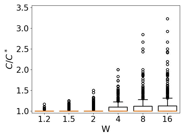
VRP

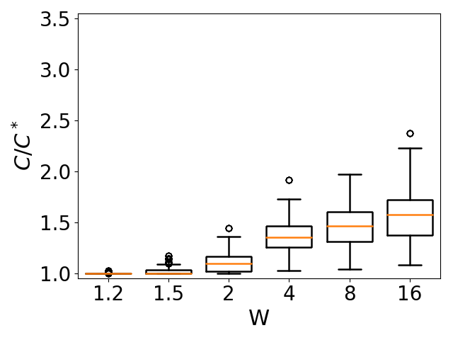
Figure 1: $C/C^{*}$ as a function of $W$ using the Potential heuristic (IPC domains) and for the VRP domain.

Figure 1 shows that Korf’s observations hold across a broad range of domains and heuristics. Boxplots show the distribution of $C/C^{*}$ values for our 568 IPC problems for all values of $W$. This figure is for a specific heuristic – Potential (IPC domains) – and a specific non-IPC domain (VRP). The other $C/C^{*}$ plots are very similar except as noted below. The key features for IPC domains are:

• In all cases at least $25\%$ of the problems are solved optimally.

• For all heuristics except Cegar, the median value of $C/C^{*}$ is 1.0 for all values of $W$. For Cegar, the median is 1.0 for $W=1.2$ and rises very slowly as $W$ increases to a maximum of 1.1 for $W=16$.

• For all values of $W$, $C/C^{*}$ is less than 1.15 on $75\%$ of the problems for all heuristics except for Cegar, for which the $75^{th}$ percentile is 1.3.

• $C/C^{*}$ is almost always less than $\sqrt{W}$. In particular: 73 of the 568 $C/C^{*}$ values are greater than $\sqrt{1.2}$ when $W=1.2$, 47 are greater than $\sqrt{1.5}$ when $W=1.5$, 25 are greater than $\sqrt{2}$ when $W=2$, 8 are greater than $\sqrt{4}$ when $W=4$, 3 are greater than $\sqrt{8}$ when $W=8$, and none is greater than $\sqrt{16}$ when $W=16$.

The results in the non-IPC domains are a bit different than in the IPC domains. The results shown in Figure 1 for VRP are representative of the distributions for the other non-IPC domains, with the 15-puzzle being somewhat worse, and the Pancake puzzle being somewhat better for all of its heuristics. In contrast to the IPC domains, the median, and even the lower quartile (bottom of the boxes), is greater than 1.0 for $W\geq 2$. On the other hand, the largest values of $C/C^{*}$ are smaller in the non-IPC domains than in the IPC domains for all values of $W$.

The observations in these experiments are consistent with Korf’s and others’ (?), and provide compelling evidence that $W$ is a poor estimate of the suboptimality of wA^∗’s solutions, especially when $W$ is large.

5 Why is $W$ a Loose Bound?

Although it is possible to construct examples in which $C/C^{*}=W$, we have just seen that this virtually never happens in practice. In this section, we identify potential causes of this by examining a typical proof that $C/C^{*}\leq W$. This proof uses the fact that, at the beginning of any iteration, for any optimal path $P$ from $start$ to any unclosed state – in particular, any goal state – there exists a node, $n_{opt}\in P$, on $\mathrm{Open}$ such that $g(n_{opt})=g^{*}(n_{opt})$ (Lemma 1 (?)). Then

$f^{W}_{min}$	$\leq\mbox{$f^{W}(n_{opt})$}=g(n_{opt})+Wh(n_{opt})$	(1)
	$=g^{*}(n_{opt})+Wh(n_{opt})$	(2)
	$\leq g^{*}(n_{opt})+Wh^{*}(n_{opt})$	(3)
	$\leq Wg^{*}(n_{opt})+Wh^{*}(n_{opt})$	(4)
	$=W(g^{*}(n_{opt})+h^{*}(n_{opt}))$	(5)
	$=WC^{*}$.

On wA^∗’s final iteration, $f^{W}_{min}$ $=C$, so this derivation establishes that $C/C^{*}\leq W$.

One reason $W$ can overestimate the true value of $C/C^{*}$ is that this derivation applies to $f^{W}_{min}$ on every iteration, it is not specific to the last iteration. A tighter bound on $C/C^{*}$ will almost always be obtained by considering the largest value of $f^{W}_{min}$ that occurred throughout wA^∗’s execution. We call this value $F$. It is easily computed during search and, as we shall see, it can be used to define a much better bound for $C/C^{*}$.

The other sources of potential error (overestimation) in this derivation are the steps that involve an inequality: lines (1), (3), and (4). We do not see any practical way of correcting for the error introduced by line (1), since nodes on an optimal solution path cannot be identified during or even after wA^∗’s search. Furthermore, a step introducing $n_{opt}$ seems inevitable in any derivation of a relation between $C$ and $C^{*}$, since it is via $n_{opt}$ that $C^{*}$ eventually emerges in the derivation.

The error introduced in line (3) is caused by the inaccuracy of the heuristic function $h$. Again, we see no practical way of correcting this error based on the information available during or after wA^∗’s search. And similar to the introduction of $n_{opt}$ in line (1) we see no way of avoiding introducing $h^{*}(n_{opt})$ in deriving a relation between $C$ and $C^{*}$.

The situation is different with the error introduced in line (4). Multiplying $g^{*}(n_{opt})$ by $W$ has no intrinsic justification; it is only done to allow the equation to be simplified. A better way to proceed is as follows (the first few steps are the same as before and are not shown):

$$f^{W}_{min} \leq g^{*}(n_{opt})+Wh^{*}(n_{opt})$$

$$=g^{*}(n_{opt})+W(C^{*}-g^{*}(n_{opt}))$$

$$=WC^{*}-(W-1)g^{*}(n_{opt})$$

$$=WC^{*}-(W-1)g(n_{opt})$$

$$\leq WC^{*}-(W-1)\mbox{$g_{min}$}.$$

This derivation replaces the potentially very large error introduced in the first derivation by multiplying $g^{*}(n_{opt})$ by $W$ with the error seen in the final line: replacing $g(n_{opt})$ by $g_{min}$. In preliminary experiments this error was 0 more than 50% of the time and was rarely a significant fraction of the total error.

As noted above, this derivation is true for $f^{W}_{min}$ on all iterations, and therefore we have

$$F\leq WC^{*}-(W-1)\mbox{$g_{min}$}$$

where $g_{min}$ is the smallest $g$-value on $\mathrm{Open}$ at the beginning of an iteration when a node $n$ with $f^{W}(n)=F$ was removed from $\mathrm{Open}$. It is interesting to see an additive correction term for $F\leq WC^{*}$ that will only be $0$, when $W>1$, in the rare situation that $\mbox{$g_{min}$}=0$. With some simple algebraic rearrangement, this inequality gives the following suboptimality bound for wA^∗, which we call the F bound:

$$\frac{C}{C^{*}}\leq\frac{CW}{F+(W-1)\mbox{$g_{min}$}}.$$

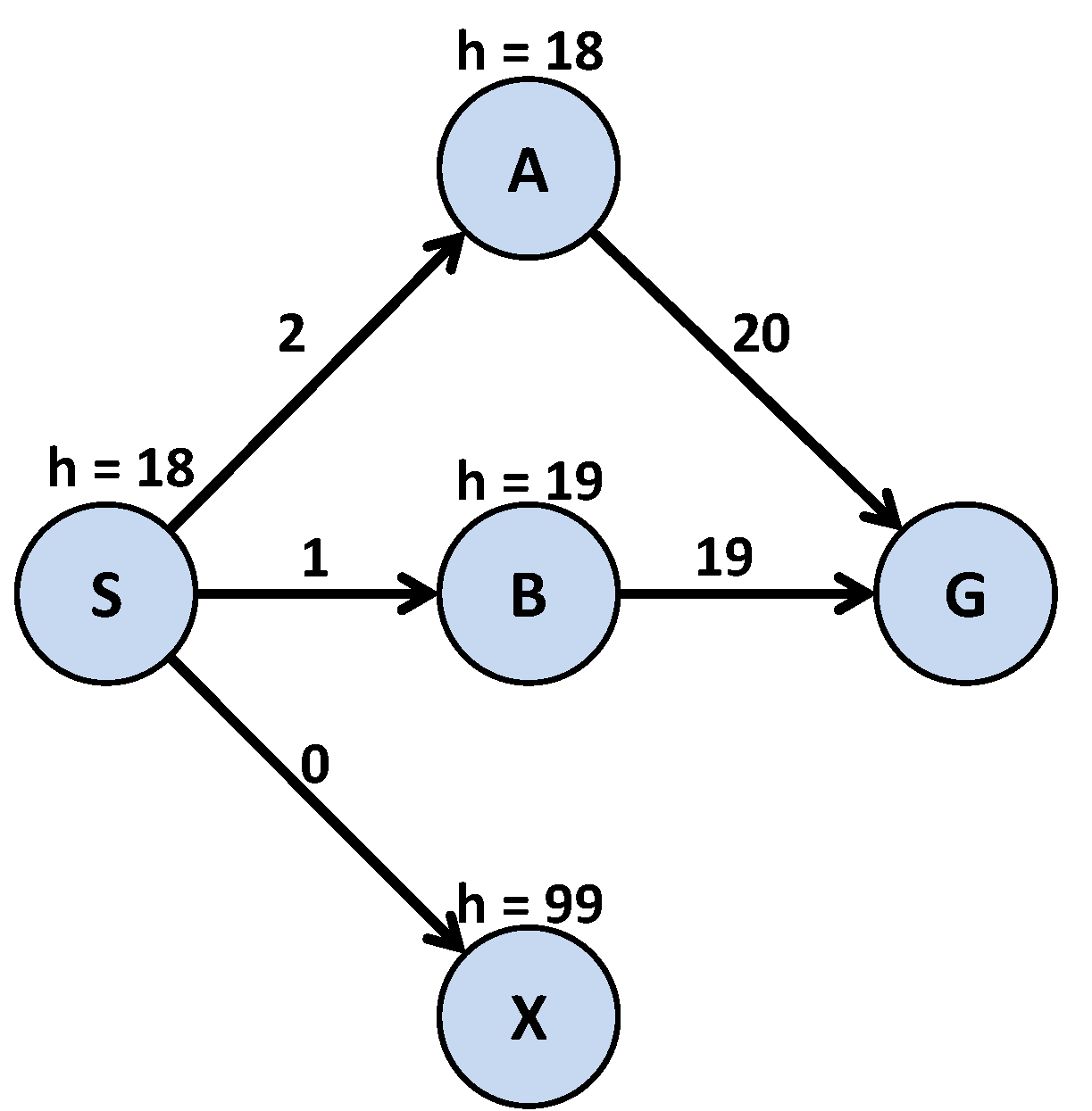
Figure 2: The F bound is a much better bound than $W$.

To see how accurate the F bound can be, consider Figure 2 when $W=10$. The heuristic values here are consistent and $g_{min}$ is $0$ on all iterations. The optimal path is through $B$, and its cost is $C^{*}=20$. $B$’s large $h$-value prevents wA^∗ from expanding $B$ and finding the optimal path. Instead, wA^∗ returns the path through $A$, costing $22$. $F=\max\{f(S),f(A),f(G)\}=182$, so the F bound is $(22\cdot 10)/182=1.2$, which is very close to the actual value of $C/C^{*}$ ($22/20=1.1$) and almost an order of magnitude smaller than $W$. We have experimentally observed that computing the F bound results in a negligible overhead.

6 Experimental Evaluation

The F bound corrects for two sources of overestimation in using $W$ as a bound on $C/C^{*}$. The question addressed by the experiments in this section is, how effective are those corrections? Do they eliminate much of the overestimation? We will answer this question by evaluating the accuracy of the F bound relative to the accuracy of $W$ as an upper bound on $C/C^{*}$.

To quantify the accuracy of the F bound we must take into account how its value, $v_{{\sc F}}$, on a given problem compares to the minimum and maximum possible values on the problem ($C/C^{*}$ and $W$ respectively). We denote the accuracy of the F bound’s value by $\rho$, defined as

$$\rho=\frac{\log(v_{{\sc F}})-\log(C/C^{*})}{\log(W)-\log(C/C^{*})}.$$

The denominator is the distance, in log space, between the F bound’s minimum and maximum possible values, and the numerator is the distance in log space between the F bound’s actual value on a problem ($v_{{\sc F}}$) and its minimum possible value. $\rho$ is always between $0$ and $1$ and represents the F bound’s distance from $C/C^{*}$ as a fraction of $W$’s distance from $C/C^{*}$. A smaller value means better accuracy.

We consider $\rho>0.5$ to be a poor score since it means $v_{{\sc F}}$ is closer to $W$, in log space, than it is to $C/C^{*}$. We consider $\rho\leq 0.25$ to be a good score. For example, if $W=32$ and $C/C^{*}=2$, $v_{{\sc F}}=8$ corresponds to $\rho=0.5$ while $v_{{\sc F}}=4$ corresponds to $\rho=0.25$.

Figure 3 has a boxplot for $\rho$ ($y$-axis) as a function of $W$ ($x$-axis) for the iPDB and Potential heuristics. The results for other heuristics are similar to the iPDB ones, except for the Cost-Partioning heuristic where they are better. The Potential heuristic results are uniformly poorer than the rest. The main trends for all heuristics except for Potential are:

iPDB
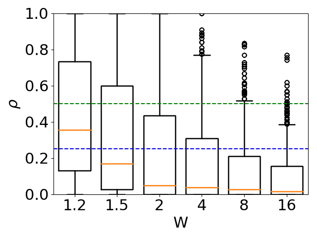
Potential

Figure 3: Boxplots showing the accuracy ($\rho$) on the $y$-axis of the F bound as a function of $W$ ($x$-axis) for the iPDB and Potential heuristics. The horizontal lines that span the entire $x$-axis indicate our thresholds for “good” ($\rho\leq 0.25$) and “bad” ($\rho\geq 0.5$) $\rho$ values.

• The accuracy of the F bound improves as $W$ increases. All aspects of the distribution improve: the median, the $75^{th}$ percentile, (top of the box), the upper whisker, and even the outliers. These all decrease as $W$ increases. This is also true in the non-IPC domains, except for VRP where the distributions only worsen from $W=1.2$ to $W=1.5$.

• In Figure 3 the boxes are seated on $\rho=0$ for $W\geq 2$, meaning the F bound perfectly predicts $C/C^{*}$ for at least $25\%$ of the problems when $W\geq 2$. This holds for all heuristics except Potential. In the non-IPC domains, the F bound does not provide any perfect prediction except for a single Pancake puzzle problem with the GAP heuristic.

• For all heuristics except the Potential heuristic, the median values of the F bound are “good” for all values of $W\geq 2$. When using Cost-Partioning, in 50% of the problems the prediction is perfect when $W\geq 2$. In the non-IPC 15-puzzle and VRP domains, the median values of the F bound are “good” when $W\geq 8$. For the Pancake puzzle the median value is “good” when $W\geq 4$ if the GAP heuristic is used, when $W\geq 8$ if the GAP-1 heuristic is used, and only when $W\geq 16$ if the GAP-2 heuristic is used.

• The distributions are very broad, covering the entire range of possible $\rho$ values for $W\leq 4$. With the Operator-Counting, iPDB, and Cost-Partioning heuristics the $75^{th}$ percentile (top of each box) is a “good” $\rho$ value for larger values of $W$. This is also true in the non-IPC domains for $W=16$. The tails of the distributions stretch into the region of “poor” $\rho$ values for all heuristics and $W$ values in the IPC domains but only when $W\leq 4$ for the non-IPC domains.

7 Conclusions

In this paper we have presented compelling evidence that $W$ is, indeed, almost always a very loose bound on the suboptimality ($C/C^{*}$) of wA^∗’s solutions, especially for larger $W$. We have also identified the causes of this looseness and presented a practical method, the F bound, for correcting for two of them once wA^∗ has finished executing. Finally, we examined how effective these corrections are, i.e. how much more accurately $C/C^{*}$ is predicted by the F bound than by $W$. Our overall conclusion is that the corrections embodied in the F bound are very effective (the F bound predicts $C/C^{*}$ much more accurately than $W$) for any of the heuristics we tested when $W\geq 8$. However, there do exist problems for which the F bound’s predictions are poor, with the number of such problems decreasing as $W$ increases.

We do not claim that the F bound is the best possible post hoc suboptimality bound for wA^∗. Indeed, we know it is not when the heuristic being used is consistent, because we have proven, in that case, that the F bound is dominated by a bound based on the largest unweighted $f$-value on wA^∗’s open list upon termination (see Appendix A). Our aim in introducing the F bound is to show that it is possible to explain, and directly correct for, a great deal of $W$’s looseness as a suboptimality bound for wA^∗.

Appendix A The $\boldsymbol{f}$ bound dominates the $\boldsymbol{F}$ bound when the heuristic is consistent

In this appendix $f_{min}$ refers to the smallest unweighted $f$-value on $Open$ at the beginning of wA^∗’s last iteration, and the $f$ bound is defined to be $C/\mbox{$f_{min}$}$.

Theorem 1.

The $F$ bound is dominated by the $f$ bound if the heuristic is consistent.

Proof: We have to prove that

$$\frac{CW}{F+(W-1)\mbox{$g_{min}$}}\geq C/\mbox{$f_{min}$},$$ (1)

always holds when $h$ is consistent.

Equation 1 is equivalent to

$$W\mbox{$f_{min}$}\geq F+(W-1)\mbox{$g_{min}$}$$ (2)

We observe that $F$ is always equal to the maximum $f^{W}$-value on the solution returned by wA^∗; i.e. if the path returned is $S=s_{0},s_{1},\dots,s_{n}~{}(s_{0}=start,s_{n}$ a goal state$)$ and $F_{S}=\max\{\mbox{$f^{W}(s_{i})$}\}$, then $F=F_{S}$. The reason is the following. $F<F_{S}$ is impossible since all the nodes on $S$ are removed from $\mathrm{Open}$ before termination. $F>F_{S}$ is impossible because at the start of any iteration there is an $s_{i}$ on $\mathrm{Open}$ so $\mbox{$f^{W}_{min}$}\leq F_{S}$ always holds. Therefore, $F=F_{S}$.

Let $m$ be a state on path $S$ with $\mbox{$f^{W}(m)$}=F$, let $n$ be a node on $Open$ at the beginning of wA^∗’s last iteration with $\mbox{$f(n)$}=\mbox{$f_{min}$}$, and let $P$ be the path by which $n$ was placed on $Open$ for the final time (i.e. with $\mbox{$f(n)$}=\mbox{$f_{min}$}$).

Note that, for all states $a$, $W\mbox{$f(a)$}=(W-1)g(a)+\mbox{$f^{W}(a)$}$, so $W\mbox{$f(a)$}\geq\mbox{$f^{W}(a)$}$ if $W>1$.

There are two cases to consider: (1) $m$ is on path $P$, i.e. $n$ is a descendant of $m$; (2) $m$ is not on path $P$.

Case 1. $\boldsymbol{m}$ is on path $\boldsymbol{P}$. In this case, Equation 2 follows directly from the heuristic’s consistency, as follows.

$$h(m) \leq c(m,n)+h(n)$$

$$g(m)+h(m) \leq\mbox{$f(n)$}=\mbox{$f_{min}$}$$

$$Wg(m)+Wh(m) \leq W\mbox{$f_{min}$}$$

$$(W-1)g(m)+g(m)+Wh(m) \leq W\mbox{$f_{min}$}$$

$$(W-1)g(m)+\mbox{$f^{W}(m)$} \leq W\mbox{$f_{min}$}$$

$$(W-1)g(m)+F \leq W\mbox{$f_{min}$}$$

$$(W-1)\mbox{$g_{min}$}+F \leq W\mbox{$f_{min}$}.$$

The last step of the derivation follows from the definition of $g_{min}$ (at the time $m$ was chosen for expansion).

Case 2. $\boldsymbol{m}$ is not on path $\boldsymbol{P}$. This case has two subcases: (a) $n$ was on $\mathrm{Open}$ with $\mbox{$f(n)$}=\mbox{$f_{min}$}$ at the time $m$ was chosen for expansion; (b) $n$ was not on $\mathrm{Open}$ with $\mbox{$f(n)$}=\mbox{$f_{min}$}$ at the time $m$ was chosen for expansion.

Case 2(a). $\boldsymbol{n}$ was on $\boldsymbol{\mathrm{Open}}$ with $\boldsymbol{\mbox{$f(n)$}=\mbox{$f_{min}$}}$ when $\boldsymbol{m}$ was removed from $\boldsymbol{\mathrm{Open}}$. Since $m$ was chosen for expansion, it must be that $\mbox{$f^{W}(n)$}\geq\mbox{$f^{W}(m)$}=F$. Noting that $W\mbox{$f_{min}$}=W\mbox{$f(n)$}=(W-1)g(n)+\mbox{$f^{W}(n)$}\geq(W-1)g(n)+F$ and that $g(n)\geq\mbox{$g_{min}$}$ we get the desired result ($W\mbox{$f_{min}$}\geq F+(W-1)\mbox{$g_{min}$}$).

Case 2(b). $\boldsymbol{n}$ was added to $\boldsymbol{\mathrm{Open}}$ with $\boldsymbol{\mbox{$f(n)$}=\mbox{$f_{min}$}}$ after $\boldsymbol{m}$ was removed from $\boldsymbol{\mathrm{Open}}$. This means some state $x\neq n$ on path $P$ was on $\mathrm{Open}$ at the time $m$ was chosen for expansion (note: $x=m$ is not possible, since in the case we are considering $m$ is not on path $P$). $\mbox{$f^{W}(x)$}>\mbox{$f^{W}(m)$}=F$ is impossible, since $x$ is eventually expanded (in order to complete path $P$) and, by definition of $F$, no state $s$ is ever expanded with $\mbox{$f^{W}(s)$}>F$. $\mbox{$f^{W}(x)$}<\mbox{$f^{W}(m)$}$ contradicts $m$ being chosen for expansion, so at the time $m$ is removed from $\mathrm{Open}$, we must have $\mbox{$f^{W}(x)$}=\mbox{$f^{W}(m)$}=F$. With this equality established, we can now use exactly the same reasoning as we did in Case 1, just substituting $x$ for $m$ everywhere:

$$h(x) \leq c(x,n)+h(n)$$

$$g(x)+h(x) \leq\mbox{$f(n)$}=\mbox{$f_{min}$}$$

… etc. …

$$(W-1)\mbox{$g_{min}$}+F \leq W\mbox{$f_{min}$}.~{}~{}~{}~{}~{}~{}~{}~{}~{}~{}~{}~{}~{}~{}~{}~{}~{}~{}~{}~{}~{}~{}~{}~{}~{}~{}~{}~{}\qed$$

Figure 4 shows that the $f$ bound can be worse than the $F$ bound if the heuristic is even “slightly” inconsistent. $S$ is the start state, $G$ the goal. Consistency requires $h(m)-h(n)\leq 1$, but it is 2. $g_{min}$ is $0$ on all iterations. The optimal solution, $S$–$m$–$n$–$G$, costs $C^{*}=6$. When $W=2$, $\mbox{$f^{W}(n)$}=8$ so wA^∗ returns solution $S$–$m$–$G$ costing $C=7$. $\mbox{$f_{min}$}=\mbox{$f(n)$}=5$ and $F=\mbox{$f^{W}(m)$}=11$. The $F$ bound ($\frac{CW}{F}=\frac{14}{11}$) is strictly smaller than the $f$ bound ($\frac{7}{5}$).

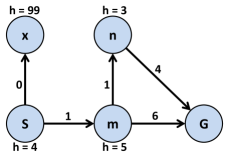
Figure 4: Inconsistent heuristic ($h(m)\nleq c(m,n)+h(n)$).

References

- [Davis, Bramanti-Gregor, and Wang 1988] Davis, H.; Bramanti-Gregor, A.; and Wang, J. 1988. The advantages of using depth and breadth components in heuristic search. In Methodologies for Intelligent Systems, 19–28.
- [Fan, Holte, and Mueller 2018] Fan, G.; Holte, R.; and Mueller, M. 2018. MS-Lite: A lightweight, complementary merge-and-shrink method. In Proc. 28th International Conference on Automated Planning and Scheduling (ICAPS), 74–82.
- [Hart, Nilsson, and Raphael 1968] Hart, P. E.; Nilsson, N. J.; and Raphael, B. 1968. A formal basis for the heuristic determination of minimum cost paths. IEEE Trans. Systems Science and Cybernetics 4(2):100–107.
- [Haslum et al. 2007] Haslum, P.; Botea, A.; Helmert, M.; Bonet, B.; and Koenig, S. 2007. Domain-independent construction of pattern database heuristics for cost-optimal planning. In Proc. 22nd AAAI Conference on Artificial Intelligence, 1007–1012.
- [Helmert and Domshlak 2009] Helmert, M., and Domshlak, C. 2009. Landmarks, critical paths and abstractions: What’s the difference anyway? In Proc. International Conference on Automated Planning and Scheduling (ICAPS).
- [Helmert 2006] Helmert, M. 2006. The Fast Downward planning system. JAIR 26:191–246.
- [Helmert 2010] Helmert, M. 2010. Landmark heuristics for the pancake problem. In Proc. 3rd Annual Symposium on Combinatorial Search, (SoCS).
- [Holte et al. 2016] Holte, R. C.; Felner, A.; Sharon, G.; and Sturtevant, N. R. 2016. Bidirectional search that is guaranteed to meet in the middle. In Proc. 30th AAAI Conference on Artificial Intelligence.
- [Korf 1985] Korf, R. E. 1985. Depth-first iterative-deepening: An optimal admissible tree search. Artificial Intelligence 27(1):97–109.
- [Korf 1993] Korf, R. E. 1993. Linear-space best-first search. Artificial Intelligence 62(1):41–78.
- [Pearl 1984] Pearl, J. 1984. Heuristics – Intelligent Search Strategies for Computer Problem Solving. Addison-Wesley.
- [Pohl 1970] Pohl, I. 1970. Heuristic search viewed as path finding in a graph. Artificial Intelligence 1(3):193–204.
- [Pommerening et al. 2014] Pommerening, F.; Röger, G.; Helmert, M.; and Bonet, B. 2014. LP-Based heuristics for cost-optimal planning. In Proc. 24th International Conference on Automated Planning and Scheduling (ICAPS).
- [Seipp and Helmert 2013] Seipp, J., and Helmert, M. 2013. Counterexample-guided Cartesian abstraction refinement. In Proc. 23rd International Conference on Automated Planning and Scheduling (ICAPS).
- [Seipp, Keller, and Helmert 2017] Seipp, J.; Keller, T.; and Helmert, M. 2017. A comparison of cost partitioning algorithms for optimal classical planning. In Proceedings of ICAPS.
- [Seipp, Pommerening, and Helmert 2015] Seipp, J.; Pommerening, F.; and Helmert, M. 2015. New optimization functions for potential heuristics. In Proc. 25th International Conference on Automated Planning and Scheduling (ICAPS), 193–201.
- [Thayer and Ruml 2008] Thayer, J. T., and Ruml, W. 2008. Faster than weighted A*: An optimistic approach to bounded suboptimal search. In Proc. 18th International Conference on Automated Planning and Scheduling (ICAPS), 355–362.