Modulation-resonance mechanism for
surface waves in a two-layer fluid system

Abstract

We propose a Boussinesq-type model to study the surface/interfacial wave manifestation of an underlying, slowly-varying, long-wavelength, baroclinic flow in a two-layer, density-stratified system. The results of our model show numerically that, under strong nonlinearity, surface waves, with their typical wavenumber being the resonant $k_{\mathrm{res}}$, can be generated locally at the leading edge of the underlying slowly-varying, long-wavelength baroclinic flow. Here, the resonant $k_{\mathrm{res}}$ satisfies the class 3 triad resonance condition among two short-mode waves and one long-mode wave in which all waves propagate in the same direction. Moreover, when the slope of the baroclinic flow is sufficiently small, only one spatially-localized large-amplitude surface wave packet can be generated at the leading edge. This localized surface wave packet becomes high in amplitude and large in group velocity after the interaction with its surrounding waves. These results are qualitatively consistent with various experimental observations including resonant surface waves at the leading edge of an internal wave. Subsequently, we propose a mechanism, referred to as the modulation-resonance mechanism, underlying these surface phenomena, based on our numerical simulations. The proposed modulation-resonance mechanism combines the linear modulation (ray-based) theory for the spatiotemporal asymmetric behavior of surface waves and the nonlinear class 3 triad resonance theory for the energy focusing of surface waves around the resonant wavenumber $k_{\mathrm{res}}$ in Fourier space.

1 Introduction

Large-amplitude internal waves with long wavelengths that propagate over long distances are a universal phenomenon in density-stratified coastal ocean regions, and they play an important role in transferring momentum, heat, and energy in those regions (Alford et al., 2015; Duda & Farmer, 1999, and references therein). Internal waves are not directly visible to observers; their presence can be inferred using the scattering of radar illumination from their accompanying surface waves (SWs). In recent decades, observation data for the surface signature of internal waves have been recorded using Synthetic Aperture Radar (SAR) in many coastal seas worldwide. However, the mechanism underlying the surface signature of internal waves has not been completely understood.

In many field observations, there exists a significant disparity between the typical scales of internal waves and their accompanying SWs: the typical wavelength of internal waves is several kilometres and the typical amplitude is about $100$ metres (Perry & Schimke, 1965; Duda et al., 2004), while on the other hand, the accompanying SWs are between a decimetre and a metre in wavelength (Gargett & Hughes, 1972; Bakhanov & Ostrovsky, 2002; Hwung et al., 2009). A basic surface manifestation of internal waves consists of wide bands of smooth surface (slicks), alternating with narrow bands of rough surface, possibly containing breaking waves (roughness) (Gargett & Hughes, 1972; Alpers, 1985). The typical features of the internal-wave surface signature reported in various field observations can be summarized as follows:

(i) Surface roughness at the leading edge of internal waves: The surface ripples were found to be located at the leading edge of an internal wave (Osborne & Burch, 1980; Alpers, 1985; Gasparovic et al., 1988; Bakhanov & Ostrovsky, 2002; Moore & Lien, 2007). In the narrow rough regions, due to the tendency of SWs to shorten and steepen, they are more likely to break and then leave behind calm water after the internal-wave passage (Phillips, 1966; Gasparovic et al., 1988; Craig et al., 2012).

(ii) Resonant excitations: The rough region travels along with the internal wave; that is, the SW group velocity is close to the internal-wave phase velocity (Osborne & Burch, 1980; Kropfli et al., 1999; Hwung et al., 2009; Craig et al., 2012).

To understand the above two surface phenomena, we numerically study the surface-wave and interfacial-wave (IW) manifestation in a two-layer, density-stratified system using a weakly nonlinear Boussinesq-type model. In this work, we focus on qualitatively capturing the above two phenomena of the surface signature reflecting an underlying IW. Subsequently, we propose a mechanism, referred to as the modulation-resonance mechanism, inferred from our simulation to understand the dynamical behavior of these SWs.

A large volume of literature is dedicated to two-layer fluid systems modeling the interaction between interfacial and surface waves. These works can be broadly grouped into two classes. The first class consists of the literature addressing the linear modulation (or ray-based) theory. These ray-based studies take a statistical viewpoint of SWs modulated by a near-surface current induced by IWs, and invoke phase-averaged models based on a wave-balance equation and ray-based theory (e.g. Gargett & Hughes, 1972; Lewis et al., 1974; Caponi et al., 1988; Bakhanov & Ostrovsky, 2002; Apel et al., 2007; Kodaira et al., 2016). The second class consists of the literature addressing the nonlinear resonance theory, in particular, the class 3 triad resonance theory (Lewis et al., 1974; Hashizume, 1980; Alam, 2012; Craig et al., 2012; Tanaka & Wakayama, 2015). These studies are based on the possibility of a resonant interaction between multiple modes which coexist in a two-layer density-stratified fluid system (Phillips, 1974; Lewis et al., 1974; Benney, 1977). Many of the theoretical studies are dedicated to the effective model describing resonant coupling between interfacial and surface waves, which is derived from two-layer Euler equations using the triad resonance condition via a multi-scale analysis (Lewis et al., 1974; Kawahara et al., 1975; Hashizume, 1980; Funakoshi & Oikawa, 1983; Sepulveda, 1987; Lee et al., 2007; Hwung et al., 2009; Craig et al., 2012). In contrast, only a few of numerical-simulation studies concern the triad resonant phenomena (Funakoshi & Oikawa, 1983; Hwung et al., 2009; Craig et al., 2012; Tanaka & Wakayama, 2015), such as the inverse energy cascade phenomenon for SWs (Tanaka & Wakayama, 2015). However, it is still challenging to simultaneously capture the above surface phenomena (i) and (ii) in these previous theories and numerics.

In this work, we focus on the qualitative behavior of SWs when there is an underlying baroclinic flow, and use numerical simulations to mimic and understand the field observations of (i) surface ripples located at the leading edge and (ii) resonant excitations of these surface ripples. Our two-layer model predicts that, in the strongly nonlinear regime, a finite number of localized SW packets can be generated at the leading edge of the background baroclinic flow (BBF) with their group velocity being close to the phase velocity of the BBF. To examine the robustness of our model results, we investigate the behavior of these SWs for various underlying BBFs in a parametric study. In particular, if the slope of the BBF is sufficiently small, only one localized SW packet or very few localized SW packets can be generated at the leading edge, and they become high in amplitude and large in group velocity after interacting with the surrounding waves.

Importantly, we propose the modulation-resonance mechanism to understand the above surface phenomena. The proposed mechanism combines two different mechanisms: [modulation mechanism] First, based on the linear modulation (ray-based) theory, SW packets propagate quickly towards the leading edge of the BBF and a sink of SW packets is thereafter formed at the leading edge. [resonance mechanism] Subsequently, based on the class 3 triad resonance, the spectrum of SWs can eventually be concentrated near the resonant wavenumber in the wavenumber $k$ space, and simultaneously these resonant SWs become high in amplitude at the leading edge in the spatial domain. The modulation-resonance mechanism may be extended to general density-stratified fluid systems in both shallow-water and deep-water configurations.

The paper is organized as follows. In § 2, we formulate the density-stratified-fluid problem, and provide a weakly-nonlinear Boussinesq-type model describing the coupling between IWs and free SWs. In § 3 and § 4, we numerically investigate the qualitatively-consistent IW surface signatures (i) and (ii) using our model, and further propose the modulation-resonance mechanism underlying these surface manifestations. In § 5, we present conclusions and discussion. We relegate some technical details to the appendices.

2 Formulation of the two-layer fluid system

2.1 The two-layer weakly nonlinear (TWN) model

We begin with Euler equations for two immiscible layers of potential fluids with unequal densities. The fluids in the two layers are assumed to be inviscid, irrotational, and incompressible, with unequal densities, $\rho_{1}$ in the upper layer and $\rho_{2}$ ($>\rho_{1}$ for the stable case) in the lower layer. The horizontal and vertical coordinates are denoted by $x$ and $z$, respectively. The interface and the overlaying free-surface displacements are denoted, respectively, by $\xi_{2}$ and $\xi_{1}$ (see figure 1). The pressure exerted at the surface is denoted by $P_{1}$. Then, the governing equations for the two-layer Euler system are given as follows:

$$\phi_{1xx}+\phi_{1zz}=0,\text{ \ \ }\xi_{2}<z<h_{1}+\xi_{1},$$ (1)

$$\phi_{2xx}+\phi_{2zz}=0,\text{ \ \ }-h_{2}<z<\xi_{2},$$ (2)

$$\xi_{1t}+\phi_{1x}\xi_{1x}=\phi_{1z},\text{ \ \ at }z=h_{1}+\xi_{1},$$ (3)

$$\phi_{1t}+\frac{1}{2}\left(\phi_{1x}^{2}+\phi_{1z}^{2}\right)+g\xi_{1}+P_{1}/\rho_{1}=0,\text{ \ \ at }z=h_{1}+\xi_{1},$$ (4)

$$\xi_{2t}+\phi_{1x}\xi_{2x}=\phi_{1z},\text{ \ \ at }z=\xi_{2},$$ (5)

$$\xi_{2t}+\phi_{2x}\xi_{2x}=\phi_{2z},\text{ \ \ at }z=\xi_{2},$$ (6)

$$\rho_{1}\left(\phi_{1t}+\frac{1}{2}\left(\phi_{1x}^{2}+\phi_{1z}^{2}\right)+g\xi_{2}\right)$$ (7)

$$=\rho_{2}\left(\phi_{2t}+\frac{1}{2}\left(\phi_{2x}^{2}+\phi_{2z}^{2}\right)+g\xi_{2}\right),\text{ \ \ at }z=\xi_{2},$$

$$\phi_{2z}=0,\text{ \ \ at }z=-h_{2},$$ (8)

where $\phi_{1}$ ($\phi_{2}$) is the velocity potential of the upper (lower) fluid layer, $h_{1}$ ($h_{2}$) is the undisturbed thickness of the upper (lower) fluid layer, respectively, and $g$ is the gravitational acceleration.

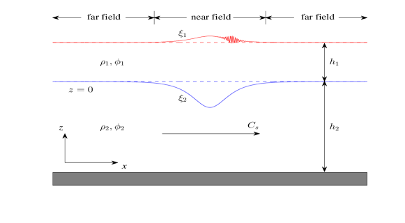
Figure 1: (Colour online) Sketch of the two-layer fluid system. The surface ripples are located at the leading edge of the IW. Near field corresponds to the region near the central IW and far field corresponds to the region far from the central IW.

For the small-amplitude approximation, we assume that the characteristic amplitude, $a$, of the IWs and SWs is much smaller than the thickness of the upper fluid layer,

$$a/h_{1}=\alpha\ll 1.$$ (9)

For the long-wave approximation, we assume that the thickness of each fluid layer is much smaller than the characteristic wavelength, $l$, of the IWs and SWs,

$$h_{1}^{2}/l^{2}=\beta=O(\alpha)\ll 1,\text{\ \ \ }h_{2}=O(h_{1}),$$ (10)

The two small parameters, $\alpha$ and $\beta$, control the nonlinear and dispersive effects, respectively. Based on the scaling (9)-(10), we nondimensionalize all the physical variables in the Euler equations (1)-(8). Next, we apply asymptotic analysis to these nondimensionalized equations, similar to that applied in the derivation of the KdV equation (Whitham, 1974). Retaining the terms in the first power of $\alpha$ and $\beta$, we obtain the set of equations in the dimensional form for the variables $(\xi_{1},\overline{u}_{1},\xi_{2},\overline{u}_{2})$ [to which we refer as the two-layer weakly-nonlinear model or TWN model],

$$\eta_{1t}+(\eta_{1}\overline{u}_{1})_{x}=0,\text{ \ \ }\eta_{1}=h_{1}+\xi_{1}-\xi_{2},$$ (11)

$$\eta_{2t}+(\eta_{2}\overline{u}_{2})_{x}=0,\text{ \ \ }\eta_{2}=h_{2}+\xi_{2},$$ (12)

$$\overline{u}_{1t}+\overline{u}_{1}\overline{u}_{1x}+g\xi_{1x}-\frac{1}{3}h_{1}^{2}\overline{u}_{1xxt}+\frac{1}{2}h_{1}\xi_{2xtt}+P_{1x}/\rho_{1}=0,$$ (13)

$$\overline{u}_{2t}+\overline{u}_{2}\overline{u}_{2x}+g\xi_{2x}+\rho_{r}g\eta_{1x}$$ (14)

$$-\frac{1}{2}\rho_{r}h_{1}^{2}\overline{u}_{1xxt}+\rho_{r}h_{1}\xi_{2xtt}-\frac{1}{3}h_{2}^{2}\overline{u}_{2xxt}+P_{1x}/\rho_{2}=0,$$

where $\rho_{r}$ is the density ratio $\rho_{1}/\rho_{2}$, and

$$\overline{u}_{1}(x,t)=\dfrac{1}{\eta_{1}}\int_{\xi_{2}}^{h_{1}+\xi_{1}}\phi_{1x}(x,z,t)dz,\text{ \ \ }\overline{u}_{2}(x,t)=\dfrac{1}{\eta_{2}}\int_{-h_{2}}^{\xi_{2}}\phi_{2x}(x,z,t)dz,$$

are the depth-averaged horizontal velocities of the upper and lower fluid layers, respectively. This weakly-nonlinear model can also be obtained via a direct reduction from a fully nonlinear model given in Choi & Camassa (1996), Barros & Gavrilyuk (2007), and Barros & Choi (2009). We refer to the fully nonlinear model as the MCC model. We provide the dimensionless form of the TWN model in appendix A. Next, we study the basic properties of the TWN model, including the dispersion relation and the class 3 triad resonance condition.

The TWN system admits a linear dispersion relation corresponding to a monochromatic wavetrain with infinitesimal amplitude. By substituting the monochromatic solutions $(\xi_{j},\overline{u}_{j})\sim\exp[\text{i}(kx-\mu_{k}t)]$, $j=1,2$, into the TWN system, we obtain the pure linear dispersion relation between the frequency $\mu_{k}$ and the wavenumber $k$ as

$$\left(1+\rho_{r}k^{2}h_{1}h_{2}+\frac{1}{3}k^{2}h_{1}^{2}+\frac{1}{3}k^{2}h_{2}^{2}+\frac{1}{9}k^{4}h_{1}^{2}h_{2}^{2}+\frac{1}{12}\rho_{r}k^{4}h_{1}^{3}h_{2}\right)\mu_{k}^{4}$$ (15)

$$-\left(gh_{1}+gh_{2}+\frac{1}{3}gk^{2}h_{1}h_{2}^{2}+\frac{1}{3}gk^{2}h_{1}^{2}h_{2}\right)k^{2}\mu_{k}^{2}+\left(1-\rho_{r}\right)g^{2}k^{4}h_{1}h_{2}=0.$$

The same dispersion relation can be found in Barros & Gavrilyuk (2007). Equation (15) always has $4$ real roots when the problem is considered in the oceanic regime, i.e., when the density ratio $\rho_{r}$ is close to $1$. Then, at the leading order in $1-\rho_{r}$, we can approximate the dispersion relation of the two-mode waves, denoted by $\Omega_{k}$ and $\omega_{k}$ [figure 2(a)], as

$$\Omega_{k}^{2}=\frac{\left(1-\rho_{r}\right)g^{2}h_{1}h_{2}k^{2}}{gh_{1}+gh_{2}+\frac{1}{3}gk^{2}h_{1}h_{2}^{2}+\frac{1}{3}gk^{2}h_{1}^{2}h_{2}},$$ (16)

and

$$\omega_{k}^{2}=\frac{\left(gh_{1}+gh_{2}+\frac{1}{3}gk^{2}h_{1}h_{2}^{2}+\frac{1}{3}gk^{2}h_{1}^{2}h_{2}\right)k^{2}}{1+\rho_{r}k^{2}h_{1}h_{2}+\frac{1}{3}k^{2}h_{1}^{2}+\frac{1}{3}k^{2}h_{2}^{2}+\frac{1}{9}k^{4}h_{1}^{2}h_{2}^{2}+\frac{1}{12}\rho_{r}k^{4}h_{1}^{3}h_{2}}.$$ (17)

In the following, the two kinds of waves, corresponding to the dispersion relations $\Omega_{k}$ [equation (16)] and $\omega_{k}$ [equation (17)], are referred to as the long-mode (baroclinic) waves and the short-mode (barotropic) waves, respectively.

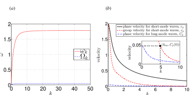
Figure 2: (Colour online) (a) Pure linear dispersion relations $\omega_{k}$ and $\Omega_{k}$ of short-mode waves and long-mode waves, respectively. (b) Comparison of the phase velocity for the short-mode waves $c_{p}$ (solid line ———), the group velocity for the short-mode waves $c_{g}$ (dashed line –  –  –), and the phase velocity for the long-mode waves $C_{p}$ (dashed-dotted line – $\cdot$ – $\cdot$ –). The resonant wavenumber $k_{\mathrm{res}}$ satisfies the triad resonance condition (19). For our simulations in figures 2–9, the parameters are $(h_{1},h_{2},g,\rho_{1},\rho_{2})=(1,3,1,1,1.003)$.

Resonant interactions among different modes are an important process of energy exchange. For the two-mode waves in equations (16) and (17), we can numerically verify the existence of solutions to the class 3 triad resonance condition. If the dispersion relations allow the wavenumbers $k_{j}(j=1,2,3)$ and the frequencies $\omega_{k}(k_{1})$, $\omega_{k}(k_{2})$, and $\Omega_{k}(k_{3})$ to satisfy the condition

$$k_{1} =k_{2}+k_{3},$$ (18)

$$\omega_{k}(k_{1}) =\omega_{k}(k_{2})+\Omega_{k}(k_{3}),$$

the corresponding three waves constitute a class 3 resonant triad. Moreover, if the wavenumbers have the specific form $k_{1}=k_{\text{res}}+\Delta k/2$, $k_{2}=k_{\text{res}}-\Delta k/2$, $k_{3}=\Delta k$, where $\Delta k\ll k_{\text{res}}$ and $\Delta k\rightarrow 0$, then the resonance condition reduces to

$$c_{g}(k_{\text{res}})=C_{p}(0),$$ (19)

where the group velocity $c_{g}$ and the phase velocity $C_{p}$ are given by the equations

$$c_{g}(k_{\text{res}})\equiv\left.\frac{\partial\omega_{k}}{\partial k}\right|_{k=k_{\text{res}}},\ \ C_{p}(0)\equiv\left.\frac{\Omega_{k}(\Delta k)}{\Delta k}\right|_{\Delta k\rightarrow 0}.$$ (20)

Here, $k_{\text{res}}$ is referred to as the resonant wavenumber. Many early results (Phillips, 1974; Hashizume, 1980; Craig et al., 2011, 2012) have confirmed that there exists a unique resonant wavenumber $k_{\text{res}}$ satisfying equation (19) in the two-layer system. The resonance condition (19) shows that, for resonantly-interacting waves, the group velocity of short-mode waves and the phase velocity of long-mode waves are equal (Phillips, 1974; Hashizume, 1980; Craig et al., 2011, 2012). Figure 2(b) shows the phase velocity of the short-mode waves $c_{p}=\omega_{k}/k$, the group velocity of the short-mode waves $c_{g}$, and the phase velocity of the long-mode waves $C_{p}=\Omega_{k}/k$. It can be seen from the inset of figure 2(b) that there indeed exists a resonant wavenumber $k_{\text{res}}$, satisfying the resonance condition (19), $c_{g}(k_{\text{res}})=C_{p}(0)$. Thus, class 3 resonant triads exist among two short-mode waves and one long-mode wave for the TWN model. Note that the class 3 triad resonance condition (18) or (19) is not assumed during the derivation of the TWN model. Nevertheless, the resonance condition (18) from Alam (2012) can be satisfied using the dispersion relations (16) and (17) in the TWN model. As discussed in §§ 3.2, the class 3 triad resonance phenomena will be numerically investigated in our model in detail.

In our numerical simulations, throughout the text, the variables are all dimensionless. That is, numerically, the characteristic length in both height and wavelength is $h_{1}$, the characteristic speed is $\sqrt{gh_{1}}$, and the characteristic time is $\sqrt{h_{1}/g}$ [see similar dimensionless forms used in numerical simulations in (Choi & Camassa, 1999; Choi et al., 2009)]. In this work, two parameter regimes are used in our simulations, one being $(h_{1},h_{2},g,\rho_{1},\rho_{2})=(1,3,1,1,1.003)$ and the other being $(h_{1},h_{2},g,\rho_{1},\rho_{2})=(1,5,1,0.856,0.996)$.

2.2 Modified two-layer weakly nonlinear (mTWN) model

Next, we propose a modified version of the TWN model, which takes into account the effects of a background baroclinic flow. The basic idea is that we are given a slowly-varying, sufficiently-long-wavelength background baroclinic flow (BBF), and then study the behavior of short-mode surface waves on top of this BBF (more details concerning using the BBF can be found in appendix A). We construct the modified model for the effects of the BBF on the propagation of short-mode waves, based on the following assumptions: The long-wave approximation (10) is only applied to the short-mode (barotropic) waves of IWs and SWs. The characteristic wavelength of short-mode waves, $l$, is much shorter than the wavelength of the BBF, $L$,

$$2\pi l/L=\gamma\rightarrow 0.$$ (21)

The displacements associated with the BBF at the interface and at the surface are denoted by $\Xi_{2}^{\ast}$ and $\Xi_{1}^{\ast}$, respectively. The depth-averaged horizontal currents of the upper and lower layers are denoted by $\overline{U}_{1}^{\ast}$ and $\overline{U}_{2}^{\ast}$, respectively. In the rest of the paper, the vector $(\Xi_{j}^{\ast},\overline{U}_{j}^{\ast})$ is referred to as the BBF. The slowly-varying long-wavelength BBF disperses weakly, and thereafter the displacements and currents associated with the BBF, $\Xi_{j}^{\ast}$ and $\overline{U}_{j}^{\ast}$, can be expressed as the right-moving traveling wave $\Xi_{j}^{\ast}(\cdot)=\Xi_{j}^{\ast}\left(K\left(x-C_{s}t\right)\right)$ and $\overline{U}_{j}^{\ast}(\cdot)=\overline{U}_{j}^{\ast}\left(K\left(x-C_{s}t\right)\right)$, where $K=2\pi/L$ is the characteristic wavenumber and $C_{s}$ is the constant phase velocity of the BBF. The BBF, $(\Xi_{j}^{\ast},\overline{U}_{j}^{\ast})$, satisfies the sign constraint $\Xi_{1}^{\ast}>0$, $\Xi_{2}^{\ast}<0$, $\overline{U}_{1}^{\ast}>0$, and $\overline{U}_{2}^{\ast}<0$. The variables $(\xi_{j},\overline{u}_{j})$ in the TWN model eventually will be represented as a sum of two components, one being the BBF, $(\Xi_{j}^{\ast},\overline{U}_{j}^{\ast})$, and the other the perturbations of the waves, $(\xi_{j}^{\ast},\overline{u}_{j}^{\ast})$. We study the motion of the perturbation waves $(\xi_{j}^{\ast},\overline{u}_{j}^{\ast})$, in particular, we focus on the dynamical behavior of IWs and SWs on the BBF. The assumption (21) adopted here is similar to the one adopted in (Hwung et al., 2009). By substituting $(\xi_{j},\overline{u}_{j})=(\Xi_{j}^{\ast},\overline{U}_{j}^{\ast})+(\xi_{j}^{\ast},\overline{u}_{j}^{\ast})$ into the TWN system, applying asymptotic analysis [see appendix A for details], and casting the system in the conservation form in the right-moving frame with velocity $C_{s}$, we obtain the effective evolution equations for the perturbations of waves $(\xi_{j}^{\ast},\overline{u}_{j}^{\ast})$ on the BBF in dimensional form as follows [referred to as modified two-layer weakly nonlinear model or mTWN model]:

$$\eta_{1T}^{\ast}-C_{s}\eta_{1X}^{\ast}+(H_{1}^{\ast}\overline{u}_{1}^{\ast}+\overline{U}_{1}^{\ast}(\xi_{1}^{\ast}-\xi_{2}^{\ast})+\vartheta^{\ast}(\xi_{1}^{\ast}-\xi_{2}^{\ast})\overline{u}_{1}^{\ast})_{X}=0,$$ (22)

$$\eta_{2T}^{\ast}-C_{s}\eta_{2X}^{\ast}+(H_{2}^{\ast}\overline{u}_{2}^{\ast}+\overline{U}_{2}^{\ast}\xi_{2}^{\ast}+\vartheta^{\ast}\xi_{2}^{\ast}\overline{u}_{2}^{\ast})_{X}=0,$$ (23)

$$M_{1T}^{\ast}-C_{s}M_{1X}^{\ast}+\left(\overline{U}_{1}^{\ast}\overline{u}_{1}^{\ast}+g\xi_{1}^{\ast}+\frac{1}{2}\vartheta^{\ast}\overline{u}_{1}^{\ast 2}\right)_{X}+P_{1X}/\rho_{1}=0,$$ (24)

$$M_{2T}^{\ast}-C_{s}M_{2X}^{\ast}+\left(\overline{U}_{2}^{\ast}\overline{u}_{2}^{\ast}+g\xi_{2}^{\ast}+\rho_{r}g\eta_{1}^{\ast}+\frac{1}{2}\vartheta^{\ast}\overline{u}_{2}^{\ast 2}\right)_{X}+P_{1X}/\rho_{2}=0.$$ (25)

Here

$$H_{1}^{\ast}=h_{1}+\Xi_{1}^{\ast}-\Xi_{2}^{\ast},\text{ \ \ }H_{2}^{\ast}=h_{2}+\Xi_{2}^{\ast},$$

$$\eta_{1}^{\ast}=h_{1}+\xi_{1}^{\ast}-\xi_{2}^{\ast},\text{ \ \ }\eta_{2}^{\ast}=h_{2}+\xi_{2}^{\ast},$$

$$M_{1}^{\ast}=\overline{u}_{1}^{\ast}-\frac{1}{3}h_{1}^{2}\overline{u}_{1XX}^{\ast}-\frac{1}{2}h_{1}\left(H_{2}^{\ast}\overline{u}_{2}^{\ast}+\overline{U}_{2}^{\ast}\xi_{2}^{\ast}+\vartheta^{\ast}\overline{u}_{2}^{\ast}\xi_{2}^{\ast}\right)_{XX},$$

$$M_{2}^{\ast}=\overline{u}_{2}^{\ast}-\frac{1}{2}\rho_{r}h_{1}^{2}\overline{u}_{1XX}^{\ast}-\frac{1}{3}h_{2}^{2}\overline{u}_{2XX}^{\ast}-\rho_{r}h_{1}\left(H_{2}^{\ast}\overline{u}_{2}^{\ast}+\overline{U}_{2}^{\ast}\xi_{2}^{\ast}+\vartheta^{\ast}\overline{u}_{2}^{\ast}\xi_{2}^{\ast}\right)_{XX},$$

and the right-moving frame corresponds to the variable transformation $T=t$ and $X=x-C_{s}t$, where $C_{s}$ is the phase velocity of the BBF $(\Xi_{j}^{\ast},\overline{U}_{j}^{\ast})$, and $P_{1}$ is the normal pressure exerted at the surface. The parameter $\vartheta^{\ast}$ takes two values 1 or 0, where $\vartheta^{\ast}=0$ corresponds to the linear regime and $\vartheta^{\ast}=1$ corresponds to the nonlinear regime for the perturbation waves $(\xi_{j}^{\ast},\overline{u}_{j}^{\ast})$. In the right-moving frame, the BBF $(\Xi_{j}^{\ast},\overline{U}_{j}^{\ast})$ is steady with respect to time $T$. More details concerning the dimensionless form of the mTWN model can be found in appendix A.

3 Review of linear modulation theory and nonlinear class 3 triad resonance

3.1 Linear modulation (or ray-based) theory

In this section, we review the linear modulation (or ray-based) theory for short-mode SWs on a BBF. We take the components of the long-wavelength BBF, $(\Xi_{1}^{\ast},\Xi_{2}^{\ast},\overline{U}_{1}^{\ast},\overline{U}_{2}^{\ast})$, to be proportional to

$$\left\{\tanh\left[s_{\Xi^{\ast}}\left(X+X_{\Xi^{\ast}}\right)\right]-\tanh\left[s_{\Xi^{\ast}}\left(X-X_{\Xi^{\ast}}\right)\right]\right\}/2,$$ (26)

with the maximal amplitudes of $(\Xi_{1}^{\ast},\Xi_{2}^{\ast},\overline{U}_{1}^{\ast},\overline{U}_{2}^{\ast})$ being $(0.0003,-0.1,0.007,-0.006)$, the slope $s_{\Xi^{\ast}}=0.2$, the wavelength $X_{\Xi^{\ast}}=120$, and the phase velocity $C_{s}=0.0485$. Here, the maximal amplitudes and the phase velocity are chosen to be close to those of the interfacial solitary wave solution of the TWN model for $\Xi_{2}^{\ast}(0)=-0.1$ [see appendix B]. The parameter $X_{\Xi^{\ast}}=120$ characterizes the wavelength of the BBF and is chosen to be large enough to satisfy the assumption (21). The parameter $s_{\Xi^{\ast}}$ characterizes the slope of the BBF. Later on in §§ 4.2, we will vary these parameters for a parametric study and see how their values affect the dynamical behavior of short-mode SWs.

In the presence of the baroclinic flow in the right-moving frame, the modulated dispersion relation $\overline{\nu}_{k}$ for the perturbation waves $(\xi_{j}^{\ast},\overline{u}_{j}^{\ast})$ can be obtained by substituting $(\xi_{j},\overline{u}_{j})\sim(\Xi_{j}^{\ast},\overline{U}_{j}^{\ast})+\exp[\text{i}(kX-\overline{\omega}_{k}T)]$ with $\overline{\omega}_{k}=\overline{\nu}_{k}+C_{s}k$ into the TWN system . Here, $\overline{\omega}_{k}$ is the dispersion relation in the resting frame, whereas $\overline{\nu}_{k}$ is the dispersion relation in the right-moving frame. The resulting equation is

$$\left|\begin{array}[]{cccc}\begin{smallmatrix}-\overline{\omega}_{k}+k\overline{U}_{1}^{\ast}&\overline{\omega}_{k}-k\overline{U}_{1}^{\ast}&kh_{1}+k\Xi_{1}^{\ast}-k\Xi_{2}^{\ast}&0\\ 0&-\overline{\omega}_{k}+k\overline{U}_{2}^{\ast}&0&kh_{2}+k\Xi_{2}^{\ast}\\ gk&-\frac{1}{2}kh_{1}\overline{\omega}_{k}^{2}&-\overline{\omega}_{k}-\frac{1}{3}k^{2}h_{1}^{2}\overline{\omega}_{k}+k\overline{U}_{1}^{\ast}&0\\ \rho_{r}gk&(1-\rho_{r})gk-\rho_{r}kh_{1}\overline{\omega}_{k}^{2}&-\frac{1}{2}\rho_{r}k^{2}h_{1}^{2}\overline{\omega}_{k}&-\overline{\omega}_{k}-\frac{1}{3}k^{2}h_{2}^{2}\overline{\omega}_{k}+k\overline{U}_{2}^{\ast}\end{smallmatrix}&&&\end{array}\right|=0,$$ (27)

where $\left|\cdot\right|$ denotes the determinant of the enclosed matrix. Moreover, we also obtain three linear eigenfunction relations among the amplitudes of $(\xi_{j}^{\ast},\overline{u}_{j}^{\ast})$. We note that, first, $(\Xi_{j}^{\ast},\overline{U}_{j}^{\ast})$ are steady in time $T$ in the right-moving frame, so that the dispersion relation $\overline{\nu}_{k}$ is independent of time $T$. Second, the wavelengths of $(\Xi_{j}^{\ast},\overline{U}_{j}^{\ast})$ are relatively long compared to the characteristic length of the short-mode waves, so $(\Xi_{j}^{\ast},\overline{U}_{j}^{\ast})$ in the dispersion relation (27) can be locally treated as constant in $X$ space. Third, if $(\Xi_{j}^{\ast},\overline{U}_{j}^{\ast})=0$, the modulated dispersion relation $\overline{\omega}_{k}$ in equation (27) reduces to the pure linear dispersion relation $\mu_{k}$ in equation (15).

Due to the slow variation in space and time of the phase of the short-mode waves, the governing equations of the space-time rays at the location $X$ and wavenumber $k$ are given by the ray-based theory (Whitham, 1974; Bakhanov & Ostrovsky, 2002; Kodaira et al., 2016),

$$\frac{dX}{dT}=\frac{\partial\overline{\nu}_{k}}{\partial k},$$ (28)

$$\frac{dk}{dT}=-\frac{\partial\overline{\nu}_{k}}{\partial X},$$ (29)

where $\overline{\nu}_{k}$ is the modulated dispersion relation in equation (27). Since the dispersion relation $\overline{\nu}_{k}$ does not explicitly depend on time $T$, equations (28) and (29) constitute a Hamiltonian system with $\overline{\nu}_{k}$ as the Hamiltonian, $X$ displacement, and $k$ momentum. Equation (28) states that the wave packet propagates with the group velocity.

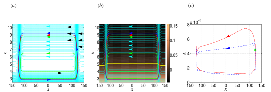
Figure 3: (Colour online) (a) The phase portrait of the right-moving wave-packet motion in the variables $X$ and $k$. Along each cyan-colored curve, the frequency $\overline{\nu}_{k}$ remains constant. Inside the region enclosed by the blue level-curve, the right-moving short-mode waves are trapped. The red level-curve corresponds to the simulation in panel (c). Along the two green level-curves, the minimal wavenumbers are $k=3$ and $k=4$, respectively [corresponding to the initial perturbation (33) in the next § 4]. The arrows indicate the direction of wave-packet movement. (b) Plotted is the group velocity $\partial\overline{\nu}_{k}/{\partial k}$ with its magnitude color-coded [copper-black] on the background. The yellow curve corresponds to zero group velocity. (c) The maximal amplitude $A$ versus the peak location $X$ for the evolution of a narrow wave packet with a narrow band of wavenumbers. The initial value is marked by the green cross. The red curve corresponds to the first period and the blue curve corresponds to the second period. The main observation is that SWs become high at the leading edge, $100<X<120$, and low at the trailing edge, $-120<X<-100$ (asymmetric behavior [1c]). This main observation of asymmetric behavior [1c] persists for both periods (red and blue curves). On the flat BBF ($-100<X<100$), as a result of the wave dispersion, the initially narrow SW packet becomes smaller in maximal amplitude and wider in length. Also, due to the wave dispersion, the maximal amplitude in the second period (blue curve) becomes smaller than that in the first period (red curve). In fact, eventually the waves will be almost uniformly distributed on the flat BBF after several periods [not shown here] due to the wave dispersion and the periodic motion of SWs.

We first study the dynamical behavior of right-moving (positive phase velocity) short-mode SWs. In figure 3(a), the phase portrait of the right-moving wave-packet motion in the variables $X$ and $k$ is constructed from the modulated dispersion relation $\overline{\nu}_{k}$ using the ray-based theory. It can be seen from figure 3(a) that right-moving short-mode waves become short in wavelength at the leading edge ($X>0$), whereas they become long at the trailing edge ($X<0$). Figure 3(b) displays the group velocity of these short-mode waves, $\partial\overline{\nu}_{k}/\partial k$, (in variables $X$ and $k$) with its magnitude color-coded on top of the background. It can be seen from figure 3(b) that, above the yellow curve, $\partial\overline{\nu}_{k}/\partial k<0$ and its absolute value is relatively small, whereas below the yellow curve, $\partial\overline{\nu}_{k}/\partial k>0$ and its absolute value is relatively large. This suggests that the right-moving short-mode wave packets propagate towards the trailing edge [in the direction of decreasing $X$ when $C_{s}>0$] with a relatively small group velocity, and towards the leading edge [in the direction of increasing $X$ when $C_{s}>0$] with a relatively large group velocity.

We now study the relation between the maximal amplitude $A$ and the peak location $X$ of the right-moving short-mode waves. We numerically simulate the mTWN model with $\vartheta^{\ast}=1$ and $P_{1}=0$ in the weakly nonlinear regime. Here, the weakly nonlinear regime means that the amplitude of initial perturbation $(\xi_{j}^{\ast},\overline{u}_{j}^{\ast})$ is very small. The initial perturbation for short-mode waves is a narrow wave packet with a disturbance of a narrow band of wavenumbers. The initial perturbation of $\xi_{2}^{\ast}$ is taken to be

$$\xi_{2}^{\ast}=A_{\varepsilon}[\tanh(X-X_{0}+x_{0})-\tanh(X-X_{0}-x_{0})]\cos(k_{0}(X-X_{0})),$$ (30)

with $A_{\varepsilon}=2\times 10^{-4}$, $X_{0}=123$, $x_{0}=3$ and $k_{0}=5$. This initial perturbation $(X_{0},k_{0})$ is located on the red-level curve in figure 3(a). To allow for only right-moving short-mode waves in the system, the other three variables, $(\xi_{1}^{\ast},\overline{u}_{1}^{\ast},\overline{u}_{2}^{\ast})$, have the same form as the perturbation (30), with their amplitudes satisfying the linear eigenfunction relations following from the matrix in equation (27). For example, we can obtain from the matrix in equation (27) that $\overline{u}_{2}^{\ast}=\left(\overline{\omega}_{k}-k\overline{U}_{2}^{\ast}\right)\xi_{2}^{\ast}/\left(kh_{2}+k\Xi_{2}^{\ast}\right)$. More details about the settings of the numerical simulations, including the numerical scheme, dealiasing strategy, boundary conditions, and Kelvin-Helmholtz instability are presented in appendix C.

Figure 3(c) displays the maximal amplitude $A$ versus the peak location $X$ for the evolution of the perturbation for the right-moving short-mode waves. It can be seen that SWs become high in amplitude at the leading edge ($X>0$) and low at the trailing edge ($X<0$). Notice that this assertion is also true for the Euler system of equations (Lewis et al., 1974). In particular, this SWs’ amplitude phenomenon can be inferred from the energy conservation equation of the Euler system. The energy conservation equation can be obtained using the concept of radiation stress for the Euler system (Lewis et al., 1974):

$$\frac{\partial\widetilde{A}^{2}}{\partial t}+\frac{\partial\left[\left(\widetilde{C}_{g}+\widetilde{U}\right)\widetilde{A}^{2}\right]}{\partial x}=-\frac{1}{2}\widetilde{A}^{2}\frac{\partial\widetilde{U}}{\partial x},$$ (31)

where $\widetilde{C}_{g}$ is the group velocity in the pure linear dispersion relation, $\widetilde{A}$ is the amplitude of SW packets, and $\widetilde{U}$ is the surface-current elevation. At the leading edge, a negative strain rate $\partial\widetilde{U}/\partial x$ corresponds to the growth of the amplitude [surface convergence], whereas at the trailing edge, a positive strain rate $\partial\widetilde{U}/\partial x$ corresponds to the decay of the amplitude [surface divergence].

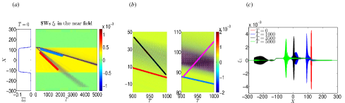
Figure 4: (Colour online) (a) The snapshot of the BBF (left panel) and the spatiotemporal evolution of SWs’ profile $\xi_{1}$. The red and blue lines correspond to the group velocities of the left-moving SWs and right-moving SWs, respectively. (b) Zoomed-in version of (a). The red and blue lines are the same as those in (a). The black and magenta lines correspond to the phase velocities of the left-moving SWs and right-moving SWs, respectively. Note that the phase velocity of the left-moving SWs [black line] is negative whereas the phase velocity of the right-moving SWs [magenta line] is positive. (c) Snapshots of SWs’ profile $\xi_{1}$. Initially at $T=0$ (red curve), there is only a narrow wave packet of SWs. At $T=1000$, the smaller-amplitude left-moving SW packet (blue curve for $X<50$) and the larger-amplitude right-moving SW packet (blue curve for $X>50$) can be seen. Note that the left-moving SW packet, corresponding to a negative phase velocity, is not trapped in the near field. On the other hand, the right-moving SW packet, corresponding to a positive phase velocity, is trapped in the near field. At $T=3500$, the left-moving waves (black curve for $X<-150$) are partially absorbed by the boundary condition [see appendix C]. At $T=5000$, the left-moving waves (green curve for $X<-150$) are completely absorbed by the boundary. For the right-moving waves, as a result of the wave dispersion, the initially narrow SW packet (red curve for $X>100$) becomes smaller in maximal amplitude and wider in length (e.g., green curve for $X>-50$).

Next, we study the dynamical behavior of left-moving (negative phase velocity) short-mode SWs. Figure 4(a) displays the spatiotemporal evolution of SWs’ profile $\xi_{1}$. The initial perturbation of $\xi_{1}^{\ast}$ is the same as that of $\xi_{1}^{\ast}$ used in figure 3(c). However, the initial perturbations of the other three variables, $\xi_{2}^{\ast},u_{1}^{\ast},u_{2}^{\ast}$, are all taken to be zero. It can be seen that the initial narrow wave packet splits into two wave packets, one corresponding to the right-moving SW packet [blue line] and the other corresponding to the left-moving SW packet [red line]. The right-moving waves are trapped in the near field as discussed above and shown in figure 3. On the other hand, the left-moving waves quickly leave the near field [figure 4], and then these left-moving waves are absorbed by the boundary [figures 4(a) and (c)].

To summarize, the behavior of the short-mode waves is asymmetric at the leading edge vs. the trailing edge when there is an underlying BBF:

[1a] Right-moving SW packets propagate towards the trailing edge with a relatively small group velocity, and towards the leading edge with a relatively large group velocity [figure 3(b)].

[1b] Right-moving SWs become short in wavelength at the leading edge and long at the trailing edge [figure 3(a)].

[1c] Right-moving SWs become high in amplitude at the leading edge and low at the trailing edge [figure 3(c)].

[1d] Left-moving SWs quickly leave the near field, and then only the right-moving SWs that propagate in the same direction as the BBF remain trapped in the near field [figure 4].

To the best of our knowledge, the asymmetric behavior [1b] and [1d] was earlier discovered in references (Bakhanov & Ostrovsky, 2002; Kodaira et al., 2016), the asymmetric behavior [1c] was earlier discovered in reference (Lewis et al., 1974), but the asymmetric behavior [1a] was not pointed out earlier. Here, we review these asymmetric types of behavior predicted by the ray-based theory using the mTWN model in the weakly nonlinear regime. These asymmetric types of behavior are important for demonstrating the modulation-resonance mechanism, as will be discussed in § 4 below.

In the rest of the paper, we always use short-mode SWs to denote right-moving short-mode SWs that are trapped in the near field. Whenever we discuss left-moving short-mode SWs, we will directly use the phrase left-moving short-mode SWs.

3.2 Nonlinear class 3 triad resonance

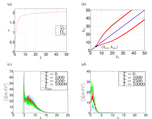
Figure 5: (Colour online) (a) Modulated dispersion relations (27) for the short-mode waves, $\overline{\omega}_{k}$, and the long-mode waves, $\overline{\Omega}_{k}$. (b) The wavenumbers of two short-mode waves satisfying the class 3 triad resonance condition as in equation (18) but using the modulated dispersion relations. Panels (c) and (d) show the evolution of the wavenumber spectra of the SWs $\xi_{1}^{*}$ and the IWs $\xi_{2}^{*}$. The resonant wavenumber is $k_{\mathrm{res}}=5.0$.

In this section, we review the phenomena associated with the nonlinear class 3 triad resonance for short-mode SWs. Class 3 triad resonance is considered responsible for the surface signature of the underlying internal waves. The resonant excitation of surface waves whose group velocity is close to the phase velocity of long internal waves has been reported in various observations (Lewis et al., 1974; Osborne & Burch, 1980). Many works have been dedicated to the effective model describing class 3 triad-resonance coupling phenomena between interfacial and surface waves using multi-scale analysis (Lewis et al., 1974; Kawahara et al., 1975; Hashizume, 1980; Funakoshi & Oikawa, 1983; Sepulveda, 1987; Lee et al., 2007; Hwung et al., 2009; Craig et al., 2012). Alam (2012) showed that class 3 triad resonance can occur among two short-mode waves and one long-mode wave in which all waves propagate in the same direction in a two-layer system. Tanaka & Wakayama (2015) showed that in a two-layer Euler system, the spectra of SWs and IWs can change significantly due to the class 3 triad resonance. Moreover, there is an inverse energy cascade from larger wavenumbers to smaller wavenumbers, and finally a steep peak forms in the spectrum of SWs around the resonant wavenumber $k_{\text{res}}$ (Tanaka & Wakayama, 2015).

In our setup, we will reproduce the above phenomena observed by Tanaka & Wakayama (2015) using our mTWN model with $\vartheta^{\ast}=1$ and $P_{1}=0$ in the presence of the BBF in the strongly nonlinear regime. Here, the strongly nonlinear regime means that the amplitude of the initial perturbation of $(\xi_{j}^{\ast},\overline{u}_{j}^{\ast})$ is relatively large. The BBF is constant in $X$ space, $(\Xi_{1}^{\ast},\Xi_{2}^{\ast},\overline{U}_{1}^{\ast},\overline{U}_{2}^{\ast})=(0.0003,-0.1,0.007,-0.006)$, with the velocity $C_{s}=0.0485$. Periodic boundary conditions are applied in this numerical implementation [note that, for other numerical implementations in §§ 3.1 and § 4, absorbing boundary conditions are applied as discussed in appendix C]. The spectrum of the IWs’ amplitude $\xi_{2}^{\ast}$, at the initial time $T=0$, is given by

$$\left|\widehat{\xi}_{2}^{\ast}\left(k,0\right)\right|^{2}=a_{m}\mathrm{sech}\left[c_{w}(k-k_{c})\right]H_{e}\left(k-k_{m}\right),$$ (32)

where $a_{m}=0.25$, $c_{w}=0.5$, $k_{c}=8$, $k_{m}=4.5$, and $H_{e}\left(k-k_{m}\right)$ is a Heaviside step function with $H_{e}=0$ for $k\leq k_{m}$ and $H_{e}=1$ for $k>k_{m}$. Here, the wavenumber $k_{c}>k_{\text{res}}$, and the Heaviside step function $H_{e}$ is used to ensure that low wavenumbers [$k\leq k_{m}$] are not included in the initial disturbance of the IW spectrum, and furthermore to identify the subsequent growth of the IW spectrum for $k\leq k_{m}$ due to class 3 triad resonance. To ensure that the initial wave field consists only of the short-mode waves propagating in the positive $X$ direction, again, the amplitudes of the other three variables $(\xi_{1}^{\ast},\overline{u}_{1}^{\ast},\overline{u}_{2}^{\ast})$ at $T=0$ satisfy the linear eigenfunction relations stemming from the matrix in equation (27). The phase of the variable $\widehat{\xi}_{2}^{\ast}\left(k,0\right)$ for each wavenumber is uniformly distributed on $[0,2\pi]$.

Figure 5(a) displays the modulated dispersion relation $\overline{\omega}_{k}$ in equation (27) for the short-mode waves, and $\overline{\Omega}_{k}$ in equation (27) for the long-mode waves, in the presence of the constant BBF. Figure 5(b) displays the wavenumbers $k_{1}$ and $k_{2}$ of the two short-mode waves which satisfy the class 3 triad resonance condition as in equation (18), but using the modulated dispersion relations $\overline{\omega}_{k}$ in equation (27) for two short-mode waves, and $\overline{\Omega}_{k}$ in equation (27) for one long-mode wave. Figures 5(c) and (d) display several snapshots of the wave spectra for SWs and IWs, respectively.

It can be clearly seen that

[2a] a significant amount of energy is transferred from SWs towards IWs due to the class 3 triad resonance.

[2b] There is an inverse energy cascade for the spectrum of SWs from larger wavenumbers above $k_{\text{res}}$ towards smaller wavenumbers, and finally a steep peak forms in the spectrum of SWs around $k_{\text{res}}$.

Here, we have reproduced the class 3 triad resonance phenomena (as observed by Tanaka & Wakayama (2015)) using our mTWN model. These two resonance phenomena [2a] and [2b] are also important for demonstrating the modulation-resonance mechanism in § 4 below.

4 Modulation-resonance mechanism for resonant surface waves at the leading edge

We now address the main question of how SWs behave in $X$ and $k$ spaces in the presence of an underlying slowly-varying long-wavelength BBF. We will see that our numerical results exhibit surface signatures qualitatively consistent with the observed surface phenomena as mentioned in introduction: (i) the surface ripples at the leading edge, and (ii) resonant excitations of these surface ripples. We then propose a possible mechanism underlying these surface phenomena.

4.1 Modulation-resonance mechanism

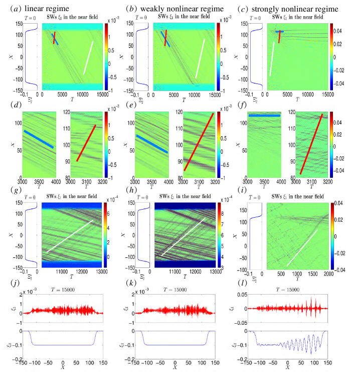
Figure 6: (Colour online) Comparison of spatiotemporal manifestation of SWs in the linear regime ($\vartheta^{\ast}=0,\sigma_{m}=5$E$-4$) [first column], in the weakly nonlinear regime ($\vartheta^{\ast}=1,\sigma_{m}=5$E$-4$) [second column], and in the strongly nonlinear regime ($\vartheta^{\ast}=1,\sigma_{m}=2.5$E$-2$) [third column]. The first row [(a)-(c)] displays the snapshot of the BBF (left panel) and the spatiotemporal evolution of SWs’ profile $\xi_{1}=\Xi_{1}^{*}+\xi_{1}^{*}$ (right panel). The parameters of the BBFs are given in table 1. The second row [(d)-(f)] and the third row [(g)-(i)] display the zoomed-in versions of SWs’ profiles. The red line corresponds to the positive phase velocity of the right-moving short-mode SWs. The white line (blue line) corresponds to the group velocity of right-moving short-mode SWs when SW packets propagate from the trailing (leading) edge towards the leading (trailing) edge. The ranges of color bars in panels (a)-(f) are automatically tuned. To observe the small-amplitude SW packets that propagate from the trailing edge towards the leading edge [white lines], the ranges of color bars in panels (g)-(i) are manually tuned to be smaller. The fourth row [(j)-(l)] displays the snapshots of SWs and IWs at $T=15000$. It can be seen that spatiotemporal manifestation of SWs differs greatly between the linear (or weakly nonlinear) regime and the strongly nonlinear regime. In the strongly nonlinear regime, SW packets are located at the leading edge due to the class 3 triad resonance [see text].

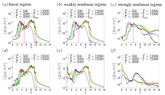
Figure 7: (Colour online) Comparison of wavenumber spectra of SWs and IWs in the linear regime ($\vartheta^{\ast}=0,\sigma_{m}=5$E$-4$) [first column], in the weakly nonlinear regime ($\vartheta^{\ast}=1,\sigma_{m}=5$E$-4$) [second column], and in the strongly nonlinear regime ($\vartheta^{\ast}=1,\sigma_{m}=2.5$E$-2$) [third column]. The first row [(a)-(c)] displays the evolution of the wavenumber spectra of SWs’ $\xi_{1}^{*}$. The bracket $\left\langle\cdot\right\rangle$ is interpreted as an ensemble average over $48$ realizations. The second row [(d)-(f)] displays the evolution of the wavenumber spectra of IWs’ $\xi_{2}^{*}$. All the wavenumber spectra vanish at the initial $T=0$, and these spectra grow as a result of the external pressure $P_{1}$. In the linear and weakly nonlinear regimes, the SW spectrum transits between the intervals $[3,5]$ and $[6.5,9]$ as predicted by the ray-based theory [two green closed curves in figure 3(a)] and thereafter there is a dip at $k_{\text{res}}$ in the SW spectrum. In contrast, in the strongly nonlinear regime, there is a peak growing at $k_{\text{res}}$ in the SW spectrum due to the class 3 triad resonance. Moreover, the IW spectrum grows at $k\approx 0.3$ also due to the class 3 triad resonance.

In this section, we will show that in the strongly-nonlinear regime of the mTWN model, short-mode SWs on the BBF in equation (26) can be located at the leading edge with the resonant wavenumber $k_{\text{res}}\approx 5$ [see figure 5(b) for a description of the resonant wavenumber]. For comparison, we also compute the short-mode SW behavior in the weakly-nonlinear and linear regimes [see appendix A for more discussion of these regimes]. As introduced previously, $\vartheta^{\ast}=0$ corresponds to the linear regime and $\vartheta^{\ast}=1$ corresponds to the nonlinear regime. For $\vartheta^{\ast}=1$, unlike in § 3, we here use the amplitude of the surface pressure $P_{1}$ to control the strength of the nonlinearity. Initially, all wave variables $(\xi_{j}^{\ast},\overline{u}_{j}^{\ast})$ are set to zero. Specifically, we trigger the mTWN system by exerting random pressure $P_{1X}$ only at the initial $T=0$ as follows:

$$P_{1X}=\sigma_{m}\delta\left(T\right)\sum_{k}\sqrt{\left|\tanh\left[s_{L}\left(k-k_{L}\right)\right]-\tanh\left[s_{R}\left(k-k_{R}\right)\right]\right|}\exp\left(\text{i}kX+\text{i}\phi_{k}\right),$$ (33)

where $\sigma_{m}$ controls the strength of the initial perturbation, $\delta\left(T\right)$ is the Kronecker delta function which is 1 when $T=0$ and 0 otherwise, $s_{L}=2.5$, $k_{L}=3$, $s_{R}=1.5$, $k_{R}=4$, and $\phi_{k}$ is a random phase, which is uniformly distributed on $[0,2\pi]$ for each wavenumber $k$. Here, the parameters $s_{L}$, $k_{L}$, $s_{R}$, and $k_{R}$ are empirically chosen such that the initial perturbation waves possess wavenumbers between the two critical wavenumbers $k_{\text{IW}}$ and $k_{\text{res}}$, where $k_{\text{IW}}=0.3$ corresponds to the subsequently-growing peak location of the IW spectrum [figure 7] and $k_{\text{res}}=5$ is the resonant wavenumber of SWs [figure 7]. Next, we focus on the dynamical behavior of the short-mode SWs in both the physical $X$ space and the wavenumber $k$ space for all regimes.

Figure 6 displays the comparison of wave behavior among the linear, weakly nonlinear, and strongly nonlinear regimes. For the linear regime ($\vartheta^{\ast}=0$), it can be seen from figures 6(a)(d)(g) that the SW packets propagate in the direction of decreasing $X$ with a relatively small group velocity [obvious dark stripes parallel to the blue line during the time period about $0\leq T\leq 10000$], and in the direction of increasing $X$ with a relatively large group velocity [faint dark stripes parallel to the white line during the time period about $10000\leq T\leq 14000$]. This zig-zag pattern corresponds to the asymmetric behavior [1a] of the short-mode SWs, as can be predicted by the linear modulation theory. In fact, the obvious and faint dark stripes in figures 6(a)(g) reflect the large amplitude and the small amplitude of the short-mode SWs, respectively. This implies the asymmetric behavior [1c], i.e., that SWs become high at the leading edge and low at the trailing edge.

Moreover, it can be seen from figures 7(a) and (d) that both SW spectra and IW spectra are concentrated around the intervals $[3,5]$ and $[6.5,9]$. Notice that the spectrum of the initial perturbation $P_{1X}$ in equation (33) is concentrated around the interval $[3,4]$, so that, based on the linear modulation theory, the wave spectra should be concentrated around the interval $[6.5,9]$ when SW packets propagate towards the trailing edge [see the two green-level curves in figure 3(a)]. This numerical result implies the asymmetric behavior [1b], i.e., that SWs become short at the leading edge and long at the trailing edge. Note that no IW spectrum grows for $k\leq 2$ [figure 7(d)] and no steep peak forms in the SW spectrum around $k_{\text{res}}$ [figure 7(a)]. Thus, the triad resonance phenomena [2a] and [2b] are not observed in this linear regime. In summary, for the linear regime ($\vartheta^{\ast}=0$), as expected, the asymmetric behavior [1a]-[1c] is observed, while the triad resonance phenomena [2a] and [2b] are not observed. Based on the ray-based theory, the short-mode waves are linearly modulated by the BBF $(\Xi_{j}^{\ast},\overline{U}_{j}^{\ast})$.

In the weakly nonlinear regime ($\vartheta^{\ast}=1,\sigma_{m}=5$E$-4$), we see that the spatiotemporal manifestations of SWs and IWs [figures 6(b)(e)(h)] resemble those of SWs and IWs in the linear regime [figures 6(a)(d)(g)]. In the weakly nonlinear regime, class 3 triad resonance can occur in the near field. It can be seen from figure 7(b) that even the SW spectra resemble those in the linear regime [figure 7(a)]. The only difference arises from the IW spectrum. We see from figure 7(e) that the IW spectrum grows for $k\approx 0.3$ as time increases. This reflects the triad resonance phenomenon [2a], i.e., that the energy is transferred from SWs towards IWs.

For the strongly nonlinear regime ($\vartheta^{\ast}=1,\sigma_{m}=2.5$E$-2$), the behavior of SWs and IWs, in both the $X$ and $k$ spaces, becomes quite different from that in the linear and weakly nonlinear regimes. In the physical $X$ space, surprisingly, one can see from figures 6(c) and (f) that SW packets are trapped at the leading edge of the BBF after some initial time evolution. In the wavenumber $k$ space, both the triad resonance phenomena [2a] and [2b] are observed in figure 7(f) and figure 7(c), respectively. It can be seen from figure 7(f) that IW spectrum grows significantly for $k\approx 0.3$ as time increases, which implies that a significant amount of energy is transferred from SWs towards IWs due to the class 3 triad resonance. It can be seen from figure 7(c) that there is an inverse energy cascade for the spectrum of SWs from larger wavenumbers above $k_{\text{res}}$ towards smaller wavenumbers, and finally a steep peak forms in the spectrum of SWs around $k_{\text{res}}$.

We now propose a possible mechanism, referred to as the modulation-resonance mechanism, underlying this phenomenon, namely, that SWs whose typical wavenumber is the resonant wavenumber $k_{\text{res}}$ are located at the leading edge of the BBF. For convenience of discussing the wave direction, $C_{s}>0$ is assumed for the velocity of the BBF in the rest of the discussion.

(modulation mechanism [3a]) First, after the initial transients, the large-scale BBF separates the left-moving and right-moving short-mode waves. The left-moving radiation quickly leaves the near field, and then only the right-moving waves that propagate in the same direction as the BBF remain trapped in the near field [figure 4].

(modulation mechanism [3a’]) Next, based on the modulation (ray-based) theory, if the right-moving short-mode perturbation waves possess wavenumbers below $k_{\text{res}}$, they are transported towards the leading edge with a relatively large group velocity [long black arrow in figure 3(a) and white line in figure 6(i)]. Also, for right-moving short-mode perturbation waves located in front of the leading edge with wavenumbers larger than $k_{\text{res}}$ [3 rightmost short black arrows in figure 3(a)], they are transported towards the leading edge with a relatively slow group velocity. Thus, SWs are accumulated at the leading edge. During the sloping process at the leading edge, these waves become short in wavelength (wavenumber $k$ becomes $k>k_{\text{res}}$) and high in amplitude. Here, the sloping process means the tendency of short-mode waves to shorten and heighten.

(resonance mechanism [3b]) Finally, since SW packets propagate towards the trailing edge with a relatively small group velocity during the sloping process [3 short black arrows at $X\sim 80$ in figure 3(a) and blue line in figure 6(f)], energy can be accumulated, and meanwhile the amplitude of SWs grows locally at the leading edge as a consequence of the asymmetric behavior [1a]-[1c]. The growing amplitude increases the local nonlinearity significantly and consequently triggers the occurrence of a class 3 triad resonance locally at the leading edge. Then, an inverse energy cascade for the spectrum of SWs emerges, streaming from the larger wavenumbers above $k_{\text{res}}$ towards the smaller wavenumbers, and finally the spectrum of SWs focuses around the $k_{\text{res}}$ [figure 7(c)]. This spectrum evolution indicates that the class 3 triad resonance condition (18) reduces to the resonance condition, $\overline{c}_{g}(k_{\text{res}})=C_{s}$, that is, SW packets propagate at the same velocity as the BBF. Here, $\overline{c}_{g}$ is the modulated group velocity given by $\partial\overline{\omega}_{k}/\partial k$. Therefore, SWs with the resonant wavenumber $k_{\text{res}}$ can be located at the leading edge of the BBF as shown in figure 6(c) and figure 7(c).

In the following §§  4.2 and §§ 4.3, we will examine the robustness of our model results by investigating the behavior of SWs for various underlying BBFs in a parametric study. From the parametric study results, we will supplement an additional resonance mechanism [3b’] to the modulation-resonance mechanism in §§ 4.3.

4.2 Parametric study for parameter regime I

Figure	$X_{\Xi^{\ast}}$	$s_{\Xi^{\ast}}$	$\Xi_{2}^{\ast}(0)$	$\Xi_{1}^{\ast}(0)$	$\overline{U}_{2}^{\ast}(0)$	$\overline{U}_{1}^{\ast}(0)$	$C_{s}$
6(l) [red curve]	120	0.2	-0.1	0.0003	-0.006	0.007	0.0485
8(a) [black curve]	20	0.2	-0.1	0.0003	-0.006	0.007	0.0485
8(a) [blue curve]	70	0.2	-0.1	0.0003	-0.006	0.007	0.0485
8(a) [red curve]	120	0.2	-0.1	0.0003	-0.006	0.007	0.0485
9(e) [black curve]	70	0.022	-0.1	0.0002	-0.0017	0.0044	0.0489
9(e) [blue curve]	70	0.022	-0.2	0.0004	-0.0036	0.0084	0.0502
9(e) [red curve]	70	0.022	-0.3	0.0005	-0.0057	0.0120	0.0513

Table 1: The wavelengths $X_{\Xi^{\ast}}$, slopes $s_{\Xi^{\ast}}$, maximal amplitudes of displacements $\Xi_{j}^{\ast}$, maximal amplitudes of currents $\overline{U}_{j}^{\ast}$, and phase velocities $C_{s}$ of the BBF in equation (26) used for regime I, $(h_{1},h_{2},g,\rho_{1},\rho_{2})=(1,3,1,1,1.003)$. In figure 6, the maximal amplitudes of $(\Xi_{j}^{\ast},\overline{U}_{j}^{\ast})$ and phase velocities are chosen to be close to those of the interfacial solitary wave solutions of the TWN model for $\Xi_{2}^{*}(0)=-0.1$ [see appendix B]. In figures 8 and 9, the maximal amplitudes and phase velocities are chosen to be the same as those of the interfacial solitary wave solutions of the TWN model [see appendix B].

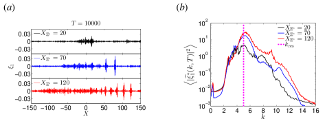
Figure 8: (Colour online) Parameter regime I. (a) Snapshots of SWs $\xi_{1}$ at $T=10000$ for different wavelength $X_{\Xi^{\ast}}$ of the BBF. The parameters of the BBFs are given in table 1. (b) The wavenumber spectra of SWs $\xi_{1}^{*}$. The bracket $\left\langle\cdot\right\rangle$ is interpreted as the time average over $5000\leq T\leq 10000$.

In this section, we investigate how the dynamical behavior of the short-mode SWs is affected by the wavelength $X_{\Xi^{\ast}}$, slope $s_{\Xi^{\ast}}$, and maximal amplitude of $(\Xi_{j}^{\ast},\overline{U}_{j}^{\ast})$ associated with the BBF in equation (26) [table 1] in the strongly nonlinear regime of the parameter regime I, $(h_{1},h_{2},g,\rho_{1},\rho_{2})=(1,3,1,1,1.003)$. After this parametric study, we will further discuss about the modulation-resonance mechanism in next §§ 4.3. The initial driving force $P_{1X}$ adopted here is exactly the same as the force corresponding to the strongly nonlinear regime in the previous section [equation (33)]. First, we study the effects of BBF’s wavelength $X_{\Xi^{\ast}}$ on the dynamical behavior of short-mode SWs. It can be seen from figure 8(a) that the longer the wavelength of the BBF, the larger the number of SW packets that can be trapped at the leading edge in $X$ space. From figure 8(b), it can be seen that the wavenumber spectra of SWs focus around the resonant wavenumber $k_{\text{res}}$. It can be further observed that the longer the wavelength of the BBF, the higher the peak of the SWs’ spectrum around the resonant $k_{\text{res}}$.

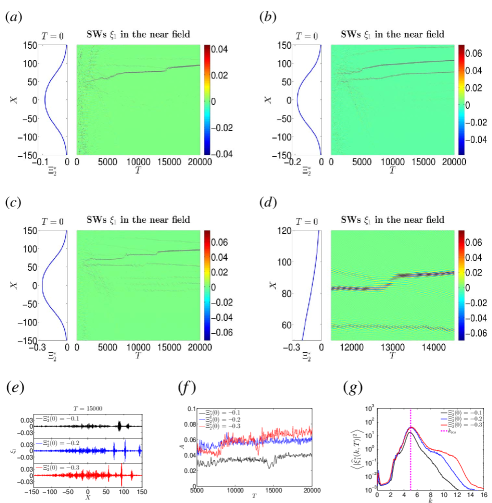
Figure 9: (Colour online) Parameter regime I. The snapshot of the BBF (left panel) and the corresponding spatiotemporal evolution of SWs’ profile $\xi_{1}$ (right panel) for the different maximal amplitude of the BBF being (a) $\Xi_{2}^{\ast}(0)=-0.1$, (b) $\Xi_{2}^{\ast}(0)=-0.2$, and (c) $\Xi_{2}^{\ast}(0)=-0.3$. The parameters of the BBFs are given in table 1. (d) Zoomed-in version of (c) for $11500\leq T\leq 14500$ for the maximal amplitude of the BBF being $\Xi_{2}^{\ast}(0)=-0.3$. (e) Snapshots of SWs’ profile $\xi_{1}$ at $T=15000$ for different maximal amplitudes of the BBFs. (f) The temporal evolution of the maximal amplitude, $A$, of the SWs. (g) The wavenumber spectra of SWs $\xi_{1}^{*}$. The bracket $\left\langle\cdot\right\rangle$ is interpreted as the time average over $5000\leq T\leq 20000$. The resonant wavenumber $k_{\text{res}}=5.0$ as depicted by the magenta line.

Next, we study the effects of BBF’s slope $s_{\Xi^{\ast}}$ on the dynamical behavior of short-mode SWs. Note that figures 6–8 correspond to the relatively large slope ($s_{\Xi^{\ast}}=0.2$), whereas figure 9 corresponds to the relatively small slope ($s_{\Xi^{\ast}}=0.022$) of the BBF. In $k$ space, wavenumber spectra of SWs behave similarly, that is, wave spectra focus around the resonant $k_{\text{res}}$. In $X$ space, however, the spatiotemporal manifestations of SWs differ between large and small slopes of BBF. For a large slope [figures 6 and 8], SWs are generated in several size-ordered packets [about 6 packets in figure 6(l)] with the larger amplitudes appearing at the leading edge of the BBF, which then slowly decay to smaller amplitudes at the trailing edge. However, for the small slope, SWs are generated in only one to three dominant wave packets at the leading edge [figure 9]. For the largest dominant wave packet, both of its maximal amplitude and group velocity increase after the interaction with other smaller-amplitude wave packets. For example, it can be seen from figures 9(d) and (f) that after the dominant wave packet interacts with a smaller-amplitude wave packet at $T=13000$, its amplitude becomes slightly larger [figure 9(f)] and its group velocity becomes slightly faster [figure 9(d)]. At the same time, the small-amplitude wave packet becomes even smaller after the interaction [figure 9(d)]. During this process, energy may be transferred from the smaller-amplitude wave packet to the larger-amplitude one.

Last, we study the effects of BBF’s maximal amplitude, $(\Xi_{j}^{\ast}(0),\overline{U}_{j}^{\ast}(0))$, on the dynamical behavior of short-mode SWs. It can be seen from figure 9(f) that, for larger maximal-amplitude of the BBF, the dominant SW packet with a larger amplitude can be generated at the leading edge. Also, it can be seen from figure 9(g) that, for larger maximal-amplitude of the BBF, the peak of the SWs’ spectrum is higher in amplitude around the resonant $k_{\text{res}}$.

4.3 Parametric study for parameter regime II

To confirm the modulation-resonance mechanism, we choose a different parameter regime II, $(h_{1},h_{2},g,\rho_{1},\rho_{2})=(1,5,1,0.856,0.996)$, for studying the dynamical behavior of the short-mode SWs. This parameter regime was studied in Ref. (Kodaira et al., 2016). The initial driving force $P_{1X}$ adopted here is in the form of equation (33) with $s_{L}=2.5$, $k_{L}=0.3$, $s_{R}=1.5$, $k_{R}=1$, and $\sigma_{m}=2.5$E$-2$. Again, we investigate the effects of the wavelength $X_{\Xi^{\ast}}$, slope $s_{\Xi^{\ast}}$, and maximal amplitude of $(\Xi_{j}^{\ast},\overline{U}_{j}^{\ast})$ associated with the BBF in equation (26) [table 2] on the short-mode SWs in the strongly nonlinear regime.

First, for a relatively small-wavelength BBF ($X_{\Xi^{\ast}}=100$), SW packets at the leading edge have almost the same amplitudes as those at the trailing edge [black curve in figure 10(a)]. However, for a relatively large-wavelength BBF ($X_{\Xi^{\ast}}=150$ and $200$), SWs packets at the leading edge have larger amplitudes than those at the trailing edge [figure 10(a), blue curve and red curve]. Thus, SW packets can be observed at the leading edge when the wavelength of the BBF is sufficiently large. In $k$ space, the spectra of SWs focus around the resonant wavenumber $k_{\text{res}}$ [magenta line in figure 10(b)], where the modulated dispersion relation (27) [$(\Xi_{1}^{\ast},\Xi_{2}^{\ast},\overline{U}_{1}^{\ast},\overline{U}_{2}^{\ast})=(0.025,-0.24,0.08,-0.02)$] is applied in the resonance condition (19). For comparison, we also plot the the resonant wavenumber $k_{\text{res}}$ [green line] where the pure linear dispersion relation $\mu_{k}$ [equation (15)] is used in the resonance condition (19). One can see that the peak locations of the SWs’ spectra are in good agreement with the resonant $k_{\text{res}}$ using the modulated dispersion relation (27) as shown in figure 10(b). Thus, it is the modulated dispersive waves for short-modes, instead of the pure linear dispersive waves, that interact with the long-mode wave through a class 3 triad resonance. [For parameter regime I, we have not plotted the resonant $k_{\text{res}}$ using the pure linear dispersion relation for comparison since both resonant wavenumbers $k_{\text{res}}$ are very close to each other. That is, the resonant $k_{\text{res}}=4.9$ using the pure linear dispersion relation whereas the resonant $k_{\text{res}}=5.0$ using the modulated dispersion relation.] Note that it has been earlier reported by Kodaira et al. (2016) that the modulated dispersion relation should be used when there is an underlying internal wave.

Figure	$X_{\Xi^{\ast}}$	$s_{\Xi^{\ast}}$	$\Xi_{2}^{\ast}(0)$	$\Xi_{1}^{\ast}(0)$	$\overline{U}_{2}^{\ast}(0)$	$\overline{U}_{1}^{\ast}(0)$	$C_{s}$
10(a) [black curve]	100	0.2	-0.24	0.025	-0.02	0.08	0.38
10(a) [blue curve]	150	0.2	-0.24	0.025	-0.02	0.08	0.38
10(a) [red curve]	200	0.2	-0.24	0.025	-0.02	0.08	0.38
11(d) [black curve]	90	0.0167	-0.24	0.025	-0.02	0.08	0.38
11(d) [blue curve]	90	0.0167	-0.77	0.060	-0.08	0.19	0.43
11(d) [red curve]	90	0.0167	-1.21	0.084	-0.14	0.25	0.45

Table 2: The wavelengths $X_{\Xi^{\ast}}$, slopes $s_{\Xi^{\ast}}$, maximal amplitudes $(\Xi_{j}^{\ast}(0),\overline{U}_{j}^{\ast}(0))$, and velocities $C_{s}$ of the BBF in equation (26) used for regime II $(h_{1},h_{2},g,\rho_{1},\rho_{2})=(1,5,1,0.856,0.996)$ [see this parameter regime in (Kodaira et al., 2016)]. In figures 10 and 11, the maximal amplitudes and phase velocities are chosen to be the same as those of the interfacial solitary wave solutions of the TWN model [see appendix B].

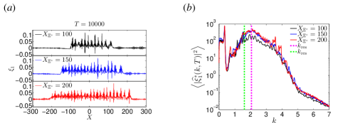
Figure 10: (Colour online) Parameter regime II. (a) Snapshots of SWs $\xi_{1}$ at $T=10000$ for different wavelength $X_{\Xi^{\ast}}$ of the BBF. The parameters of the BBFs are given in table 2. (b) The wavenumber spectra of SWs $\xi_{1}^{*}$. The bracket $\left\langle\cdot\right\rangle$ is interpreted as the time average over $5000\leq T\leq 10000$. The resonant wavenumber $k_{\text{res}}$ depicted by the green line is $1.6$, where the pure linear dispersion relation $\mu_{k}$ [equation (15)] is used in the resonance condition (19). The resonant wavenumber $k_{\text{res}}$ depicted by the magenta line is $2.1$, where the modulated dispersion relation (27) with $(\Xi_{1}^{\ast},\Xi_{2}^{\ast},\overline{U}_{1}^{\ast},\overline{U}_{2}^{\ast})=(0.025,-0.24,0.08,-0.02)$ is used in the resonance condition (19).

Next, by comparing the results in figures 10 and 11, we can see that SWs are generated in several wave packets for the large-slope BBF ($s_{\Xi^{\ast}}=0.2$) [figure 10], whereas SWs are generated in only one dominant wave packet at the front followed by a small-amplitude dispersive tail for the small-slope BBF ($s_{\Xi^{\ast}}=0.0167$) [figure 11]. Again, the dominant wave packet becomes higher in amplitude and faster in group velocity after the interaction with many small-amplitude modulated dispersive waves [figures 11(a)(b)(c)(e)]. One can observe that once the amplitude of the dominant wave packet is large enough, its speed can exceed the speed of the BBF and then move even beyond the leading edge.

Figure 11: (Colour online) Parameter regime II. The snapshot of the BBF (left panel) and the spatiotemporal evolution of SWs’ profile $\xi_{1}$ (right panel) with the maximal amplitude of the BBF being (a) $\Xi_{2}^{\ast}(0)=-0.24$, (b) $\Xi_{2}^{\ast}(0)=-0.77$, and (c) $\Xi_{2}^{\ast}(0)=-1.21$. The parameters of the BBFs are given in table 2. (d) Snapshots of SWs’ profile $\xi_{1}$ at $T=15000$ for different maximal amplitudes of the BBF. (e) The temporal evolution of the maximal amplitude, $A$, of the SWs. (f) The wavenumber spectra of SWs’ $\xi_{1}^{*}$. The bracket $\left\langle\cdot\right\rangle$ is interpreted as the time average over $5000\leq T\leq 15000$. The resonant wavenumber $k_{\text{res}}=2.1$ as depicted by the magenta line.

Finally, for the larger-amplitude of the BBF, the dominant SW packet can grow higher in amplitude at the leading edge [figure 11(e)]. In figure 11(f), we still plot the resonant wavenumber $k_{\text{res}}=2.1$ for reference. One can see that for the larger-amplitude BBF, the peak of the SW spectrum becomes higher in amplitude and also the resonant wavenumber becomes slightly larger.

In summary, the effects of BBF’s wavelength, slope, and amplitude on the dynamical behavior of short-mode SWs can be summarized as follows:

[4a] SWs can be trapped at the leading edge only when the wavelength of the BBF is sufficiently long [figure 8 or figure 10].

[4b] Fewer numbers of SW packets are generated at the leading edge when the slope of the BBF is smaller [comparing figures 8 and 9 or comparing figures 10 and 11].

[4c] SW packets are larger in amplitude at the leading edge when the amplitude of the BBF is larger [figure 9 or figure 11].

Based on the above parametric study of the BBF on the dynamical behavior of short-mode SWs, an additional statement can be supplemented in the description of the modulation-resonance mechanism as discussed in §§ 4.1, namely,

(resonance mechanism [3b’]) If the slope of the BBF is relatively small, only one or very few dominant ($X$-space localized large-amplitude) wave packets can be generated at the leading edge. These localized wave packets become high in amplitude and large in group velocity after the interaction with other smaller-amplitude wave packets [figure 9] or with background perturbation waves [figure 11].

Our understanding of this numerical result is provided as follows: Modulation mechanism [3a’] cannot contribute to the growth of the dominant SW packet’s amplitude and group velocity since, in the linear modulation theory, the amplitude of a SW packet grows only when it propagates towards the trailing edge [figure 3]. Also, dispersive effect cannot contribute to this growth since dispersion can only reduce the maximal amplitude of the dominant wave packet [figures 3 and 4(c)]. Thus, only nonlinear effects can contribute to the growing amplitude of the dominant SW packet. Due to the modulation mechanism [3a], left-moving and right-moving waves are initially separated and only right-moving waves remain at the leading edge after long-time evolution. Therefore, only the nonlinear class 3 triad resonance can contribute to the growing amplitude of these co-propagating SWs. This possibly results from the inverse energy cascade flowing from the spectrum of surrounding perturbation waves with larger wavenumbers above $k_{\text{res}}$ towards the dominant SW packets with characteristic wavenumber $k_{\text{res}}$. In summary, when the slope of the BBF is small, one SW packet or very few SW packets, localized in both $X$ and $k$ spaces, can be generated at the leading edge of the underlying BBF.

5 Conclusions and discussion

We have investigated the coupling between SWs and IWs on a BBF in our modified two-layer weakly-nonlinear (mTWN) model. The mTWN model  possesses a class 3 triad resonance between two short-mode waves and one long-mode wave. In §§ 3.1, we have reviewed four asymmetric behavior types of short-mode waves ([1a]-[1d]), as can be seen in the mTWN model and predicted by the linear modulation (ray-based) theory. In §§ 3.2, using the mTWN model, we have reproduced the class 3 triad resonance phenomena [2a] and [2b], as mentioned by Tanaka & Wakayama (2015).

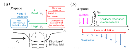
Figure 12: (Colour online) Sketch of the modulation-resonance mechanism [see text] (a) in the $X$ space and (b) in the $k$ space.

In § 4, we have addressed two important features of SW dynamics driven by an underlying BBF, that is, a finite number of $X$-space-localized SW packets with $k$-space-localized resonant wavenumber can be generated at the leading edge of the BBF [figures 6 and 7]. From our parametric study, we further observe that, for a sufficiently slowly-varying, long-wavelength, large-amplitude BBF, one or very few dominant SW packets with growing amplitude and group velocity can be generated at the leading edge [figures 9 and 11].

Subsequently, we have proposed a possible modulation-resonance mechanism for understanding these surface phenomena in our numerical results. The mechanism is sketched in figure 12. First, based on the modulation mechanisms [3a] and [3a’], SW packets propagate with a relatively large group velocity towards the leading edge of the BBF and a sink of SW packets is thereafter formed at the leading edge. Next, based on the resonance mechanisms [3b] and [3b’], the spectrum of SWs is concentrated near the resonant wavenumber, and simultaneously these resonant SWs become high in amplitude at the leading edge. This modulation-resonance mechanism may be responsible for the experimental observations of (i) the surface roughness at the leading edge in the $X$ space and (ii) resonant excitations of SWs in the $k$ space (Osborne & Burch, 1980; Kropfli et al., 1999).

As discussed in the introduction, several previous works used asymptotic analysis to obtain effective reduced models for addressing the surface signature of an IW (Kawahara et al., 1975; Hashizume, 1980; Funakoshi & Oikawa, 1983; Donato et al., 1999; Parau & Dias, 2001; Bakhanov & Ostrovsky, 2002; Barros & Gavrilyuk, 2007; Hwung et al., 2009; Craig et al., 2012). These reduced models mostly focus on either the dynamics of short-mode waves around the resonant $k_{\text{res}}$ at sufficiently long times or the linear modulations and the traveling wave solutions for short-mode surface waves. A particularly detailed prior discussion of surface signature phenomena was presented in (Craig et al., 2012) using a coupled Korteweg–de Vries (KdV) and linear Schrödinger model (we compare this model with ours in appendix D). However, an intuitive understanding of the surface signature phenomena was still lacking, especially for the asymmetric behavior of SWs at the leading and trailing edges. Our work in the present paper is an attempt to provide some of this understanding.

We now draw several conclusions regarding our work. First, we point out the reach of our modeling. The mTWN model consists of Boussinesq-type equations describing the dynamics of long-wavelength ($10$-$100$ m) short-mode barotropic SWs with an underlying even longer-wavelength ($10$-$1000$ km) baroclinic flow in the shallow-water configuration [see the dimensionless form of the mTWN model in appendix A]. The dispersion relation of the mTWN model differs from that of the Euler system. The advantage of the mTWN model is in being computationally cheap, which allows us to study the long-time dynamical behavior of these short-mode SWs. However, the long-wave approximation (10) for short-mode SWs is not appropriate for a quantitative description of short-wavelength (0.1-1 m) SWs in the presence of an underlying 1 km internal wave studied in many field observations (Gargett & Hughes, 1972; Osborne & Burch, 1980; Kropfli et al., 1999). Note that short-mode SWs, corresponding to the dispersion relation $\omega_{k}$ [equation (17)] in the TWN model or the modulated dispersion relation $\overline{\omega}$ [equation (27)] in the mTWN model, only means the wavelength of the barotropic SWs is relatively short with respect to the baroclinic flow, and it does not mean the wavelength of SWs itself is short. In addition, we point out that our goal in this paper is to only qualitatively, instead of quantitatively, capture these 0.1-1 m surface signatures of an internal wave. In future work addressing the quantitative surface signature, the long-wave approximation (10) should be removed to investigate the dynamical behavior of short-wavelength (0.1-1 m) SWs with an underlying $\sim 1$ km IW in the two-layer Euler system.

Second, we address how our results are qualitatively consistent with surface phenomena (i) and (ii) in field observations. In particular, we point out the following three aspects: (1) Asymmetric behavior [1a]-[1d] can also be found in the two-layer Euler system (Lewis et al., 1974; Bakhanov & Ostrovsky, 2002; Kodaira et al., 2016), and is predicted by the linear modulation (ray-based) theory (Lewis et al., 1974; Kodaira et al., 2016). In our mTWN model, similar asymmetric behavior of SWs can be found and also predicted by the linear modulation theory [§§ 3.1]. (2) The nonlinear class 3 triad resonance phenomena [2a] and [2b] were observed in the two-layer Euler system by Tanaka & Wakayama (2015). In our mTWN model, such nonlinear triad resonance phenomena can also be reproduced [§§ 3.2]. (3) Our model predicts that, in the strongly nonlinear regime, one spatially-localized large-amplitude SW packet with wavelength $10$-$100$ m can be generated at the leading edge of an underlying slowly-varying baroclinic flow with wavelength $10$-$1000$ km. Qualitatively, our result is consistent with the surface phenomena in many field observations from which a narrow band of $0.1$-$1$ m SWs is located at the leading edge of an underlying $1$ km internal solitary wave (Gargett & Hughes, 1972; Osborne & Burch, 1980). These three aspects allow us to claim that our numerical results are qualitatively consistent with IW surface signature reported from many field observations. From the qualitatively-consistent results, we have gained intuition regarding the sizes of two important parameters $\gamma$ (wavelength ratio of long-mode and short-mode waves) and $\vartheta$ (nonlinearity) in our mTWN model as discussed in detail in appendix A. It may be helpful to rigorously study the asymptotics of these SWs in the two-layer Euler system.

Third, our model results predict that, in the weakly nonlinear regime, short-mode SWs that propagate in the same direction as the underlying baroclinic flow can be trapped in the near field, propagating back and forth, and eventually almost uniformly distribute themselves with small amplitudes in the near field due to the wave dispersion. This might be related to the phenomenon that small-amplitude SWs accompany with internal tides of the scale around $100$ km (Johnston et al., 2003). In the strongly nonlinear regime, our model results predict that very few SW packets can be generated locally at the leading edge of the underlying BBF and they become high in amplitude and large in group velocity after interacting with the surrounding waves. The behavior of these $X$-space-localized, large-amplitude SW packets might be related to rogue wave phenomena (Müller et al., 2005; Dysthe et al., 2008).

Finally, also most importantly, we combine the modulation mechanism and resonance mechanism to understand our numerical results concerning SWs localized in both $X$ and $k$ spaces obtained from the mTWN model. We hypothesize that our combined modulation-resonance mechanism may be extended to the two-layer Euler system in both shallow- and deep-water configurations and other density-stratified systems that admit a class 3 triad resonance [see more discussion in appendix A]. As long as the baroclinic flow has a slight non-uniformity on a sufficiently large scale, and the perturbation waves are strong enough, a localized wave packet with the typical resonant wavenumber may be generated at the leading edge of the baroclinic flow. Further investigation is needed to examine this hypothesis. We relegate this investigation to future work.

6 Acknowledgements

This work is supported by NYU Abu Dhabi Institute G1301(D.C., D.Z.), NSFC Grant No. 11671259, 11722107, and 91630208, NSFC Grant No. 31571071 (D.C.), and SJTU-UM Collaborative Research Program (D.C., D.Z.). We thank Yuri V. Lvov and Wooyoung Choi for helpful comments. We dedicate this paper to our late coauthor and mentor D.C. who conceived and designed this project.

Appendix A Dimensionless forms and some discussions of the TWN and mTWN models

In this appendix, we will provide dimensionless forms of the TWN and mTWN models and then discuss the asymptotics and typical scaling of the mTWN model. First, we provide the dimensionless form of the TWN model. Based on the two approximations $a/h_{1}=\alpha\ll 1$ [equation (9)] and $h_{1}^{2}/l^{2}=\beta\ll 1$ [equation (10)], we non-dimensionalize all the variables as follows:

$$x =lx^{\prime},\text{ \ \ }t=\left(l/U_{0}\right)t^{\prime},$$

$$\overline{u}_{j} =\alpha U_{0}\overline{u}_{j}^{\prime},\text{ \ }\xi_{j}=a\xi_{j}^{\prime},\text{ \ }P_{1}=\alpha\rho_{1}U_{0}^{2}P_{1}^{\prime},$$

where $U_{0}$ is the characteristic speed chosen as $U_{0}=\sqrt{gh_{1}}$, and all the variables adorned with primes are $O(1)$ in $\alpha$ and $\beta$. Using asymptotic analysis similar to that for the KdV equation (Whitham, 1974) and retaining the terms in the first power of $\alpha$ and $\beta$, we obtain the TWN model (11)-(14) in the dimensionless form,

$$\eta_{1t^{\prime}}^{\prime}+(\eta_{1}^{\prime}\overline{u}_{1}^{\prime})_{x^{\prime}}=0,\text{ \ \ }\eta_{1}^{\prime}=h_{1}^{\prime}+\alpha\xi_{1}^{\prime}-\alpha\xi_{2}^{\prime},$$ (34)

$$\eta_{2t^{\prime}}^{\prime}+(\eta_{2}^{\prime}\overline{u}_{2}^{\prime})_{x^{\prime}}=0,\text{ \ \ }\eta_{2}^{\prime}=h_{2}^{\prime}+\alpha\xi_{2}^{\prime},$$ (35)

$$\overline{u}_{1t^{\prime}}^{\prime}+\alpha\overline{u}_{1}^{\prime}\overline{u}_{1x^{\prime}}^{\prime}+g^{\prime}\xi_{1x}^{\prime}-\frac{1}{3}\beta h_{1}^{\prime 2}\overline{u}_{1x^{\prime}x^{\prime}t^{\prime}}^{\prime}+\frac{1}{2}\beta h_{1}^{\prime}\xi_{2x^{\prime}t^{\prime}t^{\prime}}^{\prime}+P_{1x^{\prime}}^{\prime}=O\left(\alpha^{2},\beta^{2}\right),$$ (36)

$$\overline{u}_{2t^{\prime}}^{\prime}+\alpha\overline{u}_{2}^{\prime}\overline{u}_{2x^{\prime}}^{\prime}+g^{\prime}\xi_{2x^{\prime}}^{\prime}+\rho_{r}g^{\prime}\left(\xi_{1}^{\prime}-\xi_{2}^{\prime}\right)_{x^{\prime}}$$ (37)

$$-\frac{1}{2}\beta\rho_{r}h_{1}^{\prime 2}\overline{u}_{1x^{\prime}x^{\prime}t^{\prime}}^{\prime}+\beta\rho_{r}h_{1}^{\prime}\xi_{2x^{\prime}t^{\prime}t^{\prime}}^{\prime}-\frac{1}{3}\beta h_{2}^{\prime 2}\overline{u}_{2x^{\prime}x^{\prime}t^{\prime}}^{\prime}+P_{1x^{\prime}}^{\prime}\rho_{1}/\rho_{2}=O\left(\alpha^{2},\beta^{2}\right),$$

where

$$h_{1}^{\prime}=1,\text{ \ }h_{2}^{\prime}=h_{2}/h_{1},\text{ \ }g^{\prime}=1.$$

Next, we provide the derivation of our mTWN model. We begin with the dimensional TWN model describing the coupling of long waves for two layers of fluids with unequal densities. The variables $(\xi_{j},\overline{u}_{j})$ in the dimensional TWN model are represented as a sum of the BBF and perturbations of barotropic short-mode waves,

$$(\xi_{j},\overline{u}_{j})=(\Xi_{j}^{\ast},\overline{U}_{j}^{\ast})+(\xi_{j}^{\ast},\overline{u}_{j}^{\ast}),$$ (38)

where $(\Xi_{j}^{\ast},\overline{U}_{j}^{\ast})$ denotes the BBF and $(\xi_{j}^{\ast},\overline{u}_{j}^{\ast})$ denotes the perturbation waves. Based on the assumption (21), there is a scale separation of wavelengths between the BBF $(\Xi_{j}^{\ast},\overline{U}_{j}^{\ast})$ and perturbation waves $(\xi_{j}^{\ast},\overline{u}_{j}^{\ast})$. Since we are interested in the dynamics of short-mode perturbation waves, we choose the characteristic time and space scalings for these short-mode waves such that the chosen scalings are self-consistent with our numerical results for the TWN model. We non-dimensionalize all variables $(\Xi_{j}^{\ast},\overline{U}_{j}^{\ast})$ and $(\xi_{j}^{\ast},\overline{u}_{j}^{\ast})$ as follows:

$$x =lx^{\prime},\text{ \ \ }t=\left(l/U_{0}\right)t^{\prime},\text{ \ }P_{1}=\rho_{1}u_{0}U_{0}P_{1}^{\prime},$$

$$\overline{U}_{j}^{\ast} =U_{0}\overline{U}_{j}^{\prime},\text{ \ }\overline{u}_{j}^{\ast}=u_{0}\overline{u}_{j}^{\prime},\text{ \ }\Xi_{j}^{\ast}=A\Xi_{j}^{\prime},\text{ \ }\xi_{j}^{\ast}=a\xi_{j}^{\prime},$$ (39)

where $l$ is the characteristic wavelength of the short-mode waves, $U_{0}$ and $u_{0}$ are the characteristic speeds of the BBF and the short-mode waves, respectively, and $A$ and $a$ are the characteristic amplitudes of the BBF and the short-mode waves, respectively. We further apply the following assumptions:

[1] The dimensionless BBF, $(\Xi_{j}^{\prime},\overline{U}_{j}^{\prime})$, is a right-moving traveling wave with the phase velocity $C_{s}$ satisfying,

$$\Xi_{j}^{\prime}=\Xi_{j}^{\prime}\left(X^{\prime}\right),\text{ \ }\overline{U}_{j}^{\prime}=\overline{U}_{j}^{\prime}\left(X^{\prime}\right)\text{ \ with }X^{\prime}=K\left(x-C_{s}t\right),\text{ }K=2\pi/L,\text{ \ }$$ (40)

where $L$ is the characteristic wavelength of the BBF. Here, the derivatives of the dimensionless BBF are of $O\left(1\right)$, that is, $d\Xi_{j}^{\prime}/dX^{\prime}=O\left(1\right)$ and $d\overline{U}_{j}^{\prime}/dX^{\prime}=O\left(1\right)$.

[2] The characteristic wavelength of the short-mode waves, $l$, is much shorter than the characteristic wavelength of the BBF, $L$, (Hwung et al., 2009)

$$2\pi l/L=\gamma\ll 1.$$ (41)

[3] For the BBF, the characteristic amplitude $A$ and the characteristic speed $U_{0}$ satisfy,

$$A=h_{1},\text{ \ \ }U_{0}=\sqrt{gh_{1}}.$$ (42)

[4] For the short-mode waves, the characteristic amplitude $a$ and the characteristic speed $u_{0}$ satisfy

$$a=\vartheta h_{1},\text{ \ \ }u_{0}=\vartheta\sqrt{gh_{1}},\text{ \ }$$ (43)

where the parameter $\vartheta$ controls the relative scaling between the short-mode waves and the BBF.

[5] The characteristic wavelength of the short-mode wave, $l$, satisfies

$$l=h_{1},$$ (44)

which is self-consistent with our numerical results [figures 2-11]. Here, note that from the numerical results, the characteristic wavelength of the resonant short-mode waves is $l\sim 2\pi/k_{\text{res}}=1.25$, which is on the same order of $h_{1}=1$ [see figure 2(b) for example].

All variables adorned with primes are $O(1)$ in $\gamma$. Substituting the sum (38), the non-dimensionalization (39), and the assumptions (40)-(44) into our TWN model, we obtain the model in the following dimensionless form:

$$\eta_{1t^{\prime}}^{\prime}+\left[h_{1}^{\prime}\overline{u}_{1}^{\prime}+\left(\Xi_{1}^{\prime}-\Xi_{2}^{\prime}\right)\overline{u}_{1}^{\prime}+\overline{U}_{1}^{\prime}(\xi_{1}^{\prime}-\xi_{2}^{\prime})+\vartheta(\xi_{1}^{\prime}-\xi_{2}^{\prime})\overline{u}_{1}^{\prime}\right]_{x^{\prime}}$$ (45)

$$-\frac{\gamma}{\vartheta}\frac{C_{s}}{U_{0}}H_{1X^{\prime}}^{\prime}+\frac{\gamma}{\vartheta}h_{1}^{\prime}\overline{U}_{1X^{\prime}}^{\prime}+\frac{\gamma}{\vartheta}\left(\left(\Xi_{1}^{\prime}-\Xi_{2}^{\prime}\right)\overline{U}_{1}^{\prime}\right)_{X^{\prime}}=0,$$

$$\eta_{2t^{\prime}}^{\prime}+\left[h_{2}^{\prime}\overline{u}_{2}^{\prime}+\Xi_{2}^{\prime}\overline{u}_{2}^{\prime}+\overline{U}_{2}^{\prime}\xi_{2}^{\prime}+\vartheta\xi_{2}^{\prime}\overline{u}_{2}^{\prime}\right]_{x^{\prime}}$$ (46)

$$-\frac{\gamma}{\vartheta}\frac{C_{s}}{U_{0}}H_{2X^{\prime}}^{\prime}+\frac{\gamma}{\vartheta}h_{2}^{\prime}\overline{U}_{2X^{\prime}}^{\prime}+\frac{\gamma}{\vartheta}\left(\overline{U}_{2}^{\prime}\Xi_{2}^{\prime}\right)_{X^{\prime}}=0,$$

$$\overline{u}_{1t^{\prime}}^{\prime}+\left(\overline{U}_{1}^{\prime}\overline{u}_{1}^{\prime}+\frac{1}{2}\vartheta\overline{u}_{1}^{\prime 2}+g^{\prime}\xi_{1}^{\prime}\right)_{x^{\prime}}-\frac{1}{3}h_{1}^{\prime 2}\overline{u}_{1x^{\prime}x^{\prime}t^{\prime}}^{\prime}+\frac{1}{2}h_{1}^{\prime}\xi_{2x^{\prime}t^{\prime}t^{\prime}}^{\prime}+P_{1x^{\prime}}^{\prime}$$ (47)

$$-\frac{\gamma}{\vartheta}\frac{C_{s}}{U_{0}}\overline{U}_{1X^{\prime}}^{\prime}+\frac{\gamma}{\vartheta}\overline{U}_{1}^{\prime}\overline{U}_{1X^{\prime}}^{\prime}+\frac{\gamma}{\vartheta}g^{\prime}\Xi_{1X^{\prime}}^{\prime}+\frac{1}{3}\frac{\gamma^{3}}{\vartheta}\frac{C_{s}}{U_{0}}h_{1}^{\prime 2}\overline{U}_{1X^{\prime}X^{\prime}X^{\prime}}^{\prime}+\frac{1}{2}\frac{\gamma^{3}}{\vartheta}\frac{C_{s}^{2}}{U_{0}^{2}}h_{1}^{\prime}\Xi_{2X^{\prime}X^{\prime}X^{\prime}}^{\prime}=0,$$

$$\overline{u}_{2t^{\prime}}^{\prime}+\left(\overline{U}_{2}^{\prime}\overline{u}_{2}^{\prime}+\frac{1}{2}\vartheta\overline{u}_{2}^{\prime 2}+g^{\prime}\xi_{2}^{\prime}+\rho_{r}g^{\prime}\eta_{1}^{\prime}\right)_{x^{\prime}}$$ (48)

$$-\frac{1}{2}\rho_{r}h_{1}^{\prime 2}\overline{u}_{1x^{\prime}x^{\prime}t^{\prime}}^{\prime}+\rho_{r}h_{1}^{\prime}\xi_{2x^{\prime}t^{\prime}t^{\prime}}^{\prime}-\frac{1}{3}h_{2}^{\prime 2}\overline{u}_{2x^{\prime}x^{\prime}t^{\prime}}^{\prime}+P_{1x^{\prime}}^{\prime}\rho_{1}/\rho_{2}$$

$$-\frac{\gamma}{\vartheta}\frac{C_{s}}{U_{0}}\overline{U}_{2X^{\prime}}^{\prime}+\frac{\gamma}{\vartheta}\overline{U}_{2}^{\prime}\overline{U}_{2X^{\prime}}^{\prime}+\frac{\gamma}{\vartheta}g^{\prime}\Xi_{2X^{\prime}}^{\prime}+\frac{\gamma}{\vartheta}\rho_{r}g^{\prime}H_{1X^{\prime}}^{\prime}$$

$$+\frac{1}{2}\frac{\gamma^{3}}{\vartheta}\frac{C_{s}}{U_{0}}\rho_{r}h_{1}^{\prime 2}\overline{U}_{1X^{\prime}X^{\prime}X^{\prime}}^{\prime}+\frac{\gamma^{3}}{\vartheta}\frac{C_{s}^{2}}{U_{0}^{2}}\rho_{r}h_{1}^{\prime}\Xi_{2X^{\prime}X^{\prime}X^{\prime}}^{\prime}+\frac{1}{3}\frac{\gamma^{3}}{\vartheta}\frac{C_{s}}{U_{0}}h_{2}^{\prime 2}\overline{u}_{2X^{\prime}X^{\prime}X^{\prime}}^{\prime}=0,$$

where

$$h_{1}^{\prime}=1,\text{ \ }h_{2}^{\prime}=h_{2}/h_{1},\text{ \ }g^{\prime}=1,$$

$$H_{1}^{\prime}=h_{1}^{\prime}+\Xi_{1}^{\prime}-\Xi_{2}^{\prime},\text{ \ \ }H_{2}^{\prime}=h_{2}^{\prime}+\Xi_{2}^{\prime},\text{ \ }$$

$$\eta_{1}^{\prime}=h_{1}^{\prime}+\xi_{1}^{\prime}-\xi_{2}^{\prime},\text{ \ \ }\eta_{2}^{\prime}=h_{2}^{\prime}+\xi_{2}^{\prime}.$$

In the limit of

$$\gamma\rightarrow 0,$$ (49)

we obtain the dimensionless mTWN model. Casting the mTWN system in the conservation form in the right-moving frame with the velocity $C_{s}$, we can obtain our mTWN model, in dimensional form, in the equations of (22)-(25). Since the interfacial solitary wave solutions in the TWN model [see figure 13 in the following appendix B] are not long enough in wavelength to satisfy the assumption (49), we instead use a slowly-varying, long-wavelength BBF in the mTWN model. This is the reason why we use the mTWN model instead of the TWN model in our investigation.

We now discuss the asymptotics for the mTWN model.

[1] If $\vartheta=0$ (or equivalently $\vartheta\rightarrow 0$ and $\gamma/\vartheta\rightarrow 0$), the model corresponds to the linear regime [1st column of figure 6];

[2] if $\vartheta\ll 1$, the model corresponds to the weakly nonlinear regime [2nd column of figure 6];

[3] if $\vartheta=O\left(1\right)$, the model corresponds to the strongly nonlinear regime [3rd column of figure 6].

When $\vartheta=0$, short-mode waves satisfy the modulated dispersion relation (27) instead of the pure linear dispersion relation (15). For short-time dynamics, we can see the phase velocity of the short-mode waves [red lines in figures 6(d)-(f)]. When $\vartheta$ is nonzero, dispersive waves are coupled through the class 3 triad resonance. For long-time dynamics, we can see the group velocity of short-mode waves [blue and white lines in figures 6(a)-(c)]. Here, for asymptotic analysis, we suggest using the modulated dispersion relation instead of the pure linear dispersion relation at the leading order as in (Kodaira et al., 2016).

Next, we turn to the discussion of the sizes of the parameters. There are two important parameters in the mTWN model, one being $\vartheta$ controlling the strength of the nonlinearity, and the other being $\gamma$ describing the wavelength ratio between the short-mode waves and the BBF. The effects of the nonlinearity strength $\vartheta$ can be seen from the comparisons among the linear, weakly-nonlinear, and strongly-nonlinear regimes in figure 6. The effects of the parameter $\gamma$ can be seen from the parametric study in §§ 4.2 and §§ 4.3. The scale separation between the BBF and short-mode waves is consistent with the assumption of the application of the linear modulation theory and the class 3 triad resonance theory. For the linear modulation theory, the wavelength of the BBF needs to be sufficiently long so that the BBF can be nearly treated as constant as compared to the short-mode waves. For the triad resonance theory, the condition, $\Delta k\ll k_{\text{res}}$, is needed to ensure the occurrence of a triad resonance among one long-mode wave and two short-mode waves. In fact, we can also begin with the Euler system to obtain the mTWN model assuming the scaling relation $\gamma\ll\alpha,\beta\ll 1$, where $\alpha$ in equation (9) and $\beta$ in equation (10) are assumed only for short-mode waves. From the above discussion, we provide intuition concerning the size of these parameters from which one can understand surface phenomena (i) and (ii).

Finally, we briefly discuss the BBF in the mTWN model. Physically, if the length of the short-mode waves is long [about 10-100 m], then the BBF corresponds to a baroclinic flow across the ocean [about $10$-$1000$ km or even longer] based on the assumption (41). For the dynamics of such long-wavelegnth baroclinic flows, the effects of internal tides, Coriolis force, variable topography, and continuous density-stratification become important, which are not involved in this work. For example, internal tides, internal waves at a tidal frequency, can have wavelength about 150 km (Johnston et al., 2003). The BBF may be thereafter regarded as an external baroclinic flow induced by a sufficiently long-wavelength IW, such as internal tides.

Appendix B Interfacial solitary wave solutions

In this appendix, we present the interfacial solitary wave solutions to the TWN system. We numerically compute the right-moving interfacial solitary wave solutions that propagate with the velocity $C_{s}$ using the numerical methods of Han & Xu (2007). Figure 13(a) displays solitary wave solutions of the TWN system for IWs with different amplitudes. We also plot the corresponding MCC and KdV solutions with the same amplitudes (Choi & Camassa, 1999). It can be seen from figure 13(a) that the TWN model can capture the broadening of IWs which is often observed in the ocean (Duda et al., 2004). Note that the broadening of interfacial solitary wave solutions can also be captured by other models (Craig et al., 2005; Guyenne, 2006), not only by the MCC model. For example, Guyenne (2006) proposed a Hamiltonian model of a two-layer stratification whose long internal wave solutions can well capture the broadening of strongly nonlinear solitary waves. Here, we reproduce this property for the interfacial solitary wave using the TWN model. The maximum amplitude of IWs in the TWN model approximately equals $(h_{1}-h_{2})/2$. Figure 13(b) displays the comparison of the velocity $C_{s}$ among these three models. It can be seen that the velocity of the TWN model is in good agreement with that of the MCC model, whereas it deviates greatly from the KdV model for large values of the wave amplitude $\xi_{2}(0)$.

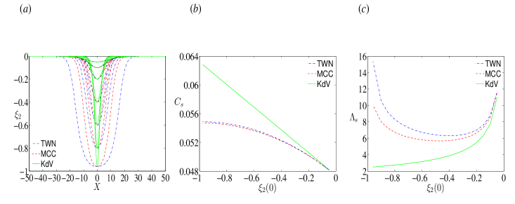
Figure 13: (Colour online) (a) Interfacial solitary-wave solutions of the TWN model (blue dashed-dotted line – $\cdot$ – $\cdot$ –), the MCC model (red dashed lines –  –  –) (Choi & Camassa, 1999), and the KdV model (green solid lines ———) (Choi & Camassa, 1999) with the same amplitude. As the amplitude increases, the solitary-wave solutions of both TWN and MCC models broaden and eventually develop a flat crest when the amplitude increases to approximately $(h_{1}-h_{2})/2$. (b) Velocity $C_{s}$ versus wave amplitude $\xi_{2}(0)$. There is good agreement of velocity between the TWN model and MCC model. (c) Effective width $\Lambda_{s}$ versus wave amplitude $\xi_{2}(0)$. There is qualitatively good agreement of effective width between the TWN model and MCC model.

To quantify the trend of wavelength broadening, we introduce a measure of the effective width, $\Lambda_{s}$, for the interfacial solitary wave solution (Koop & Butler, 1981):

$$\Lambda_{s}=\left|\frac{1}{\xi_{2}(0)}\int_{0}^{\infty}\xi_{2}(X)dX\right|.$$ (50)

For the effective width of the MCC and KdV solutions, one can refer to the reference (Choi & Camassa, 1999). Figure 13(c) displays the effective widths among TWN solutions, MCC solutions, and KdV solutions. For small-amplitude waves, there is good agreement of effective widths among the three models. However, discrepancies grow rapidly with the increase of the wave amplitude. Note that in this work, we focus more on the qualitative behavior of SWs instead of IWs. For IWs, the key point here is that our TWN model, MCC-type model, and the Hamiltonian model by Guyenne (2006) can capture the broadening of IWs as can be seen in the ocean (Duda et al., 2004) while the KdV model cannot.

Appendix C Numerical method and low-pass filter

Here, we present some details pertaining to our numerical computation. Throughout the text, the variables are all dimensionless. For the parameter regime I [$(h_{1},h_{2},g,\rho_{1},\rho_{2})=(1,3,1,1,1.003)$], we use $2^{15}$ uniformly distributed grid points for the numerical examples. We set the computational domain to be $[-M,M]$, with $M=300$. At the boundaries $X=-M$ and $X=M$, we use periodic boundary conditions. For the numerical examples in §§ 3.1 and § 4, we find that even for an initially narrowly localized short-mode wave perturbation, radiation is quickly emitted from the near field towards the boundaries $X=-M$ and $X=M$. To eliminate possible reflected waves from these boundaries, we establish two buffer zones in the regions $[-M,-M+m]$ and $[M-m,M]$ ($m\ll M$) where we add damping and diffusion terms to absorb the outgoing radiation. For the parameter regime II [$(h_{1},h_{2},g,\rho_{1},\rho_{2})=(1,5,1,0.856,0.996)$], we use $5\times 2^{13}$ grid points and domain with $M=375$. For our numerical scheme, we use the fourth-order Runge-Kutta method in time and the collocation method in space (Chen, 2005). We have numerically examined the accuracy of this scheme for the interfacial solitary wave solution. We use the $2/3$-rule for de-aliasing and a low-pass filter to suppress the Kelvin-Helmholtz instability as discussed below.

Figure 14: (Colour online) (a) The phase portrait of the short-mode wave-packet motion on the BBF in equation (26). Along each curve, the frequency $\overline{\nu}_{k}$ remains constant, with its value color-coded. Inside the region enclosed by the blue level-curve, the short-mode waves are trapped. The arrows indicate the direction of the wave-packet movement. Inside the black region, the frequency $\overline{\nu}_{k}$ is not real-valued, i.e., the mTWN model suffers from the KH instability in this region. (b) The phase portrait of the short-mode wave-packet motion corresponding to an underlying interfacial solitary wave with the amplitude $0.976$. Inside the two black regions, the mTWN model suffers from the KH instability. (c) Snapshots of SWs’ profile $\xi_{1}$ at $T=0$ and $T=80$, when the low-pass filter is not applied in the simulation. (d) Time evolution of SWs’ wavenumber spectrum $|\widehat{\xi}_{1}(k,T)|^{2}$ when the low-pass filter is not applied in the simulation.

Next, we demonstrate that although our mTWN system suffers from the Kelvin-Helmholtz (KH) instability in the presence of the BBF (26), these unstable wavenumbers are relatively large and are outside the wavenumber domain in some of our examples. Hence, our numerical computation is still stable and does not suffer from the KH instability. Figure 14(a) reproduces the phase portrait of the wave-packet motion depicted in figure 3(a), but over a larger wavenumber $k$ range. In the black region, the frequency $\overline{\nu}_{k}$ is not real-valued so that our mTWN system suffers from the KH instability. One can observe that the KH instability occurs for wavenumbers $k>k_{\text{KH}}=170$. However, this critical wavenumber $k_{\text{KH}}$ is outside the wavenumber domain used in our computation. Thus, our computation is still numerically stable.

However, for large-amplitude interfacial solitary wave simulations, our numerical computation suffers from the KH instability. Figure 14(b) displays the phase portrait of the wave-packet motion on an interfacial solitary wave with the amplitude $0.976$. We can see that the KH instability occurs at the leading and trailing edges for wavenumbers $k$ greater than $k_{\text{KH}}=100$. We numerically simulate our model using $2^{16}$ uniformly spaced grid points. The results are shown in figures 14(c) and (d): the KH instability, as expected, occurs at the leading and trailing edges for wavenumbers $k$ greater than $k_{\text{KH}}=100$.

To suppress this KH instability, we adopt in our computation a low-pass filter as in (Jo & Choi, 2008). In particular, we inhibit the growth of waves with their wavenumbers greater than $k_{\text{KH}}=90$. To examine the validity of the low-pass filter, we compute the conservation of mass and momentum,

$$C_{\xi_{j}}(T)=\int\xi_{j}dX,\ \ \ C_{M_{j}}(T)=\int M_{j}dX,$$ (51)

and then measure the maximum relative errors,

$$\Delta C_{\xi_{j}}=\max_{T}\left|\frac{C_{\xi_{j}}(T)-C_{\xi_{j}}(0)}{C_{\xi_{j}}(0)}\right|,\text{ \ }\Delta C_{M_{j}}=\max_{T}\left|\frac{C_{M_{j}}(T)-C_{M_{j}}(0)}{C_{M_{j}}(0)}\right|.$$ (52)

In this implementation, the time step is $\Delta T=0.02$, the mesh size is $\Delta X=600/2^{16}$, and the total running time is $10000$. The low-pass filter is applied to all the variables $(\xi_{j},\overline{u}_{j})$ every $40$ time steps. Finally, our numerical results show that the maximum relative errors in conservation of $(\xi_{1},\xi_{2},\overline{u}_{1},\overline{u}_{2})$ are $2.8$E$-7$, $1.9$E$-7$, $2.7$E$-7$, and $1.4$E$-7$, respectively, that is, mass and momentum are conserved. After suppressing the KH instability, an interfacial solitary wave solution can propagate for a sufficiently long time [not shown here].

Appendix D KdV-Schrödinger model

As mentioned in the conclusions and discussion § 5, a particularly detailed prior effort of modeling IW surface signature phenomena was undertaken in (Craig et al., 2012). In this appendix, we compare the model of (Craig et al., 2012) with ours. In (Craig et al., 2004, 2005, 2011, 2012), by applying perturbation analysis and canonical transformations to a Hamiltonian formulation of the two-layer Euler system, a resonantly-coupled system composed of a Korteweg–de Vries (KdV) equation for the long-mode waves and a linear Schrödinger equation (with an internal soliton as its potential well) for the short-mode waves was constructed. Narrow rough regions were found and interpreted as a result of the accumulation of energy in the localized bound states of the Schrödinger equation.

We also observe the accumulation of SW energy in our numerical results as shown in figures 9 and 11. Thus, our numerical results are consistent with the theory of energy accumulation for short SWs developed in (Craig et al., 2012). This property of energy accumulation is important for the generation of only one dominant wave packet [figure 11], which may be responsible for the narrow band of roughness generated by an IW as seen in many field observations (Gargett & Hughes, 1972; Osborne & Burch, 1980; Kropfli et al., 1999).

However, there exist two significant differences in the understanding of the surface signature between our work and (Craig et al., 2012). The first is the location of the surface ripples. In (Craig et al., 2012), due to the symmetry of the potential well (internal soliton) in the linear Schrödinger equation, the surface ripples are located at the crest of the internal soliton. In contrast, our work shows that due to the three types of asymmetric behavior of SWs [1a]- [1c] (linear modulation theory), a sink of SW packets is formed at the leading edge. These SWs can eventually accumulate at the leading edge due to the class 3 triad resonance. The second is the dynamical behavior of SWs in wavenumber $k$ space. In (Craig et al., 2012), due to the resonance condition (19), the coupled KdV-Schrödinger equation may only be valid for quasi-monochromatic surface waves near the resonant $k_{\text{res}}$. However, we numerically show that, for a wide range of wavenumbers, energy can eventually be concentrated near the resonant $k_{\text{res}}$ due to the modulation-resonance mechanism [see figure 12(b)]. These resonant surface wave packets can then propagate for a long time.

From the field observations, Osborne & Burch (1980) observed that, after the passage of surface ripples, the sea surface becomes completely calm, like a mill pond [the ‘mill pond’ effect]. For this ‘mill pond’ effect, Craig et al. (2012) pointed out that the passage of an internal soliton reflects the waves propagating in front of it, effectively sweeping the surface of waves, and resulting in the observed calmness of the sea after its passage. For the ‘mill pond’ effect, we present our hypothesis as follows: In the moving frame, the small-amplitude SW packets with $k>k_{\text{res}}$ in front of the leading edge [rightmost black arrows in figure 3] propagate towards the leading edge with a relatively small group velocity as predicted by the linear modulation theory. Once colliding with the large-amplitude dominant wave packet at the leading edge, these high-wavenumber ($k>k_{\text{res}}$), small-amplitude SW packets may be absorbed into the dominant wave packet. Therefore, in the rest frame, after the passage of an internal soliton, waves with $k>k_{\text{res}}$ in front of the leading edge may be absorbed into the dominant wave packet. Due to very few waves with $k>k_{\text{res}}$ traveling behind the dominant wave packet (which is always located at the leading edge), the ‘mill pond’ effect may be formed after the passage of an IW. However, due to the complicated set-up for the boundary condition on the right-hand side of the computational domain in front of the leading edge, it remains difficult to examine our hypothesis at this stage.

Finally, dissipation may play an important role in the surface signature. Since the typical wavelength of accompanying SWs is only about $0.1$-$1$ m for the underlying $1$ km internal soliton, these short SWs should be dissipated quickly by the viscosity, within at most a few hours. However, being generated by tidal flow, IWs usually can propagate thousands of kilometers with the accompanying SWs. This, on the other hand, implies that these accompanying SWs may accumulate energy from the background environment as pointed out in (Craig et al., 2012) and our work.

References

- Alam (2012) Alam, M.-R. 2012 A new triad resonance between co-propagating surface and interfacial waves. J. Fluid Mech. 691, 267–278.
- Alford et al. (2015) Alford, M. H., Peacock, T., MacKinnon, J. A., Nash, J. D., Buijsman, M. C., Centuroni, L. R., Chao, S.-Y., Chang, M.-H., Farmer, D. M., Fringer, O. B. & others 2015 The formation and fate of internal waves in the south china sea. Nature 521 (7550), 65–69.
- Alpers (1985) Alpers, W. 1985 Theory of radar imaging of internal waves. Nature 314 (6008), 245–247.
- Apel et al. (2007) Apel, J. R., Ostrovsky, L. A., Stepanyants, Y. A. & Lynch, J. F. 2007 Internal solitons in the ocean and their effect on underwater sound. J. Acoust. Soc. Amer. 121 (695 C722).
- Bakhanov & Ostrovsky (2002) Bakhanov, V. V. & Ostrovsky, L. A. 2002 Action of strong internal solitary waves on surface waves. J. Geophys. Res. 107 (3139).
- Barros & Choi (2009) Barros, R. & Choi, W. 2009 Inhibiting shear instability induced by large amplitude internal solitary waves in two-layer flows with a free surface. Stud. Appl. Math 122 (325-346).
- Barros & Gavrilyuk (2007) Barros, R. & Gavrilyuk, S. 2007 Dispersive nonlinear waves in two-layer flows with free surface part ii. large amplitude solitary waves embedded into the continuous spectrum. Stud. Appl. Math 119 (213-251).
- Benney (1977) Benney, D. 1977 A general theory for interactions between short and long waves. Stud. Appl. Math 56 (1), 81–94.
- Caponi et al. (1988) Caponi, E. A., Crawford, D. R., Yuen, H. C. & Saffman, P. G. 1988 Modulation of radar backscatter from the ocean by a variable surface current. Tech. Rep.. DTIC Document.
- Chen (2005) Chen, T. 2005 An efficient algorithm based on quadratic spline collocation and finite difference methods for parabolic partial differential equations. PhD thesis, University of Toronto.
- Choi et al. (2009) Choi, W., Barros, R. & Jo, T.-C. 2009 A regularized model for strongly nonlinear internal solitary waves. J. Fluid Mech. 629 (73-85).
- Choi & Camassa (1996) Choi, W. & Camassa, R. 1996 Weakly nonlinear internal waves in a two-fluid system. J. Fluid Mech. 313 (83-103).
- Choi & Camassa (1999) Choi, W. & Camassa, R. 1999 Fully nonlinear internal waves in a two-fluid system. J. Fluid Mech. 396 (1-36).
- Craig et al. (2004) Craig, W., Guyenne, P. & Kalisch, H. 2004 A new model for large amplitude long internal waves. C. R. Mecanique 332 (525-530).
- Craig et al. (2005) Craig, W., Guyenne, P. & Kalisch, H. 2005 Hamiltonian long wave expansions for free surfaces and interfaces. Commun. Pure Appl. Maths 58 (1587-1641).
- Craig et al. (2011) Craig, W., Guyenne, P. & Sulem, C. 2011 Coupling between internal and surface waves. Nat. Hazards 57 (617-642).
- Craig et al. (2012) Craig, W., Guyenne, P. & Sulem, C. 2012 The surface signature of internal waves. J. Fluid Mech. 710 (277-303).
- Donato et al. (1999) Donato, A. N., Peregrine, D. H. & Stocker, J. R. 1999 The focusing of surface waves by internal waves. J. Fluid Mech. 384, 27–58.
- Duda & Farmer (1999) Duda, T. F. & Farmer, D. M. 1999 The 1998 WHOI/IOS/ONR Internal Solitary Wave Workshop: Contributed Papers. Tech. Rep.. DTIC Document.
- Duda et al. (2004) Duda, T. F., Lynch, J. F., Irish, J. D., Beardsley, R. C., Ramp, S. R., Chiu, C. S., Tang, T. Y. & Yang, Y. J. 2004 Internal tide and nonlinear wave behavior in the continental slope in the northern south china sea. IEEE J. Ocean. Eng. 29 (1105-1131).
- Dysthe et al. (2008) Dysthe, K., Krogstad, H. E. & Müller, P. 2008 Oceanic rogue waves. Annu. Rev. Fluid Mech. 40, 287–310.
- Funakoshi & Oikawa (1983) Funakoshi, M. & Oikawa, M. 1983 The resonant interaction between a long internal gravity wave and a surface gravity wave packet. J. Phys. Soc. Jpn 56 (1982-1995).
- Gargett & Hughes (1972) Gargett, A. E. & Hughes, B. A. 1972 On the interaction of surface and internal waves. J. Fluid Mech. 52 (01), 179–191.
- Gasparovic et al. (1988) Gasparovic, R. F., Apel, J. R. & Kasischke, E. S. 1988 An overview of the sar internal wave experiment. J. Geophys. Res. 93 (12,304-12,316).
- Guyenne (2006) Guyenne, P. 2006 Large-amplitude internal solitary waves in a two-fluid model. Comptes Rendus Mécanique 334 (6), 341–346.
- Han & Xu (2007) Han, H. & Xu, Z. 2007 Numerical solitons of generalized korteweg cde vries equations. Appl. Math. Comput. 186 (483-489).
- Hashizume (1980) Hashizume, Y. 1980 Interaction between short surface waves and long internal waves. J. Phys. Soc. Jpn 48 (631-638).
- Hwung et al. (2009) Hwung, H.-H., Yang, R.-Y. & Shugan, I. V. 2009 Exposure of internal waves on the sea surface. J. Fluid Mech. 626 (1-20).
- Jo & Choi (2008) Jo, T.-C. & Choi, W. 2008 On stabilizing the strongly nonlinear internal wave model. Stud. Appl. Math 120 (65-85).
- Johnston et al. (2003) Johnston, T. S., Merrifield, M. A. & Holloway, P. E. 2003 Internal tide scattering at the line islands ridge. J. Geophys. Res. 108 (C11).
- Kawahara et al. (1975) Kawahara, T., Sugimoto, N. & Kakutani, T. 1975 Nonlinear interaction between short and long capillary-gravity waves. J. Phys. Soc. Jpn. 39 (5), 1379–1386.
- Kodaira et al. (2016) Kodaira, T., Waseda, T., Miyata, M. & Choi, W. 2016 Internal solitary waves in a two-fluid system with a free surface. J. Fluid Mech. 804, 201–223.
- Koop & Butler (1981) Koop, C. G. & Butler, G. 1981 An investigation of internal solitary waves in a two-fluid system. J. Fluid Mech. 112, 225–251.
- Kropfli et al. (1999) Kropfli, R. A., Ostrovski, L. A., Stanton, T. P., Skirta, E. A., Keane, A. N. & Irisov, V. 1999 Relationships between strong internal waves in the coastal zone and their radar and radiometric signatures. J. Geophys. Res. 104 (3133-3148).
- Lee et al. (2007) Lee, K.-J., Shugan, I. V. & An, J.-S. 2007 On the interaction between surface and internal waves. J. Korean Phys. Soc. 51 (616-622).
- Lewis et al. (1974) Lewis, J. E., Lake, B. M. & Ko, D. R. S. 1974 On the interaction of internal waves and surface gravity waves. J. Fluid Mech. 63 (04), 773–800.
- Moore & Lien (2007) Moore, S. E. & Lien, R.-C. 2007 Pilot whales follow internal solitary waves in the south china sea. Mar. Mamm. Sci. 23 (1), 193–196.
- Müller et al. (2005) Müller, P., Garrett, C. & Osborne, A. 2005 Rogue waves. Oceanography 18 (3), 66.
- Osborne & Burch (1980) Osborne, A. R. & Burch, T. L. 1980 Internal solitons in the andaman sea. Science 208 (451-460).
- Parau & Dias (2001) Parau, E. & Dias, F. 2001 Interfacial periodic waves of permanent form with free-surface boundary conditions. J. Fluid Mech. 437 (325-336).
- Perry & Schimke (1965) Perry, R. B. & Schimke, G. R. 1965 Large-amplitude internal waves observed off the northwest coast of sumatra. J. Geophys. Res. 70 (10), 2319–2324.
- Phillips (1966) Phillips, O. M. 1966 The Dynamics of the Upper Ocean. Cambridge University Press.
- Phillips (1974) Phillips, O. M. 1974 Nonlinear dispersive waves. Annu. Rev. Fluid Mech. 6 (93-110).
- Sepulveda (1987) Sepulveda, N. 1987 Solitary waves in the resonant phenomenon between a surface gravity wave packet and an internal gravity wave. Phys. Fluids 30 (7).
- Tanaka & Wakayama (2015) Tanaka, M. & Wakayama, K. 2015 A numerical study on the energy transfer from surface waves to interfacial waves in a two-layer fluid system. J. Fluid Mech. 763, 202–217.
- Whitham (1974) Whitham, G. B. 1974 Linear and Nonlinear Waves. A Wiley-Interscience Publication, New York.