Delay lines test method for the Blade Template

Abstract

This paper proposes a method for testing the delay lines of Blade asynchronous timing resilience template. It consists of an offline test method, with low area overhead, for measuring the internal propagation delay of the delay lines with external testers.

I Introduction

Asynchronous bundled-data designs, in general, must incorporate delay lines in their control signals to compensate for data path propagation through computational logic. The correctness of delay lines is crucial for the system to work correctly. However, the delay lines are subject to variability and faults.

In bundled-data designs, the circuit is faulty if the data path becomes slower or if the delay lines become faster than the timing specifications. In the literature, there are not many works that address the testability of delay lines in bundled-data designs. The work of Sato [1] relies on scannable data path and two-pattern delay test methodology to measure the delay of the combinational block, thus the method does not take delay measurements of the delay lines itself. Timing information is captured by a time to digital converter and used later to configure the delay lines to a value that is long enough to compensate for the data path delay. Moreover, applying Sato’s [1] approach would incur in significant area overhead due to the need of a scannable data path.

Blade [2] is an asynchronous bundled-data template with timing resilience capabilities, that can recover from timing violation in the data path. Blade relies on the delay lines as a timing reference to detect the timing violations. So, this paper proposes a method for testing Blade’s delay lines. It consists of an offline test method for measuring the propagation delay of the delay lines of the manufactured circuit. The results show that the method has low area overhead and a simple DfT circuitry. On the other hand, it requires an accurate external tester to precisely measure the delay of the delay lines via external pins.

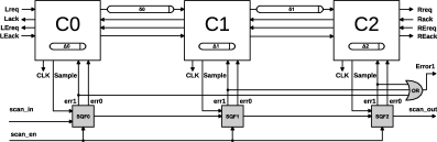
Figure 1: Delay lines test scenario with Blade design.

II Proposed Method

The proposed method aims to use only primary inputs and outputs to take delay measurements, which include the handshake protocol pins (L/R channel and LE/RE channel) and an additional pin that serves as an observation point for the err1 signals, as illustrated in Fig. 1. Besides that, a scan chain to add controllability over the Q-Flops state is assumed. As previously discussed, a scannable data path is undesired due to high area overheads, but instead, the proposed method assumes the replacement of Q-Flops for Scan Q-Flops (SQF) [3], which represents a smaller number of scan elements than a full scan. For instance, a 32 bit Blade [2] stage requires 4 SQFs. The SQF is mandatory for the proposed test method since the Q-Flop acts as a metastability filter, and there is an unbounded time for metastability to be resolved inside the Q-Flop filter and settle the correct output error signal. With the SQF, this time uncertainty no longer exists, and correct timing assumptions can be made for the proposed test method.

II-A Test Architecture

Fig. 1 shows a simplified 3-stage pipeline example of the architecture. In this scenario, the left channels of C0 and the right channels of C2 are connected to primary inputs and outputs, and a single SQF representation is presented. Through the proposed scan chain err1 and err0 can be forced to a controlled state immediately after Sample rises. Internal err1 signals are grouped with an OR gate, and its output is mapped to a primary output pin called Error1. This design allows delay measurement of the err1 rising moment for the different stages. For instance, if SQF1 is configured to raise its err1 output signal, and all the others to rise their err0 signal, the rising edge observed at the primary output corresponds to the err1 connected to controller C1, assuming no fault at the OR gate.

The proposed Blade controller [2] implements the handshake protocol assuming two $\Delta$ delay lines and their consolidation into a single one is left for future works. For our test method, we assume that the $\Delta$ delay line is a single delay element. Nevertheless, the proposed test method could be extended for testing controllers with different internal delay lines such as Sharp [4]. However, further analyses are required as the handshake protocol is different, and the time measurements need to be derived and measured from different pins and internal observation points. Accordingly, this is left for future work, along with an extension to consider forks and joins.

II-B Test Procedure

Some important aspects of the controller and the implemented communication protocol must be described for a better understanding of the test procedure. The $\Delta$ delay line controls the high phase of CLK and $\delta$ delay line is equivalent to the longest path of the combinational logic between the pipeline stages. A request arriving at the primary input Lreq is immediately forwarded from the left channel to the right channel connected to C0. This means that if no timing violations are flagged (only err0 rises), and the pipeline is empty, the time from Lreq to Rreq is equal to the sum of all $\delta$ delay lines propagation ($\delta 0$, $\delta 1$ and $\delta 2$). Another thing to notice is that at the same time that Lreq is flagged, internally the CLK signal rises and the $\Delta$ delay line is activated.

After the high phase of CLK the Sample signal rises, and err0 or err1 are immediately flagged, which is possible with the use of the SQF previously configured through the scan chain. In this case, it is possible to assume that the time from Lreq to err1 or err0 is equal to the $\Delta$ delay line propagation, thus both can be used as an observation point to measure the $\Delta$ delay. However, err1 activates the protocol extension phase, which is required for measuring the $\delta$ delay, so err1 has been selected because it serves both tests.

One last thing to mention is that the REack is the protocol signal that indicates that all delay lines ended their signal propagation, regardless of which error signal was flagged. Now it is possible to describe the test steps and the equations used to calculate the propagation delay of all delay lines in a circuit implemented with Blade. Between each step, the circuit goes through a complete reset.

• Step 1: The first delay measurement corresponds to the sum of all $\delta$ delays. All SQFs are configured to raise their err0 output signal and the communication is started at the left channel. Equation 1 defines that the sum of all $\delta$ delays is the difference time between the first Lreq transition ($T_{Lreq}$) and the first Rreq transition ($T_{Rreq}$) that arrives at the end of the pipeline.

$$T_{Sum}=T_{Rreq}-T_{Lreq}$$ (1)

• Step 2: This step is repeated for each controller to take the delay measurement of the internal $\Delta$ delay line. For this test only the SQF connected to the target controller is configured to raise its err1 output signal. By forcing the delay extension, the pipeline propagation time is increased by the $\Delta$ delay. Equation 2 is used to calculate the $\Delta$ delay of each controller. The difference time between the first Lreq transition ($T_{Lreq}$) and the first REack transition ($T_{REack}$) that arrives at the end of the pipeline, minus the sum of all $\delta$ delays calculated in the previous step, is equal to the $\Delta$ delay of the target controller $i$.

$$\Delta_{i}=T_{REack}-T_{Lreq}-T_{Sum}$$ (2)

• Step 3: The last step is used for measuring the $\delta$ delay lines between controllers. This step is repeated for each $\delta$ delay line. For this test the SQF connected to the controller that follows the target delay line is configured to rise the err1 signal, and the transition observed in Error1 corresponds to this SQF. Equation 3 is used to calculate the $\delta$ delay between each each stage. The target $\delta$ delay $i$ is given by the difference time between the first Lreq transition ($T_{Lreq}$) and the first Error1 transition ($T_{Error1}$), minus the sum of $\delta$ delays previously calculated in this current step, minus the $\Delta$ delay of the controller that follows the target delay line ($i+1$). This last subtraction accounts for the fact that the $i+1$ err1 only rises after the high phase of CLK, which is controlled by the $\Delta_{i+1}$.

$$\delta_{i}=T_{Error1}-T_{Lreq}-(\sum_{k=0}^{i-1}\delta_{k})-\Delta_{i+1}$$ (3)

III Preliminary Results

An RTL description of the pipeline presented in Fig. 1 was used for validation of the proposed test procedure and equations, and all the delays were correctly extracted. For these tests only the delays lines had propagation delay values.

The estimated area of the system described in Fig. 1 is $Area=N*(A_{control}+A_{Qflop})+A_{NinOR}$, where it represents the area of the controller, the SQF cell, and the N-input OR gate, respectively. N is the number of pipeline stages. The delay line area is excluded since it is dependent on the design. Assuming a fabrication technology of $28\text{\,}\mathrm{nm}$, the original Q-Flop has an area of about $7\text{\,}{\mathrm{\SIUnitSymbolMicro m}}^{2}$ with 28 transistors, while the SQF cell has an area of $10\text{\,}{\mathrm{\SIUnitSymbolMicro m}}^{2}$ with 40 transistors. The controller presents an area of $27\text{\,}{\mathrm{\SIUnitSymbolMicro m}}^{2}$, and the OR presents an area of $2.6\text{\,}{\mathrm{\SIUnitSymbolMicro m}}^{2}$. Thus, for the scenario presented in Fig. 1, the total area is $113.6\text{\,}{\mathrm{\SIUnitSymbolMicro m}}^{2}$, while the area without the test (i.e. using the Q-Flop cell) is $102\text{\,}{\mathrm{\SIUnitSymbolMicro m}}^{2}$, representing an overhead of 11.37%.

IV Conclusions

This paper proposed a method for testing the delay lines of Blade. The method correctly extracts the Blade’s delay lines values and presents a low area overhead of 11.37%. The next step is to apply the proposed method to a mapped netlist in order to account for additional propagation delays and the related error introduced in the time measurements.

References

- [1] S. Sato and S. Ohtake, “A delay measurement mechanism for asynchronous circuits of bundled-data model,” in DDECS, 2015, pp. 243–248.
- [2] D. Hand et al., “Blade – a timing violation resilient asynchronous template,” in ASYNC, 2015, pp. 21–28.
- [3] L. R. Juracy et al., “A DfT insertion methodology to scannable Q-Flop elements,” IEEE TVLSI Systems, vol. 26, no. 8, pp. 1609–1612, 2018.
- [4] M. Waugaman and W. Koven, “Sharp - a resilient asynchronous template,” in ASYNC, 2017, pp. 83–84.