Unitarity of the infinite-volume three-particle scattering amplitude
arising from a finite-volume formalism

Abstract

In Ref. Hansen and Sharpe (2015), two of us derived a relation between the scattering amplitude of three identical bosons, $\mathcal{M}_{3}$, and a real function referred to as the divergence-free K matrix and denoted ${\mathcal{K}_{\mathrm{df},3}}$. The result arose in the context of a relation between finite-volume energies and ${\mathcal{K}_{\mathrm{df},3}}$, derived to all orders in the perturbative expansion of a generic low-energy effective field theory. In this work we set aside the role of the finite volume and focus on the infinite-volume relation between ${\mathcal{K}_{\mathrm{df},3}}$ and $\mathcal{M}_{3}$. We show that, for any real choice of ${\mathcal{K}_{\mathrm{df},3}}$, $\mathcal{M}_{3}$ satisfies the three-particle unitarity constraint to all orders. Given that ${\mathcal{K}_{\mathrm{df},3}}$ is also free of a class of kinematic divergences, the function may provide a useful tool for parametrizing three-body scattering data. Applications include the phenomenological analysis of experimental data (where the connection to the finite volume is irrelevant) as well as calculations in lattice quantum chromodynamics (where the volume plays a key role).

I Introduction

Three-body systems lie at the forefront of modern-day theoretical hadronic physics. Whether in the context of understanding the resonance spectrum of quantum chromodynamics (QCD) or the binding of nucleons in nuclei, three-body dynamics play a crucial role. In recent years there has been significant progress in developing rigorous theoretical frameworks for studying such systems.

The majority of QCD states are unstable resonances that decay via the strong force into multihadron configurations. A quantitative description of these is given by identifying complex-valued energy poles in the scattering amplitudes of the resonance decay products. Given that one can only access real-valued energies experimentally, it is necessary to construct amplitude parametrizations that can be analytically continued into the complex energy plane, in order to determine the pole positions. Since resonance widths originate from the presence of open decay channels, unitarity plays a key role in the analytic continuation. It is straightforward to impose unitarity on two-body amplitudes, but it far more challenging in the three-body case, with efforts dating back to the 1960s Bjorken (1960); Aitchison and Pasquier (1966); Ascoli and Wyld (1975).

The availability of high-precision data on various three-body production and resonance decay channels, together with the emergence of lattice QCD (LQCD) calculations of hadron scattering, has reignited interest in the three-body problem Magalhaes et al. (2011); Mai et al. (2017); Mikhasenko et al. (2019); Jackura et al. (2018). Although unitarity gives a powerful restriction on the structure of scattering amplitudes, it does not fully determine them. The unconstrained real part, often referred to as the K matrix, is determined by the underlying microscopic theory, and in practice is obtained by fitting to experimental data or LQCD finite-volume spectra. By comparing results obtained with different K-matrix parametrizations it is possible to determine the existence of amplitude singularities and learn about their microscopic origin. This approach has proven remarkably powerful, not only for the determination of simple QCD observables, but also in multiparticle quantities including scattering and transition amplitudes.

In LQCD, using the standard approach, one can directly access only the eigenstates and energies of the finite-volume Hamiltonian, which are not in direct correspondence to multiparticle asymptotic states. This prevents a direct determination of S-matrix elements. Nevertheless, it turns out that one can extract scattering information via model-independent relations between finite- and infinite-volume quantities. For two-particle systems there has been a great deal of progress in developing such formalism, culminating in a general relation between the finite-volume spectrum of any coupled two-particle system and its corresponding scattering matrix Lüscher (1986, 1991); Rummukainen and Gottlieb (1995); Kim et al. (2005); He et al. (2005); Lage et al. (2009); Fu (2012); Hansen and Sharpe (2012); Briceño and Davoudi (2013a); Göckeler et al. (2012); Briceño (2014). In addition, relations have been derived between finite-volume matrix elements and the corresponding transition amplitudes mediated by an external current Lellouch and Lüscher (2001); Christ et al. (2005); Meyer (2011); Bernard et al. (2012); Agadjanov et al. (2014); Briceño et al. (2015); Feng et al. (2015); Briceño and Hansen (2015, 2016); Baroni et al. (2018). These relations, along with algorithmic advances, have made possible the study of resonant and non-resonant scattering amplitudes of various two-body channels Wilson et al. (2015); Briceño et al. (2017); Brett et al. (2018); Guo et al. (2018); Andersen et al. (2018, 2019) including energies where more than one channel is open Dudek et al. (2014, 2016); Woss et al. (2018, 2019). We point the reader to Ref. Briceño et al. (2018a) for a recent review of the formalism and its implementation.

Presently, the extension of these studies to energies above three-particle thresholds is limited as the required three-body finite-volume formalism is still under development, although finite-volume energy levels coupling to three-particle states are already being extracted using lattice QCD Beane et al. (2013); Cheung et al. (2017); Woss et al. (2019); Detmold and Nicholson (2013); Hörz and Hanlon (2019). The need for this extension has motivated several efforts Polejaeva and Rusetsky (2012); Briceño and Davoudi (2013b); Hansen and Sharpe (2014, 2015); Hammer et al. (2017a, b); Guo and Gasparian (2017); Mai and Döring (2017); Briceño et al. (2017); Döring et al. (2018); Briceño et al. (2018b); Mai and Döring (2019); Briceño et al. (2019); Blanton et al. (2019), which were recently reviewed in Ref. Hansen and Sharpe (2019). At this stage, the formal approach is complete for systems of three identical scalar particles, including systems with two-to-three transitions as well as those with a resonant two-particle subprocess.

In this article we restrict attention to the formalism introduced by two of us in Refs. Hansen and Sharpe (2014, 2015). This approach, derived via an all-orders perturbative expansion of a generic scalar field theory, relates finite-volume energy levels to an intermediate infinite-volume quantity referred to as the three-body divergence-free K matrix, and denoted $\mathcal{K}_{\text{df},3}$. In a second step this real-valued intermediate quantity is related, using a set of known integral equations, to the complex valued three-to-three scattering amplitude, $\mathcal{M}_{3}$. Qualitatively, one can understand $\mathcal{K}_{\text{df},3}$ as the part of the scattering amplitude that describes all of the microscopic interactions between the three particles that remain after the explicit effects of particle exchanges are subtracted. This is somewhat analogous to the relation between the real-valued K matrix and the complex scattering amplitude in the two-particle sector, reviewed in Sec. II below.

In this work we set aside the role of the finite-volume and consider the implications of the relation between ${\mathcal{K}_{\mathrm{df},3}}$ and $\mathcal{M}_{3}$. We demonstrate, to all orders in a $\mathcal{K}_{\text{df},3}$ expansion, that any scattering amplitude expressed in terms of this real-valued quantity exactly satisfies three body unitarity. We stress here that the formulation is fully relativistic and incorporates all partial waves in the three-particle system as well as its two-particle subsystems. We do, however, restrict attention to the relations of Ref. Hansen and Sharpe (2015), meaning that the expressions describe a single channel of three identical scalars.

We stress that our result is expected, since the derivation of the expression for $\mathcal{M}_{3}$ in terms of ${\mathcal{K}_{\mathrm{df},3}}$ is based on an all-orders analysis in quantum field theory. Nevertheless, since the derivation is complicated and lengthy, our result provides an important cross check of the final expression. In addition, we hope that our result stimulates comparison of the unitary expression for $\mathcal{M}_{3}$ in terms of ${\mathcal{K}_{\mathrm{df},3}}$ with other unitary parametrizations, such as that of Refs. Mai et al. (2017); Jackura et al. (2018).

The remainder of this work is organized as follows. In Sec. II, in addition to introducing some basic notation, we review the definition of the scattering amplitude in terms of the K matrix in both the two- and three-particle sectors. Next, in Sec. III, we review the unitarity relation, with some details relegated to the appendix, and demonstrate that $\mathcal{M}_{3}[\mathcal{K}_{\text{df},3}]$ exactly satisfies the constraining equation. The derivation proceeds in two steps, first showing that the relation holds for ${\mathcal{K}_{\mathrm{df},3}}=0$ and then incorporating the all-orders effects of the local three-body interaction. We conclude briefly in Sec. IV.

II Two- and three-body scattering

In this section we set up some of the notation and key relations used in this work to describe both two- and three-particle scattering. First, in the following subsection, we introduce the two-particle scattering amplitude and recall how its relation to the K matrix automatically satisfies unitarity. Then, in Sec. II.2, we give the relation between the fully-connected three-particle scattering amplitude, $\mathcal{M}_{3}$, and ${\mathcal{K}_{\mathrm{df},3}}$. In this case both the unitarity constraint and the relation between K matrix and scattering amplitude are more complicated. However, as we show in Sec. III, any form of $\mathcal{M}_{3}$ defined in terms of a real-valued ${\mathcal{K}_{\mathrm{df},3}}$ will satisfy the unitarity constraint.

Figure 1: The two types of contribution to the three-particle T matrix. $\mathcal{M}_{3}$ is the fully-connected amplitude.

II.1 Two-body scattering amplitude

The three-body T matrix, illustrated in Fig. 1, is defined in terms of the S matrix as $iT=S-1$. It has a disconnected contribution, depicted as the first term on the right hand side of the figure, in which two particles scatter without interacting with the third, spectator, particle. As one would expect, this contribution is fully determined by the two-particle scattering amplitude, denoted $\mathcal{M}_{2}$. To give a useful expression for this, we first define $\mathbf{k}$ as the momentum of the spectator particle in some arbitrarily chosen frame. The 4-momentum of this particle is then $(\omega_{k},\mathbf{k})$ where $\omega_{k}=\sqrt{\mathbf{k}^{2}+m^{2}}$ and $m$ is the physical mass. We further define the total three-particle energy and momentum in this frame to be $(E,\mathbf{P})\equiv P^{\mu}$. Thus, if we take one of the incoming scattering particles to carry four-momentum $(\omega_{a},\mathbf{a})$, then the second incoming scatterer will have $(E-\omega_{k}-\omega_{a},\mathbf{P}-\mathbf{k}-\mathbf{a})$.

Note that, by enforcing a specific value of total 4-mometum, $(E,\mathbf{P})$, we have given the second scattering particle an energy and momentum that do not necessarily satisfy the on-shell condition. To add this constraint, we need to introduce some new notation. Define

$$E_{2,k}^{\star}\equiv\sqrt{(E-\omega_{k})^{2}-(\mathbf{P}-\mathbf{k})^{2}}\,,$$ (1)

as the energy of the two scattering particles in their center-of-mass frame. In other words, the 4-vector $(E-\omega_{k},\mathbf{P}-\mathbf{k})$ boosts to $(E_{2,k}^{\star},\mathbf{0})$. Denoted by $(\omega_{a}^{\star},\mathbf{a}^{\star}_{k})$ is the result of applying this same boost to $(\omega_{a},\mathbf{a})$. It then directly follows that $(E-\omega_{k}-\omega_{a},\mathbf{P}-\mathbf{k}-\mathbf{a})$ is boosted to $(E_{2,k}^{\star}-\omega_{a}^{\star},-\mathbf{a}^{\star}_{k})$. We thus place the third particle on shell by requiring

$$E_{2,k}^{\star}-\omega_{a}^{\star}\overset{!}{=}\omega_{a}^{\star}\ \ \ \Longrightarrow\ \ \ a^{\star}_{k}\equiv|\textbf{a}^{\star}_{k}|\overset{!}{=}q_{k}^{\star}\equiv\sqrt{E_{2,k}^{\star 2}/4-m^{2}}\,.$$ (2)

Having enforced this condition we are left with the following (redundant) degrees of freedom for $\mathcal{M}_{2}$, viewed as the disconnected contribution to the three-particle T matrix: total 4-momentum [$P^{\mu}=(E,\mathbf{P})$], spectator momentum ($\mathbf{k}$), and incoming and outgoing directional freedom ($\widehat{\mathbf{a}}^{\star}_{k}$ and $\widehat{\mathbf{a}}^{\prime\star}_{k}$). This leads us to write the two-particle scattering amplitude as

$$\mathcal{M}_{2}(\mathbf{k},\widehat{\mathbf{a}}^{\prime\star}_{k};\mathbf{k},\widehat{\mathbf{a}}^{\star}_{k}) =4\pi Y_{\ell^{\prime}m^{\prime}}(\widehat{\mathbf{a}}^{\prime\star}_{k})\,\mathcal{M}_{2;\ell^{\prime}m^{\prime};\ell m}(\mathbf{k})\,Y^{*}_{\ell m}(\widehat{\mathbf{a}}^{\star}_{k})\,,$$ (3)

where $Y_{\ell m}$ are the standard spherical harmonics and the sum over repeated angular-momentum indices is implicit. We stress that $\widehat{\mathbf{a}}^{\star}_{k}$ and $\widehat{\mathbf{a}}^{\prime\star}_{k}$ are the spherical angles of the relative momenta between the two particles when the system recoils against the same spectator.

In what follows, we will be interested in determining the imaginary contributions to the two- and three-body scattering amplitudes. In doing so, one might have thought that it would be necessary to keep track of the imaginary parts of the spherical harmonics. Fortunately, it is easy to convince oneself that these contributions exactly vanish. In the case of $\mathcal{M}_{2}$ this follows from the fact that, as a result of Wigner-Eckart theorem, the two-body scattering scattering amplitude is diagonal, and independent of the azimuthal indices $m^{\prime}$ amd $m$

$$\mathcal{M}_{2;\ell^{\prime}m^{\prime};\ell m}(\mathbf{k})=\mathcal{M}^{(\ell)}_{2}(\mathbf{k})\,\,\delta_{\ell^{\prime}\ell}\delta_{m^{\prime}m}\,.$$ (4)

This implies that the product of the two harmonics in Eq. (3) reduces to the real Wigner-$d$ function, or equivalently the Legendre polynomial,

$$\sum_{m=-\ell}^{\ell}4\pi\,Y_{\ell m}(\widehat{\mathbf{a}}^{\prime\star}_{k})\,Y^{*}_{\ell m}(\widehat{\mathbf{a}}^{\star}_{k})=(2\ell+1)d^{\ell}_{00}\big{(}\widehat{\mathbf{a}}^{\prime\star}\cdot\widehat{\mathbf{a}}^{\star}\big{)}=(2\ell+1)P_{\ell}\big{(}\widehat{\mathbf{a}}^{\prime\star}\cdot\widehat{\mathbf{a}}^{\star}\big{)}\,,$$ (5)

for each $\ell$. An alternative argument is to note that it is legitimate to use real spherical harmonics, which form a complete set and satisfy the same orthonormality properties as the usual complex harmonics. Since the harmonics do not appear in the final expressions, we can use either basis in intermediate steps. For the real harmonics, the issue with the imaginary part does not arise. Since all other steps in the derivation have the same form in either basis, we will get the correct answer if we proceed as if the harmonics are real, even if we use the complex basis. This argument holds also in the analysis of the connected three-particle amplitude.

Given that $\mathcal{M}_{2;\ell^{\prime}m^{\prime};\ell m}$ is diagonal, keeping both pairs of indices may seem superfluous. However, as we will see below, it is convenient to think of this as a matrix in angular-momentum space, especially when combining it with other non-diagonal objects. To simplify the notation, in what follows we will largely leave the angular-momentum indices implicit.

We now define the real-valued two-particle K matrix, $\mathcal{K}_{2}$, via the standard relation

$$\mathcal{M}_{2}(\mathbf{k})^{-1}=\mathcal{K}_{2}(\mathbf{k})^{-1}+\rho(\mathbf{k})\,,$$ (6)

where $\rho$ is imaginary above threshold

$${\rm Im}\,\rho_{\ell^{\prime}m^{\prime};\ell m}(\mathbf{k})=-\delta_{\ell^{\prime}\ell}\delta_{m^{\prime}m}\Theta(q_{k}^{\star 2})\bar{\rho}(\mathbf{k}),\qquad\bar{\rho}(\mathbf{k})\equiv\frac{q_{k}^{\star}}{16\pi E_{2,k}^{\star}}\,.$$ (7)

Here we are using Eqs. (A6) and (A7) from Ref. Hansen and Sharpe (2015), with $\Theta(x)$ the usual Heaviside step function.

From these relations follows

$${\rm Im}\,\mathcal{M}_{2}(\mathbf{k})={\rm Im}\bigg{[}\frac{\mathcal{K}_{2}(\mathbf{k})^{-1}+\rho(\mathbf{k})^{*}}{\mathcal{K}_{2}(\mathbf{k})^{-1}+\rho(\mathbf{k})^{*}}\frac{1}{\mathcal{K}_{2}(\mathbf{k})^{-1}+\rho(\mathbf{k})}\bigg{]}=\mathcal{M}_{2}^{*}(\mathbf{k})\,\Theta(q_{k}^{\star 2})\,\bar{\rho}(\mathbf{k})\,\mathcal{M}_{2}(\mathbf{k})\,,$$ (8)

where we stress that the overall sign is positive. This result is equivalent to the standard unitarity relation, given in Eq. (106) in the Appendix. In order to compare to the literature on three-particle amplitudes, and in particular to Ref. Jackura et al. (2018), we note that the exact relation of our $\bar{\rho}$ to the corresponding quantity in that work is

$$4\pi\rho^{\text{Ref\,\cite[cite]{\@@bibref{Authors Phrase1YearPhrase2}{Jackura:2018xnx}{\@@citephrase{(}}{\@@citephrase{)}}}}}_{2k}=2\times\bar{\rho}(\mathbf{k})\,.$$ (9)

The factor of $4\pi$ arises because, in Ref. Jackura et al. (2018), the angular integral is left explicit [as shown in Eq. (36) below]. The factor of $2$ arises because of the symmetry factor which reduces the two-body phase space for identical particles.

We close this subsection by giving an alternative derivation of Eq. (8) that more closely matches the three-particle derivation of the following section. To do so we first expand the relation between $\mathcal{M}_{2}$ and $\mathcal{K}_{2}$ in powers of the latter

$$\mathcal{M}_{2}(\mathbf{k})=\sum_{n=0}^{\infty}\mathcal{K}_{2}(\mathbf{k})\big{[}-\rho(\mathbf{k})\mathcal{K}_{2}(\mathbf{k})]^{n}\,.$$ (10)

To evaluate the imaginary part in this form we introduce a general identity for a product of $n$ complex matrices

$${\rm Im}\,(A_{1}A_{2}\cdots A_{n})={\rm Im}\,(A_{1})A_{2}\cdots A_{n}+A_{1}^{*}\,{\rm Im}\,(A_{2})A_{3}\cdots A_{n}+\cdots+A_{1}^{*}\cdots A_{n-1}^{*}{\rm Im}\,(A_{n})\,.$$ (11)

This follows from simply substituting $2i\,{\rm Im}\,A_{j}=A_{j}-A_{j}^{*}$ and noting that terms cancel in pairs. The complex conjugation could occur also to the right of the ${\rm Im}(A_{j})$ factors, as can be trivially seen by conjugating both sides and using that $\text{Im}(x)$ is real.

Applying this identity to the $n$th term of Eq. (10) then gives

$${\rm Im}\Big{[}\mathcal{K}_{2}(\mathbf{k})\big{[}-\rho(\mathbf{k})\mathcal{K}_{2}(\mathbf{k})]^{n}\Big{]}=\sum_{m=0}^{n-1}\Big{(}\mathcal{K}_{2}(\mathbf{k})\big{[}-\rho(\mathbf{k})^{*}\mathcal{K}_{2}(\mathbf{k})]^{m}\Big{)}\ \Theta(q_{k}^{\star 2})\,\bar{\rho}(\mathbf{k})\ \Big{(}\mathcal{K}_{2}(\mathbf{k})\big{[}-\rho(\mathbf{k})\mathcal{K}_{2}(\mathbf{k})]^{n-m-1}\Big{)}\,,$$ (12)

where the right-hand side is understood to vanish for $n=0$ since then the sum contains no terms. Summing this result over all $n$ immediately gives Eq. (8). The intuition here is as follows: For a given series of real K matrices and complex valued $\bar{\rho}$ cuts, the identity (11) gives a prescription for moving through the chain, summing over all cuts with the conjugated object appearing to the left. Summing over all resulting terms then directly leads to the unitarity relation.

II.2 Three-body scattering amplitude

We now turn to the relevant expressions for the fully-connected three-particle scattering amplitude, $\mathcal{M}_{3}$, which is depicted in Fig. 1. The three-body scattering amplitude is naturally more complicated than $\mathcal{M}_{2}$. In Ref. Hansen and Sharpe (2015), it was shown in a bottom-up approach based on all-orders perturbation theory, that the scattering-amplitude is completely determined by a real function, denoted ${\mathcal{K}_{\mathrm{df},3}}$. This describes microscopic interactions between the three-particles, i.e. the part of the scattering amplitude that is not constrained by $s$-channel unitarity. For example, in the context of an effective field theory, it is given by a sum of contact interactions and virtual particle exchanges below the three-body threshold Bedaque et al. (1999a, b). In the alternative, top-down approaches of Refs. Aaron and Amado (1973); Amado (1974); Fleming (1964); Aitchison and Pasquier (1966); Mai et al. (2017); Jackura et al. (2018), one uses S-matrix unitarity to identify the analytic properties and isolate the analog of ${\mathcal{K}_{\mathrm{df},3}}$.

At this stage, it remains to be shown if the two approaches result in scattering amplitudes with equivalent analytic properties that can be quantitatively matched with a proper choice of the remaining functional freedom. As a first step toward this goal, in this work we demonstrate the real-axis unitarity of the thee-body scattering amplitude, $\mathcal{M}_{3}$, as defined in Ref. Hansen and Sharpe (2015). In this section we review the result of that work, first by taking the ${\mathcal{K}_{\mathrm{df},3}}=0$ limit and then by including the all-orders corrections in this short-distance function. With this in hand, in the following section we review the three-body unitarity constraint and show that it is satisfied, order-by-order, by any $\mathcal{M}_{3}$ expressed in terms of ${\mathcal{K}_{\mathrm{df},3}}$.

II.2.1 Three-body scattering amplitude for ${\mathcal{K}_{\mathrm{df},3}}=0$

When ${\mathcal{K}_{\mathrm{df},3}}=0$, the three-body scattering amplitude is completely determined by pairwise scattering. In this case, we have, from Eqs. (85), (86) and (93) of Ref. Hansen and Sharpe (2015),

$$\mathcal{M}_{3}(\mathbf{p},\widehat{\mathbf{a}}^{\prime\star}_{p};\mathbf{k},\widehat{\mathbf{a}}^{\star}_{k})=\mathcal{D}(\mathbf{p},\widehat{\mathbf{a}}^{\prime\star}_{p};\mathbf{k},\widehat{\mathbf{a}}^{\star}_{k})\,,\qquad\mathcal{D}(\mathbf{p},\widehat{\mathbf{a}}^{\prime\star}_{p};\mathbf{k},\widehat{\mathbf{a}}^{\star}_{k})=\mathcal{S}\Big{\{}\mathcal{D}^{(u,u)}(\mathbf{p},\mathbf{k})\Big{\}}\,,$$ (13)

where $\mathcal{D}^{(u,u)}$ is the solution to the integral equation

$$i\mathcal{D}^{(u,u)}(\mathbf{p},\mathbf{k})=i\mathcal{M}_{2}(\mathbf{p})iG^{\infty}(\mathbf{p},\mathbf{k})i\mathcal{M}_{2}(\mathbf{k})+\int_{s}i\mathcal{M}_{2}(\mathbf{p})iG^{\infty}(\mathbf{p},\mathbf{s})\,i\mathcal{D}^{(u,u)}(\mathbf{s},\mathbf{k})\,.$$ (14)

Note that, since this is a genuine three-particle amplitude, the initial and final momenta, $\mathbf{k}$ and $\mathbf{p}$, respectively, differ in general, unlike for $\mathcal{M}_{2}$ in Eq. (3). The objects appearing in Eq. (14) are matrices in angular-momentum space, with adjacent indices contracted in the usual way. The symmetrization operator $\mathcal{S}$ is defined in Eq. (37) of Ref. Hansen and Sharpe (2015) and also explained below, in the paragraph containing Eq. (18). We use a different shorthand for the integral than in Ref. Hansen and Sharpe (2015), namely $\int_{s}=\int d^{3}s/[2\omega_{s}(2\pi)^{3}]$, with the factor of $\omega_{s}\equiv\sqrt{\mathbf{s}^{2}+m^{2}}$ included. This follows the convention of Ref. Jackura et al. (2018).

The kinematic function, $G^{\infty}$, is the pole contribution of the exchange propagator, defined as

$$G^{\infty}_{\ell^{\prime}m^{\prime};\ell m}(\mathbf{p},\mathbf{k}) =\left(\frac{k^{\star}_{p}}{q_{p}^{\star}}\right)^{\ell^{\prime}}4\pi Y_{\ell^{\prime}m^{\prime}}(\widehat{\mathbf{k}}^{\star}_{p})\frac{H(\mathbf{p},\mathbf{k})}{u-m^{2}+i\epsilon}Y^{*}_{\ell m}(\widehat{\mathbf{p}}^{\star}_{k})\left(\frac{p^{\star}_{k}}{q_{k}^{\star}}\right)^{\ell}\,.$$ (15)

where $u=(P-p-k)^{2}$. This is the relativistic form of $G^{\infty}$, first discussed in Ref. Briceño et al. (2017). It differs from the nonrelativistic form used in Ref. Hansen and Sharpe (2015) away from the pole, but all expressions involving $G^{\infty}$ remain valid as long as the relativistic form is used throughout. The function $H(\mathbf{p},\mathbf{k})$ provides a cutoff on $\mathbf{p}$ and $\mathbf{k}$ and only depends on Lorentz invariant combinations of these momenta with the total momentum $P$. All we need to know here is that $H$ is real, and that it equals unity when $\mathbf{p}$ and $\mathbf{k}$ are chosen so that $u=m^{2}$. We re-emphasize that the magnitudes, $k^{\star}_{p}$ and $p^{\star}_{k}$, entering the angular-momentum barrier factors (as well as $q^{\star}_{k}$ and $q^{\star}_{p}$), are evaluated in the two-particle rest frames, with the subscript giving the spectator momentum. They are generalizations of $a^{\star}_{k}$ defined in Eq. (2). When ${\mathcal{K}_{\mathrm{df},3}}=0$, the amplitude $\mathcal{D}^{(u,u)}$ is simply the partial-wave projected, unsymmetrized version of ${\cal M}_{3}$.

In Eq. (15), $(k^{\star}_{p}/q^{\star}_{p})$ and $(p^{\star}_{k}/q^{\star}_{k})$ both equal $1$ at the pole and thus could be omitted from the definition of $G^{\infty}$ without affecting the properties relevant to unitarity. However, doing so would amount to a redefinition of ${\mathcal{K}_{\mathrm{df},3}}$ and, since these factors cannot be discarded in the finite-volume relation, we prefer to keep them here as well.

We close this subsection by giving more detailed explanations of the possibly unfamiliar notation used above, so as to make this paper self contained. First we relate quantities written in the $\ell m$ basis to functions of $\widehat{\mathbf{a}}^{\star}_{k}$, all for given spectator-momentum $\mathbf{k}$. This is achieved simply by contracting with spherical harmonics, as in Eq. (35) of Ref. Hansen and Sharpe (2015). We abuse notation by denoting the corresponding quantities using the same symbol, distinguished only by their arguments. For example,

$$\mathcal{D}^{(u,u)}(\mathbf{p},\widehat{\mathbf{a}}^{\prime\star}_{p};\mathbf{k},\widehat{\mathbf{a}}^{\star}_{k}) \equiv 4\pi Y_{\ell^{\prime}m^{\prime}}(\widehat{\mathbf{a}}^{\prime\star}_{p})\mathcal{D}^{(u,u)}_{\ell^{\prime}m^{\prime};\ell m}(\mathbf{p},\mathbf{k})\,Y^{*}_{\ell m}(\widehat{\mathbf{a}}^{\star}_{k})\,.$$ (16)

In order to lighten the notation, we also sometimes replace the continuous variables $\mathbf{k}$ and $\mathbf{p}$ with matrix-like indices, e.g.

$$G^{\infty}_{p\ell^{\prime}m^{\prime};k\ell m}\equiv G^{\infty}_{\ell^{\prime}m^{\prime};\ell m}(\mathbf{p},\mathbf{k})\,,$$ (17)

although this does not imply that the spectator momenta are discrete.

Next we recall the definition of symmetrization from Ref. Hansen and Sharpe (2015):

$$\mathcal{M}_{3}(\mathbf{p},\widehat{\mathbf{a}}^{\prime\star}_{p};\mathbf{k},\widehat{\mathbf{a}}^{\star}_{k}) =\mathcal{S}\left\{\mathcal{M}^{(u,u)}_{3;p\ell^{\prime}m^{\prime};k\ell m}\right\}\equiv\sum_{x,y=u,s,\tilde{s}}\mathcal{M}_{3}^{(x,y)}(\mathbf{p},\widehat{\mathbf{a}}^{\prime\star}_{p};\mathbf{k},\widehat{\mathbf{a}}^{\star}_{k})\,.$$ (18)

Here the superscripts $u$, $s$ and $\tilde{s}$ differ by the choice of spectator momenta. For example, $\mathcal{M}_{3}^{(u,s)}$ is related to $\mathcal{M}_{3}^{(u,u)}$ via

$$\mathcal{M}_{3}^{(u,s)}\big{(}\mathbf{p},\widehat{\mathbf{a}}^{\prime\star}_{p};\mathbf{k},\widehat{\mathbf{a}}^{\star}_{k}\big{)}\equiv\mathcal{M}_{3}^{(u,u)}\big{(}\mathbf{p},\widehat{\mathbf{a}}^{\prime\star}_{p};\mathbf{a},\widehat{\mathbf{k}}^{\star}_{a}\big{)}.$$ (19)

Note that, in order to symmetrize, we must first change from the $k\ell m$ to the $\mathbf{k},\widehat{\mathbf{a}}^{\star}_{k}$ basis. The two steps needed to obtain a symmetrized amplitude starting from the $k,\ell,m$ basis are summarized in Fig. 2, for the first term contributing to $\mathcal{D}(\mathbf{p},\widehat{\mathbf{a}}^{\prime\star}_{p};\mathbf{k},\widehat{\mathbf{a}}^{\star}_{k})$. Figure 2(a) represents the basis transformation, Eq. (16), while Fig. 2(b) shows the nine terms that must be summed, each corresponding to the different choices of the initial and final spectators.

Figure 2: Schematic representation of the definition of symmetrization given in Eq. (18), using the example of the leading term in $\mathcal{D}^{(u,u)}$. (a) Basis transformation from the $k,\ell,m$ to the on in terms of three momenta; (b) Summing over permutations of assignments of external momenta. Open circles represent $\mathcal{M}_{2}$, which is itself symmetric under particle interchange. The third momentum on the left-hand side is given by $\mathbf{b}_{ka}=\mathbf{P}-\mathbf{k}-\mathbf{a}$, with $\mathbf{b}_{pa^{\prime}}$ defined similarly. See main text for further explanation.

We will also need a version of the symmetrization operator, $\overline{\mathcal{S}}$, that acts on objects in the $\mathbf{k},\widehat{\mathbf{a}}^{\star}$ basis:

$$\overline{\mathcal{S}}\left\{\mathcal{M}_{3}^{(x,y)}(\mathbf{p},\widehat{\mathbf{a}}^{\prime\star}_{p};\mathbf{k},\widehat{\mathbf{a}}^{\star}_{k})\right\}\equiv\sum_{x,y=u,s,\tilde{s}}\mathcal{M}_{3}^{(x,y)}(\mathbf{p},\widehat{\mathbf{a}}^{\prime\star}_{p};\mathbf{k},\widehat{\mathbf{a}}^{\star}_{k})\,.$$ (20)

Third, we note that, depending on the specific context, either the $k\ell m$ or the $\mathbf{k},\widehat{\mathbf{a}}^{\star}$ form of the amplitudes may be more convenient. For example, the first choice is useful in making contact with the finite-volume system, whereas the second choice allows one to better use the exchange symmetry of the underlying amplitudes. As an example of the latter point, consider two functions of incoming and outgoing three-particle phase space, $\mathcal{A}$ and $\mathcal{B}$, assumed to have exchange symmetry. The integrated “matrix” product of the two functions can be expressed in the following different ways

$$\left[\int_{s}\,\mathcal{A}(\mathbf{p},\mathbf{s})\,\mathcal{B}(\mathbf{s},\mathbf{r})\right]_{\ell_{1}m_{1};\ell_{2}m_{2}} \equiv\int_{s}\,\mathcal{A}_{\ell_{1}m_{1};\ell m}(\mathbf{p},\mathbf{s})\,\mathcal{B}_{\ell m;\ell_{2}m_{2}}(\mathbf{s},\mathbf{r})\,,$$ (21)

$$=\left[\int_{s}\int_{\widehat{\mathbf{a}}^{\star}_{s}}\,\mathcal{A}(\mathbf{p};\mathbf{s},\widehat{\mathbf{a}}^{\star}_{s})\,\mathcal{B}(\mathbf{s},\widehat{\mathbf{a}}^{\star}_{s};\mathbf{r})\right]_{\ell_{1}m_{1};\ell_{2}m_{2}}\,,$$ (22)

$$=\int_{s}\int_{\widehat{\mathbf{a}}^{\star}_{s}}\int_{\widehat{\mathbf{a}}^{\prime\star}_{p}}\int_{\widehat{\mathbf{a}}^{\prime\prime\star}_{r}}\,4\pi\,Y^{*}_{\ell_{1}m_{1}}(\widehat{\mathbf{a}}^{\prime\star}_{p})\,Y_{\ell_{2}m_{2}}(\widehat{\mathbf{a}}^{\prime\prime\star}_{r})\,\mathcal{A}(\mathbf{p},\widehat{\mathbf{a}}^{\prime\star}_{p};\mathbf{s},\widehat{\mathbf{a}}^{\star}_{s})\,\mathcal{B}(\mathbf{s},\widehat{\mathbf{a}}^{\star}_{s};\mathbf{r},\widehat{\mathbf{a}}^{\prime\prime\star}_{r})\,,$$ (23)

where $\int_{\widehat{\mathbf{a}}}\equiv\int d\widehat{\mathbf{a}}/(4\pi)$. In the first two lines the exchange symmetry is obscured, whereas in the third it can be directly used via identities such as $\mathcal{A}(\mathbf{p},\widehat{\mathbf{a}}^{\prime\star}_{p};\mathbf{s},\widehat{\mathbf{a}}^{\star}_{s})=\mathcal{A}(\mathbf{a}^{\prime},\widehat{\mathbf{p}}^{\star}_{a^{\prime}};\mathbf{a},\widehat{\mathbf{s}}^{\star}_{a})$.

Finally, we note that the expressions given above can be recast in terms of the Lorentz invariants often used in discussions of three-particle scattering. There are eight independent invariants, usually defined in the center-of-mass frame, $P=(\sqrt{s},{\bf 0})$. A pair of particles is selected in each of the initial and final states and the momentum of the spectator particle corresponds the $\mathbf{k}$ and $\mathbf{p}$, respectively. The $\widehat{\mathbf{y}}$ axis defines the so-called production plane and is given by $\widehat{\mathbf{y}}=\widehat{\mathbf{k}}\times\widehat{\mathbf{p}}$. The spherical angles, $\widehat{\mathbf{a}}^{\star}$ and $\widehat{\mathbf{a}}^{\prime\star}$ that specify direction of motion of one of the two particles in each pair are defined in the respective center-of-mass frame of each pair, with the $\widehat{\mathbf{z}}$ and $\widehat{\mathbf{z}}^{\prime}$ axes defined to be opposite to the direction of $\widehat{\mathbf{k}}$ and $\widehat{\mathbf{p}}$ in the two frames, respectively. Note that the $\widehat{\mathbf{y}}$ axis is invariant under boosts from the $P=(\sqrt{s},{\bf 0})$ frame to the rest frames of the two particles subsystems. As for the remaining four variables (besides the two sets of spherical angles $\widehat{\mathbf{a}}^{\star}$ and $\widehat{\mathbf{a}}^{\star}$) one can choose the squares of invariant masses of the two pairs, $\sigma$ and $\sigma^{\prime}$ respectively for the initial and final state, the total center of mass energy squared $s=E^{2}$, and the cosine of the scattering angle $z_{s}=\widehat{\mathbf{k}}\cdot\widehat{\mathbf{p}}$ in the center-of-mass frame. As an example of using these invariants, we give the explicit expression for $G^{\infty}$,

$$G^{\infty}_{p\ell^{\prime}m^{\prime};k\ell m}=\sqrt{(2\ell^{\prime}+1)(2\ell+1)}d^{\ell^{\prime}}_{m^{\prime},0}(z_{k})d^{\ell}_{m,0}(z_{p})\left(\frac{\lambda(\sigma^{\prime},u,m^{2})}{\lambda(\sigma^{\prime},m^{2},m^{2})}\right)^{\ell^{\prime}/2}\frac{H(\sigma,\sigma^{\prime})}{u-m^{2}+i\epsilon}\left(\frac{\lambda(\sigma,u,m^{2})}{\lambda(\sigma,m^{2},m^{2})}\right)^{\ell/2}\,.$$ (24)

where $\lambda(a,b,c)=a^{2}+b^{2}+c^{2}-2ab-2ac-2bc$ is the triangle function, and the arguments, $z_{k}$ and $z_{p}$ of the Wigner-$d$ functions are cosines of the vectors $\widehat{\mathbf{k}}^{\star}_{p}$ and $\widehat{\mathbf{p}}^{\star}_{k}$, respectively. The momentum transfer variable $u$ is given by

$$u=m^{2}+\sigma-\frac{(s+m^{2}-\sigma^{\prime})(s+\sigma-m^{2})}{2s}-\frac{\lambda^{1/2}(s,m^{2},\sigma)\lambda^{1/2}(s,m^{2},\sigma^{\prime})}{2s}z_{s}\,.$$ (25)

II.2.2 All-orders corrections in ${\mathcal{K}_{\mathrm{df},3}}$

We now turn to a general expression for the fully-connected three-to-three scattering amplitude. To do so it is convenient to introduce $\mathcal{M}_{3}^{(n)}(\mathbf{p},\widehat{\mathbf{a}}^{\prime\star}_{p};\mathbf{k},\widehat{\mathbf{a}}^{\star}_{k})$ as the contribution with $n$ powers of the divergence-free K matrix

$$\mathcal{M}_{3}(\mathbf{p},\widehat{\mathbf{a}}^{\prime\star}_{p};\mathbf{k},\widehat{\mathbf{a}}^{\star}_{k}) =\mathcal{M}_{3}^{(0)}(\mathbf{p},\widehat{\mathbf{a}}^{\prime\star}_{p};\mathbf{k},\widehat{\mathbf{a}}^{\star}_{k})+\mathcal{M}^{(\mathcal{K})}_{3}(\mathbf{p},\widehat{\mathbf{a}}^{\prime\star}_{p};\mathbf{k},\widehat{\mathbf{a}}^{\star}_{k})\,,$$ (26)

$$=\mathcal{M}_{3}^{(0)}(\mathbf{p},\widehat{\mathbf{a}}^{\prime\star}_{p};\mathbf{k},\widehat{\mathbf{a}}^{\star}_{k})+\mathcal{M}^{(1)}_{3}(\mathbf{p},\widehat{\mathbf{a}}^{\prime\star}_{p};\mathbf{k},\widehat{\mathbf{a}}^{\star}_{k})+\mathcal{O}(\mathcal{K}_{\rm df,3}^{2})\,,$$ (27)

where $\mathcal{M}_{3}^{(0)}(\mathbf{p},\widehat{\mathbf{a}}^{\prime\star}_{p};\mathbf{k},\widehat{\mathbf{a}}^{\star}_{k})$ is the contribution considered above

$$\mathcal{M}_{3}^{(0)}(\mathbf{p},\widehat{\mathbf{a}}^{\prime\star}_{p};\mathbf{k},\widehat{\mathbf{a}}^{\star}_{k}) =\mathcal{D}(\mathbf{p},\widehat{\mathbf{a}}^{\prime\star}_{p};\mathbf{k},\widehat{\mathbf{a}}^{\star}_{k})\,,$$ (28)

and $\mathcal{M}^{(\mathcal{K})}_{3}(\mathbf{p},\widehat{\mathbf{a}}^{\prime\star}_{p};\mathbf{k},\widehat{\mathbf{a}}^{\star}_{k})$ includes all ${\mathcal{K}_{\mathrm{df},3}}$ dependence with the linear contribution given by $\mathcal{M}_{3}^{(1)}(\mathbf{p},\widehat{\mathbf{a}}^{\prime\star}_{p};\mathbf{k},\widehat{\mathbf{a}}^{\star}_{k})$. As with the ${\mathcal{K}_{\mathrm{df},3}}$-independent piece, the linear piece is conveniently expressed in terms of its unsymmetrized counterpart

$$\mathcal{M}_{3}^{(1)}(\mathbf{p},\widehat{\mathbf{a}}^{\prime\star}_{p};\mathbf{k},\widehat{\mathbf{a}}^{\star}_{k}) =\mathcal{S}\left\{\mathcal{M}_{3;p\ell^{\prime}m^{\prime};k\ell m}^{(1,u,u)}\right\}.$$ (29)

Heuristically this quantity is understood as a single ${\mathcal{K}_{\mathrm{df},3}}$ insertion dressed with any number of pairwise scatterings on the incoming and outgoing three-particle states. The precise definition is

$$\mathcal{M}_{3}^{(1,u,u)}(\mathbf{p},\mathbf{k}) =\int_{s}\int_{r}\mathcal{L}^{{(u,u)}}(\mathbf{p},\mathbf{s}){\mathcal{K}_{\mathrm{df},3}}(\mathbf{s},\mathbf{r})\mathcal{R}^{{(u,u)}}(\mathbf{r},\mathbf{k}),$$ (30)

$$\mathcal{L}^{{(u,u)}}(\mathbf{p},\mathbf{s}) =\tfrac{1}{3}\tilde{\delta}(\mathbf{p}-\mathbf{s})-\mathcal{M}_{2}(\mathbf{p})\rho(\mathbf{p})\tilde{\delta}(\mathbf{p}-\mathbf{s})-\mathcal{D}^{{(u,u)}}(\mathbf{p},\mathbf{s})\rho(\mathbf{s})\,,$$ (31)

$$\mathcal{R}^{{(u,u)}}(\mathbf{r},\mathbf{k}) =\tfrac{1}{3}\tilde{\delta}(\mathbf{r}-\mathbf{k})-\rho(\mathbf{k})\mathcal{M}_{2}(\mathbf{k})\tilde{\delta}(\mathbf{r}-\mathbf{k})-\rho(\mathbf{r})\mathcal{D}^{{(u,u)}}(\mathbf{r},\mathbf{k})\,,$$ (32)

where, following Ref. Jackura et al. (2018), we define

$$\tilde{\delta}(\mathbf{p}-\mathbf{k})\equiv(2\pi)^{3}2\omega_{k}\delta^{3}(\mathbf{p}-\mathbf{k})\,.$$ (33)

The delta function in the first terms of $\mathcal{L}$ and $\mathcal{R}$ accounts for diagrams with no two-body subprocesses. It is accompanied by a factor of $1/3$, which arises because ${\mathcal{K}_{\mathrm{df},3}}$ is itself a fully symmetric object, meaning $\mathcal{S}\big{\{}{\mathcal{K}_{\mathrm{df},3}}\}=9{\mathcal{K}_{\mathrm{df},3}}$ and the factors of $1/3$ cancel this overcounting.

The all-orders expression for $\mathcal{M}^{(\mathcal{K},u,u)}_{3}$ can be given by introducing a new quantity, $\mathcal{T}$, which coincides with ${\mathcal{K}_{\mathrm{df},3}}$ at leading order and incorporates all higher orders in which all possible pairwise scatterings occur between adjacent short-distance factors. This is encoded in one final integral equation

$$\mathcal{T}(\mathbf{p},\mathbf{k}) ={\mathcal{K}_{\mathrm{df},3}}(\mathbf{p},\mathbf{k})-\int_{s}\int_{r}\mathcal{K}_{\mathrm{df},3}(\mathbf{p},\mathbf{s})\rho(\mathbf{s})\mathcal{L}^{{(u,u)}}(\mathbf{s},\mathbf{r})\mathcal{T}(\mathbf{r},\mathbf{k})\,.$$ (34)

The all-orders ${\mathcal{K}_{\mathrm{df},3}}$-dependent part of $\mathcal{M}_{3}$ is then given by

$$\mathcal{M}^{(\mathcal{K},u,u)}_{3}(\mathbf{p},\mathbf{k})=\sum_{n=1}^{\infty}\mathcal{M}^{(n,u,u)}_{3}(\mathbf{p},\mathbf{k})=\int_{s}\int_{r}\mathcal{L}^{{(u,u)}}(\mathbf{p},\mathbf{s})\mathcal{T}(\mathbf{s},\mathbf{r})\mathcal{R}^{{(u,u)}}(\mathbf{r},\mathbf{k})\,.$$ (35)

III Unitarity of the ${\mathcal{K}_{\mathrm{df},3}}$ to $\mathcal{M}_{3}$ relation

Having reviewed the results of Ref. Hansen and Sharpe (2015), we now turn to the main result of this work. Specifically, in this section we show that any $\mathcal{M}_{3}$ satisfying Eqs. (26) and (35) for real ${\mathcal{K}_{\mathrm{df},3}}$ will automatically satisfy the constraints imposed by unitarity. We break the demonstration into three subsections. First we present the constraint (reviewing some details of its derivation in the appendix), then we show that the ${\mathcal{K}_{\mathrm{df},3}}$-independent piece satisfies unitarity, and finally we demonstrate that this generalizes to the full scattering amplitude, $\mathcal{M}_{3}$.

III.1 Unitarity constraint for three-body scattering

To avoid confusion, we label the scattering amplitude that emerges from the top-down unitarity approach by $\mathcal{A}_{3}$. This is logically distinct from the quantity $\mathcal{M}_{3}$ that emerges in all-orders perturbation theory through the relation to ${\mathcal{K}_{\mathrm{df},3}}$. We take $\mathcal{A}_{3}$ here as the fully-connected scattering amplitude to make the connection to $\mathcal{M}_{3}$ as close as possible. As we review in Appendix A, the disconnected piece separately satisfies unitarity.

Unitarity imposes the following constraint on any three-body amplitude for identical particles:

$$\begin{split}{\rm Im}\,\mathcal{A}_{3}(\mathbf{p}^{\prime};\mathbf{p})&=\frac{1}{2\times 3!}\int_{p_{1}^{\prime\prime}}\int_{p_{2}^{\prime\prime}}\int_{p_{3}^{\prime\prime}}(2\pi)^{4}\delta^{4}(P-p_{1}^{\prime\prime}-p_{2}^{\prime\prime}-p_{3}^{\prime\prime})\mathcal{A}_{3}^{*}(\mathbf{p}^{\prime};\mathbf{p}^{\prime\prime})\mathcal{A}_{3}(\mathbf{p}^{\prime\prime};\mathbf{p})\\ &\quad+\sum_{n}\Theta(s_{n}^{\prime}-4m^{2}){\bar{\rho}(\mathbf{p}^{\prime}_{n})}\int\frac{d\widehat{\mathbf{a}}^{\prime\prime}_{p^{\prime}_{n}}}{4\pi}\mathcal{A}_{2,nn}^{*}(\mathbf{p}^{\prime};\mathbf{p}^{\prime\prime})\mathcal{A}_{3}(\mathbf{p}^{\prime\prime};\mathbf{p})\\ &\quad+\sum_{j}\Theta(s_{j}-4m^{2}){\bar{\rho}(\mathbf{p}_{j})}\int\frac{d\widehat{\mathbf{a}}^{\prime\prime}_{p_{j}}}{4\pi}\mathcal{A}_{3}^{*}(\mathbf{p}^{\prime};\mathbf{p}^{\prime\prime})\mathcal{A}_{2,jj}(\mathbf{p}^{\prime\prime};\mathbf{p})\\ &\quad+\sum_{n,j}\pi\delta(u_{jn}-m^{2})\mathcal{A}_{2,n1}^{*}(\mathbf{p}^{\prime};\mathbf{p}^{\prime\prime})\mathcal{A}_{2,3j}(\mathbf{p}^{\prime\prime};\mathbf{p})\,.\end{split}$$ (36)

We review the derivation of this result in Appendix A. The notation here is potentially confusing, so we explain it in detail. We use a collective notation for the momenta of the three particles, e.g. $\textbf{p}\equiv\{\textbf{p}_{1},\textbf{p}_{2},\textbf{p}_{3}\}$. The indices $n$ and $j$ each run over the three choices of spectator, or equivalently over the possible two-particle subsystems. $\mathcal{A}_{2,nj}(\mathbf{p}^{\prime};\mathbf{p})$ is a two-body scattering amplitude in which $\mathbf{p}_{j}$ and $\mathbf{p}^{\prime}_{n}$ are respectively the spectators in the initial and final states:

$$\mathcal{A}_{2,nj}(\mathbf{p}^{\prime};\mathbf{p})=\mathcal{M}_{2}(\mathbf{p}^{\prime}_{n},\widehat{\mathbf{a}}^{\prime\star}_{p^{\prime}_{n}};\mathbf{p}_{j},\widehat{\mathbf{a}}^{\star}_{p_{j}})\,.$$ (37)

This index-heavy notation is needed to accurately specify the last term in Eq. (36), as discussed further below. We recall that our notation for $\mathcal{M}_{2}$, already introduced in Eq. (3), requires $\mathbf{p}^{\prime}_{n}=\mathbf{p}_{j}$. We do not include a delta function in the definition but simply adopt the convention that the amplitude is only written when the vectors are equal and is otherwise ill-defined. Finally, we have introduced the Lorentz invariants $s^{\prime}_{n}=(P-p^{\prime}_{n})^{2}$, $s_{j}=(P-p_{j})^{2}$ and $u_{jn}=(P-p_{j}-p^{\prime}_{n})^{2}$.

We emphasize that Eq. (36) is closely related to the unitarity condition given by Eq. (8) of Ref. Jackura et al. (2018), the only differences being those associated with the fact that here we are considering identical particles. The first difference is the need for additional symmetry factors in the first three terms [with those in the second and third terms absorbed into the definition of $\bar{\rho}(\mathbf{k})$]. Next, the sum over $j$ and $n$ in the last term is not constrained. This is in contrast to the result of Ref. Jackura et al. (2018) where the sum runs over $j\neq n$. Thus there are nine contributions here rather than six. The two-index notation for $\mathcal{A}_{2}$ is needed here to encode the fact that two adjacent factors of the two-to-two scattering amplitude cannot arise on the same particle pair. In other words, the spectator of one pairwise scattering must participate in the next. Another difference, is that here that $\mathbf{p}_{j}$ simply labels the momentum, and not the particle type as it does in Ref. Jackura et al. (2018). Finally, some kinematic factors have been replaced with $m^{2}$, due to the simplification of considering identical particles.

III.2 Unitarity of $\mathcal{M}_{3}$ when ${\mathcal{K}_{\mathrm{df},3}}=0$

We begin by showing that $\mathcal{M}_{3}$ satisfies unitarity when ${\mathcal{K}_{\mathrm{df},3}}=0$. This amounts to evaluating the imaginary part of $\mathcal{D}^{(u,u)}$ and showing that, after symmetrization, it satisfies Eq. (36). To do so it is convenient to introduce a shorthand in which momentum arguments are written as indices, while angular momentum indices remain implicit. Then for example, Eq. (14) can be rewritten as

$$\mathcal{D}^{(u,u)}_{pk}=-\mathcal{M}_{2p}\,G^{\infty}_{pk}\,\mathcal{M}_{2k}-\int_{s}\mathcal{M}_{2p}\,G^{\infty}_{ps}\,\mathcal{D}^{(u,u)}_{sk}\,.$$ (38)

We begin by expanding $\mathcal{D}^{(u,u)}$ in Eq. (14) in powers of $\mathcal{M}_{2}$. Iteratively substituting the expression for $\mathcal{D}^{{(u,u)}}$ then gives

$$\mathcal{D}^{(u,u)}_{pk}=\sum_{n=1}^{\infty}\mathcal{D}^{(n,u,u)}_{pk}\,,$$ (39)

where

$$\mathcal{D}^{(n,u,u)}_{pk}\equiv(-1)^{n}\mathcal{M}_{2p}\bigg{[}\prod_{j=2}^{n}\int_{s_{j}}\bigg{]}\prod_{j=1}^{n}\left(G_{s_{j}s_{j+1}}^{\infty}\mathcal{M}_{2s_{j+1}}\right)\Big{|}_{s_{1}=p,s_{n+1}=k}\,.$$ (40)

The notation is cumbersome due to the need to keep track of (and give labels for) the integrated intermediate coordinates. For example, the first three terms are given by

$$\mathcal{D}^{(1,u,u)}_{pk} =-\mathcal{M}_{2p}G_{pk}^{\infty}\mathcal{M}_{2k}\,,$$ (41)

$$\mathcal{D}^{(2,u,u)}_{pk} =\int_{s_{2}}\mathcal{M}_{2p}G_{ps_{2}}^{\infty}\mathcal{M}_{2s_{2}}G_{s_{2}k}^{\infty}\mathcal{M}_{2k}\,,$$ (42)

$$\mathcal{D}^{(3,u,u)}_{pk} =-\int_{s_{2}}\int_{s_{3}}\mathcal{M}_{2p}G_{ps_{2}}^{\infty}\mathcal{M}_{2s_{2}}G_{s_{2}s_{3}}^{\infty}\mathcal{M}_{2s_{3}}G_{s_{3}k}^{\infty}\mathcal{M}_{2k}\,.$$ (43)

Our strategy in the following is to build up intuition by showing first how the unitarity condition is satisfied at quadratic order in $\mathcal{M}_{2}$ (i.e. for $\mathcal{D}^{(1,u,u)}$), then repeating this analysis at cubic order (i.e. including $\mathcal{D}^{(2,u,u)}$), and finally carrying out the all-orders analysis by working directly with the integral equation, Eq. (38).

To evaluate the imaginary parts of the various quantities we require a compact notation also for the imaginary part of $G^{\infty}$

$${\rm Im}\,G^{\infty}_{\ell^{\prime}m^{\prime};\ell m}(\mathbf{p},\mathbf{k}) =-\Delta_{\ell^{\prime}m^{\prime};\ell m}(\mathbf{p},\mathbf{k})\,,$$ (44)

$$\Delta_{\ell^{\prime}m^{\prime};\ell m}(\mathbf{p},\mathbf{k}) \equiv 4\pi Y_{\ell^{\prime}m^{\prime}}(\widehat{\mathbf{k}}_{p}^{\star})\,[\pi\delta(b_{pk}^{2}-m^{2})]\,Y_{\ell m}^{*}(\widehat{\mathbf{p}}_{k}^{\star})\,,$$ (45)

where $b_{pk}^{\mu}=(E-\omega_{p}-\omega_{k},\mathbf{P}-\mathbf{p}-\mathbf{k})$. Note that the $H$ function in Eq. (15) is set to unity by the delta function, since this sets all three particles on shell. The shorthand version of this result reads $\text{Im}\,G_{pk}^{\infty}=-\Delta_{pk}$. We also use an abbreviated form of Eq. (8), $\text{Im}\,\mathcal{M}_{2k}^{*}=\mathcal{M}_{2k}^{*}[\Theta\bar{\rho}]_{k}\mathcal{M}_{2k}$.

III.2.1 Unitarity constraint on $\mathcal{D}^{(1,u,u)}$

Taking our identity for the imaginary part of a product of matrices, Eq. (11), it is now straightforward to evaluate $\text{Im}\,\mathcal{D}^{(n,u,u)}$. For example, the leading term gives

$${\rm Im}\,\mathcal{D}^{(1,u,u)}_{pk}=\mathcal{M}^{*}_{2p}\,[\Theta\bar{\rho}]_{p}\,\mathcal{D}^{(1,u,u)}_{pk}+\mathcal{D}^{(1,u,u)*}_{pk}\,[\Theta\bar{\rho}]_{k}\,\mathcal{M}_{2k}+\mathcal{M}^{*}_{2p}\Delta_{pk}\mathcal{M}_{2k}\,.$$ (46)

Before turning to the all orders extension of this, we think it instructive to explain how $\mathcal{D}^{(1,u,u)}$ satisfies Eq. (36), up to terms that contribute at higher orders. To do so we first apply $\mathcal{S}$ to both sides, to reach

$$\begin{split}{\rm Im}\,\mathcal{D}^{(1)}(\mathbf{p},\widehat{\mathbf{a}}^{\prime\prime\star}_{p};\mathbf{k},\widehat{\mathbf{a}}^{\star}_{k})&=\overline{\mathcal{S}}\bigg{[}\int_{\widehat{\mathbf{a}}^{\prime\star}_{p}}\mathcal{M}^{*}_{2}(\mathbf{p},\widehat{\mathbf{a}}^{\prime\prime\star}_{p};\mathbf{p},\widehat{\mathbf{a}}^{\prime\star}_{p})\,\Theta(q_{p}^{\star 2})\bar{\rho}(\mathbf{p})\,\mathcal{D}^{(1,u,u)}(\mathbf{p},\widehat{\mathbf{a}}^{\prime\star}_{p};\mathbf{k},\widehat{\mathbf{a}}^{\star}_{k})\\ &\hskip 50.0pt+\,\int_{\widehat{\mathbf{a}}^{\prime\star}_{k}}\mathcal{D}^{(1,u,u)*}(\mathbf{p},\widehat{\mathbf{a}}^{\prime\prime\star}_{p};\mathbf{k},\widehat{\mathbf{a}}^{\prime\star}_{k})\,\Theta(q_{k}^{\star 2})\bar{\rho}(\mathbf{k})\,\mathcal{M}_{2}(\mathbf{k},\widehat{\mathbf{a}}^{\prime\star}_{k};\mathbf{k},\widehat{\mathbf{a}}^{\star}_{k})\\ &\hskip 50.0pt+\mathcal{M}^{*}_{2}(\mathbf{p},\widehat{\mathbf{a}}^{\prime\prime\star}_{p};\mathbf{p},\widehat{\mathbf{k}}^{\star}_{p})\,\pi\delta(b_{pk}^{2}-m^{2})\,\mathcal{M}_{2}(\mathbf{k},\widehat{\mathbf{p}}^{\star}_{k};\mathbf{k},\widehat{\mathbf{a}}^{\star}_{k})\bigg{]}\,.\end{split}$$ (47)

We see that the last term here exactly corresponds to the last term in Eq. (36) and the counting is reproduced. The 9 terms in the symmetrization lead to the 9 terms in the sum over $j$ and $n$. Thus this term in Eq. (36) is fully accounted for and there must be no contributions from higher orders. The first term in Eq. (47) leads to a contribution to the second term in Eq. (36), in which $\mathcal{A}_{3}\to\mathcal{D}^{(1)}$. The counting here is more tricky: The second term in Eq. (36) has $3\times 9=27$ contributions of the form $\mathcal{M}_{2}\,\mathcal{D}^{(1,u,u)}$; 3 arise from the sum over $n$ and 9 from the symmetrization of $\mathcal{D}^{(1,u,u)}$. However, of these, only one third, i.e. 9, have the $\mathcal{M}_{2}\bar{\rho}$ attached to $\mathcal{D}^{(1,u,u)}$ such that the spectators match. Thus only 9 contributions are of the form of the first term in Eq. (47). This matches the 9 terms that are obtained when symmetrizing Eq. (47). This leaves 18 remaining $\mathcal{M}_{2}\mathcal{D}^{(1,u,u)}$ type contributions within Eq. (36) in which the spectators do not match. These arise within $\text{Im}\,\mathcal{D}^{(2,u,u)}$, and will be identified shortly. The same analysis holds for the second term in Eq. (47), which contributes to the third term in Eq. (36).

III.2.2 Unitarity constraint on $\mathcal{D}^{(2,u,u)}$

We next consider $\mathcal{D}^{(2,u,u)}$. From Eq. (42), it is easy to see that imaginary part is

$${\rm Im}\,\mathcal{D}^{(2,u,u)}_{pk}=\mathcal{M}^{*}_{2p}\,[\Theta\bar{\rho}]_{p}\,\mathcal{D}^{(2,u,u)}_{pk}+\mathcal{D}^{(2,u,u)*}_{pk}\,[\Theta\bar{\rho}]_{k}\,\mathcal{M}_{2k}\\ +\int_{s}\mathcal{M}^{*}_{2p}\,\Delta_{ps}\,\mathcal{D}^{(1,u,u)}_{sk}+\int_{s}\mathcal{D}^{(1,u,u)*}_{ps}\,\Delta_{sk}\,\mathcal{M}_{2k}\,+\int_{s}\mathcal{D}^{(1,u,u)*}_{ps}\,[\Theta\bar{\rho}]_{s}\,\mathcal{D}^{(1,u,u)}_{sk}\,\,.$$ (48)

The analysis of the first two terms follows that of ${\rm Im}\,\mathcal{D}^{(1)}$ and these contribute to the second and third terms of Eq. (36), respectively, now with the replacement $\mathcal{A}_{3}\to\mathcal{D}^{(2)}$. The third and fourth terms in Eq. (48) exactly generate the missing 18 contributions discussed in the preceding paragraph. In other words, one can show that

$$\mathcal{S}\left\{\mathcal{M}^{*}_{2p}\,[\Theta\bar{\rho}]_{p}\,\mathcal{D}^{(1,u,u)}_{pk}+\int_{s}\mathcal{M}^{*}_{2p}\,\Delta_{ps}\,\mathcal{D}^{(1,u,u)}_{sk}\right\} =\sum_{j}\Theta\big{(}q^{\star 2}_{p_{j}}\big{)}\bar{\rho}(\mathbf{p}_{j})\int_{\widehat{\mathbf{a}}^{\star}_{p_{j}}}\mathcal{M}_{2}^{*}(\mathbf{p}_{j},\widehat{\mathbf{a}}^{\prime\prime}_{p_{j}};\mathbf{p}_{j},\widehat{\mathbf{a}}^{\star}_{p_{j}})\mathcal{D}^{(1)}(\mathbf{p}_{j},\widehat{\mathbf{a}}^{\star}_{p_{j}};\mathbf{k},\widehat{\mathbf{a}}^{\prime\star}_{k})\,,$$ (49)

$$=\sum_{j}\Theta(s_{j}-4m^{2}){\bar{\rho}(\mathbf{p}_{j})}\int_{\widehat{\mathbf{a}}^{\prime\prime\star}_{p_{j}}}\mathcal{A}_{2,jj}^{*}(\mathbf{p};\mathbf{p}^{\prime\prime})\mathcal{D}^{(1)}(\mathbf{p}^{\prime\prime};\mathbf{p}^{\prime})\Big{|}_{\mathbf{p}^{\prime}_{1}=\mathbf{k}}\,,$$ (50)

where on the right-hand side of Eq. (49) we have used the notation of Ref. Hansen and Sharpe (2015), while the second form, Eq. (50), uses the notation of Ref. Jackura et al. (2018) and Eq. (36). The additional result needed to show Eq. (49) is given by first noting

$$\sqrt{4\pi}Y^{*}_{\ell^{\prime}m^{\prime}}(\widehat{\mathbf{a}}^{\prime\star}_{p})\int_{k}\Delta_{\ell^{\prime}m^{\prime};\ell m}(\mathbf{p},\mathbf{k})\mathcal{A}_{\ell m}^{(u)}(\mathbf{k}) =(4\pi)^{3/2}\int_{k}Y^{*}_{\ell^{\prime}m^{\prime}}(\widehat{\mathbf{a}}^{\prime\star}_{p})Y_{\ell^{\prime}m^{\prime}}(\widehat{\mathbf{k}}_{p}^{\star})\,[\pi\delta(b_{pk}^{2}-m^{2})]\,Y^{*}_{\ell m}(\widehat{\mathbf{p}}_{k}^{\star})\mathcal{A}_{\ell m}^{(u)}(\mathbf{k})\,,$$ (51)

$$=4\pi\int_{k}\delta^{2}(\widehat{\mathbf{a}}^{\prime\star}_{p}-\widehat{\mathbf{k}}_{p}^{\star})\,[\pi\delta(b_{pk}^{2}-m^{2})]\,\mathcal{A}^{(u)}(\mathbf{k},\widehat{\mathbf{p}}_{k}^{\star})\,.$$ (52)

Substituting $\mathcal{A}^{(u)}(\mathbf{k},\widehat{\mathbf{p}}_{k}^{\star})=\mathcal{A}^{(s)}(\mathbf{p},\widehat{\mathbf{k}}_{p}^{\star})$ and evaluating the integral then gives

$$\sqrt{4\pi}Y^{*}_{\ell^{\prime}m^{\prime}}(\widehat{\mathbf{a}}^{\prime\star}_{p})\int_{k}\Delta_{\ell^{\prime}m^{\prime};\ell m}(\mathbf{p},\mathbf{k})\mathcal{A}_{\ell m}^{(u)}(\mathbf{k}) =\Theta(E^{\star 2}_{2,p}-4m^{2})\bar{\rho}(\mathbf{p})2\mathcal{A}^{(s)}(\mathbf{p},\widehat{\mathbf{a}}^{\prime\star}_{p})\,,$$ (53)

$$=\Theta(E^{\star 2}_{2,p}-4m^{2})\bar{\rho}(\mathbf{p})\left[\mathcal{A}^{(s)}(\mathbf{p},\widehat{\mathbf{a}}^{\prime\star}_{p})+\mathcal{A}^{(\tilde{s})}(\mathbf{p},\widehat{\mathbf{a}}^{\prime\star}_{p})\right]\,.$$ (54)

This holds for any smooth test function that can be decomposed in spherical harmonics $\mathcal{A}^{(u)}(\mathbf{k},\widehat{\mathbf{a}}^{\star})=Y_{\ell m}^{*}(\widehat{\mathbf{a}}^{\star})\mathcal{A}_{\ell m}^{(u)}(\mathbf{k})$, and for which only even values of $\ell$ contribute. The evenness of $\ell$ follows here from the identical nature of the two particles in the nonspectator pair. It is needed to obtain the final form, for it allows one to freely replace the superscript $(s)$ with an $(\tilde{s})$. We stress that $\mathcal{A}^{(s)}(\mathbf{p},\widehat{\mathbf{k}}^{*}_{p})$ is not required to be smooth, as no harmonic decomposition of this quantity is required in the derivation of the result above. Thus one can use the result to show that

$$\int_{s}\Delta_{ps}\mathcal{D}^{(1,u,u)}_{sk}=[\Theta\bar{\rho}]_{p}\left[\mathcal{D}^{(1,s,u)}_{pk}+\mathcal{D}^{(1,\tilde{s},u)}_{pk}\right]\,,$$ (55)

despite the fact that $\mathcal{D}^{(1,s,u)}(\mathbf{p},\widehat{\mathbf{a}}^{\prime\star}_{p};\mathbf{k},\widehat{\mathbf{a}}^{\star}_{k})$ is singular in $\widehat{\mathbf{a}}^{\prime\star}_{p}$, and the presence of a similar singularity in $\mathcal{D}^{(1,\tilde{s},u)}$. Given Eq. (55), one indeed obtains the 18 missing components of the symmetrized $\mathcal{D}^{(1)}$s needed to complete the right-hand sides of Eqs. (49) and (50).

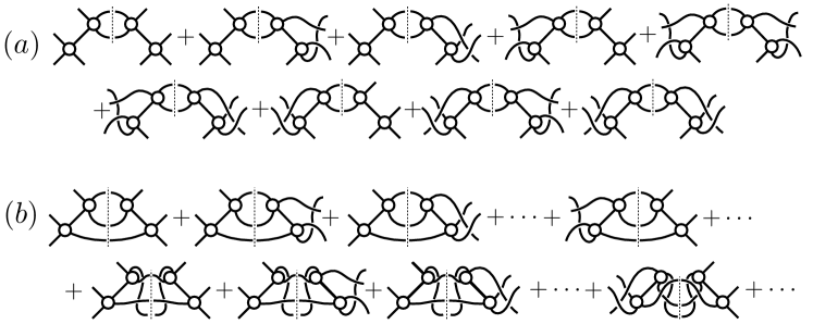
Figure 3: Counting of the $\bar{\rho}$ contributions in Eq. (56). (a) The nine contributions from the first term on the left-hand side of Eq. (56). The notation is as in Fig. 2, except that we do not display the external momenta, which are implicitly held fixed for all diagrams at the same values as in Fig. 2. Dashed lines depict the $\bar{\rho}$ cut, and the free ends in the middle of the diagram carry the momentum $\mathbf{s}$. (b) The $\bar{\rho}$-type contributions from the right-hand side of Eq. (56). Here the dashed line running through all three particles represents the integral on the right-hand side of Eq. (56). We do not show all 27 contributions; those not displayed are obtained by further permutations of the external lines, following the pattern shown in Fig. 2.

Finally, the last term in Eq. (48) gives the first contribution to the first term in Eq. (36). Specifically, we find

$$\mathcal{S}\left\{\int_{s}\mathcal{D}^{(1,u,u)^{*}}_{ps}[\Theta\bar{\rho}]_{s}\,\mathcal{D}^{(1,u,u)}_{sk}+\int_{s}\int_{t}\mathcal{D}^{(1,u,u)^{*}}_{ps}\Delta_{st}\mathcal{D}^{(1,u,u)}_{tk}\right\}=\\ \frac{1}{6}\frac{1}{2}\int_{p_{1}^{\prime\prime}}\int_{p_{2}^{\prime\prime}}\int_{p_{3}^{\prime\prime}}(2\pi)^{4}\delta^{4}(P-p_{1}^{\prime\prime}-p_{2}^{\prime\prime}-p_{3}^{\prime\prime})\ \mathcal{D}^{(1)*}(\mathbf{p}^{\prime};\mathbf{p}^{\prime\prime})\ \mathcal{D}^{(1)}(\mathbf{p}^{\prime\prime};\mathbf{p})\,.$$ (56)

Here the situation is similar to that in Eq. (50): The first term on the left-hand side is the symmetrization of the last term in Eq. (48), while the second term on the left-hand side comes from the next order term, i.e. ${\rm Im}\,\mathcal{D}^{(3)}$. Thus one needs only to show that the kinematic and counting factors from the first term on the left-hand side of Eq. (56) match those on the right-hand side coming from the contributions where the $\mathcal{M}_{2}$ factors in the two $\mathcal{D}^{(1)}$s match. This correspondence follows directly from

$$\int_{s}\Theta(E_{2,s}^{\star 2}-4m^{2})\bar{\rho}(\mathbf{s})\int_{\widehat{\mathbf{a}}^{\star}_{s}}\mathcal{F}(\textbf{s},\widehat{\mathbf{a}}^{\star}_{s})=\frac{1}{2}\frac{1}{2}\int_{p_{1}^{\prime\prime}}\int_{p_{2}^{\prime\prime}}\int_{p_{3}^{\prime\prime}}(2\pi)^{4}\delta^{4}(P-p_{1}^{\prime\prime}-p_{2}^{\prime\prime}-p_{3}^{\prime\prime})\mathcal{F}(\textbf{p}_{1}^{\prime\prime},\textbf{p}_{2}^{\prime\prime},\textbf{p}_{3}^{\prime\prime})\,,$$ (57)

where $\mathcal{F}$ is a test function. Thus we obtain an overall factor of $1/2$ instead of the required $1/6$. This is fixed by the relative counting factors. On the left-hand side there are 9 $\bar{\rho}$ terms, whereas on the right-hand side there are $(1/3)\times 9\times 9=27$, as shown in Fig. 3. The $1/3$ comes from the fact that when joining two $\mathcal{D}^{(1)}$s only one third of the terms have the $\bar{\rho}$ topology—the others matching with the $\Delta$ term on the left-hand side. In summary, the counting factors are 9 from the left-hand side and 27 from the right. These differ by exactly the left over $1/3$ remaining from the $1/6$.

III.2.3 Unitarity constraint on $\mathcal{D}^{(u,u)}$

We are now ready to argue that $\mathcal{M}^{(0)}=\mathcal{D}$ satisfies the unitarity relation to all orders. Starting directly from the integral equation, Eq. (38), and applying the key identity, Eq. (11), one finds

$${\rm Im}\mathcal{D}^{(u,u)}_{pk}=-\mathcal{M}_{2p}^{*}\,[\Theta\bar{\rho}]_{p}\,\mathcal{M}_{2p}\,G^{\infty}_{pk}\,\mathcal{M}_{2k}-\mathcal{M}_{2p}^{*}\,G^{\infty*}_{pk}\,\mathcal{M}^{*}_{2k}\,[\Theta\bar{\rho}]_{k}\,\mathcal{M}_{2k}+\mathcal{M}_{2p}^{*}\,\Delta_{pk}\,\mathcal{M}_{2k}\\ -\int_{s}\mathcal{M}_{2p}^{*}\,[\Theta\bar{\rho}]_{p}\,\mathcal{M}_{2p}\,G^{\infty}_{ps}\,\mathcal{D}^{(u,u)}_{sk}+\int_{s}\mathcal{M}_{2p}^{*}\,\Delta_{ps}\,\mathcal{D}^{(u,u)}_{sk}-\int_{s}\mathcal{M}_{2p}^{*}\,G^{\infty*}_{ps}\,{\rm Im}\mathcal{D}^{(u,u)}_{sk}\,.$$ (58)

Introducing shorthand for the delta function, $\tilde{\delta}_{pk}\equiv\tilde{\delta}(\mathbf{p}-\mathbf{k})$, this can be rewritten as

$$\int_{s}\left(\tilde{\delta}_{ps}+\mathcal{M}_{2p}^{*}G^{\infty*}_{ps}\right)\,{\rm Im}\mathcal{D}^{(u,u)}_{sk}=\mathcal{M}^{*}_{2p}\,[\Theta\bar{\rho}]_{p}\,\mathcal{D}^{(u,u)}_{pk}-\mathcal{M}_{2p}^{*}G^{\infty*}_{pk}\,\mathcal{M}^{*}_{2k}\,[\Theta\bar{\rho}]_{k}\,\mathcal{M}_{2k}\\ +\mathcal{M}_{2p}^{*}\,\Delta_{pk}\,\mathcal{M}_{2k}+\int_{s}\mathcal{M}_{2p}^{*}\,\Delta_{ps}\,\mathcal{D}^{(u,u)}_{sk}\,.$$ (59)

Figure 4: Diagrammatic representation of the right-hand side of Eq. (60), which gives the imaginary part of $\mathcal{D}^{{(u,u)}}$. Squares with rounded corners depict $\mathcal{D}^{{(u,u)}}$, and for simplicity we do not distinguish between $\mathcal{D}^{{(u,u)}}$ and its conjugate. The two types of cut, defined in the text, are distinguished by the shapes of the adjacent lines.

At this stage it is helpful to return to the result that we aim to prove, Eq. (36). Following the intuition developed in the analysis of $\mathcal{D}^{(1,u,u)}$ and $\mathcal{D}^{(2,u,u)}$, we note that $\mathcal{D}$ will satisfy the unitarity constraint if $\mathcal{D}^{(u,u)}$ satisfies

$${\rm Im}\,\mathcal{D}^{(u,u)}_{pk}=\mathcal{M}^{*}_{2p}\left([\Theta\bar{\rho}]_{p}\mathcal{D}^{(u,u)}_{pk}+\int_{s}\Delta_{ps}\mathcal{D}^{(u,u)}_{sk}\right)+\left(\mathcal{D}^{(u,u)*}_{pk}[\Theta\bar{\rho}]_{k}+\int_{s}\mathcal{D}^{(u,u)*}_{ps}\Delta_{sk}\right)\mathcal{M}_{2k}\\ +\mathcal{M}_{2p}^{*}\Delta_{pk}\mathcal{M}_{2k}+\left(\int_{s}\mathcal{D}^{(u,u)*}_{ps}[\Theta\bar{\rho}]_{s}\,\mathcal{D}^{(u,u)}_{sk}+\int_{s}\int_{t}\mathcal{D}^{(u,u)*}_{ps}\Delta_{st}\mathcal{D}^{(u,u)}_{tk}\right)\,.$$ (60)

This can be checked by applying $\mathcal{S}$ to both sides and taking advantage of the internal symmetrizations arising through $\Delta_{pk}$. We illustrate the right hand side of this equation in Fig. 4.

Thus our aim is to show that Eq. (59) implies Eq. (60). What we can easily show, instead, is the opposite implication, namely that Eq. (60) implies Eq. (59). To conclude that the results are in fact equivalent we require the additional assumption that the integral operator on the left-hand side of Eq. (59) is invertible. This is plausible since the operator is a deformation of the identity. Applying this operator to Eq. (60), one finds

$$\int_{s}\left(\tilde{\delta}_{ps}+\mathcal{M}_{2p}^{*}G^{\infty*}_{ps}\right){\rm Im}\,\mathcal{D}^{(u,u)}_{sk} =\int_{s}\left(\tilde{\delta}_{ps}+\mathcal{M}_{2p}^{*}G^{\infty*}_{ps}\right)\mathcal{M}^{*}_{2s}\left([\Theta\bar{\rho}]_{s}\mathcal{D}^{(u,u)}_{sk}+\int_{t}\Delta_{st}\mathcal{D}^{(u,u)}_{{t}k}\right)$$

$$+\int_{s}\left(\tilde{\delta}_{ps}+\mathcal{M}_{2p}^{*}G^{\infty*}_{ps}\right)\left(\mathcal{D}^{(u,u)*}_{sk}[\Theta\bar{\rho}]_{k}+\int_{t}\mathcal{D}^{(u,u)*}_{st}\Delta_{tk}\right)\mathcal{M}_{2k}$$

$$+\int_{s}\left(\tilde{\delta}_{ps}+\mathcal{M}_{2p}^{*}G^{\infty*}_{ps}\right)\mathcal{M}_{2s}^{*}\Delta_{sk}\mathcal{M}_{2k}$$

$$+\int_{s}\left(\tilde{\delta}_{ps}+\mathcal{M}_{2p}^{*}G^{\infty*}_{ps}\right)\left(\int_{t}\mathcal{D}^{(u,u)*}_{st}[\Theta\bar{\rho}]_{t}\mathcal{D}^{(u,u)}_{tk}+\int_{t}\int_{l}\mathcal{D}^{(u,u)*}_{st}\Delta_{tl}\mathcal{D}^{(u,u)}_{lk}\right)\,.$$ (61)

One can simplify this substantially using the integral equation defining $\mathcal{D}^{(u,u)}$, Eq. (14), which, after complex conjugation and rearrangement, leads to

$$\int_{s}\left(\tilde{\delta}_{ps}+\mathcal{M}_{2p}^{*}G^{\infty*}_{ps}\right)\mathcal{D}^{(u,u)*}_{sk}=-\mathcal{M}^{*}_{2p}G^{\infty*}_{pk}\mathcal{M}^{*}_{2k}\,.$$ (62)

After some straightforward algebra, one finds that the right hand side of Eq. (61) equals that of Eq. (59). Assuming the invertibility of the integral operator, as discussed above, it follows that the imaginary part of $\mathcal{D}^{(u,u)}$ satisfies Eq. (60), and consequently that $\mathcal{D}$ satisfies unitarity to all orders.

III.3 Unitarity of $\mathcal{M}_{3}$

Having shown in the previous section that the ${\mathcal{K}_{\mathrm{df},3}}$-independent part of $\mathcal{M}_{3}$ satisfies Eq. (36), in this section we show that this holds for the full three-body scattering amplitude. Following the approach of the previous section, we begin with the contribution that is linear in ${\mathcal{K}_{\mathrm{df},3}}$, denoted $\mathcal{M}_{3}^{(1)}$ and then generalize to the full amplitude.

As was the case with $\mathcal{D}^{(u,u)}$, it is instructive to first determine a constraint equation on $\mathcal{M}^{(1,u,u)}$ that is equivalent to the general unitarity constraint, Eq. (36)

$${\rm Im}\,\mathcal{M}^{(1,u,u)}_{3;pk}=\mathcal{M}^{*}_{2p}\left([\Theta\bar{\rho}]_{p}\,\mathcal{M}^{(1,u,u)}_{3;pk}+\int_{s}\Delta_{ks}\,\mathcal{M}^{(1,u,u)}_{3;sk}\,\right)+\left(\mathcal{M}^{(1,u,u)*}_{3;pk}\,[\Theta\bar{\rho}]_{k}+\int_{s}\mathcal{M}^{(1,u,u)*}_{3;ps}\,\Delta_{sk}\,\right)\mathcal{M}_{2k}\\ +\left(\int_{s}\mathcal{D}^{{{(u,u)}}*}_{ps}[\Theta\bar{\rho}]_{s}\mathcal{M}^{(1,u,u)}_{3;sk}+\int_{s}\int_{t}\mathcal{D}^{{{(u,u)}}*}_{ps}\Delta_{st}\mathcal{M}^{(1,u,u)}_{3;tk}\right)+\left(\int_{s}\mathcal{M}^{(1,u,u)*}_{ps}[\Theta\bar{\rho}]_{s}\mathcal{D}^{{{(u,u)}}}_{3;sk}+\int_{s}\int_{t}\mathcal{M}^{(1,u,u)*}_{ps}\,\Delta_{st}\,\mathcal{D}^{(u,u)}_{3;tk}\right)\,.$$ (63)

If the above is satisfied, $\mathcal{M}_{3}$ is consistent with unitarity through first order in ${\mathcal{K}_{\mathrm{df},3}}$. The relation is similar in structure to Eq. (60), except that the result here has more terms because the terms linear in ${\mathcal{K}_{\mathrm{df},3}}$ can occur both on the left and on the right of the imaginary cut. An analog of the third term in Eq. (60) is absent here because this term, which leads to the final term in Eq. (36), is already completely generated by $\mathcal{D}^{(u,u)}$. As with Eq. (60), the key point is that symmetrizing both sides gives the relevant contribution to the original unitarity constraint.

At this stage we note that our notation is overly complicated for two reasons: first, the same combination of $[\Theta\bar{\rho}]$ and $\Delta$ appears many times, and, second, all terms in this, and many of the preceding equations, have the form of a matrix product with common indices integrated. With this in mind we introduce the shorthand

$$\mathcal{I}_{ps}=[\Theta\bar{\rho}]_{p}\,\tilde{\delta}_{ps}+\Delta_{ps}\,,$$ (64)

and to adopt the convention that adjacent factors have a common index that is integrated over all values. We emphasize the latter convention by including a dot wherever there is a common, integrated index. With this notation, Eq. (63) reduces to

$${\rm Im}\,\mathcal{M}^{(1,u,u)}_{3}=(\mathcal{M}^{*}_{2}+\mathcal{D}^{{{(u,u)}}*})\cdot\mathcal{I}\cdot\mathcal{M}^{(1,u,u)}_{3}+\mathcal{M}^{(1,u,u)*}_{3}\cdot\mathcal{I}\cdot(\mathcal{M}_{2}+\mathcal{D}^{{{(u,u)}}})\,.$$ (65)

Note that we are implicitly multiplying $\mathcal{M}^{*}_{2}$ and $\mathcal{M}_{2}$ by a delta function in such expressions, for example

$$\left[\mathcal{M}^{*}_{2}\cdot\mathcal{I}\right]_{pr}\equiv\int_{t}\mathcal{M}^{*}_{2p}\tilde{\delta}_{pt}\mathcal{I}_{tr}=\mathcal{M}_{2p}^{*}\mathcal{I}_{pr}\,,$$ (66)

with no sum or integral in the final expression.

To show that the result is satisfied, we recall the definition of $\mathcal{M}_{3}^{(1,u,u)}$ given in Eqs. (30)-(32) above, which in our reduced notation becomes

$$\mathcal{M}_{3}^{(1,u,u)}=\mathcal{L}^{{(u,u)}}\cdot{\mathcal{K}_{\mathrm{df},3}}\cdot\mathcal{R}^{{(u,u)}}\,,$$ (67)

$$\mathcal{L}^{{(u,u)}}_{ps}=\tfrac{1}{3}\tilde{\delta}_{ps}-\mathcal{M}_{2p}\,\rho_{p}\,\tilde{\delta}_{ps}-\mathcal{D}^{{(u,u)}}_{ps}\,\rho_{s}\,,\qquad\mathcal{R}^{{(u,u)}}_{rk}=\tfrac{1}{3}\tilde{\delta}_{rk}-\rho_{k}\,\mathcal{M}_{2k}\,\tilde{\delta}_{rk}-\rho_{r}\,\mathcal{D}^{{(u,u)}}_{rk}\,.$$ (68)

We begin by taking the imaginary part of $\mathcal{L}^{{(u,u)}}_{ps}$

$${\rm Im}\,\mathcal{L}^{{(u,u)}}_{ps}=-\mathcal{M}_{2p}^{*}\,[\Theta\bar{\rho}]_{p}\,\mathcal{M}_{2p}\rho_{p}\tilde{\delta}_{ps}+\mathcal{M}_{2p}^{*}\,[\Theta\bar{\rho}]_{p}\,\tilde{\delta}_{ps}-{\rm Im}(\mathcal{D}^{{(u,u)}}_{ps})\rho_{s}+\mathcal{D}^{{{(u,u)}}*}_{ps}\,[\Theta\bar{\rho}]_{s}\,.$$ (69)

Substituting the result for ${\rm Im}\,\mathcal{D}^{{(u,u)}}_{ps}$ given by Eq. (60), we find

$$\begin{split}{\rm Im}\,\mathcal{L}^{{(u,u)}}_{ps}&=\mathcal{M}_{2p}^{*}\left\{[\Theta\bar{\rho}]_{p}\,\tilde{\delta}_{ps}-[\Theta\bar{\rho}]_{p}\tilde{\delta}_{ps}\,\mathcal{M}_{2s}\rho_{s}-\Delta_{ps}\mathcal{M}_{2s}\rho_{s}-[\Theta\bar{\rho}]_{p}\mathcal{D}^{(u,u)}_{ps}\rho_{s}-\int_{t}\Delta_{pt}\mathcal{D}^{(u,u)}_{ts}\rho_{s}\right\}\\ &\hskip 14.22636pt+\int_{t}\mathcal{D}^{{{(u,u)}}*}_{pt}\left\{[\Theta\bar{\rho}]_{t}\tilde{\delta}_{ts}-[\Theta\bar{\rho}]_{t}\tilde{\delta}_{ts}\mathcal{M}_{2s}\rho_{s}-\Delta_{ts}\mathcal{M}_{2s}\rho_{s}-[\Theta\bar{\rho}]_{t}\mathcal{D}^{{(u,u)}}_{ts}\rho_{s}-\int_{r}\Delta_{tr}\mathcal{D}^{{(u,u)}}_{rs}\rho_{s}\right\}\,,\end{split}$$ (70)

$$=\int_{t}\left(\mathcal{M}^{*}_{2p}\tilde{\delta}_{pt}+\mathcal{D}^{{{(u,u)}}*}_{pt}\right)\left\{[\Theta\bar{\rho}]_{t}\tilde{\delta}_{ts}-\int_{r}\mathcal{I}_{tr}\left(\mathcal{M}_{2r}\rho_{r}\tilde{\delta}_{rs}+\mathcal{D}^{{(u,u)}}_{rs}\rho_{s}\right)\right\}\,,$$ (71)

where in the second form we have collected terms by inserting delta-functions as needed and also by using the definition of $\mathcal{I}$, Eq. (64). Now we observe that the expression in curly braces in Eq. (71) would equal $\mathcal{I}\cdot\mathcal{L}^{(u,u)}$ were it not for the first term. However, we now make use of the replacement identity

$$[\Theta\bar{\rho}]_{p}\,\tilde{\delta}_{ps}\longrightarrow\frac{1}{3}\big{(}[\Theta\bar{\rho}]_{p}\,\tilde{\delta}_{ps}+\Delta_{ps}\big{)}=\frac{1}{3}\mathcal{I}_{ps}\,,\qquad{\text{(when\ acting\ on\ a\ symmetric\ object)}}\,.$$ (72)

This follows from the result Eq. (54), since for a symmetric object there is no difference between versions with $(u)$, $(s)$ and $(\tilde{s})$ superscripts. Note that the result applies irrespective of whether the action on a symmetric object is to the left or the right. Here the symmetric object on which $\mathcal{L}^{{(u,u)}}$ acts is ${\mathcal{K}_{\mathrm{df},3}}$ (to the right), as can be seen from Eq. (67).

Applying the identity (72) allows us to write Eq. (71) [and its reflection leading to ${\rm Im}\,\mathcal{R}^{{(u,u)}}$] in a compact form,

$${\rm Im}\,\mathcal{L}^{{(u,u)}} \longrightarrow\left(\mathcal{M}_{2}^{*}+\mathcal{D}^{{{(u,u)}}*}\right)\cdot\mathcal{I}\cdot\,\mathcal{L}^{{{(u,u)}}}\,,$$ (73)

$${\rm Im}\,\mathcal{R}^{{(u,u)}} \longrightarrow\mathcal{R}^{{{(u,u)}}*}\,\cdot\mathcal{I}\cdot\left(\mathcal{M}_{2}+\mathcal{D}^{{{(u,u)}}}\right)\,.$$ (74)

Since ${\mathcal{K}_{\mathrm{df},3}}$ is real, we have identified all contributions to ${\rm Im}\,\mathcal{M}^{(1,u,u)}_{3}$ [see Eq. (67)]. We deduce that

$${\rm Im}\,\mathcal{M}^{(1,u,u)}_{3} ={\rm Im}\big{(}\mathcal{L}^{{(u,u)}}\big{)}\cdot\mathcal{K}_{\mathrm{df},3}\cdot\mathcal{R}^{{(u,u)}}+\mathcal{L}^{{{(u,u)}}*}\cdot\mathcal{K}_{\mathrm{df},3}\cdot{\rm Im}\big{(}\mathcal{R}^{{(u,u)}}\big{)}\,,$$ (75)

$$=\left(\mathcal{M}^{*}_{2}+\mathcal{D}^{{{(u,u)}}*}\right)\cdot\mathcal{I}\cdot\mathcal{M}^{(1,u,u)}_{3}+\mathcal{M}^{(1,u,u)*}_{3}\cdot\mathcal{I}\cdot\left(\mathcal{M}_{2}+\mathcal{D}^{{(u,u)}}\right)\,,$$ (76)

which is indeed the desired result, Eq. (65).

Finally, we are in position to demonstrate that the complete connected three-body scattering amplitude, $\mathcal{M}_{3}=\mathcal{D}+\mathcal{M}_{3}^{(\mathcal{K})}$, satisfies the unitarity constraint, Eq. (36). This requires showing that $\mathcal{M}_{3}^{(\mathcal{K})}$ satisfies the parts of the constraint that depend on ${\mathcal{K}_{\mathrm{df},3}}$. As above, we rewrite these parts as a required constraint on the unsymmetrized version of $\mathcal{M}_{3}^{(\mathcal{K})}$,

$${\rm Im}\,\mathcal{M}^{(\mathcal{K},u,u)}_{3}=\left(\mathcal{M}^{*}_{2}+\mathcal{D}^{{{(u,u)}}*}\right)\cdot\mathcal{I}\cdot\mathcal{M}^{(\mathcal{K},u,u)}_{3}+\mathcal{M}^{(\mathcal{K},u,u)*}_{3}\cdot\mathcal{I}\cdot\left(\mathcal{M}_{2}+\mathcal{D}^{{(u,u)}}\right)+\ \mathcal{M}^{(\mathcal{K},u,u)*}_{3}\cdot\mathcal{I}\cdot\mathcal{M}^{(\mathcal{K},u,u)}_{3}\,.$$ (77)

Using the same steps as when considering Eqs. (63) and (65), we find that this symmetrizes to parts of Eq. (36) that depend on ${\mathcal{K}_{\mathrm{df},3}}$. Note that the last term of Eq. (36) does not need to be produced, as it is independent of ${\mathcal{K}_{\mathrm{df},3}}$, and has already been accounted for by ${\rm Im}\,\mathcal{D}$.

To demonstrate Eq. (77), we begin by giving the shorthand versions of the results, Eqs. (34) and (35), that give the ${\mathcal{K}_{\mathrm{df},3}}$-dependent part of $\mathcal{M}_{3}$,

$$\mathcal{M}^{(\mathcal{K},u,u)}_{3}=\mathcal{L}^{{(u,u)}}\cdot\mathcal{T}\cdot\mathcal{R}^{{(u,u)}}\,,\qquad\mathcal{T}=\mathcal{K}_{\mathrm{df},3}-\mathcal{K}_{\mathrm{df},3}\cdot\rho\mathcal{L}^{{(u,u)}}\cdot\mathcal{T}\,.$$ (78)

The imaginary part of $\mathcal{M}^{(\mathcal{K},u,u)}_{3}$,

$${\rm Im}\,\mathcal{M}^{(\mathcal{K},u,u)}_{3}={\rm Im}\big{(}\mathcal{L}^{{(u,u)}}\big{)}\cdot\mathcal{T}\cdot\mathcal{R}^{{(u,u)}}+\mathcal{L}^{{{(u,u)}}*}\cdot{\rm Im}\big{(}\mathcal{T}\big{)}\cdot\mathcal{R}^{{(u,u)}}+\mathcal{L}^{{{(u,u)}}*}\cdot\mathcal{T}\cdot{\rm Im}\big{(}\mathcal{R}^{{(u,u)}}\big{)}\,,$$ (79)

can be partially evaluated using the replacement rules Eqs. (73) and (74), which can be used since $\mathcal{T}$ is symmetric. This leads to

$${\rm Im}\,\mathcal{M}^{(\mathcal{K},u,u)}_{3}=\left(\mathcal{M}^{*}_{2}+\mathcal{D}^{{{(u,u)}}*}\right)\cdot\mathcal{I}\cdot\mathcal{M}^{(\mathcal{K},u,u)}_{3}+\mathcal{M}^{(\mathcal{K},u,u)*}_{3}\cdot\mathcal{I}\cdot\left(\mathcal{M}_{2}+\mathcal{D}^{{(u,u)}}\right)+\mathcal{L}^{{{(u,u)}}*}\cdot{\rm Im}\big{(}\mathcal{T}\big{)}\cdot\mathcal{R}^{{(u,u)}}\,.$$ (80)

Thus the first two terms in Eq. (77) are reproduced, and all that remains to demonstrate is

$$\mathcal{L}^{{{(u,u)}}*}\cdot{\rm Im}\left(\mathcal{T}\right)\cdot\mathcal{R}^{{(u,u)}}=\mathcal{M}^{(\mathcal{K},u,u)*}_{3}\cdot\mathcal{I}\cdot\mathcal{M}^{(\mathcal{K},u,u)}_{3}\,.$$ (81)

To do so requires evaluation of the imaginary part of $\mathcal{T}$. Using the integral equation in Eq.(78), the result (73) for the imaginary part of $\mathcal{L}^{{(u,u)}}$, and the reality of ${\mathcal{K}_{\mathrm{df},3}}$, we find

$${\rm Im}\,\mathcal{T}=\mathcal{K}_{\mathrm{df},3}\cdot[\Theta\bar{\rho}]\mathcal{L}^{{(u,u)}}\cdot\mathcal{T}-\mathcal{K}_{\mathrm{df},3}\cdot\rho^{*}(\mathcal{M}^{*}_{2}+\mathcal{D}^{{{(u,u)}}*})\cdot\mathcal{I}\cdot\mathcal{L}^{{(u,u)}}\cdot\mathcal{T}-\mathcal{K}_{\mathrm{df},3}\cdot\rho^{*}\mathcal{L}^{{{(u,u)}}*}\cdot{\rm Im}\,\mathcal{T}\,.$$ (82)

In the first term on the right-hand side one can apply the symmetrization identity (72) to write

$${\rm Im}\,\mathcal{T}=\mathcal{K}_{\mathrm{df},3}\cdot\mathcal{R}^{{{(u,u)}}*}\cdot\mathcal{I}\cdot\mathcal{L}^{{(u,u)}}\cdot\mathcal{T}-\mathcal{K}_{\mathrm{df},3}\cdot\rho^{*}\mathcal{L}^{{{(u,u)}}*}\cdot{\rm Im}\,\mathcal{T}\,,$$ (83)

where we have made use of the definition of $\mathcal{R}$, given in Eq. (68). The result (83) can be rewritten as

$$\mathcal{I}^{\mathcal{K}}\cdot{\rm Im}\,\mathcal{T} =\mathcal{K}_{\mathrm{df},3}\cdot\mathcal{R}^{{{(u,u)}}*}\cdot\mathcal{I}\cdot\mathcal{L}^{{(u,u)}}\cdot\mathcal{T}\,,$$ (84)

where we have introduced

$$\mathcal{I}^{\mathcal{K}}_{pr}\equiv\tilde{\delta}_{pr}+\int_{s}\mathcal{K}_{\mathrm{df},3;ps}\rho_{s}^{*}\mathcal{L}^{{{(u,u)}}*}_{sr}\,,$$ (85)

which acts as an integral operator.

We now observe that this same operator can be used to rewrite the complex conjugate of the relation between ${\mathcal{K}_{\mathrm{df},3}}$ and $\mathcal{T}$ given in Eq. (78),

$$\mathcal{K}_{\mathrm{df},3}=\mathcal{I}^{\mathcal{K}}\cdot\mathcal{T}^{*}\,.$$ (86)

Thus we find

$${\mathcal{I}}^{\mathcal{K}}\cdot{\rm Im}\,\mathcal{T}={\mathcal{I}}^{\mathcal{K}}\cdot\mathcal{T}^{*}\cdot\mathcal{R}^{{{(u,u)}}*}\cdot\mathcal{I}\cdot\mathcal{L}^{{(u,u)}}\cdot\mathcal{T}\,.$$ (87)

Assuming that ${\mathcal{I}}^{\mathcal{K}}$ is invertible, which is plausible using the same arguments given in Sec. III.2.3 for the integral operator encountered previously, we can drop the factors of this operator to reach

$${\rm Im}\,\mathcal{T}=\mathcal{T}^{*}\cdot\mathcal{R}^{{{(u,u)}}*}\cdot\mathcal{I}\cdot\mathcal{L}^{{(u,u)}}\cdot\mathcal{T}\,.$$ (88)

Finally, inserting this result into the left-hind side of Eq. (81), we immediately find the right-hand side, concluding the argument.

IV Conclusion

In this work we have shown that the form of the infinite-volume three-particle scattering amplitude, $\mathcal{M}_{3}$, derived in the context of finite-volume formalism, satisfies unitarity. Though this result was expected, the demonstration turns out to be highly nontrivial, and thus provides an important check of the derivations of Refs. Hansen and Sharpe (2014, 2015). In particular, the present derivation shows how the factors of $1/3$ in the expressions for $\mathcal{L}^{{(u,u)}}$ and $\mathcal{R}^{{(u,u)}}$ given in Eq. (68) are essential for unitarity to hold. Such factors are not present in the alternative representations of Refs. Mai et al. (2017); Jackura et al. (2018), and were initially a source of confusion in understanding the consistency of the various approaches.

More generally, we have shown how ${\mathcal{K}_{\mathrm{df},3}}$ and ${\cal D}$ individually contribute to the imaginary part of the connected amplitude. While the latter is a somewhat standard object representing all-orders resummation of the one-particle exchange interactions, ${\mathcal{K}_{\mathrm{df},3}}$ is a quantity unique to the formalism of Refs. Hansen and Sharpe (2014, 2015). It was introduced in Ref. Hansen and Sharpe (2014) as a fully symmetric amplitude that encodes the short-distance or microscopic physics. In analogy to the two-particle K matrix it has no unitary branch cuts and is real for real energies.

In other approaches, e.g. Refs. Mai et al. (2017); Jackura et al. (2018), similar objects appear, but these are not invariant under particle interchange. The work presented here can shed light on the connection between these formalisms, as well as to other approaches that derive three-body amplitudes from unitarity relations Amado (1975); Aaron and Amado (1973); Aitchison and Pasquier (1966); Cook and Lee (1962); Ball et al. (1962); Fleming (1964); Holman (1965). Indeed, the relation between ${\mathcal{K}_{\mathrm{df},3}}$ and the $B$-matrix used in Refs. Mai et al. (2017); Jackura et al. (2018) has been determined in Ref. Jackura et al. . We also think that it will be worthwhile investigating the use of the ${\mathcal{K}_{\mathrm{df},3}}$-parametrization of $\mathcal{M}_{3}$ in analyses of experimental data. Given that the finite-volume observables that may be accessed via lattice QCD are more directly related to ${\mathcal{K}_{\mathrm{df},3}}$ Hansen and Sharpe (2014), this will serve as a stepping stone towards bridging three-body physics in experiment and lattice QCD.

V Acknowledgements

This work was supported by U.S. Department of Energy contracts DE-SC0011637 (SRS), DE-FG02-87ER40365 (APS), and DE-AC05-06OR23177 (RAB, APS) under which Jefferson Science Associates, LLC, manages and operates Jefferson Lab, and National Science Foundation under Grant No. PHY-1415459 (APS). RAB also acknowledges support from the U.S. Department of Energy Early Career award, contract DE-SC0019229. SRS also acknowledges partial supported from the International Research Unit of Advanced Future Studies at Kyoto University.

Appendix A Unitarity relation for the three-body scattering amplitude

In this appendix we review the derivation of Eq. (36), the constraint that follows from unitarity on the three-particle scattering amplitude.

Unitarity implies that the $T$ matrix satisfies $T-T^{\dagger}=iT^{\dagger}T$. To derive the resulting constraint we evaluate matrix elements of this equation using relativistically-normalized three-particle asymptotic states, $|\textbf{p}\rangle=|\textbf{p}_{1},\textbf{p}_{2},\textbf{p}_{3}\rangle$. This yields

$$\langle\textbf{p}^{\prime}|T|\textbf{p}\rangle-\langle\textbf{p}^{\prime}|T^{\dagger}|\textbf{p}\rangle =2i{\rm Im}\,\langle\textbf{p}^{\prime}|T|\textbf{p}\rangle=\frac{i}{3!}\iiint_{p^{\prime\prime}}\langle\textbf{p}^{\prime}|T^{\dagger}|\textbf{p}^{\prime\prime}\rangle\,\langle\textbf{p}^{\prime\prime}|T|\textbf{p}\rangle=\frac{i}{3!}\iiint_{p^{\prime\prime}}\langle\textbf{p}^{\prime}|T|\textbf{p}^{\prime\prime}\rangle^{*}\,\langle\textbf{p}^{\prime\prime}|T|\textbf{p}\rangle\,,$$ (89)

where we have used

$$\langle\textbf{p}^{\prime}|T^{\dagger}|\textbf{p}\rangle\equiv\langle\textbf{p}|T|\textbf{p}^{\prime}\rangle^{*}=\langle\textbf{p}^{\prime}|T|\textbf{p}\rangle^{*}\,,$$ (90)

in which the second equality follows from hermitian analyticity Eden et al. (1966); Olive (1962), as well as the shorthand notation

$$\iiint_{p}=\int_{p_{1}}\int_{p_{2}}\int_{p_{3}}\,.$$ (91)

The factor of $3!$ in the denominator is needed for identical particles to cancel the overcounting arising from integrating over the full three-particle phase space. The result (89) can be rewritten as

$${\rm Im}\,\langle\textbf{p}^{\prime}|T|\textbf{p}\rangle=\frac{1}{2\,\times 3!}\int_{p^{\prime}}\langle\textbf{p}^{\prime}|T|\textbf{p}^{\prime\prime}\rangle^{*}\,\langle\textbf{p}^{\prime\prime}|T|\textbf{p}\rangle\,.$$ (92)

In the following, we also need the total initial and final four-momenta

$$P^{\mu} =(E,\mathbf{P})=(\omega_{p_{1}}+\omega_{p_{2}}+\omega_{p_{3}},\mathbf{p}_{1}+\mathbf{p}_{2}+\mathbf{p}_{3})\,,$$ (93)

$$P^{\prime\prime\mu} =(E^{\prime\prime},\mathbf{P}^{\prime\prime})=(\omega_{p^{\prime\prime}_{1}}+\omega_{p^{\prime\prime}_{2}}+\omega_{p^{\prime\prime}_{3}},\mathbf{p}^{\prime\prime}_{1}+\mathbf{p}^{\prime\prime}_{2}+\mathbf{p}^{\prime\prime}_{3})\,.$$ (94)

Next we decompose the T matrix into disconnected and connected pieces,

$$T=T_{\text{d}}+T_{\text{c}}\,,$$ (95)

with the disconnected piece having the matrix element

$$\langle\textbf{p}^{\prime\prime}|T_{\text{d}}|\textbf{p}\rangle =\sum_{j,k}\tilde{\delta}(\textbf{p}^{\prime\prime}_{j}-\textbf{p}_{k})(2\pi)^{4}\delta^{4}(P^{\prime\prime}_{j}-P_{k})\mathcal{A}_{2,jk}(\textbf{p}^{\prime\prime};\textbf{p})\,,$$ (96)

$$=(2\pi)^{4}\delta^{4}(P^{\prime\prime}-P)\sum_{j,k}\tilde{\delta}(\textbf{p}^{\prime\prime}_{j}-\textbf{p}_{k})\mathcal{A}_{2,jk}(\textbf{p}^{\prime\prime};\textbf{p})\,,$$ (97)

where the indices $j$ and $k$ run from 1 to 3. Here $\mathcal{A}_{2,jk}(\textbf{p}^{\prime\prime};\textbf{p})$ is the two-particle scattering amplitude for the subsystem defined by the fact that the initial and final spectators have momentua $\mathbf{p}_{k}$ and $\mathbf{p}^{\prime\prime}_{j}$, respectively, while $P^{\prime\prime}_{j}=P-p^{\prime\prime}_{j}=(E-\omega_{p^{\prime\prime}_{j}},\textbf{P}-\textbf{p}^{\prime\prime}_{j})$ and $P_{k}=P-p_{k}$. The corresponding result for the connected part is

$$\langle\textbf{p}^{\prime\prime}|T_{\text{c}}|\textbf{p}\rangle=(2\pi)^{4}\delta^{4}(P^{\prime}-P)\mathcal{A}_{3}(\textbf{p}^{\prime};\textbf{p})\,,$$ (98)

where $\mathcal{A}_{3}$ is the connected three-particle amplitude.

To proceed we insert the decomposition (95) into the unitarity relation, Eq. (92). The left-hand side becomes

$${\rm LHS} =[{\rm LHS}]_{c}+[{\rm LHS}]_{d}\,,$$ (99)

$$[{\rm LHS}]_{c} =(2\pi)^{4}\delta^{4}(P^{\prime}-P)\,{\rm Im}\,\mathcal{A}_{3}(\textbf{p}^{\prime};\textbf{p})\,,$$ (100)

$$[{\rm LHS}]_{d} =(2\pi)^{4}\delta^{4}(P^{\prime}-P)\sum_{j,k}\tilde{\delta}(\textbf{p}^{\prime}_{j}-\textbf{p}_{k}){\rm Im}\,\mathcal{A}_{2,jk}(\textbf{p}^{\prime};\textbf{p})\,,$$ (101)

while for the right-hand side we obtain

$${\rm RHS}=\frac{1}{2\,\times 3!}\iiint_{p^{\prime\prime}}\bigg{\{}\langle\textbf{p}^{\prime}|T_{\text{c}}|\textbf{p}^{\prime\prime}\rangle^{*}\,\langle\textbf{p}^{\prime\prime}|T_{\text{c}}|\textbf{p}\rangle+\langle\textbf{p}^{\prime}|T_{\text{c}}|\textbf{p}^{\prime\prime}\rangle^{*}\,\langle\textbf{p}^{\prime\prime}|T_{\text{d}}|\textbf{p}\rangle\\ +\langle\textbf{p}^{\prime}|T_{\text{d}}|\textbf{p}^{\prime\prime}\rangle^{*}\,\langle\textbf{p}^{\prime\prime}|T_{\text{c}}|\textbf{p}\rangle+\langle\textbf{p}^{\prime}|T_{\text{d}}|\textbf{p}^{\prime\prime}\rangle^{*}\,\langle\textbf{p}^{\prime\prime}|T_{\text{d}}|\textbf{p}\rangle\bigg{\}}\,.$$ (102)

Our aim is to determine the parts of this expression that equal $[{\rm LHS}]_{c}$, for these give the unitarity relation for $\mathcal{A}_{3}$.

We label the four terms in Eq. (102) as $[{\rm RHS}]_{1-4}$. The first three are fully connected, while the last contains disconnected contributions. To pull out the latter we insert the expression for the disconnected contribution to the T matrix, Eq. (97), into the final term in Eq. (102), obtaining

$$[{\rm RHS}]_{4} =\frac{1}{2\,\times 3!}\sum_{j,k,\ell,n}\iiint_{p^{\prime\prime}}\tilde{\delta}(\textbf{p}^{\prime}_{j}-\textbf{p}^{\prime\prime}_{\ell})\tilde{\delta}(\textbf{p}^{\prime\prime}_{n}-\textbf{p}_{k})(2\pi)^{4}\delta^{4}(P^{\prime}-P^{\prime\prime})(2\pi)^{4}\delta^{4}(P^{\prime\prime}-P)\mathcal{A}^{*}_{2,{j\ell}}(\textbf{p}^{\prime};\textbf{p}^{\prime\prime})\mathcal{A}_{2,nk}(\textbf{p}^{\prime\prime};\textbf{p}).$$ (103)

Here we are using $j$ and $k$ for the external spectator indices, and $\ell$ and $n$ for the internal indices. There are two types of contribution to Eq. (103): those in which $\ell=n$, which are fully disconnected since the same momentum is a spectator for both scatterings, and the connected contributions in which $\ell\neq n$. For a given choice of $j$ and $k$, there are 3 contributions of the first kind and 6 of the second. We denote the fully disconnected contributions by $[{\rm RHS}]_{4d}$, and the connected by $[{\rm RHS}]_{4c}$.

The three contributions to the fully disconnected part are all equal when considering identical particles, so we can set $\ell=n=j$ and multiply by an overall factor of three. This allows us to write

$$[{\rm RHS}]_{4d} =\frac{(2\pi)^{4}\delta^{4}(P^{\prime}-P)}{2\,\times 2}\sum_{j,k}\iiint_{p^{\prime\prime}}\tilde{\delta}(\textbf{p}^{\prime}_{j}-\textbf{p}_{k})\tilde{\delta}(\textbf{p}^{\prime\prime}_{j}-\textbf{p}_{k})(2\pi)^{4}\delta^{4}(P^{\prime\prime}-P)\mathcal{A}^{*}_{2,{jj}}(\textbf{p}^{\prime};\textbf{p}^{\prime\prime})\mathcal{A}_{2,jk}(\textbf{p}^{\prime\prime};\textbf{p})\,.$$ (104)

Next we use the result Eq. (57), which, after carrying out the remaining spectator-momentum integral, gives

$$[{\rm RHS}]_{4{\text{d}}} ={(2\pi)^{4}\delta^{4}(P^{\prime}-P)}\sum_{j,k}\Theta(E_{2,p_{k}}^{*\,2}-4m^{2})\bar{\rho}(\mathbf{p}_{k})\tilde{\delta}(\textbf{p}^{\prime}_{j}-\textbf{p}_{k})\int\frac{d\widehat{\mathbf{a}}^{\star}_{p^{\prime\prime}_{j}}}{4\pi}\mathcal{A}^{*}_{2,jj}(\textbf{p}^{\prime};\textbf{p}^{\prime\prime})\mathcal{A}_{2,jk}(\textbf{p}^{\prime\prime};\textbf{p})\,.$$ (105)

We recall that $\widehat{\mathbf{a}}^{\star}_{p^{\prime\prime}_{j}}$ is the direction of one of the intermediate particles in the center of mass of the two-particle subsystem for which $\mathbf{p}^{\prime\prime}_{j}$ is the spectator momentum.

Equating the fully disconnected contributions to the left- and right-hand sides of the unitarity relation, which are given respectively by Eqs. (101) and (105), we find

$${\rm Im}\,\mathcal{A}_{2,jk}(\textbf{p}^{\prime};\textbf{p}) =\Theta(E_{2,p_{k}}^{*\,2}-4m^{2})\bar{\rho}(\mathbf{p}_{k})\int\frac{d\widehat{\mathbf{a}}^{\star}_{p^{\prime\prime}_{j}}}{4\pi}\mathcal{A}^{*}_{2,jj}(\textbf{p}^{\prime};\textbf{p}^{\prime\prime})\mathcal{A}_{2,jk}(\textbf{p}^{\prime\prime};\textbf{p})\,.$$ (106)

This is the standard unitarity constraint on the two-body scattering amplitude, as given, for example, in Eqs. (6) and (7) of Ref. Jackura et al. (2018), taking into account that here we have an additional factor of $1/2$ on the right-hand side due to our use of identical particles.

We now evaluate the connected piece of Eq. (103),

$$[{\rm RHS}]_{4\text{c}} =\frac{(2\pi)^{4}\delta^{4}(P^{\prime}-P)}{2\,\times 3!}\sum_{j,k,\ell\neq n}\iiint_{p^{\prime\prime}}\tilde{\delta}(\textbf{p}^{\prime}_{j}-\textbf{p}^{\prime\prime}_{\ell})\tilde{\delta}(\textbf{p}^{\prime\prime}_{n}-\textbf{p}_{k})(2\pi)^{4}\delta^{4}(P^{\prime\prime}-P)\mathcal{A}^{*}_{2,{j\ell}}(\textbf{p}^{\prime};\textbf{p}^{\prime\prime})\mathcal{A}_{2,nk}(\textbf{p}^{\prime\prime};\textbf{p})\,,$$ (107)

$$=\frac{(2\pi)^{4}\delta^{4}(P^{\prime}-P)}{2}\sum_{j,k}\iiint_{p^{\prime\prime}}\tilde{\delta}(\textbf{p}^{\prime}_{j}-\textbf{p}^{\prime\prime}_{\bar{k}})\tilde{\delta}(\textbf{p}^{\prime\prime}_{\bar{\jmath}}-\textbf{p}_{k})(2\pi)^{4}\delta^{4}(P^{\prime\prime}-P)\mathcal{A}^{*}_{2,{j1}}(\textbf{p}^{\prime};\textbf{p}^{\prime\prime})\mathcal{A}_{2,3k}(\textbf{p}^{\prime\prime};\textbf{p})\,,$$ (108)

$$={(2\pi)^{4}\delta^{4}(P^{\prime}-P)}\sum_{j,k}\pi\,\delta(b_{jk}^{2}-m^{2})\,\mathcal{A}^{*}_{2,{j1}}(\textbf{p}^{\prime};\textbf{p}^{\prime\prime})\mathcal{A}_{2,3k}(\textbf{p}^{\prime\prime};\textbf{p})\,.$$ (109)

To obtain the second line we have used the fact that all six terms in the sum over $\ell\neq n$ are equal, since they differ only by the choice of dummy indices. We have thus made a canonical choice ($\ell=1$ and $n=3$) and multiplied by six. To obtain the final line we have simply carried out the integrals, and used the definition $b_{jk}\equiv P-p^{\prime}_{j}-p_{k}$.

The remaining terms in Eq. (102) are more straightforward to evaluate. For example, the second term gives

$${\rm[RHS]_{2}} =\frac{1}{2\,\times 3!}\sum_{jk}\iiint_{p^{\prime\prime}}\langle\textbf{p}^{\prime}|T_{\text{c}}|\textbf{p}^{\prime\prime}\rangle^{*}\,\tilde{\delta}(\textbf{p}^{\prime\prime}_{j}-\textbf{p}_{k})(2\pi)^{4}\delta^{4}(P^{\prime\prime}-P)\mathcal{A}_{2,jk}(\textbf{p}^{\prime\prime};\textbf{p})\,,$$ (110)

$$=\frac{(2\pi)^{4}\delta^{4}(P^{\prime}-P)}{2\,\times 3!}\sum_{jk}\iiint_{p^{\prime\prime}}\mathcal{A}^{*}_{3}(\textbf{p}^{\prime};\textbf{p}^{\prime\prime})\,\tilde{\delta}(\textbf{p}^{\prime\prime}_{j}-\textbf{p}_{k})(2\pi)^{4}\delta^{4}(P^{\prime\prime}-P)\mathcal{A}_{2,jk}(\textbf{p}^{\prime\prime};\textbf{p})\,,$$ (111)

$$={(2\pi)^{4}\delta^{4}(P^{\prime}-P)}\sum_{j}\Theta(E_{2,p_{j}}^{*\,2}-4m^{2})\bar{\rho}(\mathbf{p}_{j})\int\frac{d\widehat{\mathbf{a}}^{\prime\prime\star}_{p_{j}}}{4\pi}\mathcal{A}^{*}_{3}(\textbf{p}^{\prime};\textbf{p}^{\prime\prime})\,\mathcal{A}_{2,jj}(\textbf{p}^{\prime\prime};\textbf{p})\,.$$ (112)

In going from the second to third line, we have again used Eq. (57), and the fact that we are summing over three values of $k$, all of which give the same contribution.

The third term in Eq. (102) can be written similarly (interchanging $\mathbf{p}\leftrightarrow\mathbf{p}^{\prime}$ and complex conjugating), while the first term becomes

$${\rm[RHS]_{1}}=\frac{(2\pi)^{4}\delta^{4}(P^{\prime}-P)}{2\times 3!}\iiint_{p^{\prime\prime}}{(2\pi)^{4}\delta^{4}(P^{\prime\prime}-P)}\mathcal{A}^{*}_{3}(\mathbf{p}^{\prime};\mathbf{p}^{\prime\prime})\mathcal{A}_{3}(\mathbf{p}^{\prime\prime};\mathbf{p})\,.$$ (113)

Equating $[{\rm LHS}]_{c}$ to ${\rm[RHS]_{1}}+{\rm[RHS]_{2}}+{\rm[RHS]_{3}}+{\rm[RHS]_{4c}}$ leads to the claimed unitarity relation, Eq. (36).

References

• Hansen and Sharpe (2015) M. T. Hansen and S. R. Sharpe, Phys. Rev. D92, 114509 (2015), eprint 1504.04248.
• Bjorken (1960) J. D. Bjorken, Phys. Rev. Lett. 4, 473 (1960).
• Aitchison and Pasquier (1966) I. J. R. Aitchison and R. Pasquier, Phys. Rev. 152, 1274 (1966).
• Ascoli and Wyld (1975) G. Ascoli and H. W. Wyld, Phys. Rev. D12, 43 (1975).
• Magalhaes et al. (2011) P. C. Magalhaes, M. R. Robilotta, K. S. F. F. Guimaraes, T. Frederico, W. de Paula, I. Bediaga, A. C. d. Reis, C. M. Maekawa, and G. R. S. Zarnauskas, Phys. Rev. D84, 094001 (2011), eprint 1105.5120.
• Mai et al. (2017) M. Mai, B. Hu, M. Döring, A. Pilloni, and A. Szczepaniak, Eur. Phys. J. A53, 177 (2017), eprint 1706.06118.
• Mikhasenko et al. (2019) M. Mikhasenko, Y. Wunderlich, A. Jackura, V. Mathieu, A. Pilloni, B. Ketzer, and A. P. Szczepaniak (2019), eprint 1904.11894.
• Jackura et al. (2018) A. Jackura, C. Fernández-Ramírez, V. Mathieu, M. Mikhasenko, J. Nys, A. Pilloni, K. Saldana, N. Sherrill, and A. P. Szczepaniak (2018), eprint 1809.10523.
• Lüscher (1986) M. Lüscher, Commun.Math.Phys. 105, 153 (1986).
• Lüscher (1991) M. Lüscher, Nucl.Phys. B354, 531 (1991).
• Rummukainen and Gottlieb (1995) K. Rummukainen and S. A. Gottlieb, Nucl. Phys. B450, 397 (1995), eprint hep-lat/9503028.
• Kim et al. (2005) C. h. Kim, C. T. Sachrajda, and S. R. Sharpe, Nucl. Phys. B727, 218 (2005), eprint hep-lat/0507006.
• He et al. (2005) S. He, X. Feng, and C. Liu, JHEP 07, 011 (2005), eprint hep-lat/0504019.
• Lage et al. (2009) M. Lage, U.-G. Meißner, and A. Rusetsky, Phys.Lett. B681, 439 (2009), eprint 0905.0069.
• Fu (2012) Z. Fu, Phys.Rev. D85, 014506 (2012), eprint 1110.0319.
• Hansen and Sharpe (2012) M. T. Hansen and S. R. Sharpe, Phys.Rev. D86, 016007 (2012), eprint 1204.0826.
• Briceño and Davoudi (2013a) R. A. Briceño and Z. Davoudi, Phys. Rev. D88, 094507 (2013a), eprint 1204.1110.
• Göckeler et al. (2012) M. Göckeler, R. Horsley, M. Lage, U.-G. Meißner, P. E. L. Rakow, A. Rusetsky, G. Schierholz, and J. M. Zanotti, Phys. Rev. D86, 094513 (2012), eprint 1206.4141.
• Briceño (2014) R. A. Briceño, Phys. Rev. D89, 074507 (2014), eprint 1401.3312.
• Lellouch and Lüscher (2001) L. Lellouch and M. Lüscher, Commun.Math.Phys. 219, 31 (2001), eprint hep-lat/0003023.
• Christ et al. (2005) N. H. Christ, C. Kim, and T. Yamazaki, Phys.Rev. D72, 114506 (2005), eprint hep-lat/0507009.
• Meyer (2011) H. B. Meyer, Phys. Rev. Lett. 107, 072002 (2011), eprint 1105.1892.
• Bernard et al. (2012) V. Bernard, D. Hoja, U. G. Meißner, and A. Rusetsky, JHEP 09, 023 (2012), eprint 1205.4642.
• Agadjanov et al. (2014) A. Agadjanov, V. Bernard, U. G. Meißner, and A. Rusetsky, Nucl. Phys. B886, 1199 (2014), eprint 1405.3476.
• Briceño et al. (2015) R. A. Briceño, M. T. Hansen, and A. Walker-Loud, Phys. Rev. D91, 034501 (2015), eprint 1406.5965.
• Feng et al. (2015) X. Feng, S. Aoki, S. Hashimoto, and T. Kaneko, Phys. Rev. D91, 054504 (2015), eprint 1412.6319.
• Briceño and Hansen (2015) R. A. Briceño and M. T. Hansen, Phys. Rev. D92, 074509 (2015), eprint 1502.04314.
• Briceño and Hansen (2016) R. A. Briceño and M. T. Hansen, Phys. Rev. D94, 013008 (2016), eprint 1509.08507.
• Baroni et al. (2018) A. Baroni, R. A. Briceño, M. T. Hansen, and F. G. Ortega-Gama (2018), eprint 1812.10504.
• Wilson et al. (2015) D. J. Wilson, R. A. Briceño, J. J. Dudek, R. G. Edwards, and C. E. Thomas, Phys. Rev. D92, 094502 (2015), eprint 1507.02599.
• Briceño et al. (2017) R. A. Briceño, J. J. Dudek, R. G. Edwards, and D. J. Wilson, Phys. Rev. Lett. 118, 022002 (2017), eprint 1607.05900.
• Brett et al. (2018) R. Brett, J. Bulava, J. Fallica, A. Hanlon, B. Hörz, and C. Morningstar, Nucl. Phys. B932, 29 (2018), eprint 1802.03100.
• Guo et al. (2018) D. Guo, A. Alexandru, R. Molina, M. Mai, and M. Döring, Phys. Rev. D98, 014507 (2018), eprint 1803.02897.
• Andersen et al. (2018) C. W. Andersen, J. Bulava, B. Hörz, and C. Morningstar, Phys. Rev. D97, 014506 (2018), eprint 1710.01557.
• Andersen et al. (2019) C. Andersen, J. Bulava, B. Hörz, and C. Morningstar, Nucl. Phys. B939, 145 (2019), eprint 1808.05007.
• Dudek et al. (2014) J. J. Dudek, R. G. Edwards, C. E. Thomas, and D. J. Wilson (Hadron Spectrum), Phys. Rev. Lett. 113, 182001 (2014), eprint 1406.4158.
• Dudek et al. (2016) J. J. Dudek, R. G. Edwards, and D. J. Wilson (Hadron Spectrum), Phys. Rev. D93, 094506 (2016), eprint 1602.05122.
• Woss et al. (2018) A. Woss, C. E. Thomas, J. J. Dudek, R. G. Edwards, and D. J. Wilson, JHEP 07, 043 (2018), eprint 1802.05580.
• Woss et al. (2019) A. J. Woss, C. E. Thomas, J. J. Dudek, R. G. Edwards, and D. J. Wilson (2019), eprint 1904.04136.
• Briceño et al. (2018a) R. A. Briceño, J. J. Dudek, and R. D. Young, Rev. Mod. Phys. 90, 025001 (2018a), eprint 1706.06223.
• Beane et al. (2013) S. R. Beane, E. Chang, S. D. Cohen, W. Detmold, H. W. Lin, T. C. Luu, K. Orginos, A. Parreno, M. J. Savage, and A. Walker-Loud (NPLQCD), Phys. Rev. D87, 034506 (2013), eprint 1206.5219.
• Cheung et al. (2017) G. K. C. Cheung, C. E. Thomas, J. J. Dudek, and R. G. Edwards (Hadron Spectrum), JHEP 11, 033 (2017), eprint 1709.01417.
• Detmold and Nicholson (2013) W. Detmold and A. N. Nicholson, Phys. Rev. D88, 074501 (2013), eprint 1308.5186.
• Hörz and Hanlon (2019) B. Hörz and A. Hanlon (2019), eprint 1905.04277.
• Polejaeva and Rusetsky (2012) K. Polejaeva and A. Rusetsky, Eur.Phys.J. A48, 67 (2012), eprint 1203.1241.
• Briceño and Davoudi (2013b) R. A. Briceño and Z. Davoudi, Phys. Rev. D87, 094507 (2013b), eprint 1212.3398.
• Hansen and Sharpe (2014) M. T. Hansen and S. R. Sharpe, Phys. Rev. D90, 116003 (2014), eprint 1408.5933.
• Hammer et al. (2017a) H.-W. Hammer, J.-Y. Pang, and A. Rusetsky, JHEP 09, 109 (2017a), eprint 1706.07700.
• Hammer et al. (2017b) H. W. Hammer, J. Y. Pang, and A. Rusetsky, JHEP 10, 115 (2017b), eprint 1707.02176.
• Guo and Gasparian (2017) P. Guo and V. Gasparian, Phys. Lett. B774, 441 (2017), eprint 1701.00438.
• Mai and Döring (2017) M. Mai and M. Döring, Eur. Phys. J. A53, 240 (2017), eprint 1709.08222.
• Briceño et al. (2017) R. A. Briceño, M. T. Hansen, and S. R. Sharpe, Phys. Rev. D95, 074510 (2017), eprint 1701.07465.
• Döring et al. (2018) M. Döring, H. W. Hammer, M. Mai, J. Y. Pang, A. Rusetsky, and J. Wu, Phys. Rev. D97, 114508 (2018), eprint 1802.03362.
• Briceño et al. (2018b) R. A. Briceño, M. T. Hansen, and S. R. Sharpe, Phys. Rev. D98, 014506 (2018b), eprint 1803.04169.
• Mai and Döring (2019) M. Mai and M. Döring, Phys. Rev. Lett. 122, 062503 (2019), eprint 1807.04746.
• Briceño et al. (2019) R. A. Briceño, M. T. Hansen, and S. R. Sharpe, Phys. Rev. D99, 014516 (2019), eprint 1810.01429.
• Blanton et al. (2019) T. D. Blanton, F. Romero-López, and S. R. Sharpe, JHEP 03, 106 (2019), eprint 1901.07095.
• Hansen and Sharpe (2019) M. T. Hansen and S. R. Sharpe (2019), eprint 1901.00483.
• Bedaque et al. (1999a) P. F. Bedaque, H. W. Hammer, and U. van Kolck, Phys. Rev. Lett. 82, 463 (1999a), eprint nucl-th/9809025.
• Bedaque et al. (1999b) P. F. Bedaque, H. W. Hammer, and U. van Kolck, Nucl. Phys. A646, 444 (1999b), eprint nucl-th/9811046.
• Aaron and Amado (1973) R. Aaron and R. D. Amado, Phys. Rev. Lett. 31, 1157 (1973).
• Amado (1974) R. D. Amado, Phys. Rev. Lett. 33, 333 (1974).
• Fleming (1964) G. N. Fleming, Phys. Rev. 135, B551 (1964).
• Amado (1975) R. D. Amado, Phys. Rev. C12, 1354 (1975).
• Cook and Lee (1962) L. F. Cook and B. W. Lee, Phys. Rev. 127, 283 (1962).
• Ball et al. (1962) J. S. Ball, W. Frazer, and M. Nauenberg, Phys. Rev. 128, 478 (1962).
• Holman (1965) W. J. Holman, III, Phys. Rev. 138, B1286 (1965).
• (68) W. Jackura, S. Dawid, C. Fernández-Ramírez, V. Mathieu, M. Mikhasenko, A. Pilloni, S. Sharpe, and A. Szczepaniak, work in progress.
• Eden et al. (1966) R. J. Eden, P. V. Landshoff, D. I. Olive, and J. C. Polkinghorne, The Analytic S-Matrix (Cambridge University Press, Cambridge, 1966).
• Olive (1962) D. I. Olive, Nuovo Cim. 26, 73 (1962).