Autonomous Interpretation of Demonstrations for Modification of Dynamical Movement Primitives

Abstract

The concept of dynamical movement primitives (DMPs) has become popular for modeling of motion, commonly applied to robots. This paper presents a framework that allows a robot operator to adjust DMPs in an intuitive way. Given a generated trajectory with a faulty last part, the operator can use lead-through programming to demonstrate a corrective trajectory. A modified DMP is formed, based on the first part of the faulty trajectory and the last part of the corrective one. A real-time application is presented and verified experimentally.

I Introduction

High cost for time-consuming robot programming, performed by engineers, has become a key obstruction in industrial manufacturing. This has promoted the research towards faster and more intuitive means of robot programming, such as learning from demonstration, of which an introduction is presented in [1]. It is in this context desirable to make robot teaching available to a broader group of practitioners by minimizing the engineering work required during teaching of tasks.

A costumary way to quickly mediate tasks to robots is to use lead-through programming, while saving trajectory data so that the robot can reproduce the motion. In this paper, the data are used to form dynamical movement primitives (DMPs). Early versions of these were presented in [2], [3] and [4], and put into context in [5]. Uncomplicated modification for varying tasks was emphasized in this literature. For example, the time scale was governed by one parameter, which could be adjusted to fit the purpose. Further, the desired final state could be adjusted, to represent a motion similar to the original one but to a different goal. DMPs applied on object handover with moving targets were addressed in [6]. The scalability in space was demonstrated in, e.g., [7].

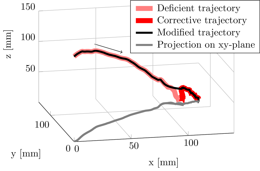
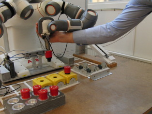
The scenario considered in this paper is the unfavorable event that the last part of the motion generated by a certain DMP is unsatisfactory. There might be several reasons for this to occur. In the case where the starting points differ, the generated trajectory would still converge to the demonstrated end point, but take a modified path, where the modification would be larger for larger differences between the starting points. Further, the DMP might have been created in a slightly different setup, e.g., for a different robot or robot cell. There might also have been a mistake in the teaching that the operator would have to undo. If the whole last part of the trajectory is of interest, it is not enough to modify the goal state only. One way to solve the problem would be to record an entirely new trajectory, and then construct a corresponding DMP. However, this would be unnecessarily time consuming for the operator, as only the last part of the trajectory has to be modified. Instead, the method described here allows the operator to lead the manipulator backwards, approximately along the part of the trajectory that should be adjusted, followed by a desired trajectory, as visualized in Fig. 2.

Figure 1: The ABB YuMi prototype robot used in the experiments.

Figure 2: Trajectories of the robot’s end-effector from one of the experiments. The arrow indicates the direction. The deficient trajectory was generated from the original DMP. After that, the operator demonstrated the corrective trajectory. Merging of these, resulted in the modified trajectory. The projection on the xy-plane is only to facilitate the visualization.

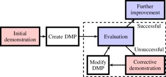
Hitherto, DMPs have usually been formed by demonstrations to get close to the desired behavior, followed by trajectory-based reinforcement learning, as presented in, e.g., [8, 9, 10, 11]. Compared to such refinements, the modification presented here is less time consuming and does not require engineering work. On the other hand, the previous work on reinforcement learning offers modulation based on sensor data, and finer movement adjustment. Therefore, the framework presented in this paper forms an intermediate step, where, if necessary, a DMP is modified to prepare for reinforcement learning, see Fig. 5. This modification can be used within a wide range of tasks. In this paper, we exemplify by focusing on peg-in-hole tasks.

In [8], online modulation, such as obstacle avoidance, was implemented for DMPs. This approach has been verified for several realistic scenarios, but requires an infrastructure for obstacle detection, as well as some coupling term parameters to be defined. It preserves convergence to the goal point, but since the path to get there is modified by the obstacle avoidance, it is not guaranteed to follow any specific trajectory to the goal. This is significant for, e.g., a peg-in-hole task.

The paper is outlined as follows. Two example scenarios in which the framework would be useful are presented in Sec. III, followed by a description of the method in Sec. IV. Experimental setup and results are described in Sections V and VI, and finally a discussion and concluding remarks are presented in Sections VII and VIII, respectively.

II Problem Formulation

In this paper, we address the question whether it is possible to automatically interpret a correction, made by an operator, of the last part of a DMP trajectory, while still taking advantage of the first part. The human-robot interaction must be intuitive, and the result of a correction predictable enough for its purpose. The correction should result in a new DMP, of which the first part behaves qualitatively as the first part of the original DMP, whereas the last part resembles the last part of the corrective trajectory. Any discontinuity between the original and corrective trajectories must be mitigated.

III Motivating Examples

We here describe two scenarios where the framework proves useful. These are evaluated in Sections V and VI, where more details are given.

III-A Inadequate precision - Scenario A

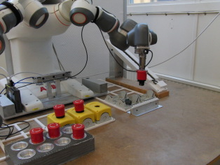
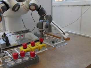
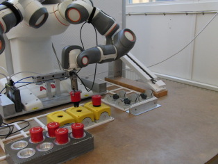
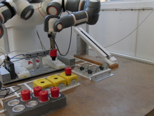
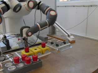
Consider the setup shown in Fig. 3, where the button should be placed into the yellow case. A DMP was run for this purpose, but, due to any of the reasons described above, the movement was not precise enough, and the robot got stuck on its way to the target, see Fig. 3(b). Hitherto, such a severe shortcoming would have motivated the operator to teach a completely new DMP, and erase the old one. With the method proposed here, the operator had the opportunity to approve the first part of the trajectory, and only had to modify the last part. This was done by leading the robot arm backwards, approximately along the faulty path, until it reached the acceptable part. Then, the operator continued to lead the arm along a desired path to the goal. When this was done, the acceptable part of the first trajectory was merged with the last part of the corrective trajectory. After that, a DMP was fitted to the resulting trajectory. Compared to just updating the target point, this approach also allowed the operator to determine the trajectory leading there. This scenario is referred to as Scenario A.

(a)

(b)

(c)

(d)

Figure 3: Scenario A. The evaluation started in (a), and in (b) the robot failed to place the button in the hole due to inadequate accuracy. Between (a) and (b), the deficient trajectory was recorded. The operator led the robot arm (c) backwards, approximately along a proportion of the deficient trajectory, and subsequently led it to place the button properly, while the corrective trajectory was recorded. The robot then made the entire motion, starting in a configuration similar to that in (a), and ending as displayed in (d).

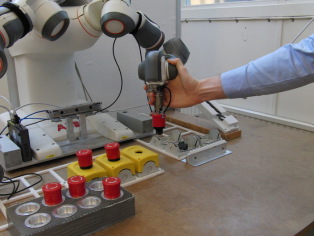
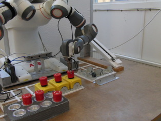
III-B New obstacle - Scenario B

For the setup in Fig. 4, there existed a DMP for moving the robot arm from the right, above the button that was already inserted, to a position just above the hole in the leftmost yellow case. However, under the evaluation the operator realized that there would have been a collision if a button were already placed in the case in the middle. A likely reason for this to happen would be that the DMP was created in a slightly different scene, where the potential obstacle was not taken into account. Further, the operator desired to extend the movement to complete the peg-in-hole task, rather than stopping above the hole. With the method described herein, the action of the operator would be similar to that described in Sec. III-A, again saving work compared to previous methods. This scenario is referred to as Scenario B.

(a)

(b)

(c)

(d)

(e)

(f)

Figure 4: Scenario B. The initial goal was to move the button to the leftmost yellow case, above the hole, to prepare for placement. The evaluation started in (a), and in (b) the trajectory was satisfactory as the placed button was avoided. In (c), however, there would have been a collision if there was a button placed in the middle case. Further, it was desired to complete the peg-in-hole task, rather than stopping above the hole. Hence, the evaluated trajectory was considered deficient. In (d), the operator led the robot arm back, and then in a motion above the potential obstacle, and into the hole, forming the corrective trajectory. Based on the modified DMP, the robot started in a position similar to that in (a), avoided the potential obstacle in (e) and reached the new target in (f). The trajectories from one attempt are shown in Fig. 10.

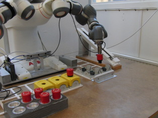
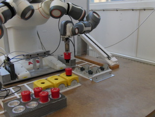
IV Description of the Framework

In this section, the concept of DMPs is first introduced. A method to determine what parts of the deficient and corrective trajectories to retain is presented, followed by a description of how these should be merged to avoid discontinuities. Finally, some implementation aspects are addressed. Figure 5 displays a schematic overview of the work flow of the application, from the user’s perspective.

Figure 5: Schematic visualization of the work flow, from an operator’s perspective. A DMP was created based on a demonstration. Subsequently, the DMP was executed while evaluated by the operator. If unsuccessful, the operator demonstrated a correction, which yielded a modified DMP to be evaluated. Once successful, further improvement could be done by, e.g., trajectory-based reinforcement learning, though that was outside the scope of this work. Steps that required direct, continuous interaction by the operator are marked with light red color. Steps that required some attention, such as supervision and initialization, are marked with light blue. The operations in the white boxes were done by the software in negligible computation time, and required no human involvement. The work in this paper focused on the steps within the dashed rectangle.

IV-A Dynamical movement primitives

A review of the DMP concept was presented in [7], and here follows a short description of how it was applied in this context. A certain trajectory, $y$, was modeled by the system

$$\tau\dot{y}=z,$$ (1)

where $z$ is determined by

$$\tau\dot{z}= \alpha_{z}(\beta_{z}(g-y)-z)+f(x)$$ (2)

In turn, $f(x)$ is a function given by

$$f(x)= \frac{\sum_{i=1}^{N_{b}}\Psi_{i}(x)w_{i}}{\sum_{i=1}^{N_{b}}\Psi_{i}(x)}x\cdot(g-y_{0}),$$ (3)

where the basis functions, $\Psi_{i}(x)$, take the form

$$\Psi_{i}(x)= \exp\left(-\frac{1}{2\sigma_{i}^{2}}(x-c_{i})^{2}\right)$$ (4)

$$\tau\dot{x}= -\alpha_{x}x$$ (5)

Here, $\tau$ is a time constant, while $\alpha_{z}$, $\beta_{z}$ and $\alpha_{x}$ are positive parameters. Further, $N_{b}$ is the number of basis functions, $w_{i}$ is the weight for basis function $i$, $y_{0}$ is the starting point of the trajectory $y$, and $g$ is the goal state. $\sigma_{i}$ and $c_{i}$ are the standard deviation and mean of each basis function, respectively. Given a DMP, a robot trajectory can be generated from Eqs. 1 and 2. Vice versa, given a demonstrated trajectory, $y_{demo}$, a corresponding DMP can be formed; $g$ is then given by the end position of $y_{demo}$, whereas $\tau$ can be set to get a desired time scale. Further, the solution of a weighted linear regression problem in the sampled domain yields the weights

$$w_{i}=\frac{\boldsymbol{s}^{T}\boldsymbol{\Gamma}_{i}\boldsymbol{f}_{target}}{\boldsymbol{s}^{T}\boldsymbol{\Gamma}_{i}\boldsymbol{s}},\text{where}\hskip 5.69054pt\boldsymbol{s}=\begin{pmatrix}x^{1}(g-y_{demo}^{1})\\ x^{2}(g-y_{demo}^{1})\\ \vdots\\ x^{N}(g-y_{demo}^{1})\end{pmatrix},$$ (6)

$$\boldsymbol{\Gamma_{i}}=\text{diag}(\Psi_{i}^{1},\Psi_{i}^{2}\cdots\Psi_{i}^{N}),\hskip 5.69054pt\boldsymbol{f}_{target}=\begin{pmatrix}f_{target}^{1}\\ f_{target}^{2}\\ \vdots\\ f_{target}^{N}\end{pmatrix},$$ (7)

$$f_{target}=\tau^{2}\ddot{y}_{demo}-a_{z}(b_{z}(g-y_{demo})-\tau\dot{y}_{demo}).$$ (8)

Here, $N$ is the number of samples in the demonstrated trajectory.

IV-B Interpretation of corrective demonstration

If the evaluation of a trajectory was unsuccessful, a corrective demonstration and DMP modification should follow (Fig. 5). Denote by $y_{d}$ the deficient trajectory, and by $y_{c}$ the corrective one, of which examples are shown in Figs. 2, 6 and 7. A trajectory formed by simply appending $y_{c}$ to $y_{d}$ was likely to take an unnecessary detour. Thus, only the first part of $y_{d}$ and the last part of $y_{c}$ were retained. This is illustrated in Fig. 7. Denote by $y_{cr}$ the retained part of the corrective trajectory. The operator signaled where to separate the corrective trajectory, during the corrective demonstration. In the current implementation, this was done by pressing a button in a terminal user interface, when the robot configuration corresponded to the desired starting point of $y_{cr}$, denoted $y_{cr}^{1}$.

Figure 6: Visualization of shortest distance, here denoted $d_{m}$, used to determine the left separation marker in Fig. 7. The trajectories are the same as in Figs. 2 and 7, except that the modified trajectory is omitted.

Figure 7: Same trajectories as in Fig. 2, but zoomed in on the corrective trajectory. Arrows indicate directions. The parts of the trajectories between the separation markers were not retained. The right, blue, separation point was determined explicitly by the operator during the corrective demonstration. The left, green, separation point was determined according to Eq. 10. Further, what was left of the deficient trajectory was modified for a smooth transition. However, the part of the corrective trajectory retained was not modified, since it was desired to closely follow this part of the demonstration. Note that the trajectories retained were not intended for direct play-back execution. Instead, they were used to form a modified DMP, which in turn generated a resulting trajectory, as shown in Figs. 8, 9 and 10.

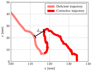
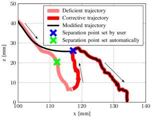
The next step was to determine which part of $y_{d}$ to retain. This was chosen as the part previous to the sample on $y_{d}$ that was closest to $y_{cr}^{1}$, i.e.,

$$y_{dr}^{m}=y_{d}^{m},\hskip 11.38109pt\forall m\in[1;M]$$ (9)

where

$$M=\operatornamewithlimits{argmin}\limits_{k=1\dots K}\operatorname{d}(y_{d}^{k},y_{cr}^{1})$$ (10)

Here, $\operatorname{d}$ denotes distance, and $K$ is the number of samples in $y_{d}$, see Fig. 6 for an illustration. The approach of using the shortest distance as a criteria, was motivated by the assumption that the operator led the robot arm back, approximately along the deficient trajectory, until the part that was satisfactory. At this point, the operator separated the corrective demonstration, thus defining $y_{cr}^{1}$ (see right marker in Fig. 7). By removing parts of the demonstrated trajectories, a significant discontinuity between the remaining parts was introduced. In order to counteract this, $y_{dr}$ was modified into $y_{m}$, where the following features were desired.

• $y_{m}$ should follow $y_{dr}$ approximately

• The curvature of $y_{m}$ should be moderate

• $y_{m}$ should end where $y_{cr}$ began, with the same direction in this point

To find a suitable trade-off between these objectives, the following convex optimization problem was solved:

$$\underset{y_{m}}{\text{minimize}} \lVert y_{dr}-y_{m}\rVert_{2}+\lambda\lVert T_{(\Delta^{2})}y_{m}\rVert_{2}$$ (11)

subject to $$y_{m}^{M}=y_{cr}^{1}$$ (12)

$$y_{m}^{M}-y_{m}^{M-1}=y_{cr}^{2}-y_{cr}^{1}$$ (13)

Here, $\lambda$ denotes a constant scalar, and $T_{(\Delta^{2})}$ is a second-order finite difference operator. Subsequently, $y_{cr}$ was appended on $y_{m}$, and one corresponding DMP was created, with the method described in the previous subsection. The next step in the work flow was to evaluate the resulting DMP (Fig. 5).

IV-C Software implementation

The research interface ExtCtrl [12], [13], was used to send references to the low-level robot joint controller in the ABB IRC5 system [14], at 250 Hz. Most of the programming was done in C++, where DMPs were stored as objects. Among the data members of this class were the parameters $\tau$, $g$ and $w_{1\dots N_{b}}$, as well as some description of the context of the DMP and when it was created. It contained member functions for displaying the parameters, and for modifying $g$ and $\tau$. The communication between the C++ program and ExtCtrl was handled by the LabComm protocol [15]. The C++ linear algebra library Armadillo [16] was used in a major part of the implementation. Further, the code generator CVXGEN [17] was used to generate C code for solving the optimization problem in Eqs. (11), (12) and (13). By default, the solver code was optimized with respect to computation time. This resulted in a real-time application, in which the computation times were negligible in teaching scenarios. The optimization problem was typically solved well below one millisecond on an ordinary PC.

V Experiments

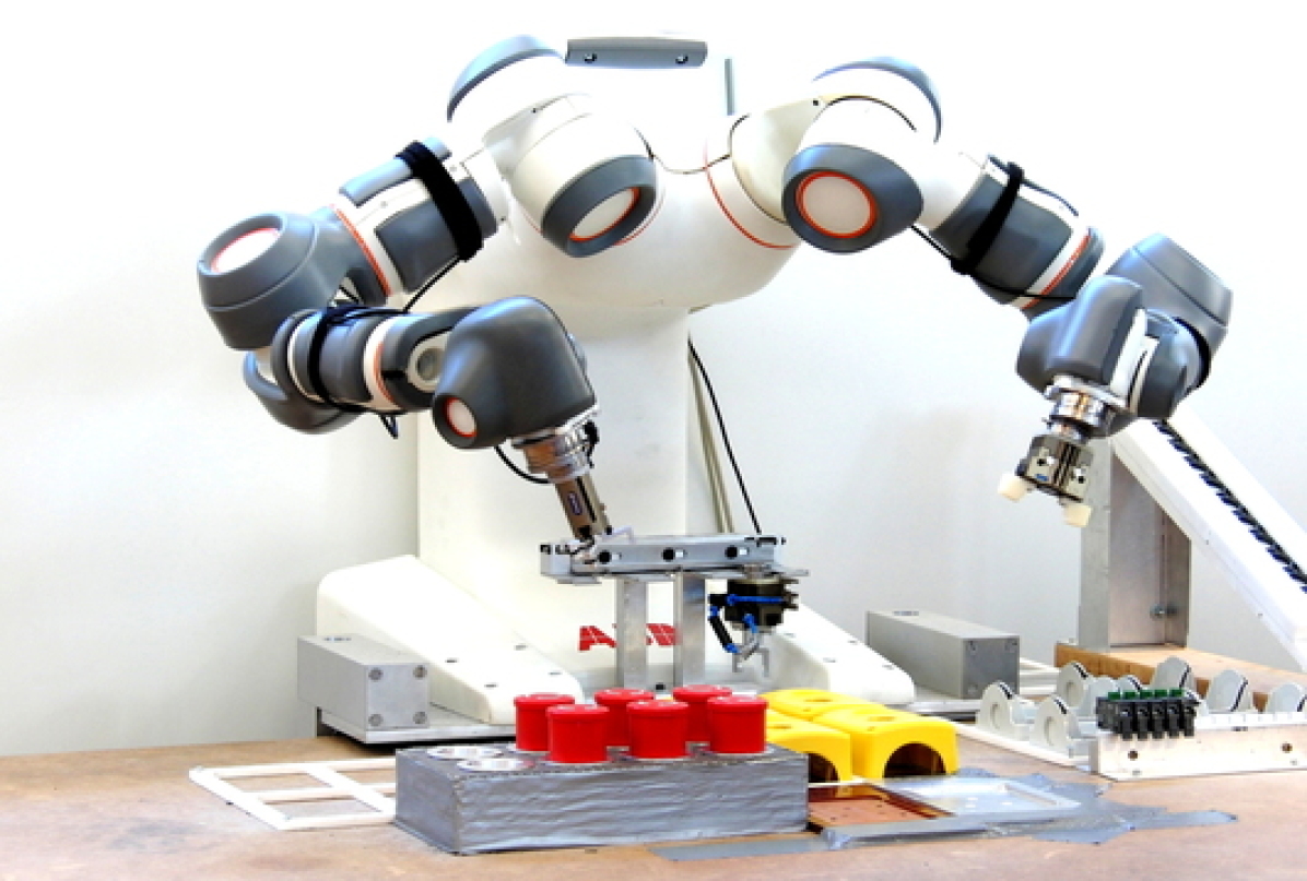
The robot used in the experimental setup was a prototype of the dual-arm ABB YuMi [18] (previously under the name FRIDA) robot, with 7 joints per arm, see Fig. 1. The experiments were performed in real-time using the implementation described in Sec. IV-C. The computations took place in joint space, and the robot’s forward kinematics was used for visualization in Cartesian space in the figures presented. The scenarios in Sec. III were used to evaluate the proposed method. For each trial, the following steps were taken.

• An initial trajectory was taught, deliberately failing to meet the requirements, as explained in Sec. III.

• Based on this, a DMP was created.

• The DMP was used to generate a trajectory similar to the initial one. This formed the deficient trajectory.

• A corrective trajectory was recorded.

• Based on the correction, a resulting DMP was formed automatically.

• The resulting DMP was executed for experimental evaluation.

First, Scenario A was set up for evaluation, see Sec. III-A and Fig. 3. The scenario started with execution of a deficient trajectory. For each attempt, a new deficient trajectory was created and modified. A total of 50 attempts were made.

Similarly, Scenario B (see Sec. III-B and Fig. 4) was set up, and again, a total of 50 attempts were made.

A video is available as a publication attachment, to facilitate understanding of the experimental setup and results. A version with higher resolution is available on [19].

VI Results

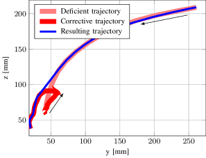
For each attempt of Scenario A, the robot was able to place the button properly in the yellow case after modification. Results from two of these attempts are shown in Figs. 8 and 9. In the first case, the deficient trajectory went past the goal, whereas in the second case, it did not reach far enough.

Figure 8: Trajectories from the experimental evaluation of Scenario A. The deficient trajectory went past the goal in the negative $y$-direction, preventing the robot from lowering the button into the hole. After correction, the robot was able to reach the target as the modified DMP generated the resulting trajectory.

Figure 9: Similar to Fig. 8, except that in this case, the deficient trajectory did not reach far enough in the negative $y$-direction.

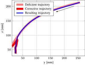
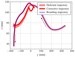
Each of the attempts of Scenario B were also successful. After modification, the DMPs generated trajectories that moved the grasped stop button above the height of potential obstacles, in this case other stop buttons, and subsequently inserted it into the case. The result from one attempt is shown in Fig. 10.

Figure 10: Trajectories from experimental evaluation of Scenario B. The deficient trajectory was lowered too early, causing a potential collision. After the correction, the robot was able to reach the target while avoiding the obstacles. The movement was also extended to perform the entire peg-in-hole task, rather than stopping above the hole.

VII Discussion

The subsequent step in this work is to integrate the presented framework with trajectory-based reinforcement learning [8], [20], in order to optimize the motion locally with respect to criteria such as execution time. The program should also be augmented to take the purpose of, and relation between, different DMPs into consideration. This extension will emphasize the necessity of keeping track of different states within the work flow. To this purpose, a state machine implemented in, e.g., JGrafchart [21], or the framework of behavior trees, applied on robot control in [22], would be suitable. Extending the user interface with support for natural language, would possibly make this framework more user friendly.

Performing the computations in joint space instead of Cartesian space allowed the operator to determine the entire configuration of the 7 DOF robot arm, rather than the pose of the tool only. However, one could think of situations where the operator is not concerned by the configuration, and the pose of the tool would be more intuitive to consider. It would therefore be valuable if it could be determined whether the operator aimed to adjust the configuration or just the pose of the tool. For example, a large configuration change yielding a small movement of the tool, should promote the hypothesis that the operator aimed to adjust the configuration.

It should be stated that the scenarios evaluated here are not covering the whole range of plausible scenarios related to this method, and it remains as future work to investigate the generalizability, and user experience, more thoroughly. The last part of the resulting movement is guaranteed to follow the retained part of the corrective demonstration accurately, given enough DMP basis functions. Hence, the only source of error on that part is a faulty demonstration. For instance, the movement might require higher accuracy than what is possible to demonstrate using lead-through programming. Another limitation with this method is that it is difficult for the operator to very accurately determine which part of the faulty trajectory to retain, since this is done autonomously. However, for the experiments performed here, the estimation of the operator was sufficient to demonstrate desired behavior. The benefit with this approach is that it saves time as the operator does not have to specify all details explicitly.

VIII Conclusions

In this paper, an approach for modification of DMPs, using lead-through programming, was presented. It allowed a robot operator to modify the last part of a faulty generated trajectory, instead of demonstrating a new one from the beginning. Based on the corrective demonstration, modified DMPs were formed automatically. A real-time application, that did not require any additional engineering work by the user, was developed, and verified experimentally. A video showing the functionality is available as a publication attachment, and a version with higher resolution is available on [19].

References

- [1] B. D. Argall, S. Chernova, M. Veloso, and B. Browning, “A survey of robot learning from demonstration,” Robotics and Autonomous Systems, vol. 57, no. 5, pp. 469–483, 2009.
- [2] A. J. Ijspeert, J. Nakanishi, and S. Schaal, “Movement imitation with nonlinear dynamical systems in humanoid robots,” in IEEE International Conference on Robotics and Automation (ICRA), Proceedings, vol. 2. Washington D.C.: IEEE, May 11-15 2002, pp. 1398–1403.
- [3] S. Schaal, A. Ijspeert, and A. Billard, “Computational approaches to motor learning by imitation,” Philosophical Transactions of the Royal Society of London B: Biological Sciences, vol. 358, no. 1431, pp. 537–547, 2003.
- [4] A. Ijspeert, J. Nakanishi, and S. Schaal, “Learning control policies for movement imitation and movement recognition,” in Neural Information Processing System, vol. 15, 2003, pp. 1547–1554.
- [5] S. Niekum, S. Osentoski, G. Konidaris, S. Chitta, B. Marthi, and A. G. Barto, “Learning grounded finite-state representations from unstructured demonstrations,” The International Journal of Robotics Research, vol. 34, no. 2, pp. 131–157, 2015.
- [6] M. Prada, A. Remazeilles, A. Koene, and S. Endo, “Implementation and experimental validation of dynamic movement primitives for object handover,” in IEEE/RSJ International Conference on Intelligent Robots and Systems (IROS). Chicago, Illinois: IEEE, Sept. 14–18 2014, pp. 2146–2153.
- [7] A. J. Ijspeert, J. Nakanishi, H. Hoffmann, P. Pastor, and S. Schaal, “Dynamical movement primitives: learning attractor models for motor behaviors,” Neural Computation, vol. 25, no. 2, pp. 328–373, 2013.
- [8] P. Pastor, M. Kalakrishnan, F. Meier, F. Stulp, J. Buchli, E. Theodorou, and S. Schaal, “From dynamic movement primitives to associative skill memories,” Robotics and Autonomous Systems, vol. 61, no. 4, pp. 351–361, 2013.
- [9] J. Kober, B. Mohler, and J. Peters, “Learning perceptual coupling for motor primitives,” in 2008 IEEE/RSJ International Conference on Intelligent Robots and Systems. Nice, France: IEEE, Sep 22-26 2008, pp. 834–839.
- [10] F. J. Abu-Dakka, B. Nemec, J. A. Jørgensen, T. R. Savarimuthu, N. Krüger, and A. Ude, “Adaptation of manipulation skills in physical contact with the environment to reference force profiles,” Autonomous Robots, vol. 39, no. 2, pp. 199–217, 2015.
- [11] P. J. Kroemer O, Detry R and P. J, “Combining active learning and reactive control for robot grasping,” Robotics and Autonomous Systems (RAS), vol. 58, no. 9, p. 1105–1116, 2010.
- [12] A. Blomdell, G. Bolmsjö, T. Brogårdh, P. Cederberg, M. Isaksson, R. Johansson, M. Haage, K. Nilsson, M. Olsson, T. Olsson, A. Robertsson, and J. Wang, “Extending an industrial robot controller-implementation and applications of a fast open sensor interface,” IEEE Robotics & Automation Magazine, vol. 12, no. 3, pp. 85–94, 2005.
- [13] A. Blomdell, I. Dressler, K. Nilsson, and A. Robertsson, “Flexible application development and high-performance motion control based on external sensing and reconfiguration of abb industrial robot controllers,” in IEEE International Conference on Robotics and Automation (ICRA), Anchorage, Alaska, May 3-8 2010, pp. 62–66.
- [14] ABB Robotics. (2017) ABB IRC5. Accessed: 2017-01-23. [Online]. Available: http://new.abb.com/products/robotics/controllers/irc5
- [15] Dept. Automatic Control, Lund University. (2017) Research tools and software. Accessed: 2017-02-13. [Online]. Available: http://www.control.lth.se/Research/tools.html
- [16] C. Sanderson, “Armadillo: An open source C++ linear algebra library for fast prototyping and computationally intensive experiments,” 2010.
- [17] J. Mattingley and S. Boyd, “CVXGEN: A code generator for embedded convex optimization,” Optimization and Engineering, vol. 13, no. 1, pp. 1–27, 2012.
- [18] ABB Robotics. (2017) ABB YuMi. Accessed: 2017-01-23. [Online]. Available: http://new.abb.com/products/robotics/yumi
- [19] M. Karlsson. (2017) Modification of dynamical movement primitives, Youtube. Accessed: 2017-01-25. [Online]. Available: https://www.youtube.com/watch?v=q998JUwofX4&feature=youtu.be
- [20] F. Stulp, J. Buchli, A. Ellmer, M. Mistry, E. A. Theodorou, and S. Schaal, “Model-free reinforcement learning of impedance control in stochastic environments,” IEEE Transactions on Autonomous Mental Development, vol. 4, no. 4, pp. 330–341, 2012.
- [21] A. Theorin, “A sequential control language for industrial automation,” Ph.D. dissertation, TFRT–1104–SE, Dept. Automatic Control, Lund University, Lund, Sweden, 2014.
- [22] A. Marzinotto, M. Colledanchise, C. Smith, and P. Ogren, “Towards a unified behavior trees framework for robot control,” in IEEE International Conference on Robotics and Automation (ICRA). Hong Kong, China: IEEE, May 31-June 7 2014, pp. 5420–5427.