Disentangling Dynamics and Returns: Value Function Decomposition with Future Prediction

Abstract

Value functions are crucial for model-free Reinforcement Learning (RL) to obtain a policy implicitly or guide the policy updates. Value estimation heavily depends on the stochasticity of environmental dynamics and the quality of reward signals. In this paper, we propose a two-step understanding of value estimation from the perspective of future prediction, through decomposing the value function into a reward-independent future dynamics part and a policy-independent trajectory return part. We then derive a practical deep RL algorithm from the above decomposition, consisting of a convolutional trajectory representation model, a conditional variational dynamics model to predict the expected representation of future trajectory and a convex trajectory return model that maps a trajectory representation to its return. Our algorithm is evaluated in MuJoCo continuous control tasks and shows superior results under both common settings and delayed reward settings.

1 Introduction

Reinforcement learning (RL) is one promising approach to obtain the optimal policy in sequential decision-making problems based on reward signals during interaction with the environment. Most popular RL algorithms are model-free since they do not need the access to the environment models. Value functions play an important role in model-free RL [27], which are usually used to derive a policy implicitly in value-based methods [18] or guide the policy updates in policy-based methods [21, 25]. With deep neural networks, value functions can be well-estimated even with large state and action space, making it practical for model-free RL to deal with more challenging tasks [16, 18, 24].

Value functions define the expected cumulative rewards of a policy, indicating the degree a state or an action could be beneficial. They are usually estimated through Monte Carlo (MC) or Temporal Difference (TD) algorithms [27], without explicitly handling the entanglement of reward signals and environmental dynamics. However, in practical problems, the quality of value estimation is heavily crippled by highly stochastic dynamics and flawed or delayed reward. Intuitively, in contrast to the coupling manner, human beings usually evaluate a policy in a two-step way: 1) think how the environment would change afterwards; 2) then evaluate how good the predicted future could be. Such a idea of future prediction is also proposed in cognitive behavior and neuroscience studies [1, 19, 20].

Following this inspiration, in this paper, we look into the value function and re-write it as a composite form of: 1) a reward-independent predictive dynamics function, which defines the expected representation of future state-action trajectory; and 2) a policy-independent trajectory return function that maps any trajectory (representation) to its discounted cumulative reward. This induces a two-step understanding of the value estimation process in model-free RL and provides a way to disentangle the dynamics and returns accordingly. Further, we use modern deep learning techniques to build a practical algorithm based on the above decomposition, including a convolutional trajectory representation model, a conditional variational dynamics model and a convex trajectory return model.

Key contributions of this work are summarized as follows:

• We provide a new understanding of the value estimation process, in a form of the explicit two-step composition between future dynamics prediction and trajectory return estimation.

• We propose a decoupling way to learn value functions. Through training the reward-independent predictive dynamics model and the policy-independent trajectory return model separately, the value estimation process can be performed more effectively and flexibly in more challenging settings, e.g., delayed reward problems.

• We propose a conditional Variational Auto-Encoder (VAE) [9, 14] to model the underlying distribution of future trajectory representation. Moreover, we use the generation process of the decoder as the predictive dynamics model and clip the generative noise with small variance to model the expectation of trajectory representation.

• For reproducibility, we conduct experiments on commonly adopted MuJoCo continuous control tasks [3, 28] and perform ablation studies across each contribution. Our algorithm achieves state-of-the-art performance under common settings and shows significant effectiveness and robustness under challenging delayed reward settings.

2 Background

Consider a Markov Decision Process (MDP) $\left<\mathcal{S},\mathcal{A},\mathcal{P},\mathcal{R},\rho_{0},\gamma,T\right>$, defined with a set of states $\mathcal{S}$, a set of actions $\mathcal{A}$, the transition function $\mathcal{P}:\mathcal{S}\times\mathcal{A}\times\mathcal{S}\rightarrow\mathbb{R}_{\in[0,1]}$, the reward function $\mathcal{R}:\mathcal{S}\times\mathcal{A}\rightarrow\mathbb{R}$, the initial state distribution $\rho_{0}:\mathcal{S}\rightarrow\mathbb{R}_{\in[0,1]}$, the discounted factor $\gamma\in[0,1]$, and the finite horizon $T$. An agent interacts with the MDP at discrete time steps by performing its policy $\pi:\mathcal{S}\rightarrow\mathcal{A}$, generating a trajectory of states and actions, $\tau=\tau_{0:T}=\left(s_{0},a_{0},\dots,s_{T},a_{T}\right)$, where $s_{0}\sim\rho_{0}(s_{0})$, $a_{t}\sim\pi(s_{t})$ and $s_{t+1}\sim\mathcal{P}(s_{t+1}|s_{t},a_{t})$. The objective of the agent is to maximize the expected cumulative discounted reward, denoted by $J(\pi)=\mathbb{E}\left[\sum_{t=0}^{T}\gamma^{t}r_{t}|\pi\right]$ where $r_{t}=\mathcal{R}(s_{t},a_{t})$.

In reinforcement learning, the state-action value function $Q$ is defined as the expected cumulative discounted reward for selecting action $a$ in state $s$, then following a policy $\pi$ afterwards:

$$Q^{\pi}(s,a)=\mathbb{E}\left[\sum_{t=0}^{T}\gamma^{t}r_{t}|s_{0}=s,a_{0}=a;\pi\right].$$ (1)

Similarly, the state value function $V$ denotes the expected cumulative discounted reward for performing a policy $\pi$ from a certain state $s$, i.e., $V^{\pi}(s)=\mathbb{E}\left[\sum_{t=0}^{T}\gamma^{t}r_{t}|s_{0}=s;\pi\right]$.

For continuous control, a parameterized policy $\pi_{\theta}$, with parameters $\theta$, can be updated by taking the gradient of the objective $\nabla_{\theta}J(\pi_{\theta})$. In actor-critic methods, the policy, known as the actor can be updated with the deterministic policy gradient theorem [25]:

$$\nabla_{\theta}J(\pi_{\theta})=\mathbb{E}_{s\sim\rho^{\pi}}\left[\nabla_{\theta}\pi_{\theta}(s)\nabla_{a}Q^{\pi}(s,a)|_{a=\pi_{\theta}(s)}\right],$$ (2)

where $\rho^{\pi}$ is the discounted state distribution under policy $\pi$. The $Q$-function, also known as the critic, is usually estimated with Monte Carlo (MC) or Temporal Difference (TD) algorithms [27].

3 Model

Value estimation faces the coupling of environmental dynamics and reward signals. It can be intractable to obtain effective estimation of value functions in complex problems with highly stochastic dynamics and flawed or delayed reward. In this section, we propose a way to disentangle the policy-independent part and the reward-independent part during the value estimation process.

Given a trajectory $\tau_{t:t+k}=\left(s_{t},a_{t},...,s_{t+k},a_{t+k}\right)$ with $k\geq 0$, we consider a representation function $f$ that $m_{t:t+k}=f(\tau_{t:t+k})$, and then introduce the following definitions.

Definition 1

The trajectory return function $U$ defines the cumulative discounted reward of any trajectory $\tau_{t:t+k}$ with the representation $m_{t:t+k}=f(\tau_{t:t+k})$:

$$U(m_{t:t+k})=r_{t}+\gamma r_{t+1}+\dots+\gamma^{k}r_{t+k}=\sum_{t^{\prime}=t}^{t+k}\gamma^{t^{\prime}-t}r_{t^{\prime}}.$$ (3)

The trajectory return function $U$ models the utility of a trajectory and can be viewed as an imperfect long-term reward model of the environment since it does not depend on a particular policy.

Definition 2

Given the representation function $f$, the predictive dynamics function $P$ denotes the expected representation of the future trajectory for performing action $a\in\mathcal{A}$ in state $s\in\mathcal{S}$, then following a policy $\pi$:

$$P^{\pi}(s,a)=\mathbb{E}\big{[}f(\tau_{0:T})|s_{0}=s,a_{0}=a;\pi\big{]}=\mathbb{E}[m_{0:T}|s_{0}=s,a_{0}=a;\pi].$$ (4)

Note that function $P$ has a similar form with the $Q$-function except for the expectation imposed on the trajectory representation. It is irrelevant to reward and only predicts how the states and actions would evolve afterwards. Now, we can derive the following lemma with the above definitions:

Lemma 1

Given a policy $\pi$, the following lower bound of the $Q$-function holds for all $s\in\mathcal{S}$ and $a\in\mathcal{A}$, when function $U$ is convex:

$$Q^{\pi}(s,a)\geq U\big{(}P^{\pi}(s,a)\big{)}.$$ (5)

The equality is strictly established when $U$ is a linear function.

The proof can be easily obtained with Jensen’s Inequality, by replacing the summation in Equation 1 with function $U$ and then exchanging the expectation and function. Similar conclusion can also be obtained for state value function $V$ and we focus on the $Q$-function in the rest of the paper.

Lemma 1 provides a lower-bound approximation of the $Q$-function as a composite function of $U$ and $P$. When $U$ is a linear function, the equality guarantees that we can also obtain the optimal policy through optimizing the composite function. Since the input of $U$, i.e., $P^{\pi}(s,a)$, can be non-linear, it still ensures the representation ability of the composite function even with a linear $U$. For the case that $U$ is a commonly adopted ReLU-activated neural network (convex function), we can still maximize the lower bound of the $Q$-function by maximizing the composite function. However, there is no guarantee for the optimality of the policy learned in such cases (as we found in our experiments).

The above modeling induces an understanding that the $Q$-function takes an explicit two-step estimation: 1) it first predicts the expected future dynamics under the policy (function $P$), 2) then evaluates the benefits of future prediction (function $U$). This provides us a way to decompose the value estimation process by dealing with function $P$ and $U$ separately. Thus, prediction and evaluation of state-action trajectory can be more efficient to carry out in a compact representation space. The decoupling of environmental dynamics and returns helps in stabilizing the value estimation process and provides flexibility for the use in different problems. Moreover, it draws a connection between model-free RL and model-based RL since the composite function in Lemma 1 indicates an evidence of model learning in model-free value estimation. Concretely, our decomposition of value functions induces an imperfect reward model $U$ and a partial dynamics model $P$ from the view of trajectory.

Finally, with the composite function approximation in Lemma 1, we can obtain the value-decomposed deterministic policy gradient $\nabla_{\theta}\tilde{J}(\pi_{\theta})$ by extending Equation 2 accordingly with the Chain Rule:

$$\nabla_{\theta}\tilde{J}(\pi_{\theta})=\mathbb{E}_{s\sim\rho^{\pi}}\left[\nabla_{\theta}\pi_{\theta}(s)\nabla_{a}P^{\pi}(s,a)|_{a=\pi_{\theta}(s)}\nabla_{m}U(m)|_{m=P^{\pi}(s,a)}\right].$$ (6)

4 Algorithm

In this section, we use the two-step understanding of $Q$-value estimation discussed in previous section to derive a practical deep RL algorithm based on modern deep learning techniques.

Figure 1: The overall network structure of our models: representation model (orange), trajectory return model (blue) and conditional VAE (green). We abbreviate fully-connected layers as FC (with certain activation) and use $\otimes$ to denote the pairwise-product operation. The dashed lines illustrate the flow for the two-step prediction of estimated value with generative decoder ($P$) and return model ($U$).

4.1 State-Action Trajectory Representation

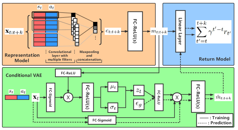
To derive a practical algorithm, an effective and compact representation function is necessary because: 1) the trajectory may have variant length, 2) and there may be irrelevant features in states and actions which might affect the estimation of the cumulative discounted reward of the trajectory. In this paper, we propose using Convolutional Neural Networks (CNNs) to learn a representation model $f^{\rm CNN}$ of state-action trajectory, similar to the use in sentence classification [13]. In our experiments, we found that this way achieves faster training and better performance than the popular LSTM [10] structure (see ablations in Section 6.2). An illustration of $f^{\rm CNN}$ is shown in the orange part of Figure 1.

Let $\textbf{x}_{t}\in\mathbb{R}^{l}$ be the $l$-dimensional feature vector of $(s_{t},a_{t})$ pair. A trajectory $\tau_{t:t+k}$ (padded where necessary) is represented as $\textbf{x}_{t:t+k}=\textbf{x}_{t}\oplus\textbf{x}_{t+1}\oplus\dots\oplus\textbf{x}_{t+k}$, where $\oplus$ is the concatenation operator. With a convolution filter $\textbf{w}^{i}\in\mathbb{R}^{h^{i}\times l}$ applied to a window of $h^{i}$ state-action pairs and then a max-pooling operation, a feature $c^{i}_{t:t+k}$ can be generated as follows:

$$c^{i}_{j}={\rm ReLU}(\textbf{w}^{i}\cdot \textbf{x}_{j:j+h^{i}-1}+b)\ {\rm where}\ j=t,\dots,t+k-h^{i}+1,$$ (7)

$$c^{i}_{t:t+k}=\max\{c^{i}_{t},c^{i}_{t+1}\dots,c^{i}_{t+k-h^{i}+1}\}.$$

We apply multiple filters ${\{\textbf{w}^{i}}\}_{i=1}^{n}$ on $\tau_{t:t+k}$ similarly to generate the $n$-dimensional feature vector $c_{t:t+k}$, then obtain the trajectory representation $m_{t:t+k}$ after several fully-connected layers:

$$c_{t:t+k}=(c^{1}_{t:t+k},c^{2}_{t:t+k},\dots,c^{n}_{t:t+k}),$$ (8)

$$m_{t:t+k}= f^{\rm CNN}(\tau_{t:t+k})={\rm FullyConnectedLayers}(c_{t:t+k}).$$

4.2 Trajectory Return Model

Following Lemma 1, we implement the trajectory return function $U$ with convex functions. Without loss of optimality, we use a linear $U$ to ensure the strict equality, as illustrated in the blue part of Figure 1. The result for a popular ReLU-activated layer can be seen in Ablation (Section 6.2).

We train the representation model $f^{\rm CNN}$ and return model $U^{\rm Linear}$ together by minimizing the mean square error loss of mini-batch samples from experience buffer $\mathcal{D}$, with respect to the parameters $\omega$:

$$\mathcal{L}^{\rm Ret}(\omega)=\mathbb{E}_{(\tau_{t:t+k},r_{t:t+k})\sim\mathcal{D}}\Big{[}\big{(}U^{\rm Linear}(f^{\rm CNN}(\tau_{t:t+k}))-\sum_{t^{\prime}=t}^{t+k}\gamma^{t^{\prime}-t}r_{t^{\prime}}\big{)}^{2}\Big{]}.$$ (9)

4.3 Conditional Variational Dynamics Model

The most straightforward way to implement the predictive dynamics function is to use a Multi-Layer Perceptron (MLP) $P^{\rm MLP}$ that takes the state and action as input and predicts the expected representation of future trajectory. However, such approach does not really model the stochasticity of future trajectory representation. In this paper, we present a conditional Variational Auto-Encoder (VAE) [14] to model the underlying distribution of future trajectory representation conditioned on the state and action, achieving significant improvement over $P^{\rm MLP}$ (see Ablation in Section 6.2).

The conditional VAE consists of two networks, an encoder $q_{\phi}(z_{t}|m_{t:t+k},s_{t},a_{t})$ and decoder $p_{\varphi}(m_{t:t+k}|z_{t},s_{t},a_{t})$ with variational parameters $\phi$ and generative parameters $\varphi$ respectively. With a chosen prior, generally the multivariate normal distribution $\mathcal{N}(0,I)$, the encoder approximates the conditional posteriors of latent variable $z_{t}$ for trajectory representation, producing a Gaussian distribution with mean $\mu_{t}$ and standard deviation $\sigma_{t}$. The decoder generates a representation of future trajectory $\tilde{m}_{t:t+k}$ for a given latent variable conditioned on the state-action pair. Besides, we use a pairwise-product operation to emphasize an explicit relation between the condition stream and trajectory representation stream, which shows better inference results in our experiments (see Ablation in Section 6.2). The structure of conditional VAE is illustrated in the green part of Figure 1.

During training, the latent variable is sampled from $\mathcal{N}(\mu_{t},\sigma_{t})$ with reparameterization trick [14], i.e., $z_{t}=\mu_{t}+\sigma_{t}\cdot\mathcal{N}(0,I)$, which is taken as part of input by the decoder to reconstruct the trajectory representation. This naturally models the underlying stochasticity of future trajectory. We train the conditional VAE with respect to the variational lower bound [14], in a form of the reconstruction loss along with a KL divergence term (see the Supplementary Material for complete formulation):

$$\mathcal{L}^{\rm VAE}(\phi,\varphi)=\mathbb{E}_{\tau_{t:t+k}\sim\mathcal{D}}\Big{[}\|m_{t:t+k}-\tilde{m}_{t:t+k}\|_{2}^{2}+\beta D_{\rm KL}\big{(}\mathcal{N}(\mu_{t},\sigma_{t})\|\mathcal{N}(0,I)\big{)}\Big{]},$$ (10)

where $m_{t:t+k}$ is obtained from the representation model (Equation 8). We use a weight $\beta>1$ to encourage VAE to discover disentangled latent factors for better inference quality, which is also known as a $\beta$-VAE [4, 9]. See Ablation (Section 6.2) for the results of different values of $\beta$.

Since VAE infers the latent distribution via instance-to-instance reconstruction, during the generation process, we propose using a clipped generative noise to narrow down the discrepancy between the generated instance and the expected representation (Equation 4). This allows us to obtain high-quality prediction of expected future trajectory. Finally, the predictive dynamics model $P^{\rm VAE}$ can be viewed as the generation process of the conditional VAE with a clipped generative noise $\epsilon_{g}$:

$$\tilde{m}_{t:t+k}=P^{\rm VAE}(s,a,\epsilon_{g}),{\rm and}\ \epsilon_{g}\sim{\rm Clip}\big{(}\mathcal{N}(0,I),-c,c\big{)}.$$ (11)

When $c$ is zero, an expected representation of future trajectory (Equation 4) should be generated from the mean of the latent distribution. A further discussion of clip value $c$ is in Ablation (Section 6.2).

4.4 Overall Algorithm

We build our algorithm on Deep Deterministic Policy Gradient (DDPG) [16] algorithm, by replacing the original critic (i.e., the $Q$-function) with a decomposed one, consisting of the three models introduced in previous subsections. The actor is updated through gradient ascent (Equation 6) similarly with respect to the decomposed critic. Note our algorithm does not use target networks for both the actor and critic. The overall algorithm is summarized in Algorithm 1.

Algorithm 1 Value decomposed DDPG with future prediction (VDFP) algorithm

1:Initialize actor network $\pi_{\theta}$ with random parameters $\theta$, and experience buffer $D$

2:Initialize representation model and trajectory return model with random parameters $\omega$

3:Initialize conditional VAE with random parameters $\phi$, $\varphi$

4:for episode $=1,2,\dots$ do

5:     for $t=1,2,\dots,T$ do

6:         Observe state $s_{t}$ and select action $a_{t}=\pi_{\theta}(s_{t})+\epsilon_{\rm e}$, with exploration noise $\epsilon_{\rm e}\sim\mathcal{N}(0,\sigma)$

7:         Execute action $a_{t}$ and obtain reward $r_{t}$

8:         Sample mini-batch of $N$ experience $\{(\tau_{t_{i}:T})\}_{i=1}^{N}$ from $\mathcal{D}$

9:         Update conditional VAE by minimizing $\mathcal{L}^{\rm VAE}(\phi,\varphi)$

10:         Predict the representation of future trajectory $\tilde{m}=P^{\rm VAE}(s,a,\epsilon_{g})|_{s=s_{i},a=\pi_{\theta}(s_{i})}$

11:         Update actor $\pi_{\theta}$ with the value-decomposed deterministic policy gradient (Equation 6)

12:     end for

13:     Store experiences $\{(\tau_{t:T},r_{t:T})\}_{t=1}^{T}$ in $\mathcal{D}$

14:     for epoch $=1,2,\dots$, num_epoch do

15:         Sample mini-batch of $N$ experience $\{(\tau_{t_{i}:T},r_{t_{i}:T})\}_{i=1}^{N}$ from $\mathcal{D}$

16:         Update representation model $f^{\rm CNN}$ and return model $U^{\rm Linear}$ by minimizing $\mathcal{L}^{\rm Ret}(\omega)$

17:     end for

18:end for

5 Related Work

Future Prediction

Thinking about the future has been considered as an integral component of human cognition [1, 20]. In neuroscience, one concept named the prospective brain [19] indicates that a crucial function of the brain is to use stored information to predict possible future events. The idea of future prediction is also studied in model-based RL [2, 26]. Simulated Policy Learning [11] is proposed to learn one-step predictive models from the real environment and then train a policy within the simulated environment. Multi-steps and long-term future are also modeled in [8, 12] with recurrent variational dynamics models, after which actions are chosen through online planning with Model-Predictive Control (MPC). Besides, another related work is [5], in which a supervised model is trained to predict the residuals of goal-related measurements at a set of temporal offsets in the future. With a manually designed goal vector, actions are chosen to maximize the predicted outcomes.

Value Function Approximation

Most model-free deep RL algorithms approximate value functions directly with deep neural networks, e.g., Proximal Policy Optimization (PPO) [23], Advantage Actor-Critic (A2C) [17] and DDPG [16], without explicitly handling the coupling of environmental dynamics and rewards. One similar approach to our work is the Deep Successor Representation (DSR) [15], which factors the value function into the dot-product between the expected representation of state occupancy and a vector of immediate reward function. The representation is trained with TD algorithm [27] and the vector is approximated from one-step transitions. In our work, we decompose the value function based on the composite form of trajectory dynamics and returns. In contrast to using TD algorithm, we use a conditional VAE to model the latent distribution and obtain expected trajectory representation. We demonstrate the superiority of our algorithm in the experimental section.

6 Experiments

We conduct our experiments on MuJoCo continuous control tasks in OpenAI gym [3, 28]. For the convenience of reproducibility, we make no modifications to the original environments or reward functions (except the delay reward modification in Section 6.3). Open source code and learning curves are provided in the Supplementary Material and will soon be released on GitHub.

6.1 Evaluation

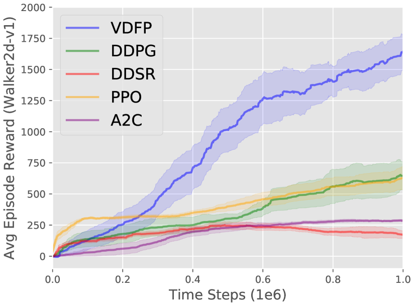
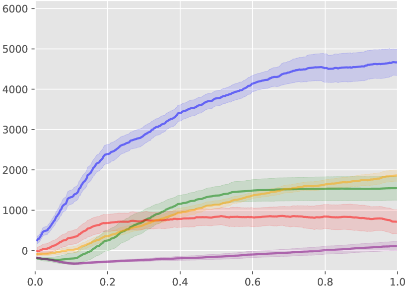
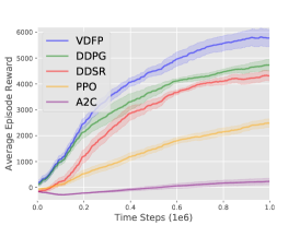
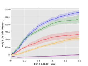
To evaluate the effectiveness of our algorithm, we focus on two representative MuJoCo tasks: HalfCheetah-v1 and Walker2d-v1, as adopted in [7, 6, 21, 23]. We compare our algorithm (VDFP) against DDPG, PPO, A2C, as well as the Deterministic DSR (DDSR). For PPO and A2C, we adopt non-parallelization implementation and use Generalized Advantage Estimation [22] with $\lambda=0.95$ for stable policy gradient. Since DSR is originally proposed based on DQN [18] for discrete action problems, we implement DDSR based on DDPG according to the author’s codes for DSR on GitHub. For VDFP, we set the KL weight $\beta$ as 1000 and the clip value $c$ as 0.2. We use the max trajectory length of 64 and 256 for HalfCheetah-v1 and Walker2d-v1 respectively. For VDFP, DDPG and DDSR, a Gaussian noise sampled from $\mathcal{N}(0,0.1)$ [7] is added to each action for exploration. For all algorithms, we use a two-layer feed-forward neural network of 200 and 100 hidden units with ReLU activation for both the actor and critic (similar scales for the critic variants in DDSR and VDFP).

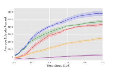
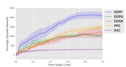
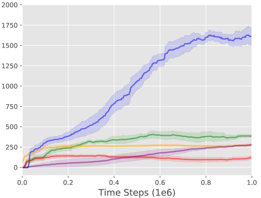
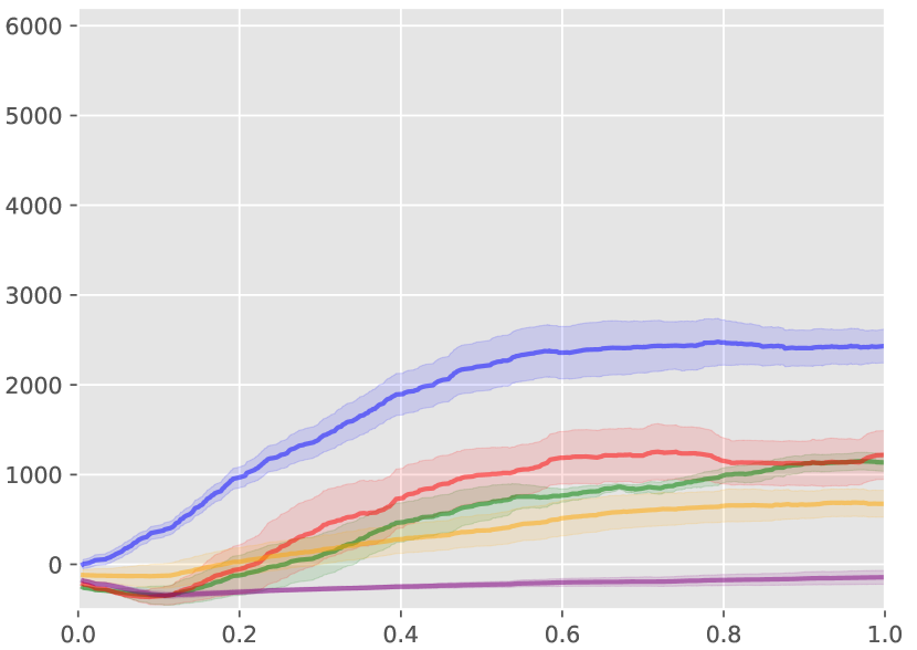
Figure 2 shows learning curves of algorithms over 5 random seeds of the Gym simulator and the network initialization. We can observe that our algorithm (VDFP) outperforms other algorithms in both final performance and learning speed. Our results for DDPG, PPO and A2C are comparable with those in [7, 23], where other results for ACKTR [29] and TRPO [21] can also been found. Exact experimental details of each algorithm are provided in the Supplementary Material.

(a) HalfCheetah-v1

(b) Walker2d-v1

Figure 2: Learning curves of algorithms in MuJoCo tasks. The shaded region denotes half a standard deviation of average evaluation over 5 trials. Results are smoothed over recent 100 episodes.

6.2 Ablation

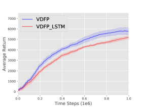
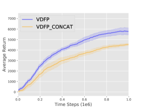
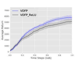
We perform ablation studies to analyze the contribution of each component of VDFP: 1) CNN (v.s. LSTM) for trajectory representation model (Representation); 2) conditional VAE (v.s. MLP) for predictive dynamics model (Architecture); 3) pairwise-product (v.s. concatenation) operation for conditional encoding process (Operator); and 4) a single linear layer (v.s. ReLU-activated layers) for trajectory return model (Return). We use the same experimental setups in Section 6.1 and the results are presented in Table 1. Complete learning curves can be found in the Supplementary Material.

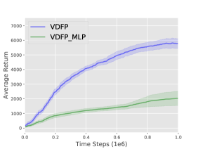
First, we can observe that CNN achieves better performance than LSTM. Actually, CNN also shows lower training losses and takes less practical training time (almost 8x faster) in our experiments. Second, the significance of conditional VAE is demonstrated by its superior performance over MLP. This is because it is difficult for MLP to approximate the expected representation from various trajectory instances. In contrast, conditional VAE can well capture the trajectory distribution and then obtain the expected representation through the generation process. Third, pairwise-product shows an obvious improvement over concatenation. We suggest that the explicit relation between the condition and representation imposed by pairwise-product, forces the conditional VAE to learn more effective hidden features. Lastly, adopting linear layer for the trajectory return model outperforms the case of using ReLU-activated layers since it ensures the equality between the composite function approximation and the $Q$-function (Lemma 1), thus obtains a better guarantee for the optimal policy.

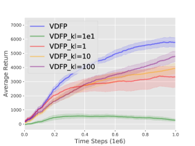
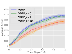
Moreover, we analyse the influence of weight $\beta$ for KL loss term (Equation 10) and clip value $c$ for prediction process (Equation 11). The results for different values of $\beta$ are consistent to the studies about $\beta$-VAE [4, 9]: larger $\beta$ applies stronger emphasis on VAE to discover disentangled latent factors, resulting in better inference performance. For clip value $c$, clipping achieves superior performance than not clipping ($c=\infty$) since this narrows down the discrepancy between prediction instance and expected representation of future trajectory as we discussed in Section 4.3. Though the complete clipping ($c=0.0$) should ensure the consistence to the expected representation and shows a good performance and lower deviation, considering the imperfect approximation of neural networks, setting $c$ to a small positive value ($c=0.2$) actually achieves a slightly better result.

Table 1: Ablation of VDFP across each contribution in HalfCheetah-v1. Results are Max Average Episode Reward over 5 trials of 1 million time steps. $\pm$ corresponds to half a standard deviation. Note that Operator, KL weight and clip value are not applicable (N/A) for the MLP architecture here.

Representation		Architecture		Operator		Return
CNN	LSTM	VAE	MLP	Pairwise-Prod.	Concat.	Linear	ReLU	$\beta$	$c$	Results
✓		✓		✓		✓		1000	0.2	5818.60 $\pm$  336.25
	✓	✓		✓		✓		1000	0.2	5197.03 $\pm$  156.52
✓			✓	N/A	N/A	✓		N/A	N/A	2029.00 $\pm$  486.11
✓		✓			✓	✓		1000	0.2	4541.71 $\pm$  104.22
✓		✓		✓			✓	1000	0.2	5119.04 $\pm$  390.89
✓		✓		✓		✓		100	0.2	4794.96 $\pm$  370.02
✓		✓		✓		✓		10	0.2	3933.33 $\pm$  361.82
✓		✓		✓		✓		1000	$\infty$	4752.84 $\pm$ 328.75
✓		✓		✓		✓		1000	0.0	5712.55 $\pm$  233.74

6.3 Delayed Reward

We further demonstrate the significant effectiveness and robustness of VDFP under delayed reward settings. We consider two representative delayed reward settings in real-world scenarios: 1) multi-step accumulated rewards are given at sparse time steps; 2) each one-step reward is delayed for certain time steps. To simulate above two settings, we make a simple modification to MuJoCo tasks respectively: 1) deliver $d$-step accumulated reward every $d$ time steps and at the end of an episode; 2) delay the immediate reward of each step by $d$ steps and compensate at the end of episode.

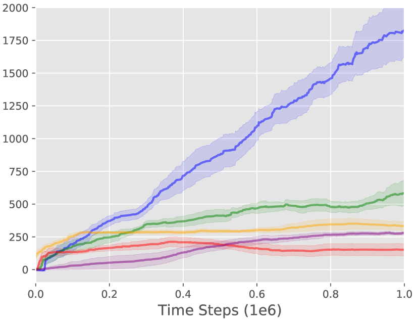
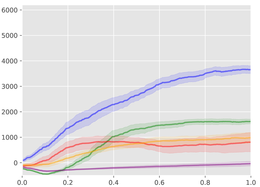
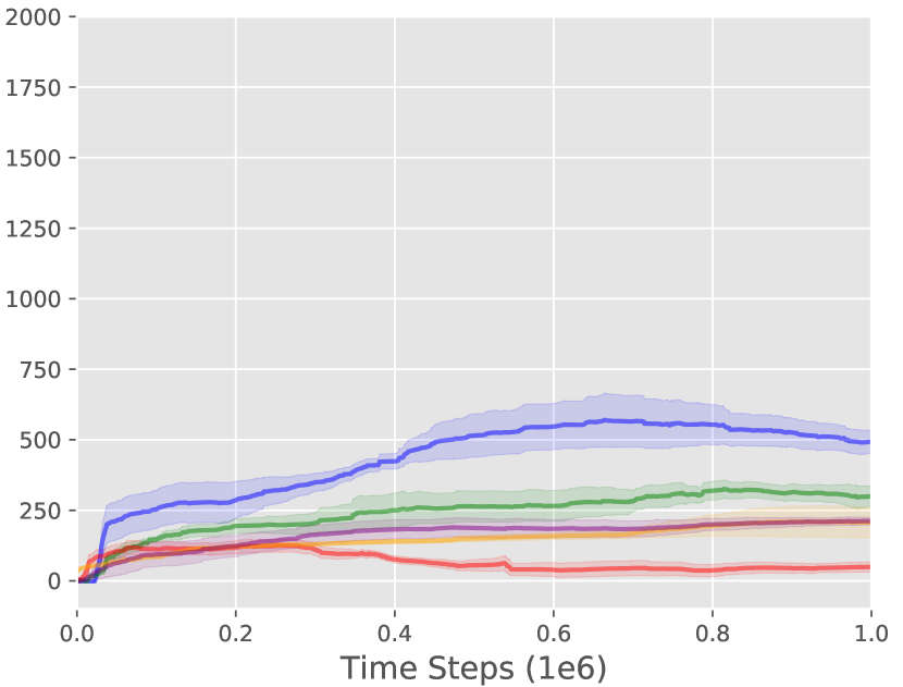
With the same experimental setups in Section 6.1, we evaluate the algorithms under different delayed reward settings, with a delay step $d$ from 16 to 128. For VDFP, a max trajectory length of 256 is used for all settings except that using 64 for HalfCheetah-v1 with $d=$ 16 and 32 already ensures a good performance. Figure 3 plots the results under the first delayed reward setting. Similar results are also observed for the second class of delay reward and can be found in the Supplementary Material.

As the increase of delay step $d$, all algorithms gradually degenerate in comparison with Figure 2 ($d=0$). DDSR can hardly learn effective policies under such delayed reward settings due to the failure of its one-step reward model even with a relatively small delay step (e.g., $d$ = 16). VDFP consistently outperforms others under all settings, in both learning speed and final performance (2x to 4x than DDPG). Besides, VDFP shows good robustness with delay step $d\leq 64$. As discussed in Section 3, we suggest that the reason for the superior performance of VDFP is two-fold: 1) VDFP can always learn the dynamics of the environment effectively from state and action feedbacks, which is irrelevant with how rewards are delayed actually; 2) the trajectory return model is robust with delayed reward since it approximates the cumulative reward instead of one-step immediate reward.

(a) delay step $d$ = 16

(b) delay step $d$ = 32

(c) delay step $d$ = 64

(d) delay step $d$ = 128

Figure 3: Learning curves under the first delayed reward setting. Different delay steps are listed from left to right. The upper and lower rows are for HalfCheetah-v1 and Walker2d-v1 respectively.

7 Conclusion and Future Work

We present an explicit two-step understanding of value functions in model-free RL from the perspective of future prediction. Through re-writing the value function in a composite function form, we decompose the value estimation process into two separate parts, which allows more effective and flexible use in different problems. Further, we derive our algorithm from such decomposition and innovatively propose a conditional variational dynamics model with clipped generation noise to predict the future. Evaluation and ablation studies are conducted in MuJoCo continuous control tasks. The effectiveness and robustness are also demonstrated under challenging delay reward settings.

In this paper, we use a off-policy training for VDFP and it could be flawed since trajectories collected by old policies may not able to represent the future under current policy. However, we do not observe any adverse effect of using off-policy training in our experiments (similar results are also found in [5]), and explicitly introducing several on-policy correction approaches shows no apparent benefits. We hypothesize that it is because the deterministic policy used in VDFP relaxes the on-policy requirements. It is worthwhile further investigation of this issue and the extension to stochastic policy. Besides, to some extend, the variational predictive dynamics model of VDFP can be viewed as a Monte Carlo (MC) based estimation [27] over the space of trajectory representation. In traditional RL approaches, MC value estimation are widely known to suffer from high variance. Thus, we suggest that VDFP may indicate a new variational MC approach with lower variance. We consider the theoretical analysis of the variance reduction as another future work.

A. Complete Learning Curves

A.1. Learning Curves for the Results in Ablation

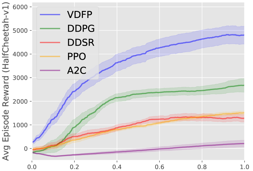
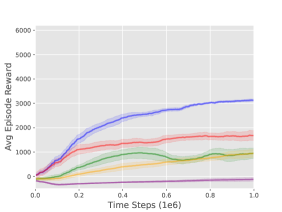
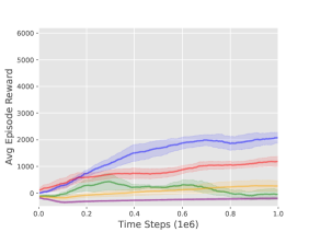
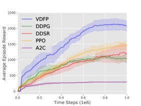
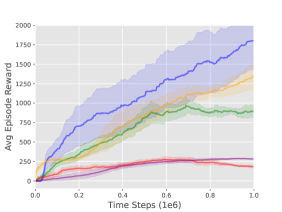
Figure 4 shows the learning curves of VDFP and its variants for ablation studies (Section 6.2), corresponding to the results in Table 1.

(a) VAE v.s. MLP

(b) CNN v.s. LSTM

(c) Pairwise-Prod. v.s. Concat.

(d) Linear v.s. ReLU

(e) KL weights

(f) Clip value

Figure 4: Learning curves of ablation studies for VDFP (i.e., VAE + CNN + Pairwise-Product + linear layer + kl=1000 + c=0.2) in HalfCheetah-v1. The shaded region denotes half a standard deviation of average evaluation over 5 trials. Results are smoothed over recent 100 episodes.

A.2. Results for the Second Delayed Reward Setting

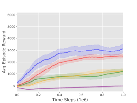
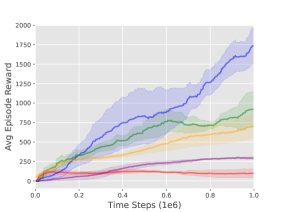
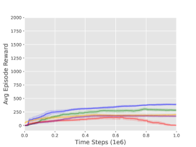
We use the second delayed reward setting to model the representative delay reward in real-world scenarios: each one-step reward is delayed for certain time steps. We make a simple modification to MuJoCo tasks to simulate such class of delay reward: delay the immediate reward of each step by $d$ steps and compensate at the end of episode. The complete learning curves of algorithms under the second delay reward setting are shown in Figure 5 and 6. All algorithms gradually degenerate with the increase of delay step $d$. VDFP consistently outperforms others under all settings, and shows good robustness with delay step $d\leq 64$.

(a) delay step $d$ = 0

(b) delay step $d$ = 16

(c) delay step $d$ = 32

(d) delay step $d$ = 64

(e) delay step $d$ = 128

Figure 5: Learning curves of algorithms in HalfCheetah-v1 under the second delayed reward setting. Different delay steps are listed from left to right. The shaded region denotes half a standard deviation of average evaluation over 5 trials. Results are smoothed over recent 100 episodes.

(a) delay step $d$ = 0

(b) delay step $d$ = 16

(c) delay step $d$ = 32

(d) delay step $d$ = 64

(e) delay step $d$ = 128

Figure 6: Learning curves of algorithms in Walker2d-v1 under the second delayed reward setting. Different delay steps are listed from left to right. The shaded region denotes half a standard deviation of average evaluation over 5 trials. Results are smoothed over recent 100 episodes.

B. Experimental Details

B.1. Environment Setup

We conduct our experiments on MuJoCo continuous control tasks in OpenAI gym. We use the OpenAI gym with version 0.9.1, the mujoco-py with version 0.5.4 and the MuJoCo products with version MJPRO131. Our codes are implemented with Python 3.6 and Tensorflow 1.8. Our code and raw learning curves are submitted under review, and will be released on GitHub soon.

B.2. Network Structure

As shown in Table 2, we use a two-layer feed-forward neural network of 200 and 100 hidden units with ReLU activation (except for the output layer) for the actor network for all algorithms, and for the critic network for DDPG, PPO and A2C. For PPO and A2C, the critic denotes the $V$-network.

Table 2: Network structures for the actor network and the critic network ($Q$-network or $V$-network).

Layer	Actor Network ($\pi(s)$)	Critic Network ($Q(s,a)$ or $V(s)$)
Fully Connected	(state dim, 200)	(state dim, 200)
Activation	ReLU	ReLU
Fully Connected	(200, 100)	(action dim + 200, 100) or (200, 100)
Activation	ReLU	ReLU
Fully Connected	(100, action dim)	(100, 1)
Activation	tanh	None

For DDSR, the factored critic (i.e., $Q$-function) consists of a representation network, a reconstruction network, a SR network and a linear reward vector, as described in the original paper of DSR. The structure of the factored critic of DDSR is shown in Table 3.

Table 3: The Network structure for the factored critic network of DDSR, including a representation network, a reconstruction network, a SR network and a reward vector.

Network	Layer	Structure
Representation Network	Fully Connected	(state dim, 200)
	Activation	ReLU
	Fully Connected	(200, 100)
	Activation	ReLU
	Fully Connected	(100, representation dim)
	Activation	None
Reconstruction Network	Fully Connected	(representation dim, 100)
	Activation	ReLU
	Fully Connected	(100, 200)
	Activation	ReLU
	Fully Connected	(200, state dim)
	Activation	None
SR Network	Fully Connected	(representation dim, 200)
	Activation	ReLU
	Fully Connected	(200, 100)
	Activation	ReLU
	Fully Connected	(100, representation dim)
	Activation	None
Linear Reward Vector	Fully Connected (not use bias)	(representation dim, 1)
	Activation	None

For VDFP, the decomposed critic (i.e., $Q$-function) consists of a convolutional representation network $f^{\rm CNN}$, a linear trajectory return network $U^{\rm Linear}$ and a conditional VAE (an encoder network and a decoder network). The structure of the decomposed critic of VDFP is shown in Table 4.

Table 4: The Network structure for the factored critic network of VDFP, including a convolutional representation network $f^{\rm CNN}$, a linear trajectory return network $U^{\rm Linear}$ and a conditional VAE (an encoder network and a decoder network).

Network	Layer (Name)	Sturcture
Representation Network	Convolutional	filters with height $\in\{1,2,4,8,16,32,64\}$
$f^{\rm CNN}(\tau_{t:t+k})$		of numbers $\{20,20,10,10,5,5,5\}$
	Activation	ReLU
	Pooling (concat)	Maxpooling & Concatenation
	Fully Connected (highway)	(filter num, filter num)
	Joint	Sigmoid(highway) $\cdot$ ReLU(highway)
		+ (1 - Sigmoid(highway)) $\cdot$ ReLU(concat)
	Dropout	Dropout(drop_prob = 0.2)
	Fully Connected	(filter num, representation dim)
	Activation	None
Conditional Encoder Network	Fully Connected (main)	(representation dim, 400)
$q_{\phi}(z_{t}|m_{t:t+k},s_{t},a_{t})$	Fully Connected (encoding)	(state dim + action dim, 400)
	Pairwise-Product	Sigmoid(encoding) $\cdot$ ReLU(main)
	Fully Connected	(400, 200)
	Activation	ReLU
	Fully Connected (mean)	(200, $z$ dim)
	Activation	None
	Fully Connected (log_std)	(200, $z$ dim)
	Activation	None
Conditional Decoder Network	Fully Connected (latent)	(z dim, 200)
$p_{\varphi}(m_{t:t+k}|z_{t},s_{t},a_{t})$	Fully Connected (decoding)	(state dim + action dim, 200)
	Pairwise-Product	Sigmoid(decoding) $\cdot$ ReLU(latent)
	Fully Connected	(200, 400)
	Activation	ReLU
	Fully Connected (reconstruction)	(400, representation dim)
	Activation	None
Trajectory Return Network	Fully Connected	(representation dim, 1)
$U^{\rm Linear}(m_{t:t+k})$	Activation	None

For VDFP_MLP, we also use a two-layer feed-forward neural network of 200 and 100 hidden units with ReLU activation (except for the output layer) for $P^{\rm MLP}$. For VDFP_LSTM, we use one LSTM layer with 100 units to replace the convolutional layer (along with maxpooling layer) as described in Table 4. For VDFP_Concat, we concatenate the state, action and the representation (or latent variable) rather than a pairwise-product structure. For VDFP_ReLU, we add an ReLU-activated fully-connected layer with 50 units in front of the linear layer for trajectory return model.

B.3. Hyperparameter

For all our experiments, we use the raw observation and reward from the environment and no normalization or scaling are used. No regularization is used for the actor and the critic in all algorithms. Table 5 shows the common hyperparamters of algorithms used in all our experiments. For VDFP and DDSR, critic learning rate denotes the learning rate of the conditional VAE and the successor representation model respectively. Return (reward) model learning rate denotes the learning rate of the return model (along with the representation model) for VDFP and the learning rate of the immediate reward vector for DDSR.

Table 5: A comparison of common hyperparameter choices of algorithms. We use ‘-’ to denote the ‘not applicable’ situation.

Hyperparameter	VDFP	DDSR	DDPG	PPO	A2C
Actor Learning Rate	2.5$\cdot$10-4	2.5$\cdot$10-4	10-4	10-4	10-4
Critic (VAE, SR) Learning Rate	10-3	10-3	10-3	10-3	10-3
Return (Reward) Model Learning Rate	5$\cdot$10-4	5$\cdot$10-4	-	-	-
Discount Factor	0.99	0.99	0.99	0.99	0.99
Optimizer	Adam	Adam	Adam	Adam	Adam
Target Update Rate	-	10-3	10-3	-	-
Exploration Policy	$\mathcal{N}(0,0.1)$	$\mathcal{N}(0,0.1)$	$\mathcal{N}(0,0.1)$	None	None
Batch Size	64	64	64	256	256
Buffer Size	105	105	105	-	-
Actor Epoch	-	-	-	10	10
Critic Epoch	-	-	-	10	10

B.4. Additional Implementation Details

For DDPG, the actor network and the critic network is updated every 1 time step. We implement the DDSR based on the DDPG algorithm, by replacing the original critic of DDPG with the factored $Q$-function as described in the DSR paper. The actor, along with all the networks described in Table 3 are updated every 1 time step. The representation dimension is set to 100. Before the training of DDPG and DDSR, we run 10000 time steps for experience collection, which are also counted in the total time steps.

For PPO and A2C, we use Generalized Advantage Estimation with $\lambda=0.95$ for stable policy gradient. The clip range of PPO algorithm is set to 0.2. The actor network and the critic network are updated every $2$ and $5$ episodes for HalfCheetah-v1 and Walker2d-v1 respectively, with the epoches and batch sizes described in Table 5.

For VDFP, we set the KL weight $\beta$ as 1000 and the clip value $c$ as 0.2. The latent variable dimension ($z$ dim) is set to 50 and the representation dimension is set to 100. We collect trajectories experiences in the first 5000 time steps and then pre-train the trajectory model (along with the representation model) and the conditional VAE for 15000 time steps, after which we start the training of the actor. All the time steps above are counted into the total time steps for a fair comparison. The trajectory return model (along with the representation model) is trained every 10 time steps for the pre-train process and is trained every 50 time steps in the rest of training, which already ensures a good performance in our experiments. The actor network and the conditional VAE are trained every 1 time step.

We consider a max trajectory length $l$ for VDFP in our experiments. For example, a max length $l$ = 256 can be considered to correspond a discounted factor $\gamma=0.99$ as $0.99^{256}\approx 0.076$. In practice, for a max length $l>64$, we add an additional fully-connected layer with ReLU activation before the convolutional representation model $f^{\rm CNN}$, to aggregate the trajectory into the length of 64. This is used for the purpose of reducing the time cost and accelerating the training of the convolutional representation model as described in Table 4. For example, we feed every 4 state-action pairs of a trajectory with length 256 into the aggregation layer to obtain an aggregated trajectory with the length 64, and then feed the aggregated trajectory to $f^{\rm CNN}$ for a trajectory representation.

C. Complete Formulation for the conditional VAE

A variational auto-encoder (VAE) is a generative model which aims to maximize the marginal log-likelihood $\log p(X)=\sum_{i=1}^{N}\log p(x_{i})$ where $X=\{x_{1},\dots,x_{N}\}$, the dataset. While computing the marginal likelihood is intractable in nature, it is a common choice to train the VAE through optimizing the variational lower bound:

$$\log p(X)\geq\mathbb{E}_{q(X|z)}[\log p(X|z)]+D_{\rm KL}\big{(}q(z|X)\|p(z)\big{)},$$ (12)

where $p(z)$ is chosen a prior, generally the multivariate normal distribution $\mathcal{N}(0,I)$.

In our paper, we use a conditional VAE to model the latent distribution of the representation of future trajectory conditioned on the state and action, under certain policy. Thus, the true parameters of the distribution, denoted as $\varphi^{*}$, maximize the conditional log-likelihood as follows:

$$\varphi^{*}=\arg\max_{\varphi}\sum_{i=1}^{N}\log p^{\pi}_{\varphi}(m_{t:t+k}|s_{t},a_{t}).$$ (13)

The likelihood can be calculated with the prior distribution of latent variable $z$:

$$p^{\pi}_{\varphi}(m_{t:t+k}|s_{t},a_{t})=\int p^{\pi}_{\varphi}(m_{t:t+k}|z_{t},s_{t},a_{t})p^{\pi}_{\varphi}(z_{t}){\rm d}z.$$ (14)

Since the prior distribution of latent variable $z$ is not easy to compute, an approximation of posterior distribution $q^{\pi}_{\phi}(z_{t}|m_{t:t+k},s_{t},a_{t})$ with parameterized $\phi$ is introduced.

The variational lower bound of such a conditional VAE can be obtained as follows, superscripts and subscripts are omitted for clarity:

$$D_{\rm KL} \big{(}q_{\phi}(z|m,s,a)\|p_{\varphi}(z|m,s,a)\big{)}$$ (15)

$$=\int q_{\phi}(z|m,s,a)\log\frac{q_{\phi}(z|m,s,a)}{p_{\varphi}(z|m,s,a)}{\rm d}z$$

$$=\int q_{\phi}(z|m,s,a)\log\frac{q_{\phi}(z|m,s,a)p_{\varphi}(m|s,a)}{p_{\varphi}(z,m|s,a)}{\rm d}z$$

$$=\int q_{\phi}(z|m,s,a)\big{[}\log p_{\varphi}(m|s,a)+\log\frac{q_{\phi}(z|m,s,a)}{p_{\varphi}(z,m|s,a)}\big{]}{\rm d}z$$

$$=\log p_{\varphi}(m|s,a)+\int q_{\phi}(z|m,s,a)\log\frac{q_{\phi}(z|m,s,a)}{p_{\varphi}(z,m|s,a)}{\rm d}z$$

$$=\log p_{\varphi}(m|s,a)+\int q_{\phi}(z|m,s,a)\log\frac{q_{\phi}(z|m,s,a)}{p_{\varphi}(m|z,s,a)p_{\varphi}(z|s,a)}{\rm d}z$$

$$=\log p_{\varphi}(m|s,a)+\int q_{\phi}(z|m,s,a)\big{[}\log\frac{q_{\phi}(z|m,s,a)}{p_{\varphi}(z|s,a)}-\log p_{\varphi}(m|z,s,a)\big{]}{\rm d}z$$

$$=\log p_{\varphi}(m|s,a)+D_{\rm KL}\big{(}q_{\phi}(z|m,s,a)\|p_{\varphi}(z|s,a)\big{)}-\mathbb{E}_{z\sim q_{\phi}(z|m,s,a)}\log p_{\varphi}(m|z,s,a).$$

Re-arrange the above equation,

$$\log p_{\varphi}(m|s,a)- D_{\rm KL}\big{(}q_{\phi}(z|m,s,a)\|p_{\varphi}(z|m,s,a)\big{)}$$ (16)

$$=\mathbb{E}_{z\sim q_{\phi}(z|m,s,a)}\log p_{\varphi}(m|z,s,a)-D_{\rm KL}\big{(}q_{\phi}(z|m,s,a)\|p_{\varphi}(z|s,a)\big{)}.$$

Since the KL divergence is none-negative, we obtain the variational lower bound for the conditional VAE:

$$\log p_{\varphi}(m|s,a)\geq\log p_{\varphi}(m|s,a)-D_{\rm KL}\big{(}q_{\phi}(z|m,s,a)\|p_{\varphi}(z|m,s,a)\big{)}=-\mathcal{L}^{\rm VAE},$$ (17)

Thus, we can obtain the optimal parameters through optimizing the equation below:

$$\mathcal{L}^{\rm VAE}=-\mathbb{E}_{z\sim q_{\phi}(z|m,s,a)}\log p_{\varphi}(m|z,s,a) +D_{\rm KL}\big{(}q_{\phi}(z|m,s,a)\|p_{\varphi}(z|s,a)\big{)},$$ (18)

$$\phi^{*},\varphi^{*}= \arg\min_{\phi,\varphi}\mathcal{L}^{\rm VAE}.$$

$q_{\phi}(z|m,s,a)$ is the conditional variational encoder and the $\log p_{\varphi}(m|z,s,a)$ is the conditional variational decoder.

In our paper, we implement the encoder and decoder with deep neural networks. The encoder takes the trajectory representation and state-action pair as input and output a Gaussian distribution with mean $\mu_{t}$ and standard deviant $\sigma_{t}$, from which a latent variable is sampled and then feed into the decoder for the reconstruction of the trajectory representation. Thus, we train the conditional VAE with respect to the variational lower bound (Equation 18), in the following form:

$$\mathcal{L}^{\rm VAE}(\phi,\varphi)=\mathbb{E}_{\tau_{t:t+k}\sim\mathcal{D}}\Big{[}\|m_{t:t+k}-\tilde{m}_{t:t+k}\|_{2}^{2}+D_{\rm KL}\big{(}\mathcal{N}(\mu_{t},\sigma_{t})\|\mathcal{N}(0,I)\big{)}\Big{]}.$$ (19)

References

- [1] C. M. Atance and D. K. O’Neill. Episodic future thinking. Trends in Cognitive Sciences, 5:533–539, 2001.
- [2] C. G. Atkeson and S. Schaal. Robot learning from demonstration. In ICML, pages 12–20, 1997.
- [3] G. Brockman, V. Cheung, L. Pettersson, J. Schneider, J. Schulman, J. Tang, and W. Zaremba. Openai gym. CoRR, abs/1606.01540, 2016.
- [4] C. P. Burgess, I. Higgins, A. Pal, L. Matthey, N. Watters, G. Desjardins, and A. Lerchner. Understanding disentangling in -vae. CoRR, abs/1804.03599, 2018.
- [5] A. Dosovitskiy and V. Koltun. Learning to act by predicting the future. In ICLR, 2017.
- [6] S. Fujimoto, D. Meger, and D. Precup. Off-policy deep reinforcement learning without exploration. CoRR, abs/1812.02900, 2018.
- [7] S. Fujimoto, H. v. Hoof, and D. Meger. Addressing function approximation error in actor-critic methods. In ICML, 2018.
- [8] D. Hafner, T. P. Lillicrap, I. Fischer, R. Villegas, D. Ha, H. Lee, and J. Davidson. Learning latent dynamics for planning from pixels. CoRR, abs/1811.04551, 2018.
- [9] I. Higgins, L. Matthey, A. Pal, C. Burgess, X. Glorot, M. Botvinick, S. Mohamed, and A. Lerchner. beta-vae: Learning basic visual concepts with a constrained variational framework. In ICLR, 2017.
- [10] S. Hochreiter and J. Schmidhuber. Long short-term memory. Neural Computation, 9(8):1735–1780, 1997.
- [11] L. Kaiser, M. Babaeizadeh, P. Milos, B. Osinski, R. H. Campbell, K. Czechowski, D. Erhan, C. Finn, P. Kozakowski, S. Levine, R. Sepassi, G. Tucker, and H. Michalewski. Model-based reinforcement learning for atari. CoRR, abs/1903.00374, 2019.
- [12] N. R. Ke, A. Singh, A. Touati, A. Goyal, Y. Bengio, D. Parikh, and D. Batra. Learning dynamics model in reinforcement learning by incorporating the long term future. In ICLR, 2019.
- [13] Y. Kim. Convolutional neural networks for sentence classification. In EMNLP, pages 1746–1751, 2014.
- [14] D. P. Kingma and M. Welling. Auto-encoding variational bayes. In ICLR, 2014.
- [15] T. D. Kulkarni, A. Saeedi, S. Gautam, and S. J. Gershman. Deep successor reinforcement learning. CoRR, abs/1606.02396, 2016.
- [16] T. P. Lillicrap, J. J. Hunt, A. Pritzel, N. Heess, T. Erez, Y. Tassa, D. Silver, and D. Wierstra. Continuous control with deep reinforcement learning. In ICLR, 2015.
- [17] V. Mnih, A. P. Badia, M. Mirza, A. Graves, T. P. Lillicrap, T. Harley, D. Silver, and K. Kavukcuoglu. Asynchronous methods for deep reinforcement learning. In ICML, 2016.
- [18] V. Mnih, K. Kavukcuoglu, D. Silver, A. A. Rusu, J. Veness, M. G. Bellemare, A. Graves, M. A. Riedmiller, A. Fidjeland, G. Ostrovski, S. Petersen, C. Beattie, A. Sadik, I. Antonoglou, H. King, D. Kumaran, D. Wierstra, S. Legg, and D. Hassabis. Human-level control through deep reinforcement learning. Nature, 518(7540):529–533, 2015.
- [19] D. L. Schacter, D. R. Addis, and R. L. Buckner. Remembering the past to imagine the future: the prospective brain. Nature Reviews Neuroscience, 8:657–661, 2007.
- [20] D. L. Schacter and D. Rose Addis. The cognitive neuroscience of constructive memory: remembering the past and imagining the future. Philosophical transactions of the Royal Society of London. Series B, Biological sciences, 362 1481:773–86, 2007.
- [21] J. Schulman, S. Levine, P. Abbeel, M. I. Jordan, and P. Moritz. Trust region policy optimization. In ICML, pages 1889–1897, 2015.
- [22] J. Schulman, P. Moritz, S. Levine, M. I. Jordan, and P. Abbeel. High-dimensional continuous control using generalized advantage estimation. In ICLR, 2016.
- [23] J. Schulman, F. Wolski, P. Dhariwal, A. Radford, and O. Klimov. Proximal policy optimization algorithms. CoRR, abs/1707.06347, 2017.
- [24] D. Silver, A. Huang, C. J. Maddison, A. Guez, L. Sifre, G. Driessche, J. Schrittwieser, I. Antonoglou, V. Panneershelvam, M. Lanctot, S. Dieleman, D. Grewe, J. Nham, N. Kalchbrenner, I. Sutskever, T. P. Lillicrap, M. Leach, K. Kavukcuoglu, T. Graepel, and D. Hassabis. Mastering the game of go with deep neural networks and tree search. Nature, 529(7587):484–489, 2016.
- [25] D. Silver, G. Lever, N. Heess, T. Degris, D. Wierstra, and M. A. Riedmiller. Deterministic policy gradient algorithms. In ICML, pages 387–395, 2014.
- [26] R. S. Sutton. Dyna, an integrated architecture for learning, planning, and reacting. SIGART Bulletin, 2(4):160–163, 1991.
- [27] R. S. Sutton and A. G. Barto. Reinforcement learning: An introduction. IEEE Transactions on Neural Networks, 16:285–286, 1988.
- [28] E. Todorov, T. Erez, and Y. Tassa. Mujoco: A physics engine for model-based control. 2012 IEEE/RSJ International Conference on Intelligent Robots and Systems, pages 5026–5033, 2012.
- [29] Y. Wu, E. Mansimov, S. Liao, R. B. Grosse, and J. Ba. Scalable trust-region method for deep reinforcement learning using kronecker-factored approximation. In NIPS, 2017.