Inverse design of charged colloidal particle interactions for self assembly into specified crystal structures
Abstract
We study the inverse problem of tuning interaction parameters between charged colloidal particles interacting with a hard-core repulsive Yukawa potential, so that they assemble into specified crystal structures. Here, we target the body-centered-cubic (bcc) structure which is only stable in a small region in the phase diagram of charged colloids and is, therefore, challenging to find. In order to achieve this goal, we use the statistical fluctuations in the bond orientational order parameters to tune the interaction parameters for the bcc structure, while initializing the system in the fluid phase, using the Statistical Physics-inspired Inverse Design (SP-ID) algorithm Miskin . We also find that this optimization algorithm correctly senses the fluid-solid phase boundaries for charged colloids. Finally, we repeat the procedure employing the Covariance Matrix Adaptation - Evolution Strategy (CMA-ES), a cutting edge optimization technique, and compare the relative efficacy of the two methods.
I Introduction
In the past few years, several inverse methods have emerged that design optimal interactions in such a way that the system spontaneously assembles into a targeted structure Rechtsman0 ; Rechtsman1 ; Rechtsman2 ; Rechtsman3 . These methods have received considerable attention in materials science Torquato ; Jain ; Jaeger , and have been successively used to find crystal structures for photonic band-gap applications Ho , to predict crystals Oganov and protein structures Dahiyat ; Kuhlman , materials with optimal mechanical and transport properties Hyun , and for optimizing the interactions for self assembly Hannon0 ; Chang ; Rechtsman4 ; Hannon1 ; Hormoz . Though many of the methods developed are either based on black-box techniques, in which the algorithm tunes the interaction parameters without taking the statistical nature of the system into account, or are designed ad hoc for a particular class of systems, systematic approaches based on a statistical mechanical formulation, which are general, and allow for application tailored to specific systems of interest, have also been investigated.
In the present work, we investigate the efficacy of one such method, the Statistical Physics-inspired Inverse Design (SP-ID) method developed by Miskin et al Miskin . This method considers statistical fluctuations present in the microscopic configurations of the system for tuning the interactions between the particles. In order to design these interactions, we have used a quality function based on bond order parameters Stein ; Lechner to rank the generated configurations. The same task can be faced employing numerous optimization techniques like (Adaptive) Simulated Annealing Kirkpatrick ; Ingber1 ; Ingber2 , Particle Swarm Optimization DeOca , and several genetic algorithms Mitchell . To evaluate the effectiveness of the SP-ID algorithm, we compare it with the Covariance Matrix Adaption - Evolutionary Strategy (CMA-ES) Hansen2001 ; Hansen2003 ; Hansen2006 , which we regard as a state-of-the-art optimization technique for evolutionary computation.
We have chosen a system of colloidal particles as the model for which we wish to design the interactions in order to target a specific crystal structure. The interparticle potential of colloids offers a wide variety of functional forms. It can contain a hard-core term, a dipole-dipole term, a charge dispersion term, a screened-Coulomb (Yukawa) term and a short-ranged attractive depletion term. More specific designed colloidal particles such as patchy colloids and DNA-functionalized colloids offer even greater diversity of interactions. For all of these, the interaction parameters can be tuned. In the case of Yukawa interactions, the Debye screening length can be adjusted by changing the salt concentration, and the contact value can be tuned by altering the surface charge of the particles. Previous studies have employed what may be termed a forward method in which, starting from the microscopic interaction parameters and specified thermodynamic parameters such as temperature and density, one computes the equilibrium properties and finds the stable phase of the system. In the present work, our purpose is to employ an inverse method, where the target structure and equilibrium properties are the input from which we wish to design the interparticle interactions for which the particles spontaneously self assemble into the target structure.
In this study, we considered a charged colloidal system in which particles interact with a hard-core repulsive Yukawa potential. The complete phase diagram of hard-core Yukawa particles is known from earlier studies Meijer1 ; Meijer ; Dijkstra . Because of the purely repulsive nature of the potential, this system displays only a fluid phase which can freeze into a face-centered-cubic (fcc) or a body-centered-cubic (bcc) crystal phases. The phase diagram of hard-core Yukawa particles shows two triple points where fcc, bcc, and fluid phases coexist. The bcc phase is only stable in a very small region in the phase diagram and, for this reason, constitutes a reasonable test case for the reverse-engineering process. In this work, we search for optimal interparticle interactions which favor the crystallization of the bcc structure. Here we show three different cases, in which we respectively tune one, two and three parameters. In all cases, we show that both SP-ID and CMA-ES adjust the interparticle interactions that lead to the targeted bcc structure formation.
The paper is organized as follows: In Sec. II, we define the model system studied in this paper and the corresponding phase diagram and bond order parameters to identify the different phases. In Sec. III, we define the inverse design methods and the form of the quality function used in this study. Results for tuning the interactions to target the bcc structure for all three cases are discussed in Sec. IV. Finally, we summarize our results in Sec. V.
II Model and Simulation Methods
Interaction Potential: We consider a hard-core repulsive Yukawa system which represents a standard model for charged colloids. The form of the potential is given by
| (1) |
where is the contact value of the pair potential expressed in units of
, is the inverse of the Debye screening length, and is the
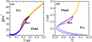
hard-core diameter. In Fig. 1, we show the phase diagram for such a system with in the representation and the plane Dijkstra . The phase diagram exhibits a stable fluid, bcc, and fcc region, as well as two triple points at which the three phases coexist. Note that we always use scaled variables, a reduced temperature , pressure and inverse screening length , each of which can be treated as tuning parameter for obtaining the desired behavior.
Bond order parameters (BOP): Every optimization algorithm, including SP-ID and CMA-ES, works on the basis of minimizing a user-defined fitness function. Here, we have used the averaged bond order parameters and (). The first is computed as follows: Stein ; Lechner ,
| (2) |
where,
Here, is the number of neighbors of particle , is the number of neighbors including particle itself, denotes the spherical harmonics with the distance vector from particle to particle . The second bond order parameter we used is defined as
In order to calculate the radius of the first coordination shell for each particle, we employ the solid angle based nearest-neighbor (SANN) algorithm Sann , where a nearest neighbor of a particle is identified by attributing a solid angle to each possible neighbor such that the sum of solid angles equals at least .
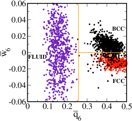
In Fig. 2, we show the scatter plots of versus for the fluid, bcc, and fcc phases of a system of Yukawa particles with at the high-density triple point conditions. We find distinct clouds of points corresponding to the fluid, bcc, and fcc phases, and hence, and can be used to distinguish the three phases.
III Inverse design Methods
III.1 Statistical Physics-inspired Inverse Design method
In the SP-ID method, microscopic parameters such as the interparticle pair potential parameters are tuned by exploiting statistical fluctuations in such a way that the system will evolve to those states which correspond to the targeted macroscopic response of that system, unlike other models which are entirely based on black-box techniques Miskin . In this method, the time evolution of the probability distribution of finding the system in configuration is written as
| (3) |
where denotes the probability of finding a system in some configuration, are the adjustable parameters and is a quality function which gives a weight/fitness value to each configuration based on a targeted macroscopic property. With straightforward manipulation, the above equation can be recast as equations of motion for Miskin :
| (4) | |||||
where denotes an ensemble average at a given set of values of .
To integrate Eq. 4, we have used a modified Euler method with a fixed time step of 4.0.
We have built our quality function in the following way:
| (5) |
where denotes the fitness function,
| (6) |
with and the averages of the bond order parameters over all the particles in the system, and and are the corresponding quantities in the target structure (bcc). Here, the integral over represents a sum over a series of different configurations as obtained from a simulation for a fixed set of parameters . The quality function will have higher values for those configurations whose and values are closer to the target values. More precisely, equals the probability of having a lower value of than any other configuration drawn randomly from the equilibrium distribution. To target the bcc structure, we have chosen and (average values of , for the bcc structure obtained from the scatter plot shown in Fig. 2). For a perfect bcc structure, these values are, and , but here we have targeted the bond order parameter values for a finite-temperature bcc structure.
III.2 Covariance Matrix Adaptation-Evolutionary Strategy
In order to implement CMA-ES, we draw samples from a multivariate Gaussian distribution for each generation whose dimension corresponds to the number of parameters we wish to tune. Subsequently, we evaluate the fitness function on the generated samples, and we pick the best samples. Using the following equations, we estimate the multivariate Gaussian distribution with mean (a -dimensional vector) and the covariance matrix of the Gaussian distribution for the next generation using:
| (7) | ||||
where denotes the samples consisting of multiple configurations calculated for different parameter sets (denoted by above) in CMA-ES, is the normalized distribution of weights based on the fitness of the samples. We choose where is the rank index of sample ( for the configuration with the smallest value) for the best samples, and set for the rest. and are additional -dimensional vectors which determine, respectively, the changes in amplitude and directionality of the covariance matrix, and finally is the average length of a vector drawn from a multivariate Gaussian distribution centered in the origin and where the covariance matrix is the identity matrix. In the present work we use and . For the first generation we initialize and as null vectors. Moreover, since we do not assume any a priori correlation between the different tuning parameters, the initial form of the covariance matrix is diagonal. Finally, all the free parameters of the CMA-ES are selected following the recipe in Ref. Hansen2006, .
Note that there is a substantial difference in the use of the fitness function between the two methods. In SP-ID we rank different configurations, so and are bond order parameters computed in a single configuration. The SP-ID method is thus based on the statistical fluctuations in the bond order parameters (Fig. 2) in a simulation at a single set of interaction parameters in order to optimize these values for the desired bcc structure. When using the CMA-ES, we rank samples, so and are computed as ensemble averages of these bond order parameters over multiple configurations for distinct sets of parameters. The CMA-ES method is thus based on a ranking of the different samples as obtained for different interaction parameter sets in order to optimize the parameter values.
III.3 Simulation details
In order to evaluate the ensemble averages and to generate distinct configurations for the SP-ID method, we perform constant pressure and constant temperature () Monte Carlo (MC) simulations on systems consisting of hard-core repulsive Yukawa particles. We initialize the simulations by placing the particles randomly in a cubic simulation box. We equilibrate the system up to MC cycles. One Monte Carlo cycle corresponds to particle moves and one volume move. The particle and volume moves are adjusted in such a way that 45% of the particle moves and 20% of the volume moves are accepted. We save uncorrelated samples and evaluate the ensemble averages in Eq. 4. These uncorrelated samples are used to calculate the new parameters. Once the parameters have been changed, we repeat the whole procedure starting the simulation from the last configuration generated with the previous parameters. We repeat this process until the target structure is reached.
In the CMA-ES algorithm, we evaluate the ensemble averages by performing simulations at different parameter sets at each generation. At every next generation, we take the last configuration of the fittest sample as the starting point for all the new samples.

IV Results
IV.1 Tuning parameters with the SP-ID method
We start from the case in which we tune only one interaction parameter, the inverse Debye screening length of the interaction potential (Eq. 1) to target the bcc structure. At this stage, pressure and the contact value are kept constant at and . The initial value of is 0.4, to make sure the system starts from a fluid configuration. Given the form discussed in Sec. III, the quality function gives higher weights to those configurations whose and values are closer to the target values. When only one parameter is tuned (1 case), the equation of motion (Eq. 4) becomes,
| (8) |
where is the Hamiltonian of the system.
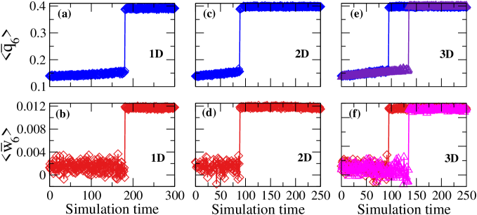
By solving Eq. 8, a new value of is obtained and the algorithm keeps on optimizing this interaction parameter until the goal is reached, i.e., and . The path of the parameters is shown in Fig. 3(a,b) in the and planes. In both, the optimizer correctly tunes to reach the bcc structure which can also be verified by examining the evolution of the average and values as the simulation proceeds. In Fig. 4(a,b), we plot the average and values as a function of the simulation time. At the very beginning of the simulation, and values show that the system is in the fluid phase and as the algorithm optimizes the interactions, there is a sharp transition in both of these values which exactly happens at the fluid-bcc phase boundary. Once the system reaches the bcc phase, it remains in the bcc phase. We also find that as the system reaches the phase boundaries, there is a sudden change in the slope of the parameter’s trajectory as shown in Fig. 3 (c). In other words, the optimizer (Eq. 4) correctly recognizes the phase boundaries present in the phase diagram.

We now analyze the case in which we tune two parameters simultaneously (2 case), the inverse Debye screening length and the pressure of the interaction potential (Eq. 1) while is kept constant. Here, we initialize the system again in the fluid phase at and . The equations of motion (Eq. 4) for the two parameters become
| (9) |
In Fig. 5(a,b), we show the path of the parameters in the and planes. As the simulation time proceeds, SP-ID successfully optimizes both the interaction parameters in such a way that the final structure formed is the bcc crystal. The form of the quality function is the same as we have used for the one parameter case. Variations of and values also verify the formation of the bcc structure from the fluid phase (Fig. 4(c,d)). We find from Fig. 5(c) that the optimizer recognizes the phase boundaries very well as also found for the one parameter case.

Finally, we investigate the case in which we tune three parameters simultaneously (3 case), the inverse Debye screening length , the pressure and the contact value of the interaction potential (Eq. 1). We perform two independent simulations by initializing the system at two different state points in the fluid phase at (i) , and , (ii) , and and optimize all three parameters, , and for the bcc phase. The equations of motion (Eq. 4) when three parameters are tuned become
| (10) |
In Fig. 6, we plot the path of the tuned parameter trajectories as a function of simulation time when the system is initialized in the fluid phase and the desired goal is to reach the targeted bcc structure. Initially, all three parameter values decrease while the system is in the fluid phase and once it crosses the phase boundary between the fluid and bcc phase, they start to saturate.
As the simulation time proceeds, the optimizer successfully optimizes the parameters in such a way that the final structure becomes the bcc phase. Here we also use the same form of the quality function as we have used earlier for the one and two parameter cases.
In Table 1, we show the state point values from which the optimization starts, which correspond to a fluid phase, as well as the final state point obtained from the optimization algorithm, which corresponds to the bcc phase. Note that the parameter values of the pressure and screening length are different as compared to the one- and two-parameter cases, because the contact value is also being optimized.
|
0.4 | 33.0 | 8.0 | ||
|
0.13 | 20.0 | 6.5 |
To confirm that the final structure is a bcc phase, we also plot the evolution of and as a function of the simulation time in Fig. 4(e,f), which indeed confirms that the simulation reaches the optimal bond order parameter values for the bcc phase.
IV.2 Tuning parameters with the CMA-ES method
We now employ the CMA-ES algorithm to analyze all the cases already studied using the SP-ID method, i.e. the tuning of one, two and three parameters, highlighting the differences between the two inverse design optimizers. We use the parameters corresponding to the initial state point employed in the SP-ID algorithm as the initial mean vectors of the multivariate Gaussian distribution in the CMA-ES algorithm. In addition, we start the CMA-ES algorithm with a diagonal covariance matrix with a standard deviation of 10% around its mean value for each parameter. Finally, the initial values of each component of the vectors and are set to zero.
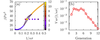
In Fig. 7 we show the results for the one parameter case. The points displayed in Fig 7(a) represent the mean value of the Gaussian distribution in each generation. At the beginning, the algorithm tries to decrease the fitness function value by decreasing the inverse Debye screening length . Since all the steps point in the same direction, the variance of the Gaussian distribution increases (Fig 7(b)) and the mean value overtakes the bcc region, ending up in the fcc phase. After this, the algorithm recognizes the right direction, and the subsequent update is in the opposite direction, i.e. the inverse Debye screening length increases. At the same time, the covariance starts to shrink and the mean value of the Gaussian distribution is found in the bcc region for the first time at the generation. From this generation onwards the updates are in random directions inside the bcc region, leading to a further exponential decrease of the covariance of the Gaussian distribution. At the generation, all the 10 simulations have a value for which the structure corresponds to the stable bcc phase.
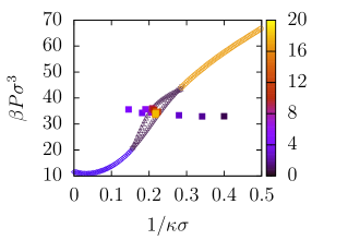

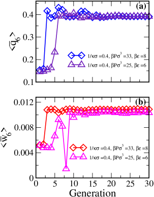
The cases in which we tune two or three parameters do not present significantly different behaviour of the CMA-ES algorithm with respect to the one parameter case. In the two parameter case, enters the bcc region for the first time at the generation, while at the generation all the samples have entered the bcc region, showing how CMA-ES is adversely affected by the dimensionality of the parameter space. The results for the 2 case are shown in Fig 8. We note that the risk of overshooting is lower when more parameters are varied at the same time, since they all contribute to the increase or decrease of the quality function, and the updates of the mean values of the multivariate Gaussian distribution may therefore not always be in the same direction. This prevents the covariance matrix from growing too fast as already shown. Finally, the results for both the investigated 3 cases are shown in Fig 9. We stress that, when varies, the only way to know if we are inside the bcc region is to plot the bond order parameters and check their values, as we show in Fig 10.
These analyses provide benchmarks for how fast the CMS-ES algorithm converges in finding the target structure, as compared to the SP-ID algorithm. Since each generation of the CMA-ES requires times (10 in this work) the computational effort of SP-ID, a comparison of run lengths in the two methods reveals that their efficiencies are very similar. However, in SP-ID, one has information on when the phase boundary is crossed. In CMA-ES the size of the steps from one generation to the other varies, depending on the current form of the covariance matrix. This makes the algorithm explore the landscape in an optimal way, sacrificing information about the phase boundaries. Thus, we conclude that SP-ID and CMA-ES are comparable in their performance, but SP-ID has an edge in retrieving information on the phase boundaries.
V Conclusions
We studied the inverse problem of tuning interaction parameters between charged colloids interacting via a hard-core repulsive Yukawa potential, so that they self-assemble into a targeted crystal structure. We targeted the bcc structure which occupies a narrow region in the phase diagram of the above system and is therefore challenging to find. We showed a comparison between two different optimization algorithms in order to achieve our goal: Statistical Physics-inspired Inverse Design (SP-ID) and Covariance Matrix Adaption - Evolutionary Strategy (CMA-ES). The first makes use of the statistical fluctuations in the bond order parameters to iteratively change the interaction parameters of the system. In addition to effectively tuning the interaction parameters for obtaining the target structure, the SP-ID method correctly identifies the fluid-solid phase boundaries present in the phase diagram. The CMA-ES algorithm generates samples from a multivariate Gaussian distribution at each generation and evaluates the fitness of these samples in order to evolve the interaction parameters of the distribution. The number of generations needed to reach the goal is on average lower in the case of the CMA-ES, and the steps in parameter space are usually larger. This advantage is offset by the need to simulate multiple samples, and we find that the computational effort required in the two methods is comparable. On the other hand, because of the larger step sizes of the parameters, probing phase equilibrium with CMA-ES can be less straightforward than with SP-ID. Most importantly, we showed that both of these inverse methods lead to the targeted bcc structure by tuning the interactions between the particles. Thus, our results demonstrate both methods to be effective search algorithms that may be employed in other design tasks. Although the quality function used here is strictly structural, one may in principle also include quantifiers of dynamics, which may be useful in optimizing the kinetic self-assembly pathways, for example, to account for and exclude glassy dynamics, as well as other kinetic factors of self assembly.
Acknowledgements.
We gratefully acknowledge the India-Netherlands (DST-NWO) joint project grant for supporting the collaboration between the authors.References
- (1) M. Z. Miskin, G. Khaira, J. J. de Pablo, and H. M. Jaeger, PNAS 113, 34 (2016).
- (2) M. C. Rechtsman, F. H. Stillinger, and S. Torquato, Phys. Rev. Lett. 228301, 95 (2005).
- (3) M. C. Rechtsman, F. H. Stillinger, and S. Torquato, Phys. Rev. Lett. 97, 239901 (2006).
- (4) M. C. Rechtsman et al., Phys. Rev. Lett. 101, 073902 (2008).
- (5) M. C. Rechtsman, F. H. Stillinger, and S. Torquato, Phys. Rev. Lett. 101, 085501 (2008).
- (6) S. Torquato, Soft Matter 5, 1157 (2009).
- (7) A. Jain, J. A. Bollinger, and T. M. Truskett, Chem. Eng. J. 60, 2732 (2014).
- (8) J. M. Jaeger, Soft Matter 11, 12 (2015).
- (9) K. M. Ho, C. T. Chan, and C. M. SouKoulis, Phys. Rev. Lett. 65, 3152 (1990).
- (10) A. R. Oganov and C. W. Glass, J. Chem. Phys. 124, 244704 (2006).
- (11) B. I. Dahiyat and S. L. Mayo, Science 278, 82 (1997).
- (12) B. Kuhlman et al., Science 302, 1364 (2003).
- (13) S. Hyun and S. Torquato, J. Mater. Res. 16, 280 (2001).
- (14) A. F. Hannon et al., ACS Macro Lett. 2, 251 (2013).
- (15) J. B. Chang et al., Nat. Commun. 5, 3305 (2014).
- (16) M. C. Rechtsman, F. H. Stillinger, and S. Torquato, Phys. Rev. E 73, 011406 (2006).
- (17) A. F. Hannon et al., Nano Lett. 14, 318 (2014).
- (18) S. Hormoz and M. P. Brenner, PNAS 108, 5193 (2011).
- (19) P. J. Steinhardt, D. R. Nelson, and M. Ronchetti, Phys. Rev. B 28, 784 (1983).
- (20) W. Lechner and C. Dellago, J. Chem. Phys. 129, 114707 (2008).
- (21) S. Kirkpatrick, C. D. Gelatt, and M. P. Vecchi, science 220, 671 (1983).
- (22) L. Ingber, Global optimization C-code, Caltech Alumni Association, Pasadena, CA (1993).
- (23) L. Ingber, arXiv preprint cs/0001018 (2000).
- (24) M. A. M. De Oca, T. Stützle, M. Birattari, and M. Dorigo, in International Workshop on Ant Colony Optimization and Swarm Intelligence, Springer (PUBLISHER, 2006), pp. 1–12.
- (25) M. Mitchell, An introduction to genetic algorithms (MIT press, 1998).
- (26) N. Hansen and A. Ostermeier, Evolutionary computation 9, 159 (2001).
- (27) N. Hansen, S. D. Müller, and P. Koumoutsakos, Evolutionary computation 11, 1 (2003).
- (28) N. Hansen, Towards a new evolutionary computation (Springer, 2006), pp. 75–102.
- (29) E. J. Meijer and F. El Azhar, F.El Azhar, J. Chem. Phys. 106, 4678 (1997).
- (30) F. El Azhar, M. Baus, J. P. Ryckaert, and E. J. Meijer, J. Chem. Phys. 112, 5121 (2000).
- (31) A. P. Hynninen and M. Dijkstra, Phys. Rev. E 68, 021407 (2003).
- (32) J. A. van Meel, L. Filion, C. Valeriani, and D. Frenkel, J. Chem. Phys. 136, 234107 (2012).