A Geometric Modeling of Occam’s Razor in Deep Learning

Abstract

Why do deep neural networks (DNNs) benefit from very high dimensional parameter spaces? Their huge parameter complexities vs. stunning performances in practice is all the more intriguing and not explainable using the standard theory of regular models. In this work, we propose a geometrically flavored information-theoretic approach to study this phenomenon. Namely, we introduce the locally varying dimensionality of the parameter space of neural network models by considering the number of significant dimensions of the Fisher information matrix, and model the parameter space as a manifold using the framework of singular semi-Riemannian geometry. We derive model complexity measures which yield short description lengths for deep neural network models based on their singularity analysis thus explaining the good performance of DNNs despite their large number of parameters.

1 Introduction

Deep neural networks (DNNs) are usually large models in terms of storage costs. In the classical model selection theory, such models are not favored as compared to simple models with the same training performance. For example, if one applies the Bayesian information criterion (BIC) [61] to DNN, a shallow neural network (NN) will be preferred over a deep NN due to the penalty term with respect to (w.r.t.) the complexity. A basic principle in science is the Occam’s Razor, which favors simple models over complex ones that accomplish the same task. This raises the fundamental question of how to measure the simplicity or the complexity of a model.

Formally, the preference of simple models has been studied in the area of minimum description length (MDL) [57, 58, 22], also known in another thread of research as the minimum message length (MML) [67].

Consider a parametric family of distributions $\mathcal{M}=\{p(\bm{x}\,|\,\bm{\theta})\}$ with $\bm{\theta}\in\Theta\subset\mathbb{R}^{D}$. The distributions are mutually absolutely continuous, which guarantees all densities to have the same support. Otherwise, many problems of non-regularity will arise as described by [24, 53]. The Fisher information matrix (FIM) $\mathcal{I}(\bm{\theta})$ is a $D\times{D}$ positive semi-definite (psd) matrix: $\mathcal{I}(\bm{\theta})\succeq 0$. The model is called regular if it is (i) identifiable [11] with (ii) a non-degenerate and finite Fisher information matrix (i.e., $\mathcal{I}(\bm{\theta})\succ 0$).

In a Bayesian setting, the description length of a set of $N$ i.i.d. observations $\bm{X}=\{\bm{x}_{i}\}_{i=1}^{N}\subset\mathcal{X}$ w.r.t. $\mathcal{M}$ can be defined as the number of nats with the coding scheme of a parametric model $p(\bm{x}\,|\,\bm{\theta})$ and a prior $p(\bm{\theta})$. The code length of any $\bm{x}_{i}$ is given by the cross entropy between the empirical distribution $\delta_{i}(\bm{x})=\delta(\bm{x}-\bm{x}_{i})$, where $\delta(\cdot)$ denotes the Dirac’s delta function, and $p(\bm{x})=\int p(\bm{x}\mid\bm{\theta})p(\bm{\theta})\,\mathrm{d}\bm{\theta}$. Therefore, the description length of $\bm{X}$ is

$$-\log p(\bm{X})=\sum_{i=1}^{N}h^{\times}(\delta_{i}:p)=-\sum_{i=1}^{N}\log\int p(\bm{x}_{i}\mid\bm{\theta})\,p(\bm{\theta})\,\mathrm{d}\bm{\theta},$$ (1)

where $h^{\times}(p:q)\vcentcolon=-\int p(\bm{x})\log q(\bm{x})\mathrm{d}\bm{x}$ denotes the cross entropy between $p(\bm{x})$ and $q(\bm{x})$.

By using Jeffreys’ non-informative prior [3] as $p(\bm{\theta})$, the MDL in eq. 1 can be approximated (see [57, 58, 7]) as

$$\chi=\underbrace{-\log p(\bm{X}\,|\,\hat{\bm{\theta}})}_{\mbox{fitness}}+\overbrace{\underbrace{\frac{D}{2}\log\frac{N}{2\pi}}_{\mbox{penalize high dof}}+\underbrace{\log\left(\int\sqrt{|\mathcal{I}(\bm{\theta})|}\;d\bm{\theta}\right)}_{\mbox{model capacity}}}^{\mbox{geometric complexity}}.$$ (2)

where $\hat{\bm{\theta}}\in\Theta$ is the maximum likelihood estimation (MLE), or the projection [3] of $\bm{X}$ onto the model, $D=\dim(\Theta)$ is the model size, $N$ is the number of observations, and $|\cdot|$ denotes the matrix determinant. In this paper, the symbols $\chi$ and $\mathcal{O}$ and the term “razor” all refer to the same concept, that is the description length of the data $\bm{X}$ by the model $\mathcal{M}$. The smaller those quantities, the better.

The first term in eq. 2 is the fitness of the model to the observed data. The second and the third terms measures the geometric complexity [43] and make $\chi$ favor simple models. The second $O(\log{N})$ term only depends on the number of parameters $D$ and the number of observations $N$. It penalizes large models with a high degree of freedom (dof). The third $O(1)$ term is independent to the observed data and measures the model capacity, or the total “number” of distinguishable distributions [43] in the model.

Unfortunately, this razor $\chi$ in eq. 2 does not fit straightforwardly into DNNs, which are high-dimensional singular models. The FIM $\mathcal{I}(\bm{\theta})$ are large singular matrices (not full rank) and the last term may be difficult to evaluate. Based on the second term on the right-hand-side (RHS), a DNN can have very high complexity and therefore is less favored against a shallow network. This contradicts the good generalization of DNNs as compared to shallow NNs. These issues call for a new analysis of the MDL in the DNN setting.

Towards this direction, we made the following contributions in this paper:

• New concepts and methodologies from singular semi-Riemannian geometry [36] to analyze the space of neural networks;

• A definition of the local dimensionality, that is the amount of non-singularity, with bounding analysis;

• A new MDL formulation, which explains how the singularity contribute to the “negative complexity” of DNNs: That is, the model turns simpler as the number of parameters grows.

The rest of this paper is organized as follows. Section 2 reviews singularities in information geometry. In the setting of a DNN, section 3 introduces its singular parameter manifold, and bound the number of singular dimensions. Sections 4, 5, 6 and 7 derive our MDL criterion based on two different priors, and discusses how model complexity is affected by the singular geometry. We discuss related work in section 8 and conclude in section 9.

2 Lightlike Statistical Manifold

In this paper, bold capital letters like $\bm{A}$ denote matrices, bold small letters like $\bm{a}$ denote vectors, and normal capital/small letters like $A$/$a$ and Greek letters like $\alpha$ denote scalars (with exceptions).

The term “statistical manifold” refers to $\mathcal{M}=\left\{p(\bm{x}\,|\,\bm{\theta})\right\}$, where each point of $\mathcal{M}$ corresponds to a probability distribution $p(\bm{x}\,|\,\bm{\theta})$. The discipline of information geometry [3] studies such a space in the Riemannian and more generally differential geometry framework. Hotelling [26] and independently Rao [55, 56] proposed to endow a parametric space of statistical models with the Fisher information matrix as a Riemannian metric:

$$\mathcal{I}(\bm{\theta})\vcentcolon=\mathbb{E}_{p}\left(\frac{\partial\log p(\bm{x}\,|\,\bm{\theta})}{\partial\bm{\theta}}\frac{\partial\log p(\bm{x}\,|\,\bm{\theta})}{\partial\bm{\theta}^{\intercal}}\right),$$ (3)

where $\mathbb{E}_{p}$ denotes the expectation w.r.t. $p(\bm{x}\,|\,\bm{\theta})$. The corresponding infinitesimal squared length element $\mathrm{d}s^{2}=\mathrm{tr}(\mathcal{I}(\bm{\theta})d\bm{\theta}d\bm{\theta}^{\intercal})=\langle d\bm{\theta},d\bm{\theta}\rangle_{\mathcal{I}(\bm{\theta})}=d\bm{\theta}^{\intercal}\mathcal{I}(\bm{\theta})d\bm{\theta}$, where $\mathrm{tr}(\cdot)$ means the matrix trace, is independent of the underlying parameterization of the population space.

Amari further developed this approach by revealing the dualistic structure of statistical manifolds which extends the Riemannian framework [3, 47]. The MDL criterion arising from the geometry of Bayesian inference with Jeffreys’ prior for regular models is detailed in [7]. In information geometry, the regular assumption is (1) an open connected parameter space in some Euclidean space; and (2) the FIM exists and is non-singular. However, in general, the FIM is only positive semi-definite and thus for non-regular models like neuromanifolds [3] or Gaussian mixture models [68], the manifold is not Riemannian but singular semi-Riemannian [36, 15]. In the machine learning community, singularities have often been dealt with as a minor issue: For example, the natural gradient has been generalized based on the Moore-Penrose inverse of $\mathcal{I}(\bm{\theta})$ [65] to avoid potential non-invertible FIMs. Watanabe [68] addressed the fact that most usual learning machines are singular in his singular learning theory which relies on algebraic geometry. Nakajima and Ohmoto [45] discussed dually flat structures for singular models.

Recently, preliminary efforts [6, 28] tackle singularity at the core, mostly from a mathematical standpoint. For example, Jain et al. [28] studied the Ricci curvature tensor of such manifolds. These mathematical notions are used in the community of differential geometry or general relativity but have not yet been ported to the machine learning community.

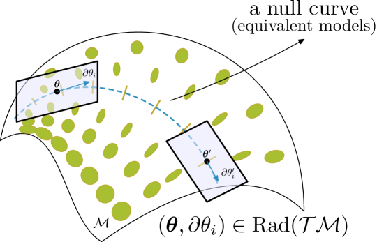
Figure 1: A toy lightlike manifold $\mathcal{M}$ with a null curve. The ellipses are Tissot’s indicatrices, showing how circles of infinitesimal radius are distorted by the lightlike geometry on $\mathcal{M}$. On the null curve, the FIM is degenerate so that $\langle\partial\theta_{i},\partial\theta_{i}\rangle_{\mathcal{I}}=0$. Therefore the local dynamic $\partial\theta_{i}$ (tangent vector of the null curve) has zero length, meaning that it does not change the model. The radical distribution $\mathrm{Rad}(\mathcal{TM})$ is formed by the null curve and its tangent vectors.

Following these efforts, we first introduce informally some basic concepts from a machine learning perspective to define the differential geometry of non-regular statistical manifolds. The tangent space $\mathcal{T}_{\bm{\theta}}(\mathcal{M})$ is a $D$-dimensional ($D=\dim(\mathcal{M})$) real vector space, that is the local linear approximation of the manifold $\mathcal{M}$ at the point $\bm{\theta}\in\mathcal{M}$, equipped with the inner product induced by $\mathcal{I}(\bm{\theta})$. The tangent bundle $\mathcal{TM}\vcentcolon=\{({\bm{\theta}},\bm{v}),\bm{\theta}\in\mathcal{M},\bm{v}\in\mathcal{T}_{\bm{\theta}}\}$ is the $2D$-dimensional manifold obtained by combining all tangent spaces for all $\bm{\theta}\in\mathcal{M}$. A vector field is a smooth mapping from $\mathcal{M}$ to $\mathcal{TM}$ such that each point $\bm{\theta}\in\mathcal{M}$ is attached a tangent vector originating from itself. Vector fields are cross-sections of the tangent bundle. In a local coordinate chart $\bm{\theta}$, the vector fields along the frame are denoted as $\partial\theta_{i}$. A distribution (not to be confused with probability distributions which are points on $\mathcal{M}$) means a vector subspace of the tangent bundle spanned by several independent vector fields, such that each point $\bm{\theta}\in\mathcal{M}$ is associated with a subspace of $\mathcal{T}_{\bm{\theta}}(\mathcal{M})$ and those subspaces vary smoothly with $\bm{\theta}$. Its dimensionality is defined by the dimensionality of the subspace, i.e., the number of vector fields that span the distribution.

In a lightlike manifold [36, 15] $\mathcal{M}$, $\mathcal{I}(\bm{\theta})$ can be degenerate. The tangent space $\mathcal{T}_{\bm{\theta}}(\mathcal{M})$ is a vector space with a kernel subspace, i.e., a nullspace. A null vector field is formed by null vectors, whose lengths measured according to the Fisher metric tensor are all zero. The radical distribution $\mathrm{Rad}(\mathcal{TM})$ is the distribution spanned by the null vector fields. Locally at $\bm{\theta}\in\mathcal{M}$, the tangent vectors in $\mathcal{T}_{\bm{\theta}}(\mathcal{M})$ which span the kernel of $\mathcal{I}(\bm{\theta})$ are denoted as $\mathrm{Rad}_{\bm{\theta}}(\mathcal{TM})$. In a local coordinate chart, $\mathrm{Rad}(\mathcal{TM})$ is well defined if these $\mathrm{Rad}_{\bm{\theta}}(\mathcal{TM})$ form a valid distribution. We write $\mathcal{TM}=\mathrm{Rad}(\mathcal{TM})\oplus\mathcal{S}(\mathcal{TM})$, where ‘$\oplus$” is the direct sum, and the screen distribution $\mathcal{S}(\mathcal{TM})$ is complementary to the radical distribution $\mathrm{Rad}(\mathcal{TM})$ and has a non-degenerate induced metric. See fig. 1 for an illustration of the concept of radical distribution.

We can find a local coordinate frame (a frame is an ordered basis) $\left(\theta_{1},\cdots,\theta_{d},\theta_{d+1},\cdots,\theta_{D}\right)$, where the first $d$ dimensions $\bm{\theta}^{s}=(\theta_{1},\cdots,\theta_{d})$ correspond to the screen distribution, and the remaining $\bar{d}\vcentcolon={}D-d$ dimensions $\bm{\theta}^{r}=(\theta_{d+1},\cdots,\theta_{D})$ correspond to the radical distribution. The local inner product $\langle\cdot,\cdot\rangle_{\mathcal{I}}$ satisfies

$$\langle\partial\theta_{i},\partial\theta_{j}\rangle_{\mathcal{I}} =\delta_{ij},\quad(\forall\ {1}\leq{i,j}\leq{d})$$

$$\langle\partial\theta_{i},\partial\theta_{k}\rangle_{\mathcal{I}} =0,\quad(\forall\ {d+1}\leq{i}\leq{}D,\;1\leq{k}\leq{D})$$

where $\delta_{ij}=1$ if and only if (iff) $i=j$ and $\delta_{ij}=0$, otherwise. Unfortunately, this frame is not unique [14]. We will abuse $\mathcal{I}$ to denote both the FIM of $\bm{\theta}$ and the FIM of $\bm{\theta}^{s}$. One has to remember that $\mathcal{I}(\bm{\theta})\succeq 0$, while $\mathcal{I}(\bm{\theta}^{s})\succ 0$ is a proper Riemannian metric. Hence, both $\mathcal{I}^{-1}(\bm{\theta}^{s})$ and $\log|\mathcal{I}(\bm{\theta}^{s})|$ are well-defined.

3 Local Dimensionality

This section instantiates the concepts in the previous section 2 in terms of a simple DNN structure. We consider a deep feed-forward network with $L$ layers, uniform width $M$ except the last layer which has $m$ output units ($m<M$), input $\bm{z}\in\mathcal{Z}$ with $\dim(\mathcal{Z})=M$, pre-activations $\bm{h}^{l}$ of size $M$ (except that in the last layer, $\bm{h}^{L}$ has $m$ elements), post-activations $\bm{z}^{l}$ of size $M$, weight matrices $\bm{W}^{l}$ and bias vectors $\bm{b}^{l}$ ($1\leq{l}\leq{L}$). The layers are given by

$$\bm{z}^{l} =\phi(\bm{h}^{l}),$$ (4)

$$\bm{h}^{l} =\bm{W}^{l}\bm{z}^{l-1}+\bm{b}^{l},$$

$$\bm{z}^{0} =\bm{z},$$

where $\phi$ is an element-wise nonlinear activation function such as ReLU [19].

Without loss of generality, we assume multinomial output units and the DNN output [20]

$$y\sim\mathrm{Multinomial}\left(\mathrm{SoftMax}(\bm{h}^{L})\right)$$

is a random label in the set $\{1,\cdots,m\}$, where

$$\mathrm{SoftMax}(\bm{t})\vcentcolon=\frac{1}{\sum_{i=1}^{m}\exp(t_{i})}\left(\exp(t_{1}),\exp(t_{2}),\cdots,\exp(t_{m})\right)$$

denotes the softmax function. $\mathrm{SoftMax}(\bm{h}^{L})$ is a random point in $\Delta^{m}$, the $(m-1)$ dimensional statistical simplex. Therefore, $p(y=k)=\exp(h^{L}_{k})/{\sum_{j=1}^{m}\exp(h^{L}_{j})}$, $k=1,\cdots,m$. An observation $\bm{x}=(\bm{z},y)$ consists of both the input $\bm{z}$ and the target $y$. The joint probability distribution has the form

$$\log p(\bm{X}\,|\,\bm{\theta})=\log p(\bm{Z})+\sum_{i=1}^{N}\log p({y}_{i}\,|\,\bm{z}_{i},\,\bm{\theta}),$$

where $\bm{\theta}$ consists of all neural network parameters including $\bm{W}^{l}$ and $\bm{b}^{l}$, $l=1,\cdots,L$, and $p(\bm{Z})$ by assumption is parameter free. Notice that we use $\bm{X}$ and $\bm{Z}$ to denote a collection of $N$ random observations and use $\bm{x}$ and $\bm{z}$ to denote one single observation. Our results can be generalized to similar models including stochastic neural networks [10].

All such neural networks $\mathrm{NN}_{\bm{\theta}}$ when $\bm{\theta}$ varies in a parameter space are referred to as the neuromanifold: $\mathcal{M}=\{\mathrm{NN}_{\bm{\theta}}:\;{\bm{\theta}\in\Theta}\}$, where $\mathcal{M}$ is abused to denote both a general statistical manifold in section 2 and a neuromanifold. In machine learning, we are often interested in the FIM w.r.t. $\bm{\theta}$ as it reveals the geometry of the parameter space. However, by definition, the FIM can also be computed relatively w.r.t. a subset of $\bm{\theta}$ in a sub-system [63]. In this paper, we are concerned with the single-observation FIM (see e.g. [49][62] for derivations)

$$\mathcal{I}(\bm{\theta}) =\frac{1}{N}\sum_{i=1}^{N}\left[\left(\frac{\partial\bm{h}^{L}(\bm{z}_{i})}{\partial\bm{\theta}}\right)^{\intercal}\bm{C}_{i}\frac{\partial\bm{h}^{L}(\bm{z}_{i})}{\partial\bm{\theta}}\right],$$ (5)

where $\frac{\partial\bm{h}^{L}(\bm{z}_{i})}{\partial\bm{\theta}}$ is the $m\times{D}$ parameter-output Jacobian matrix, based on a given input $\bm{z}_{i}$, $\bm{C}_{i}\vcentcolon=\mathrm{diag}\left({\bm{o}_{i}}\right)-\bm{o}_{i}\bm{o}_{i}^{\intercal}\succ 0$, $\mathrm{diag}\left({\cdot}\right)$ means the diagonal matrix with the given diagonal entries, and $\bm{o}_{i}\vcentcolon=\mathrm{SoftMax}(\bm{h}^{L}(\bm{z}_{i}))$ is the predicted class probabilities of the $i$’th sample. It is obvious that the FIM w.r.t. the joint distribution $p(\bm{X}\,|\,\bm{\theta})$ of multiple observations is $N\mathcal{I}(\bm{\theta})$ (Fisher information is additive), so that $\mathcal{I}(\bm{\theta})$ does not scale with $N$.

By considering the neural network weights and biases as random variables satisfying a prescribed prior distribution [30, 52], this $\mathcal{I}(\bm{\theta})$ can be regarded as a random matrix [42] depending on the structure of the DNN and the prior. The empirical density of $\mathcal{I}(\bm{\theta})$ is the empirical distribution of its eigenvalues $\{\lambda_{i}\}_{i=1}^{D}$, that is, $\rho_{D}(\lambda)=\frac{1}{D}\sum_{i=1}^{D}\delta(\lambda_{i})$. If at the limit $D\to\infty$, the empirical density converges to a probability density function (pdf)

$$\rho_{\mathcal{I}}(\lambda)\vcentcolon=\lim_{D\to\infty}\rho_{D}(\lambda)$$ (6)

called the spectral density of the Fisher information matrix.

Definition 1 (Local dimensionality).

The local dimensionality $d(\bm{\theta})\vcentcolon=\mathrm{rank}\left({\mathcal{I}(\bm{\theta})}\right)$ of the neuromanifold $\mathcal{M}$ at $\bm{\theta}\in\mathcal{M}$ refers to the rank of the FIM $\mathcal{I}(\bm{\theta})$.

The local dimensionality $d(\bm{\theta})$ is the number of degrees of freedom at $\bm{\theta}\in\mathcal{M}$ which can change the probabilistic model $p(y\,|\,\bm{z},\bm{\theta})$ in terms of information theory. One can find a reparametrization with $d(\bm{\theta})$ parameters, which is locally equivalent to the original DNN with $D$ parameters. Recall the dimensionality of the tangent bundle is two times the dimensionality of the manifold.

Remark 1.

The dimensionality of the screen distribution $\mathcal{S}(\mathcal{TM})$ at $\bm{\theta}$ is $2\,d(\bm{\theta})$.

By definition, the FIM as the singular semi-Riemannian metric of $\mathcal{M}$ must be psd. Therefore it only has positive and zero eigenvalues, and the number of positive eigenvalues $d(\bm{\theta})$ is not constant as ${\bm{\theta}}$ varies in general.

Remark 2.

The local metric signature (number of positive, negative, zero eigenvalues of the FIM) of the neuromanifold $\mathcal{M}$ is $\left(d(\bm{\theta}),0,D-d(\bm{\theta})\right)$, where $d(\bm{\theta})$ is the local dimensionality.

For DNN, we can safely assume that

(A1)

At the MLE $\hat{\bm{\theta}}$, the prediction $\mathrm{SoftMax}(\bm{h}^{L}(\bm{z}_{i}))$ perfectly recovers (tending to be one-hot vectors) the training target $y_{i}$, for all the training samples $(\bm{z}_{i},y_{i})$.

In this case, the negative Hessian of the average log-likelihood

$$\mathfrak{J}(\bm{\theta})\vcentcolon=-\frac{1}{N}\frac{\partial^{2}\log p(\bm{X}\,|\,\bm{\theta})}{\partial\bm{\theta}\partial\bm{\theta}^{\intercal}}=-\frac{1}{N}\sum_{i=1}^{N}\frac{\partial^{2}\log p(y_{i}\,|\,\bm{z}_{i},\bm{\theta})}{\partial\bm{\theta}\partial\bm{\theta}^{\intercal}}$$

is called the observed FIM (sample-based FIM) and coincides with the FIM at the MLE and $\mathfrak{J}(\hat{\bm{\theta}})=\mathcal{I}(\hat{\bm{\theta}})$. For general statistical models, there is a residual term in between these two matrices which scales with the training error (see e.g. Eq. 6.19 in section 6 of [4], or eq. 17 in the appendix). One can use the rank of the negative Hessian $\mathfrak{J}(\bm{\theta})$ (i.e., observed rank) to get an approximation $\hat{d}(\bm{\theta})\vcentcolon=\mathrm{rank}\left({\mathfrak{J}(\bm{\theta})}\right)$ of the local dimensionality $d(\bm{\theta})$. In the MLE $\hat{\bm{\theta}}$, the approximation becomes accurate. We simply denote $d$ and $\hat{d}$, instead of $d(\bm{\theta})$ and $\hat{d}(\bm{\theta})$, if $\bm{\theta}$ is clear from the context.

We first show that the lightlike dimensions of $\mathcal{M}$ do not affect the neural network model in eq. 4.

Lemma 1.

If $(\bm{\theta},\sum_{j}\alpha_{j}\partial\theta_{j})\in\mathrm{Rad}(\mathcal{TM})$, i.e. $\langle\sum_{j}\alpha_{j}\partial\theta_{j},\sum_{j}\alpha_{j}\partial\theta_{j}\rangle_{\mathcal{I}(\bm{\theta})}=0$, then $\forall{i}=1\cdots{N}$, $\frac{\partial\bm{h}^{L}(\bm{z}_{i})}{\partial\bm{\theta}}\bm{\alpha}=\lambda_{i}\bm{1}$, where $\lambda_{i}\in\mathbb{R}$, and $\bm{1}$ is a vector of ones.

By lemma 1, the Jacobian $\frac{\partial\bm{h}^{L}(\bm{z}_{i})}{\partial\bm{\theta}}$ is the local linear approximation of the map $\bm{\theta}\to\bm{h}^{L}$. The dynamic $\bm{\alpha}$ (coordinates of a tangent vector) on $\mathcal{M}$ causes a uniform increment on the output $\bm{h}^{L}$, which, after the $\mathrm{SoftMax}$ function, does not change the neural network map $\bm{z}_{i}\to{y}$.

Then, we have the following bounds.

Theorem 2.

$\forall\bm{\theta}\in\mathcal{M}$, $\hat{d}(\bm{\theta})\leq{}d(\bm{\theta})\leq\min(D,(m-1)N)$.

Remark 3.

While the total number $D$ of free parameters is unbounded in DNNs, the local dimensionality $d(\bm{\theta})$ grows at most linearly w.r.t. the sample size $N$, given fixed $m$ (size of the last layer). If both $N$ and $m$ are fixed, then $d(\bm{\theta})$ is bounded even when the network width $M\to\infty$ and/or depth $L\to\infty$.

To understand $\hat{d}(\bm{\theta})\leq{}d(\bm{\theta})$, one can parameterize the DNN, locally, with only $d(\bm{\theta})$ free parameters while maintaining the same predictive model. The log-likelihood is a function of these $d(\bm{\theta})$ parameters, and therefore its Hessian has at most rank $d(\bm{\theta})$. In theory, one can only reparameterize $\mathcal{M}$ so that at one single point $\hat{\bm{\theta}}$, the screen and radical distributions are separated based on the coordinate chart. Such a chart may neither exist locally (in a neighborhood around $\hat{\bm{\theta}}$) nor globally.

The local dimensionality is not constant and may vary with $\bm{\theta}$. The global topology of the neuromanifold is therefore like a stratifold [5, 16]. As $\bm{\theta}$ has a large dimensionality in DNNs, singularities are more likely to occur in $\mathcal{M}$. Compared to the notion of intrinsic dimensionality [38], our $d(\bm{\theta})$ is well-defined mathematically rather than based on empirical evaluations. One can regard our local dimensionality as an upper bound of the intrinsic dimensionality, because a very small singular value of $\mathcal{I}$ still counts towards the local dimensionality. Notice that random matrices have full rank with probability 1 [17]. On the other hand, if we regard small singular values (below a prescribed threshold $\varepsilon>0$) as $\varepsilon$-singular dimensions, the spectral density $\rho_{\mathcal{I}}$ (probability distribution of the eigenvalues of $\mathcal{I}(\bm{\theta})$) affects the expected local dimensionality of $\mathcal{M}$. If the pdf $\rho_{\mathcal{I}}$ is “flat” (close to uniform), $\mathcal{M}$ is less likely to be singular; if $\rho_{\mathcal{I}}$ is “spiky”, $\mathcal{M}$ is likely to have a small local dimensionality. By the Cramér-Rao lower bound, the variance of an unbiased 1D estimator $\hat{\theta}$ must satisfy

$$\mathrm{var}(\hat{\theta})\geq\mathcal{I}(\theta)^{-1}\geq\frac{1}{\varepsilon}.$$

Therefore the $\varepsilon$-singular dimensions lead to a large variance of the estimator $\hat{\theta}$: a single observation $\bm{x}_{i}$ carries little or no information regarding $\theta$, and it requires a large number of observations to achieve the same precision.

In a DNN, there are several typical sources of singularities:

• First, if the neuron is saturated and gives constant output regardless of the input sample $\bm{z}_{i}$, then all dynamics of its input and output connections are in $\mathrm{Rad}(\mathcal{TM})$.

• Second, two neurons in the same layer can have linearly dependent output, e.g. when they share the same weight vector and bias. They can be merged into one single neuron, as there exists redundancy in the original reparametrization.

• Third, if the activation function $\phi(\cdot)$ is homogeneous, e.g. ReLU, then any neuron in the DNN induces a reparametrization by multiplying the input links by $\alpha$ and output links by $1/\alpha^{k}$ ($k$ is the degree of homogeneity). This reparametrization corresponds to a null curve in the neuromanifold parameterized by $\alpha$.

• Fourth, certain structures such as recurrent neural networks (RNNs) suffer from vanishing gradient [20]. As the FIM is the variance of the gradient of the log-likelihood (known as variance of the score in statistics), its scale goes to zero along the dimensions associated with such structures.

In the neural network model, all parameters in the $l$’th layer consist of the weights $\bm{W}^{l}$ and the bias $\bm{b}^{l}$. The submanifold obtained by varying only these parameters with all other parameters fixed to $\bm{\theta}^{\star}$ is denoted by $\mathcal{M}_{l}(\bm{\theta}^{\star})=\{\mathrm{NN}_{\bm{\theta}}:\,\bm{\theta}\in\Theta;\theta_{i}=\theta^{\star}_{i},\forall{i}\not\in G_{l}\}$, where $G_{l}$ is the index set of the $l$’th layer, which are the indexes of $\bm{\theta}$ associated with the parameters $\bm{W}^{l}$ and $\bm{b}^{l}$. Its metric is a diagonal block of $\mathcal{I}(\bm{\theta})$, denoted by $\mathcal{I}_{l}(\bm{\theta})$. If $(\bm{\theta},\sum_{j}\alpha_{j}\partial\theta_{j})\in\mathrm{Rad}(\mathcal{TM}_{l})$, then $\alpha_{j}=0$, $\forall{j}\not\in G_{l}$, and $\langle\sum_{j}{\alpha}_{j}\partial\theta_{j},\sum_{j}{\alpha}_{j}\partial\theta_{j}\rangle_{\mathcal{I}(\bm{\theta})}=0$. The local dynamic $\sum_{j}\alpha_{j}\partial\theta_{j}$ in the $l$’th layer does not change the global prediction model. This shows that $\mathrm{Rad}(\mathcal{TM}_{l})$ is a submanifold of $\mathrm{Rad}(\mathcal{TM})$. We have the following result on the local dimensionality of the global model and neural network layers.

Theorem 3.

For the neural network model in eq. 4, we have

$$\sum_{l=1}^{L}\dim(\mathrm{Rad}(\mathcal{TM}_{l}))\leq\dim(\mathrm{Rad}(\mathcal{TM})).$$

Based on theorem 3, the number of possible local reparametrization (without changing the neural network model) is smaller than the number of global reparametrization. This is intuitive as there can be non-local parametrizations across different layers without affecting the output (see the third source of singularity above).

To investigate the singularity across different layers, we study the FIM $\mathcal{I}(\bm{z}^{l})$ w.r.t. the intermediate representation $\bm{z}^{l}$ ($1\leq{l}\leq{L-1}$).

Theorem 4.

If $1\leq l_{1}<l_{2}\leq L-1$, then

$$\mathrm{rank}\left({\mathcal{I}(\bm{z}^{l_{1}})}\right)\leq\mathrm{rank}\left({\mathcal{I}(\bm{z}^{l_{2}})}\right).$$

Lower levels in a DNN model (close to the input) have more singularity than higher layers (close to the output). This is intuitive, as neuron dynamics in deeper layers are harder to reach the final output.

It is meaningful to formally define the notion of “lightlike neuromanifold”. Using the geometric tools, related studies can be invariant w.r.t. neural network reparametrization. Moreover, the connection between neuromanifold and singular semi-Riemannian geometry, which is used in general relativity, is not yet widely adopted in machine learning. For example, the textbook [68] in singular statistics mainly used tools from algebraic geometry which is a different field.

Notice that the Fisher-Rao distance along a null curve is undefined because there the FIM is degenerate and there is no arc-length reparameterization along null curves [32].

4 General Formulation of Our Razor

In this section, we derive a new formula of MDL for DNNs, aiming to explain how does the high dimensional DNN structure can have a short code length of the given data? Notice that, this work focuses on the concept of model complexity but not the generalization bounds. We try to argue the DNN model is intrinsically simple because it can be described shortly. The theoretical connection between generalization power and MDL is studied in PAC-Bayesian theory and PAC-MDL (see [21, 46, 25] and references therein). This is beyond the scope of this paper.

We derive a simple asymptotic formula for the case of large sample size and large network size. Therefore crude approximations are taken and the low-order terms are ignored, which are common practices in deriving information criteria [1, 61].

In the following, we will abuse $p(\bm{x}\,|\,\bm{\theta})$ to denote the DNN model $p(y\,|\,\bm{z},\,\bm{\theta})$ for shorter equations and to be consistent with the introduction. Assume

(A2)

The absolute values of the third order derivatives of $\log{p}(\bm{x}\,|\,\bm{\theta})$ w.r.t. $\bm{\theta}$ are bounded by some constant.

(A3)

$\forall{i}$, $|\theta_{i}-\hat{\theta}_{i}|=O(1/\sqrt{M})$, where $O(\cdot)$ is the Bachmann–Landau’s big-O notation.

Recall that $M$ is the width of the neural network. We consider that the neural networks weights have a order of $O(1/\sqrt{M})$. For example, if the input of a neuron follows the standard Gaussian distribution, then its weights with order $O(1/\sqrt{M})$ guarantee the output is $O(1)$. In practice, this constraint can be guaranteed by clipping the weight vector to a prescribed range.

We rewrite the code length in eq. 1 based on the Taylor expansion of $\log{p}(\bm{X}\,|\,\bm{\theta})$ at $\bm{\theta}=\hat{\bm{\theta}}$ up to the second order:

$$-\log p(\bm{X})= -\log\int_{\mathcal{M}}p(\bm{\theta})\exp\bigg{(}\log{p}(\bm{X}\,|\,\hat{\bm{\theta}})-\frac{N}{2}(\bm{\theta}-\hat{\bm{\theta}})^{\intercal}\mathfrak{J}(\hat{\bm{\theta}})(\bm{\theta}-\hat{\bm{\theta}})$$

$$\quad\quad+O\left(N\|\bm{\theta}-\hat{\bm{\theta}}\|^{3}\right)\bigg{)}\mathrm{d}\bm{\theta}.$$ (7)

Notice that the first order term vanishes because $\hat{\bm{\theta}}$ is a local optimum of $\log p(\bm{X}\,|\,\bm{\theta})$, and in the second order term, $-N\mathfrak{J}(\hat{\bm{\theta}})$ is the Hessian matrix of the likelihood function $\log{p}(\bm{X}\,|\,\bm{\theta})$ evaluated at $\hat{\bm{\theta}}$. At the MLE, $\mathfrak{J}(\hat{\bm{\theta}})\succeq 0$, while in general the Hessian of the loss of a DNN evaluated at $\bm{\theta}\neq\hat{\bm{\theta}}$ can have a negative spectrum [2, 59].

Through a change of variable $\bm{\phi}\vcentcolon=\sqrt{N}(\bm{\theta}-\hat{\bm{\theta}})$, the density of $\bm{\phi}$ is $p(\bm{\phi})=\frac{1}{\sqrt{N}}p(\frac{\bm{\phi}}{\sqrt{N}}+\hat{\bm{\theta}})$ so that $\int_{\mathcal{M}}p(\bm{\phi})d\bm{\phi}=1$. In the integration in section 4, the term $-\frac{N}{2}(\bm{\theta}-\hat{\bm{\theta}})^{\intercal}\mathfrak{J}(\hat{\bm{\theta}})(\bm{\theta}-\hat{\bm{\theta}})$ has an order of $O(\|\bm{\phi}\|^{2})$. The cubic remainder term has an order of $O(\frac{1}{\sqrt{N}}\|\bm{\phi}\|^{3})$. If $N$ is sufficiently large, this remainder can be ignored. Therefore we can write

$$-\log{p}(\bm{X}) \approx-\log{p}(\bm{X}\,|\,\hat{\bm{\theta}})-\log\mathbb{E}_{p}\exp\bigg{(}-\frac{N}{2}(\bm{\theta}-\hat{\bm{\theta}})^{\intercal}\mathfrak{J}(\hat{\bm{\theta}})(\bm{\theta}-\hat{\bm{\theta}})\bigg{)}.$$ (8)

On the RHS, the first term measures the error of the model w.r.t. the observed data $\bm{X}$. The second term measures the model complexity. We have the following bound.

Proposition 5.

$$0 \leq{}-\log\mathbb{E}_{p}\exp\bigg{(}-\frac{N}{2}(\bm{\theta}-\hat{\bm{\theta}})^{\intercal}\mathfrak{J}(\hat{\bm{\theta}})(\bm{\theta}-\hat{\bm{\theta}})\bigg{)}$$

$$\leq{}\frac{N}{2}\mathrm{tr}\left(\mathfrak{J}(\hat{\bm{\theta}})\left((\mu(\bm{\theta})-\hat{\bm{\theta}})(\mu(\bm{\theta})-\hat{\bm{\theta}})^{\intercal}+\mathrm{cov}(\bm{\theta})\right)\right),$$

where $\mu(\bm{\theta})$ and $\mathrm{cov}(\bm{\theta})$ denote the mean and covariance matrix of the prior $p(\bm{\theta})$, respectively.

Therefore the complexity is always non-negative and its scale is bounded by the prior $p(\bm{\theta})$. The model has low complexity when $\hat{\bm{\theta}}$ is close to the mean of $p(\bm{\theta})$ and/or when the variance of $p(\bm{\theta})$ is small.

Consider the prior $p(\bm{\theta})=\kappa(\bm{\theta})/\int_{\mathcal{M}}\kappa(\bm{\theta})d\bm{\theta}$, where $\kappa(\bm{\theta})>0$ is a positive measure on $\mathcal{M}$ so that $0<\int_{\mathcal{M}}\kappa(\bm{\theta})\mathrm{d}\bm{\theta}<\infty$. Based on the above approximation of $-\log p(\bm{X})$, we arrive at a general formula

$$\mathcal{O}\vcentcolon= -\log{p}(\bm{X}\,|\,\hat{\bm{\theta}})+\log\int_{\mathcal{M}}\kappa(\bm{\theta})\mathrm{d}\bm{\theta}$$

$$-\log\int_{\mathcal{M}}\kappa(\bm{\theta})\exp\left(-\frac{N}{2}(\bm{\theta}-\hat{\bm{\theta}})^{\intercal}\mathfrak{J}(\hat{\bm{\theta}})(\bm{\theta}-\hat{\bm{\theta}})\right)\mathrm{d}\bm{\theta},$$ (9)

where “$\mathcal{O}$” stands for Occam’s razor. Informally, the term $\int_{\mathcal{M}}\kappa(\bm{\theta})\mathrm{d}\bm{\theta}$ gives the total capacity of models in $\mathcal{M}$ specified by the improper prior $\kappa(\bm{\theta})$, up to constant scaling. For example, if $\kappa(\bm{\theta})$ is uniform on a subregion in $\mathcal{M}$, then $\int_{\mathcal{M}}\kappa(\bm{\theta})\mathrm{d}\bm{\theta}$ corresponds to the size of this region w.r.t. the base measure $\mathrm{d}\bm{\theta}$. The term $\int_{\mathcal{M}}\kappa(\bm{\theta})\exp\left(-\frac{N}{2}(\bm{\theta}-\hat{\bm{\theta}})^{\intercal}\mathfrak{J}(\hat{\bm{\theta}})(\bm{\theta}-\hat{\bm{\theta}})\right)\mathrm{d}\bm{\theta}$ gives the model capacity specified by the posterior $p(\bm{\theta}\,|\,\bm{X})\propto{}p(\bm{\theta})p(\bm{X}\,|\,\bm{\theta})\propto\kappa(\bm{\theta})\exp\left(-\frac{N}{2}(\bm{\theta}-\hat{\bm{\theta}})^{\intercal}\mathfrak{J}(\hat{\bm{\theta}})(\bm{\theta}-\hat{\bm{\theta}})\right)$. It shrinks to zero when the number $N$ of observations increases. The last two terms in section 4 is the log-ratio between the model capacity w.r.t. the prior and the capacity w.r.t. the posterior. A large log-ratio means there are many distributions on $\mathcal{M}$ which have a relatively large value of $\kappa(\bm{\theta})$ but a small value of $\kappa(\bm{\theta})\exp\left(-\frac{N}{2}(\bm{\theta}-\hat{\bm{\theta}})^{\intercal}\mathfrak{J}(\hat{\bm{\theta}})(\bm{\theta}-\hat{\bm{\theta}})\right)$. The associated model is considered to have a high complexity, meaning that only a small “percentage” of the models are helpful to describe the given data.

DNNs have a large amount of symmetry: the parameter space consists many pieces that looks exactly the same. This can be caused e.g. by permutate the neurons in the same layer. This is a different non-local property than singularity that is a local differential property. Our $\mathcal{O}$ is not affected by the model size caused by symmetry, because these symmetric models are both counted in the prior and the posterior, and the log-ratio in section 4 cancels out symmetric models. Formally, $\mathcal{M}$ has $\zeta$ symmetric pieces denoted by $\mathcal{M}_{1},\cdots,\mathcal{M}_{\zeta}$. Note any MLE on $\mathcal{M}_{i}$ is mirrored on those $\zeta$ pieces. Then both integration on the RHS of section 4 are multiplied by a factor of $\zeta$. Therefore $\mathcal{O}$ is invariant to symmetry.

5 Connection with $f$-mean

Definition 2.

Given a set $\mathfrak{T}=\{t_{i}\}_{i=1}^{n}\subset{}\mathbb{R}$ and a continuous and strictly monotonous function $f\,:\,\mathbb{R}\to\mathbb{R}$, the $f$-mean of $\mathfrak{T}$ is

$$M_{f}(\mathfrak{T})\vcentcolon=f^{-1}\left(\frac{1}{n}\sum_{i=1}^{n}f(t_{i})\right).$$

The $f$-mean, also known as the quasi-arithmetic mean was studied in [44, 33]: Thus they are also-called Kolmogorov-Nagumo means [34]. By definition, the image of $M_{f}(\mathfrak{T})$ under $f$ is the arithmetic mean of the image of $\mathfrak{T}$ under the same mapping. Therefore, $M_{f}(\mathfrak{T})$ is in between the smallest and largest elements of $\mathfrak{T}$. If $f(x)=x$, then $M_{f}$ becomes the arithmetic mean, which we denote as $\overline{\mathfrak{T}}$. We have the following bound.

Lemma 6.

Given a real matrix $\bm{T}=(t_{ij})_{n\times{m}}$, we use $\bm{t}_{i}$ to denote $i$’th row of $\bm{T}$, and $\bm{t}_{:,j}$ to denote the $j$’th column of $\bm{T}$. If $f=\exp(-t)$, then

$$M_{f}(\bm{T})\leq\overline{\left\{M_{f}(\bm{t}_{:,1}),\cdots,M_{f}(\bm{t}_{:,m})\right\}}\leq M_{f}(\{\overline{\bm{t}_{1}},\cdots,\overline{\bm{t}_{n}}\})\leq\overline{\bm{T}},$$

where $M_{f}(\bm{T})$ is the $f$-mean of all $n\times{m}$ elements of $\bm{T}$, and $\overline{\bm{T}}$ is the their arithmetic mean.

In the above inequality, if the arithmetic mean of each row is first evaluated, and then their $f$-mean is evaluated, we get an upper bound of the arithmetic mean of the $f$-mean of the columns. In simple terms, the $f$-mean of arithmetic mean is lower bounded by the arithmetic mean of the $f$-mean. The proof is straightforward from Jensen’s inequality, and by noting that $-\log\sum_{i}\exp(-t_{i})$ is a concave function of $\bm{t}$. The last “$\leq$” leads to a proof of the upper bound in proposition 5.

Remark 4.

The second complexity term on the RHS of eq. 8 is the $f$-mean of the quadratic term $\frac{N}{2}(\bm{\theta}-\hat{\bm{\theta}})^{\intercal}\mathfrak{J}(\hat{\bm{\theta}})(\bm{\theta}-\hat{\bm{\theta}})$ w.r.t. the prior $p(\bm{\theta})$, where $f(t)=\exp(-t)$.

Based on the spectrum decomposition $\mathfrak{J}(\hat{\bm{\theta}})=\sum_{j=1}^{D}\lambda_{j}\bm{v}_{j}\bm{v}_{j}^{\intercal}$, where the eigenvalues $\lambda_{j}\vcentcolon=\lambda_{j}(\hat{\bm{\theta}})$ and the eigenvectors $\bm{v}_{j}\vcentcolon=\bm{v}_{j}(\hat{\bm{\theta}})$ depend on the MLE $\hat{\bm{\theta}}$, we further write this term as

$$\frac{N}{2}(\bm{\theta}-\hat{\bm{\theta}})^{\intercal}\mathfrak{J}(\hat{\bm{\theta}})(\bm{\theta}-\hat{\bm{\theta}}) =\sum_{j=1}^{D}\frac{\lambda_{j}}{\mathrm{tr}(\mathfrak{J}(\hat{\bm{\theta}}))}\cdot\frac{N}{2}\mathrm{tr}(\mathfrak{J}(\hat{\bm{\theta}}))\langle\bm{\theta}-\hat{\bm{\theta}},\bm{v}_{j}\rangle^{2}.$$

By lemma 6, we have

$$-\log\mathbb{E}_{p}\exp\bigg{(}-\frac{N}{2}(\bm{\theta}-\hat{\bm{\theta}})^{\intercal}\mathfrak{J}(\hat{\bm{\theta}})(\bm{\theta}-\hat{\bm{\theta}})\bigg{)}$$

$$\geq -\sum_{j=1}^{D}\frac{\lambda_{j}}{\mathrm{tr}(\mathfrak{J}(\hat{\bm{\theta}}))}\log\mathbb{E}_{p}\exp\bigg{(}-\frac{N}{2}\mathrm{tr}(\mathfrak{J}(\hat{\bm{\theta}}))\langle\bm{\theta}-\hat{\bm{\theta}},\bm{v}_{j}\rangle^{2}\bigg{)},$$

where the $f$-mean and the mean w.r.t. $\frac{\lambda_{j}}{\mathrm{tr}(\mathfrak{J}(\hat{\bm{\theta}}))}$ is swapped on the RHS.

Denote $\varphi_{j}=\langle\bm{\theta}-\hat{\bm{\theta}},\bm{v}_{j}\rangle$. $\bm{\varphi}=\bm{V}^{\intercal}(\bm{\theta}-\hat{\bm{\theta}})$ serves as a new coordinate system of $\mathcal{M}$, where $\bm{V}$ is a $D\times{D}$ unitary matrix whose $j$’th column is $\bm{v}_{j}$. The prior of $\bm{\varphi}$ is given by $p(\bm{V}\bm{\varphi}+\hat{\bm{\theta}})$. Then

$$-\log\mathbb{E}_{p}\exp\bigg{(}-\frac{N}{2}\mathrm{tr}(\mathfrak{J}(\hat{\bm{\theta}}))\langle\bm{\theta}-\hat{\bm{\theta}},\bm{v}_{j}\rangle^{2}\bigg{)}=-\log\mathbb{E}_{p(\varphi_{j})}\exp\left(-\frac{N}{2}\mathrm{tr}(\mathfrak{J}(\hat{\bm{\theta}}))\varphi_{j}^{2}\right).$$ (10)

Therefore, the model complexity has a lower bound, which is determined by the quantity $\frac{N}{2}\mathrm{tr}\left(\mathfrak{J}(\hat{\bm{\theta}})\right)\varphi_{j}^{2}$ after evaluating the $f$-mean and some weighted mean, where $\varphi_{j}$ is an orthogonal transformation of the local coordinates $\theta_{i}$ based on the spectrum of $\mathfrak{J}(\hat{\bm{\theta}})$. Recall that the trace of the observed FIM $\mathfrak{J}(\hat{\bm{\theta}})$ means the overall amount of information a random observation contains w.r.t. the underlying model. Given the same sample size $N$, the larger $\mathrm{tr}\left(\mathfrak{J}(\hat{\bm{\theta}})\right)$ is, the more complex the model is likely to be.

As $\hat{\bm{\theta}}$ is the MLE, we have $\mathfrak{J}(\hat{\bm{\theta}})=\mathcal{I}(\hat{\bm{\theta}})$. Recall from eq. 5 that the FIM $\mathcal{I}(\hat{\bm{\theta}})$ is a numerical average over all observed samples. We can have another lower bound of the model complexity based on lemma 6:

$$-\log\mathbb{E}_{p}\exp\bigg{(}-\frac{N}{2}(\bm{\theta}-\hat{\bm{\theta}})^{\intercal}\mathfrak{J}(\hat{\bm{\theta}})(\bm{\theta}-\hat{\bm{\theta}})\bigg{)}$$

$$\geq -\frac{1}{N}\sum_{i=1}^{N}\log\mathbb{E}_{p}\exp\bigg{(}-\frac{N}{2}(\bm{\theta}-\hat{\bm{\theta}})^{\intercal}\left(\frac{\partial\bm{h}^{L}(\bm{z}_{i})}{\partial\bm{\theta}}\right)^{\intercal}\bm{C}_{i}\frac{\partial\bm{h}^{L}(\bm{z}_{i})}{\partial\bm{\theta}}(\bm{\theta}-\hat{\bm{\theta}})\bigg{)},$$ (11)

where the $f$-mean and the numerical average of the samples are swapped on the RHS. Therefore the model complexity can be bounded by the average scale of the vector $\frac{\partial\bm{h}^{L}(\bm{z}_{i})}{\partial\bm{\theta}}(\bm{\theta}-\hat{\bm{\theta}})$, where $\bm{\theta}\sim p(\bm{\theta})$. Note that $\frac{\partial\bm{h}^{L}(\bm{z}_{i})}{\partial\bm{\theta}}$ is the parameter-output Jacobian matrix, or a linear approximation of the neural network mapping $\bm{\theta}\to\bm{h}^{L}$. The complexity lower bound on the RHS of section 5 means how the local parameter change $(\bm{\theta}-\hat{\bm{\theta}})$ w.r.t. the prior $p(\bm{\theta})$ affect the output. If the prior $p(\bm{\theta})$ is chosen so that the output is sensitive to the parameter variations, then the model is considered to have high complexity. As our model complexity is in the form of an $f$-mean, one can derive meaningful bounds and study its intuitive meanings.

6 The Razor based on Gaussian Prior

The simplest and most widely-used choice of the prior $p(\bm{\theta})$ is the Gaussian prior (see e.g. [41, 30] among many others). We assume

(A4)

$\mathcal{M}$ has a global coordinate chart and $\mathcal{M}$ is homeomorphic to $\mathbb{R}^{D}$.

In section 4, we set

$$\kappa(\bm{\theta})=\exp\left(-\bm{\theta}^{\intercal}\mathrm{diag}\left({\frac{1}{\bm{\sigma}}}\right)\bm{\theta}\right),$$

where $\mathrm{diag}\left({\cdot}\right)$ means a diagonal matrix constructed with given entries, and $\bm{\sigma}>0$ (elementwisely). Equivalently, $p_{G}(\bm{\theta})=\mathcal{G}(\bm{\theta}\,|\,\bm{0},\mathrm{diag}\left({\bm{\sigma}}\right))$, meaning a Gaussian distribution with mean $\bm{0}$ and covariance matrix $\mathrm{diag}\left({\bm{\sigma}}\right)$. From section 4, we get a closed form expression (see SI for the derivations) of the razor

$$\mathcal{O}_{G}\vcentcolon= -\log{p}(\bm{X}\,|\,\hat{\bm{\theta}})+\frac{D}{2}\log{N}+\frac{1}{2}\log\left|\mathfrak{J}(\hat{\bm{\theta}})+\frac{1}{N}\mathrm{diag}\left({\frac{1}{\bm{\sigma}}}\right)\right|+O(1).$$ (12)

In our razor expressions, all terms which do not scale with the sample size $N$ are discarded. In the following, We will simply omit these terms. The first two terms on the RHS are exactly the BIC [61] up to scaling. To see the meaning of the third term on the RHS, let $\sigma\vcentcolon=\max(\bm{\sigma})$ so that $\bm{\sigma}\leq\sigma\bm{1}$, where $\bm{1}$ is a vector of ones. Then

$$\log\left|\mathfrak{J}(\hat{\bm{\theta}})+\frac{1}{N}\mathrm{diag}\left({\frac{1}{\bm{\sigma}}}\right)\right|\geq\sum_{i=1}^{D}\log\left(\lambda_{i}(\mathfrak{J}(\hat{\bm{\theta}}))+\frac{1}{N\sigma}\right),$$

where $\lambda_{i}(\cdot)$ denotes the $i$’th largest eigenvalue of the parameter matrix. We denote the $i$’th nonzero eigenvalue of $\mathfrak{J}(\bm{\theta})$ by $\lambda_{i}^{+}\left(\mathfrak{J}(\bm{\theta})\right)$, $i=1,\cdots,\hat{d}$. After some simplifications, we get

$$\mathcal{O}_{G}\geq -\log{p}(\bm{X}\,|\,\hat{\bm{\theta}})+\frac{\hat{d}}{2}\log{N}+\frac{1}{2}\sum_{i=1}^{\hat{d}}\log\left(\lambda_{i}^{+}(\mathfrak{J}(\hat{\bm{\theta}}))+\frac{1}{N\sigma}\right).$$ (13)

An upper bound of $\mathcal{O}_{G}$ can be established based on $\bm{\sigma}\geq\min(\bm{\sigma})\bm{1}$, which is very similar to the RHS of eq. 13.

The complexity term does not scale with $D$ but is bounded by the rank of the Hessian, or the observed FIM. Interestingly, if $\lambda_{i}^{+}(\mathfrak{J}(\hat{\bm{\theta}}))<1-\frac{1}{N\sigma}$, the term $\frac{1}{2}\log\left(\lambda_{i}^{+}(\mathfrak{J}(\hat{\bm{\theta}}))+\frac{1}{N\sigma}\right)$ becomes negative. In the extreme case when $\lambda_{i}^{+}(\mathfrak{J}(\hat{\bm{\theta}}))$ is close to zero, $\frac{1}{2}\log\left(\lambda_{i}^{+}(\mathfrak{J}(\hat{\bm{\theta}}))+\frac{1}{N\sigma}\right)\approx-\frac{1}{2}\log N-\frac{1}{2}\log\sigma$, which cancels out the model complexity penalty in the term $\frac{\hat{d}}{2}\log{N}$. In other words, the corresponding parameter is added free (without increasing the model complexity). Informally, we call similar terms which is helpful to decrease the complexity while contributing to model flexibility the negative complexity.

If $D$ is large, we can also write the razor in terms of the spectrum density $\rho_{\mathcal{I}}(\lambda)$, where $\lambda\in(0,\infty)$ is a positive eigenvalue of the FIM. We can have a simple expression (derivations in SI)

$$\mathcal{O}_{G}= -\log{p}(\bm{X}\,|\,\hat{\bm{\theta}})+\frac{1}{2}\int_{0}^{\infty}\rho_{\mathcal{I}}(\lambda)\log\left(\lambda N+\frac{1}{\sigma}\right)d\lambda.$$ (14)

The Gaussian prior $p_{G}$ is helpful to give simple and intuitive expressions of $\mathcal{O}_{G}$. However, the problem in choosing $p_{G}$ is two fold. First, it is not invariant. Under a reparametrization (e.g. normalization or centering techniques), the Gaussian prior in the new parameter system does not correspond to the original prior. Second, it double counts equivalent models. Because of the many singularities of the neuromanifold, a small dynamic in the parameter system may not change the prediction model. However, the Gaussian prior is defined in a real vector space and may not fit in this singular semi-Riemannian structure. Gaussian distributions are defined on Riemannian manifolds [60] which lead to potential extensions of the discussed prior $p_{G}(\bm{\theta})$.

7 The Razor based on Jeffreys’ Non-informative Prior

Jeffreys’ prior is specified by $p_{J}(\bm{\theta})\propto\sqrt{|\mathcal{I}(\bm{\theta})|}$. It is non-informative in the sense that no neural network model $\bm{\theta}_{1}$ is prioritized over any other model $\bm{\theta}_{2}$. Unfortunately, it not well defined on the lightlike neuromanifold $\mathcal{M}$, where the metric $\mathcal{I}(\bm{\theta})$ is degenerate. The stratifold structure of $\mathcal{M}$, where $d(\bm{\theta})$ varying with $\bm{\theta}\in\mathcal{M}$, makes it difficult to properly define the base measure $d\bm{\theta}$ and integrate functions as in section 4. From a mathematical standpoint, one has to integrate on the screen distribution $\mathcal{S}(\mathcal{TM})$, which has a Riemannian structure. We refer the reader to [64, 29] for other extensions of Jeffreys’ prior.

In this paper, we take a simple approach and use the invariant property of the Jeffreys’ prior. Under a reparametrization $\bm{\theta}\to\bm{\eta}$,

$$\sqrt{|\mathcal{I}(\bm{\eta})|}\mathrm{d}\bm{\eta} =\sqrt{\left|\left(\frac{\partial\bm{\theta}}{\partial\bm{\eta}}\right)^{\intercal}\mathcal{I}(\bm{\theta})\frac{\partial\bm{\theta}}{\partial\bm{\eta}}\right|}\cdot\mathrm{d}\bm{\eta}=\sqrt{|\mathcal{I}(\bm{\theta})|}\cdot\left(\left|\frac{\partial\bm{\theta}}{\partial\bm{\eta}}\right|\mathrm{d}\bm{\eta}\right)=\sqrt{|\mathcal{I}(\bm{\theta})|}\mathrm{d}\bm{\theta},$$

showing that the Jeffrey’s prior is invariant. We have the spectrum decomposition $\mathfrak{J}(\hat{\bm{\theta}})=\bm{Q}\mathrm{diag}\left({\lambda_{i}^{+}(\mathfrak{J}(\hat{\bm{\theta}}))}\right)\bm{Q}^{\intercal}$, where $\bm{Q}_{D\times\hat{d}}$ has orthonormal columns. Let $\bm{\xi}\vcentcolon=\bm{Q}^{\intercal}(\bm{\theta}-\hat{\bm{\theta}})$, so that $\exp\bigg{(}-\frac{N}{2}(\bm{\theta}-\hat{\bm{\theta}})^{\intercal}\mathfrak{J}(\hat{\bm{\theta}})(\bm{\theta}-\hat{\bm{\theta}})\bigg{)}$ only depends on $\bm{\xi}$. We further assume

(A2)

$\mathcal{M}=\mathcal{S}\times\mathcal{R}$ is a product manifold, where $\mathcal{S}$ spanned by the parameter system $\bm{\xi}$ has a positive definite Riemannian metric $\mathcal{I}(\bm{\xi})\succ 0$, and $\mathcal{R}$ is light-like with a zero metric. That means $\mathcal{I}(\bm{\theta})$ is block diagonal with $\mathcal{I}(\bm{\xi})$ sitting in a diagonal block.

From section 4 and straightforward derivations, we get another version of our razor based on Jeffreys’ prior:

$$\mathcal{O}_{J} \vcentcolon=-\log{p}(\bm{X}\,|\,\hat{\bm{\theta}})-\log\int_{\mathcal{M}}p_{J}(\bm{\theta})\exp\bigg{(}-\frac{N}{2}(\bm{\theta}-\hat{\bm{\theta}})^{\intercal}\mathfrak{J}(\hat{\bm{\theta}})(\bm{\theta}-\hat{\bm{\theta}})\bigg{)}\mathrm{d}\bm{\theta}$$

$$=-\log{p}(\bm{X}\,|\,\hat{\bm{\theta}})+\log\int_{\mathcal{S}}|\mathcal{I}(\bm{\xi})|^{\frac{1}{2}}\mathrm{d}\bm{\xi}$$

$$\quad\quad-\log\int_{\mathcal{S}}|\mathcal{I}(\bm{\xi})|^{\frac{1}{2}}\exp\bigg{(}-\frac{N}{2}\sum_{i=1}^{\hat{d}}\xi_{i}^{2}\lambda_{i}^{+}(\mathfrak{J}(\hat{\bm{\theta}}))\bigg{)}\mathrm{d}\bm{\xi}.$$ (15)

Let us examine the meaning of $\mathcal{O}_{J}$. As $\mathcal{I}(\bm{\xi})$ is the Riemannian metric of $\mathcal{S}$ based on information geometry, $|\mathcal{I}(\bm{\xi})|^{\frac{1}{2}}\mathrm{d}\bm{\xi}$ is a Riemannian volume element (volume form). The integral $\int_{\mathcal{S}}|\mathcal{I}(\bm{\xi})|^{\frac{1}{2}}\mathrm{d}\bm{\xi}$ is the information volume, or the total “number” of different DNN models [43]. In the last (third) term on the RHS, the corresponding integral means the information volume of the posterior $p(\bm{\theta}\,|\,\bm{X})$.

We further assume that

(A3)

$\mathcal{S}=\mathcal{S}_{1}\times\cdots\times\mathcal{S}_{\hat{d}}$ is a product of 1D manifolds and the FIM $\mathcal{I}(\bm{\xi})$ is diagonal.

Then we can simplify $\mathcal{O}_{J}$ into

$$\mathcal{O}_{J}\approx -\log{p}(\bm{X}\,|\,\hat{\bm{\theta}})+\sum_{i=1}^{\hat{d}}\bigg{[}\log\int_{\mathcal{S}_{i}}\sqrt{\mathcal{I}(\bm{\xi}_{i})}\mathrm{d}\bm{\xi}_{i}$$

$$\quad{}-\log\int_{\mathcal{S}_{i}}\sqrt{\mathcal{I}(\bm{\xi}_{i})}\exp\bigg{(}-\frac{N}{2}\xi_{i}^{2}\lambda_{i}^{+}(\mathfrak{J}(\hat{\bm{\theta}}))\bigg{)}\mathrm{d}\bm{\xi}_{i}\bigg{]},$$ (16)

where the integral $\int_{\mathcal{S}_{i}}\sqrt{\mathcal{I}(\bm{\xi}_{i})}\mathrm{d}\bm{\xi}_{i}$ means the “length” of the model along the $i$’th dimension. We can reasonably assume that the Euclidean norm $\|\bm{\theta}\|_{2}\leq{R}$ is bounded on $\mathcal{M}$, then it is clear that $\|\bm{\xi}\|_{2}\leq 2{R}$, $\forall\bm{\xi}\in\mathcal{S}$. And the integral on the RHS are performed on bounded intervals.

It gives meaningful interpretation on the intrinsic complexity of DNNs. If $\lambda_{i}^{+}(\mathfrak{J}(\hat{\bm{\theta}}))$ has a large value, then the last term in the bracket will vanish as $N$ scales up. Dimensions with large Fisher information lead to high complexity. On the other hand, if $\lambda_{i}^{+}(\mathfrak{J}(\hat{\bm{\theta}}))$ is in the order $o\left(\frac{1}{N}\right)$, then the two terms in the bracket will cancel each other. Dimensions with close-to-zero Fisher information do not increase the model complexity. Comparing with $\mathcal{O}_{G}$, $\mathcal{O}_{J}$ is based on a more accurate geometric modeling, However, it is hard to be computed numerically. Despite that they have different expression, their preference to model dimensions with small Fisher information (as in DNNs) is similar.

Hence, we can conclude that

The intrinsic complexity of a DNN is affected by the singularity and spectral properties of the Fisher information matrix.

8 Related Work

The dynamics of supervised learning of a DNN describes a trajectory on the parameter space of the DNN geometrically modeled as a manifold when endowed with the FIM (e.g., ordinary/natural gradient descent learning the parameters of a MLP). Singular regions of the neuromanifold [69] correspond to non-identifiable parameters with rank-deficient FIM, and the learning trajectory typically exhibit chaotic patterns [4] with the singularities which translate into slowdown plateau phenomena when plotting the loss function value against time. By building an elementary singular DNN, [4] (and references therein) show that GD learning dynamics yields a Milnor-type attractor with both attractor/repulser subregions where the learning trajectory is attracted in the attractor region, then stay a long time there before escaping through the repulser region. The natural gradient is shown to be free of critical slowdowns. Furthermore, although DNNs have potentially many singular regions, it is shown that the interaction of elementary units cancels out the Milnor-type attractors. It was shown [48] that skip connections are helpful to reduce the effect of singularities. However, a full understanding of the learning dynamics [70] for generic DNN architectures with multiple output values or recurrent DNNs is yet to be investigated.

The MDL criterion has undergone several fundamental revisions, such as the original crude MDL [57] and refined MDL [58, 8]. We refer the reader to the book [22] for a comprehensive introduction to this area and [21] for a recent review. We should also mention that the relationship between MDL and generalization is not fully understood yet. See [21] for related remarks.

Our derivations based on a Taylor expansion of the log-likelihood is similar to [7]. This technique is also used for deriving natural gradient optimization for deep learning [49, 4, 40].

Recently MDL has been ported to deep learning [9] focusing on variational methods. MDL-related methods include weight sharing [18], binarization [27], model compression [12], etc.

In the deep learning community, there is a large body of literature on a theory of deep learning, for example, based on PAC-Bayes theory [46], statistical learning theory [71], algorithmic information theory [66], information geometry [39], geometry of the DNN mapping [54], or through defining an intrinsic dimensionality [38] that is much smaller than the network size. Our analysis depends on $\mathfrak{J}(\hat{\bm{\theta}})$ and therefore is related to the flatness/sharpness of the local minima [25, 13].

Investigations are performed on the spectrum of the input-output Jacobian matrix [51], the Hessian matrix w.r.t. the neural network weights [50], and the FIM [30, 52, 23, 31].

9 Conclusion

We considered mathematical tools from singular semi-Riemannian geometry to study the locally varying intrinsic dimensionality of a deep learning model. These models fall in the category of non-identifiable parametrisations. We take a meaningful step to quantify geometric singularity through the notion of local dimensionality $d(\bm{\theta})$ yielding a singular semi-Riemannian neuromanifold with varying metric signature. We show that $d(\bm{\theta})$ grows at most linearly with the sample size $N$. Recent findings show that the spectrum of Fisher information matrix shifts towards $0^{+}$ with a large number of small eigenvalues. We show that these singular dimensions helps to reduce the model complexity. As a result, we contributed a simple and general MDL for deep learning. It provides theoretical justifications on the description length of DNNs. DNNs benefit from a high-dimensional parameter space in that the singular dimensions contribute a negative complexity to describe the data, which can be seen in our derivations based on Gaussian and Jeffreys’ prior. A more careful analysis of the FIM’s spectrum, e.g. through considering higher-order terms, could give more practical formulations of the proposed criterion. We leave empirical studies as potential future work.

Appendix A Proof of $\mathfrak{J}(\hat{\bm{\theta}})=\mathcal{I}(\hat{\bm{\theta}})$

Proof.

$$p(y_{i}\,|\,\bm{z}_{i},\bm{\theta})=\exp\left(\mathrm{OneHot}(y_{i})^{\intercal}\bm{h}^{L}(\bm{z}_{i})-\log\sum_{j}\exp(h^{L}_{j}(\bm{z}_{i}))\right),$$

where $\mathrm{OneHot}(y)$ is the binary vector with the same dimensionality as $\bm{h}^{L}(\bm{z}_{i})$, with the $y$’th bit set to 1 and the rest bits set to 0. Therefore,

$$\frac{\partial\log p(y_{i}\,|\,\bm{z}_{i},\bm{\theta})}{\partial\bm{\theta}}=\left[\frac{\partial\bm{h}^{L}}{\partial\bm{\theta}}\right]^{\intercal}\left[\mathrm{OneHot}(y_{i})-\mathrm{SoftMax}(\bm{h}^{L}(\bm{z}_{i}))\right].$$

Therefore,

$$\frac{\partial^{2}\log p(y_{i}\,|\,\bm{z}_{i},\bm{\theta})}{\partial\bm{\theta}\partial\bm{\theta}^{\intercal}}= \sum_{j}\left[\mathrm{OneHot}(y_{i})-\mathrm{SoftMax}(\bm{h}^{L}(\bm{z}_{i}))\right]_{j}\frac{\partial^{2}\bm{h}^{L}_{j}}{\partial\bm{\theta}\partial\bm{\theta}^{\intercal}}-\left[\frac{\partial\bm{h}^{L}}{\partial\bm{\theta}}\right]^{\intercal}\cdot\bm{C}_{i}\cdot\frac{\partial\bm{h}^{L}}{\partial\bm{\theta}}.$$ (17)

where

$$\bm{C}_{i}=\frac{\partial\mathrm{SoftMax}(\bm{h}^{L}(\bm{z}_{i}))}{\partial\bm{h}^{L}(\bm{z}_{i})}=\mathrm{diag}\left({\bm{o}_{i}}\right)-\bm{o}_{i}\bm{o}_{i}^{\intercal},\quad\bm{o}_{i}=\mathrm{SoftMax}(\bm{h}^{L}(\bm{z}_{i})).$$

By (A1), at the MLE $\hat{\bm{\theta}}$,

$$\forall{i},\quad\mathrm{SoftMax}(\bm{h}^{L}(\bm{z}_{i}))=\mathrm{OneHot}(y_{i}).$$

Therefore

$$\forall{i},\quad-\frac{\partial^{2}\log p(y_{i}\,|\,\bm{z}_{i},\bm{\theta})}{\partial\bm{\theta}\partial\bm{\theta}^{\intercal}}=\left[\frac{\partial\bm{h}^{L}}{\partial\bm{\theta}}\right]^{\intercal}\cdot\bm{C}_{i}\cdot\frac{\partial\bm{h}^{L}}{\partial\bm{\theta}}.$$

Taking the sample average on both sides, we get

$$\mathfrak{J}(\hat{\bm{\theta}})=\mathcal{I}(\hat{\bm{\theta}}).$$

∎

Appendix B Proof of Lemma 1

Proof.

If $(\bm{\theta},\sum_{j}\alpha_{j}\partial\theta_{j})\in\mathrm{Rad}(\mathcal{TM})$, Then

$$\left\langle\sum_{j}\alpha_{j}\partial\theta_{j},\sum_{j}\alpha_{j}\partial\theta_{j}\right\rangle_{\mathcal{I}(\bm{\theta})}=0.$$

In matrix form, it is simply $\bm{\alpha}^{\intercal}\mathcal{I}(\bm{\theta})\bm{\alpha}=0$. We have the analytical expression

$$\mathcal{I}(\bm{\theta}) =\frac{1}{N}\sum_{i=1}^{N}\left(\frac{\partial\bm{h}^{L}(\bm{z}_{i})}{\partial\bm{\theta}}\right)^{\intercal}\bm{C}_{i}\frac{\partial\bm{h}^{L}(\bm{z}_{i})}{\partial\bm{\theta}}.$$

Therefore

$$\sum_{i=1}^{N}\left(\frac{\partial\bm{h}^{L}(\bm{z}_{i})}{\partial\bm{\theta}}\bm{\alpha}\right)^{\intercal}\bm{C}_{i}\frac{\partial\bm{h}^{L}(\bm{z}_{i})}{\partial\bm{\theta}}\bm{\alpha}=0.$$

By noting that $\bm{C}_{i}\succeq 0$ is psd, we have

$$\forall{i}\in[N],\quad\left(\frac{\partial\bm{h}^{L}(\bm{z}_{i})}{\partial\bm{\theta}}\bm{\alpha}\right)^{\intercal}\bm{C}_{i}\frac{\partial\bm{h}^{L}(\bm{z}_{i})}{\partial\bm{\theta}}\bm{\alpha}\geq 0.$$

Hence, $\forall{i}\in[N]$, the inequality is tight, and

$$\left(\frac{\partial\bm{h}^{L}(\bm{z}_{i})}{\partial\bm{\theta}}\bm{\alpha}\right)^{\intercal}\bm{C}_{i}\frac{\partial\bm{h}^{L}(\bm{z}_{i})}{\partial\bm{\theta}}\bm{\alpha}=0.$$

Any eigenvector of $\bm{C}_{i}$ associated with the zero eigenvalues must be a multiple of $\bm{1}$. Indeed,

$$\bm{v}^{\intercal}\bm{C}_{i}\bm{v}=\sum_{j}o_{ij}(v_{j}-\sum_{j}o_{ij}v_{j})^{2}=0\Leftrightarrow\bm{v}\propto\bm{1},$$

where $o_{ij}>0$ is the $j$’th element of $\bm{o}_{i}$. Hence,

$$\frac{\partial\bm{h}^{L}(\bm{z}_{i})}{\partial\bm{\theta}}\bm{\alpha}=\lambda_{i}\bm{1}.$$

∎

$\bm{\alpha}$ is associated with a tangent vector in $\mathrm{Rad}(\mathcal{TM})$, meaning a dynamic along the lightlike dimensions. The Jacobian $\frac{\partial\bm{h}^{L}(\bm{z}_{i})}{\partial\bm{\theta}}$ is the local linear approximation of the mapping $\bm{\theta}\to\bm{h}^{L}(\bm{z}_{i})$. By lemma 1, such a dynamic leads to uniform increments in the output units for all the input samples $\bm{z}_{i}$, meaning $\bm{h}^{L}(\bm{z}_{i})\to\bm{h}^{L}(\bm{z}_{i})+\lambda_{i}\bm{1}$, $\forall{i}$, and therefore the output distribution $\mathrm{SoftMax}\left(\bm{h}^{L}(\bm{z}_{i})\right)$ is not affected. In summary, we have verified that the radical distribution does not affect the neural network mapping.

Appendix C Proof of Theorem 2

Proof.

We first prove $\hat{d}(\bm{\theta})\leq{}d(\bm{\theta})$. Recall that $d(\bm{\theta})=\mathrm{rank}\left({\mathcal{I}(\bm{\theta})}\right)$, and

$$\hat{d}(\bm{\theta})=\mathrm{rank}\left({\mathfrak{J}(\bm{\theta})}\right)=\mathrm{rank}\left({\frac{\partial^{2}\ell}{\partial\bm{\theta}\bm{\theta}^{\intercal}}}\right)=\mathrm{rank}\left({\sum_{i}\frac{\partial^{2}\ell_{i}}{\partial\bm{\theta}\bm{\theta}^{\intercal}}}\right),$$

where $\ell$ is the log-likelihood, and $\ell_{i}=\log{p(y_{i}\,|\,\bm{z}_{i},\bm{\theta})}$. It is sufficient to prove

If $\bm{\alpha}^{\intercal}\mathcal{I}(\bm{\theta})\bm{\alpha}=0$, then $\bm{\alpha}^{\intercal}\mathfrak{J}(\bm{\theta})\bm{\alpha}=0$.

If $\bm{\alpha}^{\intercal}\mathcal{I}(\bm{\theta})\bm{\alpha}=0$, we have by lemma 1

$$\forall{i}\in[N],\quad\forall j_{1},j_{2}\in[m],\quad\frac{\partial h^{L}_{j_{1}}(\bm{z}_{i})}{\partial\bm{\theta}}\bm{\alpha}=\frac{\partial h^{L}_{j_{2}}(\bm{z}_{i})}{\partial\bm{\theta}}\bm{\alpha}.$$

Note $\frac{\partial\bm{h}^{L}(\bm{z}_{i})}{\partial\bm{\theta}}$ is the $m\times{}\dim(\bm{\theta})$ Jacobian matrix, and $\frac{\partial h_{j}^{L}(\bm{z}_{i})}{\partial\bm{\theta}}$ is a column vector of size $\dim(\bm{\theta})$. Differentiating both sizes by $\bm{\theta}$, we get

$$\forall{i}\in[N],\quad\forall{j_{1}},{j_{2}}\in[m],\quad\frac{\partial h_{j_{1}}^{L}(\bm{z}_{i})}{\partial\bm{\theta}\partial\bm{\theta}^{\intercal}}\bm{\alpha}=\frac{\partial h_{j_{2}}^{L}(\bm{z}_{i})}{\partial\bm{\theta}\partial\bm{\theta}^{\intercal}}\bm{\alpha}=\frac{\partial h^{L}(\bm{z}_{i})}{\partial\bm{\theta}\partial\bm{\theta}^{\intercal}}\bm{\alpha}.$$

We write the analytical form of the elementwise Hessian

$$\frac{\partial^{2}\ell_{i}}{\partial\bm{\theta}\partial\bm{\theta}^{\intercal}}=\sum_{j=1}^{m}\frac{\partial h_{j}^{L}(\bm{z}_{i})}{\partial\bm{\theta}\partial\bm{\theta}^{\intercal}}(\mathrm{OneHot}_{j}(y)-\mathrm{SoftMax}_{j}(\bm{h}^{L}))-\mathcal{I}(\bm{\theta}),$$

where $\mathrm{OneHot}(\cdot)$ denote the one-hot vector associated with the given target label $y$. Therefore

$$\bm{\alpha}^{\intercal}\frac{\partial^{2}\ell_{i}}{\partial\bm{\theta}\partial\bm{\theta}^{\intercal}}\bm{\alpha} =\sum_{j=1}^{m}\bm{\alpha}^{\intercal}\left(\frac{\partial h_{j}^{L}(\bm{z}_{i})}{\partial\bm{\theta}\partial\bm{\theta}^{\intercal}}\bm{\alpha}\right)(\mathrm{OneHot}_{j}(y)-\mathrm{SoftMax}_{j}(\bm{h}^{L}))-\bm{\alpha}^{\intercal}\mathcal{I}(\bm{\theta})\bm{\alpha}$$

$$=\bm{\alpha}^{\intercal}\left(\frac{\partial h^{L}(\bm{z}_{i})}{\partial\bm{\theta}\partial\bm{\theta}^{\intercal}}\bm{\alpha}\right)\cdot\sum_{j=1}^{m}(\mathrm{OneHot}_{j}(y)-\mathrm{SoftMax}_{j}(\bm{h}^{L}))-\bm{\alpha}^{\intercal}\mathcal{I}(\bm{\theta})\bm{\alpha}$$

$$=\bm{\alpha}^{\intercal}\left(\frac{\partial h^{L}(\bm{z}_{i})}{\partial\bm{\theta}\partial\bm{\theta}^{\intercal}}\bm{\alpha}\right)\cdot 0-0=0.$$

And,

$$\bm{\alpha}^{\intercal}\mathfrak{J}(\bm{\theta})\bm{\alpha}=-\frac{1}{N}\bm{\alpha}^{\intercal}\frac{\partial^{2}\ell}{\partial\bm{\theta}\bm{\theta}^{\intercal}}\bm{\alpha}=-\frac{1}{N}\sum_{i}\bm{\alpha}^{\intercal}\frac{\partial^{2}\ell_{i}}{\partial\bm{\theta}\bm{\theta}^{\intercal}}\bm{\alpha}=0.$$

In other words, the Hessian is more singular than the FIM and has a lower rank. Now we show the second part of the inequality, i.e. $d(\bm{\theta})\leq\min(D,(m-1)N)$.

$${d}(\bm{\theta}) =\mathrm{rank}\left({\mathcal{I}(\bm{\theta})}\right)=\mathrm{rank}\left({\sum_{i=1}^{N}\left(\frac{\partial\bm{h}^{L}(\bm{z}_{i})}{\partial\bm{\theta}}\right)^{\intercal}\bm{C}_{i}\frac{\partial\bm{h}^{L}(\bm{z}_{i})}{\partial\bm{\theta}}}\right)$$

$$\leq\sum_{i=1}^{N}\mathrm{rank}\left({\left(\frac{\partial\bm{h}^{L}(\bm{z}_{i})}{\partial\bm{\theta}}\right)^{\intercal}\bm{C}_{i}\frac{\partial\bm{h}^{L}(\bm{z}_{i})}{\partial\bm{\theta}}}\right)\leq(m-1)N.$$

Note the matrix $\frac{\partial\bm{h}^{L}(\bm{z}_{i})}{\partial\bm{\theta}}$ has size $m\times{}D$, and $\bm{C}_{i}$ has size $m\times{m}$ and rank $(m-1)$. We also have $d(\bm{\theta})=\mathrm{rank}\left({\mathcal{I}(\bm{\theta})}\right)\leq{D}=\dim(\bm{\theta})$. Therefore

$$d(\bm{\theta})\leq\min\left(D,(m-1)N\right).$$

∎

The metric signature of $\mathcal{M}$

$$\left(d(\bm{\theta}),0,D-d(\bm{\theta})\right)$$

is straightforward from the fact that $\mathcal{I}(\bm{\theta})$ is positive semi-definite (there is no negative eigenvalues), and the local dimensionality $d(\bm{\theta})$, by definition, is $\mathrm{rank}\left({(}\right)\mathcal{I}(\bm{\theta}))$ (the number of non-zero eigenvalues).

Appendix D Proof of Theorem 3

Proof.

$\forall\bm{\theta}\in\mathcal{M}$, the tangent space $\mathcal{T}_{\bm{\theta}}(\mathcal{M})$ is spanned by $\{\partial\theta_{1},\cdots,\partial\theta_{D}\}$. The quantity $\dim(\mathrm{Rad}(\mathcal{TM}_{l}))$ specifies the dimensionality of the vector space

$$V_{l}=\left\{\sum_{i}\alpha_{i}\partial\theta_{i}:\left\langle\sum_{i}\alpha_{i}\partial\theta_{i}\sum_{i}\alpha_{i}\partial\theta_{i}\right\rangle_{\mathcal{I}(\bm{\theta})}=0,\;\text{and~{}}\;\alpha_{i}=0,\forall{i}\not\in G_{l}\right\}.$$

Therefore,

$$\sum_{l=1}^{L}\dim(\mathrm{Rad}(\mathcal{TM}_{l}))=\dim\bigg{\{}\sum_{i}\alpha_{i}\partial\theta_{i}\,:\, \left\langle\sum_{i}\alpha_{i}\partial\theta_{i}\sum_{i}\alpha_{i}\partial\theta_{i}\right\rangle_{\mathcal{I}(\bm{\theta})}=0,$$

$$\text{and~{}}\exists{l},\text{such that~{}}\alpha_{i}=0,\forall i\notin G_{l}\bigg{\}}.$$

On the other hand

$$\dim(\mathrm{Rad}(\mathcal{TM}))=\dim\left\{\sum_{i}\alpha_{i}\partial\theta_{i}:\left\langle\sum_{i}\alpha_{i}\partial\theta_{i}\sum_{i}\alpha_{i}\partial\theta_{i}\right\rangle_{\mathcal{I}(\bm{\theta})}=0\right\}.$$

Therefore, we have $\sum_{l=1}^{L}\dim(\mathrm{Rad}(\mathcal{TM}_{l}))\leq\dim(\mathrm{Rad}(\mathcal{TM}))$.

To prove the second part, we have

$$\mathrm{rank}\left({\left(\frac{\partial\bm{h}^{L}(\bm{z}_{i})}{\partial\bm{z}^{l}}\right)^{\intercal}\bm{C}_{i}\frac{\partial\bm{h}^{L}(\bm{z}_{i})}{\partial\bm{z}^{l}}}\right) =\mathrm{rank}\left({\bm{C}_{i}^{\frac{1}{2}}\frac{\partial\bm{h}^{L}(\bm{z}_{i})}{\partial\bm{z}^{l}}}\right)$$

$$=\mathrm{rank}\left({\bm{C}_{i}^{\frac{1}{2}}J_{L}J_{L-1}\cdots J_{l}}\right),$$

where $J_{l}$ denotes the local Jacobian matrix of the $l$’the layer.

We have

$$\mathrm{rank}\left({\bm{C}_{i}^{\frac{1}{2}}J_{L}J_{L-1}\cdots J_{l+1}J_{l}}\right)\leq\mathrm{rank}\left({\bm{C}_{i}^{\frac{1}{2}}J_{L}J_{L-1}\cdots J_{l+1}}\right).$$

Therefore,

$$\mathrm{rank}\left({\mathcal{I}(\bm{z}^{l_{1}})}\right)\leq\mathrm{rank}\left({\mathcal{I}(\bm{z}^{l_{1}+1})}\right)\leq\cdots\leq\mathrm{rank}\left({\mathcal{I}(\bm{z}^{l_{2}})}\right).$$

∎

Appendix E Proof of Proposition 5

Proof.

As $\hat{\bm{\theta}}$ is the MLE, we have $\mathfrak{J}(\hat{\bm{\theta}})\succeq 0$, and $\forall\bm{\theta}\in\mathcal{M}$,

$$-\frac{N}{2}(\bm{\theta}-\hat{\bm{\theta}})^{\intercal}\mathfrak{J}(\hat{\bm{\theta}})(\bm{\theta}-\hat{\bm{\theta}})\leq 0.$$

Hence,

$$\mathbb{E}_{p}\exp\bigg{(}-\frac{N}{2}(\bm{\theta}-\hat{\bm{\theta}})^{\intercal}\mathfrak{J}(\hat{\bm{\theta}})(\bm{\theta}-\hat{\bm{\theta}})\bigg{)}\leq 1.$$

Hence,

$$-\log\mathbb{E}_{p}\exp\bigg{(}-\frac{N}{2}(\bm{\theta}-\hat{\bm{\theta}})^{\intercal}\mathfrak{J}(\hat{\bm{\theta}})(\bm{\theta}-\hat{\bm{\theta}})\bigg{)}\geq 0.$$

This proves the first “$\leq$”.

As $-\log(x)$ is convex, by Jensen’s inequality, we get

$$-\log\mathbb{E}_{p}\exp\bigg{(}-\frac{N}{2}(\bm{\theta}-\hat{\bm{\theta}})^{\intercal}\mathfrak{J}(\hat{\bm{\theta}})(\bm{\theta}-\hat{\bm{\theta}})\bigg{)}$$

$$\leq\mathbb{E}_{p}\bigg{(}-\log\exp\bigg{(}-\frac{N}{2}(\bm{\theta}-\hat{\bm{\theta}})^{\intercal}\mathfrak{J}(\hat{\bm{\theta}})(\bm{\theta}-\hat{\bm{\theta}})\bigg{)}\bigg{)}$$

$$=\mathbb{E}_{p}\bigg{(}\frac{N}{2}(\bm{\theta}-\hat{\bm{\theta}})^{\intercal}\mathfrak{J}(\hat{\bm{\theta}})(\bm{\theta}-\hat{\bm{\theta}})\bigg{)}$$

$$=\frac{N}{2}\mathrm{tr}\left(\mathbb{E}_{p}\bigg{(}\mathfrak{J}(\hat{\bm{\theta}})(\bm{\theta}-\hat{\bm{\theta}})(\bm{\theta}-\hat{\bm{\theta}})^{\intercal}\bigg{)}\right)$$

$$=\frac{N}{2}\mathrm{tr}\left(\mathfrak{J}(\hat{\bm{\theta}})\left((\mu(\bm{\theta})-\hat{\bm{\theta}})(\mu(\bm{\theta})-\hat{\bm{\theta}})^{\intercal}+\mathrm{cov}(\bm{\theta})\right)\right).$$

This proves the second “$\leq$”. ∎

Appendix F Derivations of $\mathcal{O}_{G}$

We recall the general formulation in section 4:

$$\mathcal{O}\vcentcolon= -\log{p}(\bm{X}\,|\,\hat{\bm{\theta}})+\log\int_{\mathcal{M}}\kappa(\bm{\theta})\mathrm{d}\bm{\theta}$$

$$-\log\int_{\mathcal{M}}\kappa(\bm{\theta})\exp\left(-\frac{N}{2}(\bm{\theta}-\hat{\bm{\theta}})^{\intercal}\mathfrak{J}(\hat{\bm{\theta}})(\bm{\theta}-\hat{\bm{\theta}})\right)\mathrm{d}\bm{\theta}.$$

If $\kappa(\bm{\theta})=\exp\left(-\frac{1}{2}\bm{\theta}^{\intercal}\mathrm{diag}\left({\frac{1}{\bm{\sigma}}}\right)\bm{\theta}\right)$, then the second term on the RHS is

$$\log\int_{\mathcal{M}}\kappa(\bm{\theta})\mathrm{d}\bm{\theta}=\log\int_{\mathcal{M}}\exp\left(-\frac{1}{2}\bm{\theta}^{\intercal}\mathrm{diag}\left({\frac{1}{\bm{\sigma}}}\right)\bm{\theta}\right)\mathrm{d}\bm{\theta}$$

$$=\frac{D}{2}\log 2\pi+\frac{1}{2}\log|\mathrm{diag}\left({\bm{\sigma}}\right)|$$

$$+\log\int_{\mathcal{M}}\exp\left(-\frac{D}{2}\log{2\pi}-\frac{1}{2}\log|\mathrm{diag}\left({\bm{\sigma}}\right)|-\frac{1}{2}\bm{\theta}^{\intercal}\mathrm{diag}\left({\frac{1}{\bm{\sigma}}}\right)\bm{\theta}\right)\mathrm{d}\bm{\theta}$$

$$=\frac{D}{2}\log 2\pi+\frac{1}{2}\log|\mathrm{diag}\left({\bm{\sigma}}\right)|.$$

The third term on the RHS is

$$-\log\int_{\mathcal{M}}\kappa(\bm{\theta})\exp\left(-\frac{N}{2}(\bm{\theta}-\hat{\bm{\theta}})^{\intercal}\mathfrak{J}(\hat{\bm{\theta}})(\bm{\theta}-\hat{\bm{\theta}})\right)\mathrm{d}\bm{\theta}$$

$$= -\log\int_{\mathcal{M}}\exp\left(-\frac{1}{2}\bm{\theta}^{\intercal}\mathrm{diag}\left({\frac{1}{\bm{\sigma}}}\right)\bm{\theta}-\frac{N}{2}(\bm{\theta}-\hat{\bm{\theta}})^{\intercal}\mathfrak{J}(\hat{\bm{\theta}})(\bm{\theta}-\hat{\bm{\theta}})\right)\mathrm{d}\bm{\theta}$$

$$= -\log\int_{\mathcal{M}}\exp\left(-\frac{1}{2}\bm{\theta}^{\intercal}\bm{A}\bm{\theta}+\bm{b}^{\intercal}\bm{\theta}+c\right)\mathrm{d}\bm{\theta},$$

where

$$\bm{A}=N\mathfrak{J}(\hat{\bm{\theta}})+\mathrm{diag}\left({\frac{1}{\bm{\sigma}}}\right)\succ 0,\quad\bm{b}=N\mathfrak{J}(\hat{\bm{\theta}})\hat{\bm{\theta}},\quad c=-\frac{N}{2}\hat{\bm{\theta}}^{\intercal}\mathfrak{J}(\hat{\bm{\theta}})\hat{\bm{\theta}}.$$

Then,

$$-\log\int_{\mathcal{M}}\kappa(\bm{\theta})\exp\left(-\frac{N}{2}(\bm{\theta}-\hat{\bm{\theta}})^{\intercal}\mathfrak{J}(\hat{\bm{\theta}})(\bm{\theta}-\hat{\bm{\theta}})\right)\mathrm{d}\bm{\theta}$$

$$= -\log\int_{\mathcal{M}}\exp\left(-\frac{1}{2}(\bm{\theta}-\bar{\bm{\theta}})^{\intercal}\bm{A}(\bm{\theta}-\bar{\bm{\theta}})+c+\frac{1}{2}\bar{\bm{\theta}}^{\intercal}\bm{A}\bar{\bm{\theta}}\right)\mathrm{d}\bm{\theta}$$

$$= -\frac{D}{2}\log 2\pi+\frac{1}{2}\log|\bm{A}|-c-\frac{1}{2}\bar{\bm{\theta}}^{\intercal}\bm{A}\bar{\bm{\theta}}$$

$$-\log\int_{\mathcal{M}}\exp\left(-\frac{D}{2}\log 2\pi+\frac{1}{2}\log|\bm{A}|-\frac{1}{2}(\bm{\theta}-\bar{\bm{\theta}})^{\intercal}\bm{A}(\bm{\theta}-\bar{\bm{\theta}})\right)\mathrm{d}\bm{\theta}$$

$$= -\frac{D}{2}\log 2\pi+\frac{1}{2}\log|\bm{A}|-c-\frac{1}{2}\bar{\bm{\theta}}^{\intercal}\bm{A}\bar{\bm{\theta}},$$

where $\bm{A}\bar{\bm{\theta}}=\bm{b}$. To sum up,

$$\mathcal{O}_{G}= -\log{p}(\bm{X}\,|\,\hat{\bm{\theta}})+\frac{D}{2}\log 2\pi+\frac{1}{2}\log|\mathrm{diag}\left({\bm{\sigma}}\right)|$$

$$-\frac{D}{2}\log 2\pi+\frac{1}{2}\log|\bm{A}|-c-\frac{1}{2}\bar{\bm{\theta}}^{\intercal}\bm{A}\bar{\bm{\theta}},$$

$$= -\log{p}(\bm{X}\,|\,\hat{\bm{\theta}})+\frac{1}{2}\log|\mathrm{diag}\left({\bm{\sigma}}\right)|+\frac{1}{2}\log|\bm{A}|-c-\frac{1}{2}\bar{\bm{\theta}}^{\intercal}\bm{A}\bar{\bm{\theta}},$$

$$= -\log{p}(\bm{X}\,|\,\hat{\bm{\theta}})+\frac{1}{2}\log|N\mathfrak{J}(\hat{\bm{\theta}})+\mathrm{diag}\left({\frac{1}{\bm{\sigma}}}\right)|+\frac{1}{2}\log|\mathrm{diag}\left({\bm{\sigma}}\right)|$$

$$+\frac{N}{2}\hat{\bm{\theta}}^{\intercal}\mathfrak{J}(\hat{\bm{\theta}})\hat{\bm{\theta}}-\frac{1}{2}\left(N\mathfrak{J}(\hat{\bm{\theta}})\hat{\bm{\theta}}\right)^{\intercal}\left(N\mathfrak{J}(\hat{\bm{\theta}})+\mathrm{diag}\left({\frac{1}{\bm{\sigma}}}\right)\right)^{-1}N\mathfrak{J}(\hat{\bm{\theta}})\hat{\bm{\theta}}$$

$$= -\log{p}(\bm{X}\,|\,\hat{\bm{\theta}})+\frac{1}{2}\log|N\mathfrak{J}(\hat{\bm{\theta}})+\mathrm{diag}\left({\frac{1}{\bm{\sigma}}}\right)|+\frac{1}{2}\log|\mathrm{diag}\left({\bm{\sigma}}\right)|$$

$$+\frac{1}{2}\hat{\bm{\theta}}^{\intercal}\left(\mathfrak{J}(\hat{\bm{\theta}})\right)^{\intercal}\left(\mathfrak{J}(\hat{\bm{\theta}})+\frac{1}{N}\mathrm{diag}\left({\frac{1}{\bm{\sigma}}}\right)\right)^{-1}\mathrm{diag}\left({\frac{1}{\bm{\sigma}}}\right)\hat{\bm{\theta}}.$$

The last two terms does not scale with $N$ and have a smaller order as compared to the second term. After dropping them, we get

$$\mathcal{O}_{G} =-\log{p}(\bm{X}\,|\,\hat{\bm{\theta}})+\frac{1}{2}\log\left|N\mathfrak{J}(\hat{\bm{\theta}})+\mathrm{diag}\left({\frac{1}{\bm{\sigma}}}\right)\right|$$

$$=-\log{p}(\bm{X}\,|\,\hat{\bm{\theta}})+\frac{D}{2}\log N+\frac{1}{2}\log\left|\mathfrak{J}(\hat{\bm{\theta}})+\frac{1}{N}\mathrm{diag}\left({\frac{1}{\bm{\sigma}}}\right)\right|.$$

We have

Lemma 7.

For a random p.s.d. matrix $\bm{A}_{d\times{d}}$ with spectral density $\rho(\lambda)$ and $b>0$, we have $\lim_{d\to\infty}\frac{1}{d}\log{}|{}\bm{A}+b\bm{I}|{}=\int_{\mathrm{supp}(\rho)}\rho(\lambda)\log(\lambda+b)\mathrm{d}\lambda$, if the integral converges.

Proof.

$$\lim_{d\to\infty}\frac{1}{d}\log|\bm{A}+b\bm{I}| =\lim_{d\to\infty}\frac{1}{d}\log\prod_{i=1}^{d}(\lambda_{i}+b)$$

$$=\lim_{d\to\infty}\frac{1}{d}\sum_{i=1}^{d}\log(\lambda_{i}+b)$$

$$=\int_{\mathrm{supp}(\rho)}\rho(\lambda)\log(\lambda+b)\mathrm{d}\lambda.$$

The last “=” is due to the law of large numbers. ∎

Assume for simplicity that $\bm{\sigma}=\sigma\bm{1}$. We can write $\mathcal{O}_{G}$ in terms of the spectrum density of $\mathfrak{J}(\hat{\bm{\theta}})=\mathcal{I}(\hat{\bm{\theta}})$ denoted as $\rho_{\mathcal{I}}(\lambda)$, where $\lambda$ is the eigenvalue of the FIM. We have

$$\mathcal{O}_{G} =-\log{p}(\bm{X}\,|\,\hat{\bm{\theta}})+\frac{1}{2}\log\left|N\mathfrak{J}(\hat{\bm{\theta}})+\frac{1}{\sigma}\bm{I}\right|$$

$$=-\log{p}(\bm{X}\,|\,\hat{\bm{\theta}})+\frac{D}{2}\int_{0}^{\infty}\rho_{\mathcal{I}}(\lambda)\log\left(N\lambda+\frac{1}{\sigma}\right)d\lambda.$$

We can further have a Monte Carlo estimation of $\mathcal{O}_{G}$, given by

$$\mathcal{O}_{G}\approx-\log{p}(\bm{X}\,|\,\hat{\bm{\theta}})+\frac{D}{2}\frac{1}{M}\sum_{i=1}^{M}\log\left(N\lambda_{i}+\frac{1}{\sigma}\right),$$

where $\lambda_{i}$ are i.i.d. samples drawn from the FIM’s spectrum, and $M$ is the number of samples. Let us remark that $\rho_{\mathcal{I}}(\lambda)$ is affected by the pathological spectra of the FIM [31] and $\lambda$ is likely to be zero.

Appendix G Probability Measures on $\mathcal{M}$

Probability measures are not defined on the lightlike $\mathcal{M}$, because along the lightlike geodesics, the distance is zero. To compute the integral of a given function $f(\bm{\theta})$ on $\mathcal{M}$ one has to first choose a proper Riemannian submanifold $\mathcal{M}^{s}\subset\mathcal{M}$ specified by an embedding $\bm{\theta}(\bm{\theta}^{s})$, whose metric is not singular. Then, the integral on $\mathcal{M}^{s}$ can be defined as $\int_{M^{s}}f\left(\bm{\theta}(\bm{\theta}^{s})\right)d\bm{\theta}^{s}$, where $\mathcal{M}^{s}$ is the sub-manifold associated with the frame $\bm{\theta}^{s}=(\theta^{1},\cdots,\theta^{d})$, so that $\mathcal{T}\mathcal{M}^{s}=\mathcal{S}(\mathcal{TM})$, and the induced Riemannian volume element as

$$\mathrm{d}\bm{\theta}^{s} =\sqrt{|\mathcal{I}(\bm{\theta}^{s})|}\;d\theta^{1}\wedge{}d\theta^{2}\wedge\cdots\wedge{}d\theta^{d}$$

$$=\sqrt{|\mathcal{I}(\bm{\theta}^{s})|}\;\mathrm{d}_{\mathrm{E}}\bm{\theta}^{s},$$ (18)

where $\mathrm{d}_{\mathrm{E}}\bm{\theta}$ is the Euclidean volume element. We artificially shift $\mathcal{\bm{\theta}}$ to be positive definite and define the volume element as

$$\mathrm{d}\bm{\theta} \vcentcolon=\sqrt{|\mathcal{I}(\bm{\theta})+\varepsilon_{1}\bm{I}|}\;d\theta^{1}\wedge{}d\theta^{2}\wedge\cdots\wedge{}d\theta^{D}$$

$$=\sqrt{|\mathcal{I}(\bm{\theta})+\varepsilon_{1}\bm{I}|}\;\mathrm{d}_{\mathrm{E}}\bm{\theta}^{s},$$ (19)

where $\varepsilon_{1}>0$ is a very small value as compared to the scale of $\mathcal{I}(\bm{\theta})$ given by $\frac{1}{D}\mathrm{tr}(\mathcal{I}(\bm{\theta}))$, i.e. the average of its eigenvalues. Notice this element will vary with $\bm{\theta}$: different coordinate systems will yield different volumes. Therefore it depends on how $\bm{\theta}$ can be uniquely specified. This is roughly guaranteed by our A1: the $\bm{\theta}$-coordinates correspond to the input coordinates (weights and biases) up to an orthogonal transformation. Despite that appendix G is a loose mathematical definition, it makes intuitive sense and is convenient for making derivations. Then, we can integrate functions

$$\int_{\mathcal{M}}f(\bm{\theta})d\bm{\theta}=\int f(\bm{\theta})\sqrt{|\mathcal{I}(\bm{\theta})+\varepsilon_{1}\bm{I}|}\;\mathrm{d}_{\mathrm{E}}\bm{\theta},$$ (20)

where the RHS is an integration over $\mathbb{R}^{D}$, assuming $\bm{\theta}$ is real-valued.

Using this tool, we first consider Jeffreys’ non-informative prior on a sub-manifold $\mathcal{M}^{s}$ , given by

$$p_{\mathrm{J}}(\bm{\theta}^{s})=\frac{\sqrt{|\mathcal{I}(\bm{\theta}^{s})|}}{\int_{\mathcal{M}^{s}}\sqrt{|\mathcal{I}(\bm{\theta}^{s})|}\mathrm{d}_{\mathrm{E}}\bm{\theta}^{s}}.$$ (21)

It is easy to check $\int_{\mathcal{M}^{s}}p(\bm{\theta}^{s})\mathrm{d}_{\mathrm{E}}\bm{\theta}^{s}=1$. This prior may lead to similar results as [58, 7], i.e. a “razor” of the model $\mathcal{M}^{s}$. However, we will instead use a Gaussian-like prior, because Jeffreys’ prior is not well defined on $\mathcal{M}$. Moreover, the integral $\int_{\mathcal{M}^{s}}\sqrt{|\mathcal{I}(\bm{\theta}^{s})|}\mathrm{d}_{\mathrm{E}}\bm{\theta}^{s}$ is likely to diverge based on our revised volume element in appendix G. If the parameter space is real-valued, one can easily check that, the volume based on appendix G along the lightlike dimensions will diverge. The zero-centered Gaussian prior corresponds to a better code, because it is commonly acknowledged that one can achieve the same training error and generalization without using large weights. For example, regularizing the norm of the weights is widely used in deep learning. By using such an informative prior, one can have the same training error in the first term in eq. 2, while having a smaller “complexity” in the rest of the terms, because we only encode such models with constrained weights. Given the DNN, we define an informative prior on the lightlike neuromanifold

$$p(\bm{\theta})=\frac{1}{V}\exp\left(-\frac{1}{2\varepsilon_{2}^{2}}\|\bm{\theta}\|^{2}\right)\sqrt{|\mathcal{I}(\bm{\theta})+\varepsilon_{1}\bm{I}|},$$ (22)

where $\varepsilon_{2}>0$ is a scale parameter of $\bm{\theta}$, and $V$ is a normalizing constant to ensure $\int p(\bm{\theta})\mathrm{d}_{\mathrm{E}}\bm{\theta}=1$. Here, the base measure is the Euclidean volume element $\mathrm{d}_{\mathrm{E}}\bm{\theta}$, as $\sqrt{|\mathcal{I}(\bm{\theta})+\varepsilon_{1}\bm{I}|}$ already appeared in $p(\bm{\theta})$. Keep in mind, again, that this $p(\bm{\theta})$ is defined in a special coordinate system, and is not invariant to re-parametrization. By A1, this distribution is also isotropic in the input coordinate system, which agrees with initialization techniques.

This bi-parametric prior connects Jeffreys’ prior (that is widely used in MDL) and a Gaussian prior (that is widely used in deep learning). If $\varepsilon_{2}\to\infty$, $\varepsilon_{1}\to 0$, it coincides with Jeffreys’ prior (if it is well defined and $\mathcal{I}(\bm{\theta})$ has full rank); if $\varepsilon_{1}$ is large, the metric $\left(\mathcal{I}(\bm{\theta})+\varepsilon_{1}\bm{I}\right)$ becomes spherical, and eq. 22 becomes a Gaussian prior. We refer the reader to [64, 29] for other extensions of Jeffreys’ prior.

The normalizing constant of eq. 22 is an information volume measure of $\mathcal{M}$, given by

$$V\vcentcolon=\int_{\mathcal{M}}\exp\left(-\frac{1}{2\varepsilon_{2}^{2}}\|\bm{\theta}\|^{2}\right)\mathrm{d}\bm{\theta}.$$ (23)

Unlike Jeffreys’ prior whose information volume (the 3rd term on the RHS of eq. 2) can be unbounded, this volume is better bounded by

Theorem 8.

$$(\sqrt{2\pi\varepsilon_{1}}\varepsilon_{2})^{D}\leq{}V\leq{}(\sqrt{2\pi(\varepsilon_{1}+\lambda_{m})}\varepsilon_{2})^{D},$$ (24)

where $\lambda_{m}$ is the largest eigenvalue of the FIM $\mathcal{I}(\bm{\theta})$.

Notice $\lambda_{m}$ may not exist, as the integration is taken over $\bm{\theta}\in\mathcal{M}$. Intuitively, $V$ is a weighted volume w.r.t. a Gaussian-like prior distribution on $\mathcal{M}$, while the 3rd term on the RHS of eq. 2 is an unweighted volume. The larger the radius $\varepsilon_{2}$, the more “number” or possibilities of DNNs are included; the larger the parameter $\varepsilon_{1}$, the larger the local volume element in appendix G is measured, and therefore the total volume is measured larger. $\log{V}$ is an $O(D)$ terms, meaning the volume grows with the number of dimensions.

G.1 Proof of Theorem 8

By definition,

$$V=\int_{\mathcal{M}}\exp\left(-\frac{1}{2\varepsilon_{2}^{2}}\|\bm{\theta}\|^{2}\right)\mathrm{d}\bm{\theta}=\int\exp\left(-\frac{1}{2\varepsilon_{2}^{2}}\|\bm{\theta}\|^{2}\right)\sqrt{|\mathcal{I}(\bm{\theta})+\varepsilon_{1}\bm{I}|}\mathrm{d}_{\mathrm{E}}\bm{\theta}.$$

By (A1), $\bm{\theta}$ is an orthogonal transformation of the neural network weights and biases, and therefore $\bm{\theta}\in\mathbb{R}^{D}$. We have

$$\sqrt{|\mathcal{I}(\bm{\theta})+\varepsilon_{1}\bm{I}|}\geq\sqrt{|\varepsilon_{1}\bm{I}|}=\varepsilon_{1}^{\frac{D}{2}}.$$

Hence

$$V \geq\int\exp\left(-\frac{1}{2\varepsilon_{2}^{2}}\|\bm{\theta}\|^{2}\right)\varepsilon_{1}^{\frac{D}{2}}\mathrm{d}_{\mathrm{E}}\bm{\theta}$$

$$=(2\pi)^{\frac{D}{2}}\varepsilon_{2}^{D}\varepsilon_{1}^{\frac{D}{2}}\int\exp\left(-\frac{D}{2}\log 2\pi-\frac{1}{2}\log|\varepsilon_{2}^{2}\bm{I}|-\frac{1}{2\varepsilon_{2}^{2}}\|\bm{\theta}\|^{2}\right)\mathrm{d}_{\mathrm{E}}\bm{\theta}$$

$$=(2\pi)^{\frac{D}{2}}\varepsilon_{2}^{D}\varepsilon_{1}^{\frac{D}{2}}=\left(\sqrt{2\pi\varepsilon_{1}}\varepsilon_{2}\right)^{D}.$$

For the upper bound, we prove a stronger result as follows.

$$\sqrt{|\mathcal{I}(\bm{\theta})+\varepsilon_{1}\bm{I}|}=\left(\prod_{i=1}^{D}\left(\lambda_{i}+\varepsilon_{1}\right)^{\frac{1}{D}}\right)^{\frac{D}{2}}\leq\left(\frac{1}{D}\mathrm{tr}(\mathcal{I}(\bm{\theta}))+\varepsilon_{1}\right)^{\frac{D}{2}}.$$

Therefore

$$V\leq\left(\sqrt{2\pi}\varepsilon_{2}\right)^{D}\left(\frac{1}{D}\mathrm{tr}(\mathcal{I}(\bm{\theta}))+\varepsilon_{1}\right)^{\frac{D}{2}}.$$

If one applies $\frac{1}{D}\mathrm{tr}(\mathcal{I}(\bm{\theta}))\leq\lambda_{m}$ to the RHS, the upper bound is further relaxed as

$$V\leq\left(\sqrt{2\pi}\varepsilon_{2}\right)^{D}\left(\lambda_{m}+\varepsilon_{1}\right)^{\frac{D}{2}}=\left(\sqrt{2\pi(\varepsilon_{1}+\lambda_{m})}\varepsilon_{2}\right)^{D}.$$

Appendix H An Alternative Derivation of the Razor

In this section, we provide an alternative derivation of the propose razor $\mathcal{O}$ based on a different prior. The main observations on the negative complexity is consistent with the cases of Gaussian and Jeffreys’ priors.

We plug in the expression of $p(\bm{\theta})$ in eq. 22 and get

$$-\log p(\bm{X})\approx\; -\log{p}(\bm{X}\,|\,\hat{\bm{\theta}})+\log{V}$$

$$-\log\int_{\mathcal{M}}\left(-\frac{\|\bm{\theta}\|^{2}}{2\varepsilon_{2}^{2}}-\frac{N}{2}(\bm{\theta}-\hat{\bm{\theta}})^{\intercal}\mathfrak{J}(\hat{\bm{\theta}})(\bm{\theta}-\hat{\bm{\theta}})\right)d\bm{\theta}.$$

In the last term on the RHS, inside the parentheses is a quadratic function w.r.t. $\bm{\theta}$. However the integration is w.r.t. to the non-Euclidean volume element $d\bm{\theta}$ and therefore does not have closed form. We need to assume

(A3)

$N$ is large enough so that $|\mathcal{I}(\bm{\theta})+\varepsilon_{1}\bm{I}|\approx|\mathcal{I}(\hat{\bm{\theta}})+\varepsilon_{1}\bm{I}|$.

This means the quadratic function will be sharp enough to make the volume element $\mathrm{d}\bm{\theta}$ to be roughly constant. Along the lightlike dimensions (zero eigenvalues of $\mathcal{I}(\bm{\theta})$) this is trivial.

Plug eq. 22 into section 4, the following three terms

$$\frac{1}{V},\quad\sqrt{|\mathcal{I}(\bm{\theta})+\varepsilon_{1}\bm{I}|}\approx\sqrt{|\mathcal{I}(\hat{\bm{\theta}})+\varepsilon_{1}\bm{I}|},\quad\exp\left(\log{p}(\bm{X}\,|\,\hat{\bm{\theta}})\right)=p(\bm{X}\,|\,\hat{\bm{\theta}})$$

can all be taken out of the integration as constant scalers, as they do not depend on $\bm{\theta}$. The main difficulty is to perform the integration

$$\int\exp\left(-\frac{\|\bm{\theta}\|^{2}}{2\varepsilon_{2}^{2}}-\frac{N}{2}(\bm{\theta}-\hat{\bm{\theta}})^{\intercal}\mathfrak{J}(\hat{\bm{\theta}})(\bm{\theta}-\hat{\bm{\theta}})\right)\mathrm{d}_{\mathrm{E}}\bm{\theta}$$

$$= \int\exp\left(-\frac{1}{2}\bm{\theta}^{\intercal}\bm{A}\bm{\theta}+\bm{b}^{\intercal}\bm{\theta}+c\right)\mathrm{d}_{\mathrm{E}}\bm{\theta}$$

$$= \int\exp\left(-\frac{1}{2}(\bm{\theta}-\bm{A}^{-1}\bm{b})^{\intercal}\bm{A}(\bm{\theta}-\bm{A}^{-1}\bm{b})+\frac{1}{2}\bm{b}^{\intercal}{A}^{-1}\bm{b}+c\right)\mathrm{d}_{\mathrm{E}}\bm{\theta}$$

$$= \exp\left(\frac{1}{2}\bm{b}^{\intercal}{A}^{-1}\bm{b}+c\right)\int\exp\left(-\frac{1}{2}(\bm{\theta}-\bm{A}^{-1}\bm{b})^{\intercal}\bm{A}(\bm{\theta}-\bm{A}^{-1}\bm{b})\right)\mathrm{d}_{\mathrm{E}}\bm{\theta}$$

$$= \exp\left(\frac{1}{2}\bm{b}^{\intercal}{A}^{-1}\bm{b}+c\right)\exp\left(\frac{D}{2}\log 2\pi-\frac{1}{2}\log|\bm{A}|\right)$$

$$= \exp\left(\frac{1}{2}\bm{b}^{\intercal}{A}^{-1}\bm{b}+c+\frac{D}{2}\log 2\pi-\frac{1}{2}\log|\bm{A}|\right).$$

where

$$\bm{A} =N\mathfrak{J}(\hat{\bm{\theta}})+\frac{1}{\varepsilon_{2}^{2}}\bm{I}$$

$$\bm{b} =N\mathfrak{J}(\hat{\bm{\theta}})\hat{\bm{\theta}}$$

$$c =-\frac{1}{2}\hat{\bm{\theta}}^{\intercal}N\mathfrak{J}(\hat{\bm{\theta}})\hat{\bm{\theta}}.$$

The rest of the derivations are straightforward. Note $R=-c-\frac{1}{2}\bm{b}^{\intercal}{A}^{-1}\bm{b}$.

After derivations and simplifications, we get

$$-\log p(\bm{X})\approx-\log{p}(\bm{X}\,|\,\hat{\bm{\theta}})+\frac{D}{2}\log\frac{N}{2\pi}+\log{V}$$

$$+\frac{1}{2}\log\left|\mathfrak{J}(\hat{\bm{\theta}})+\frac{1}{N\varepsilon_{2}^{2}}\bm{I}\right|-\frac{1}{2}\log\left|\mathcal{I}(\hat{\bm{\theta}})+\varepsilon_{1}\bm{I}\right|+R.$$ (25)

The remainder term is given by

$$R= \frac{1}{2}{\hat{\bm{\theta}}^{\intercal}}\bigg{[}N\mathfrak{J}(\hat{\bm{\theta}})-N\mathfrak{J}(\hat{\bm{\theta}})\bigg{(}N\mathfrak{J}(\hat{\bm{\theta}})+\frac{1}{\varepsilon_{2}^{2}}\bm{I}\bigg{)}^{-1}N\mathfrak{J}(\hat{\bm{\theta}})\bigg{]}\hat{\bm{\theta}}.$$ (26)

We need to analyze the order of this $R$ term.

Proposition 9.

Assume the largest eigenvalue of $\mathfrak{J}(\hat{\bm{\theta}})$ is $\lambda_{m}$, then

$$|{R}|\leq\frac{N\lambda_{m}}{\varepsilon_{2}^{2}N\lambda_{m}+1}\|\hat{\bm{\theta}}\|^{2}.$$ (27)

We assume

(A3)

The ratio between the scale of each dimension of the MLE $\hat{\bm{\theta}}$ to $\varepsilon_{2}$, i.e. $\frac{\hat{\theta}_{i}}{\varepsilon_{2}}$ ($i=1,\cdots,D$) is in the order $O(1)$.

Intuitively, the scale parameter $\varepsilon_{2}$ in our prior $p(\bm{\theta})$ in eq. 22 is chosen to “cover” the good models. Therefore, the order of $R$ is $O(D)$. As $N$ turns large, $R$ will be dominated by the 2nd $O(D\log{N})$ term. We will therefore discard $R$ for simplicity. It could be useful for a more delicate analysis. In conclusion, we arrive at the following expression

$$\mathcal{O}\vcentcolon= -\log{p}(\bm{X}\,|\,\hat{\bm{\theta}})+\frac{D}{2}\log\frac{N}{2\pi}+\log{V}+\frac{1}{2}\log\frac{\left|\mathfrak{J}(\hat{\bm{\theta}})+\frac{1}{N\varepsilon_{2}^{2}}\bm{I}\right|}{\left|\mathcal{I}(\hat{\bm{\theta}})+\varepsilon_{1}\bm{I}\right|}.$$ (28)

Notice the similarity with eq. 2, where the first two terms on the RHS are exactly the same. The 3rd term is an $O(D)$ term, similar to the 3rd term in eq. 2. It is bounded according to theorem 8, while the 3rd term in eq. 2 could be unbounded. Our last term is in a similar form to the last term in eq. 2, except it is well defined on lightlike manifold. If we let $\varepsilon_{2}\to\infty$, $\varepsilon_{1}\to 0$, we get exactly eq. 2 and in this case $\mathcal{O}=\chi$. As the number of parameters $D$ turns large, both the 2nd and 3rd terms will grow linearly w.r.t. $D$, meaning that they contribute positively to the model complexity. Interestingly, the fourth term is a “negative complexity”. Regard $\frac{1}{N\varepsilon_{2}^{2}}$ and $\epsilon_{1}$ as small positive values. The fourth term essentially is a $\log$-ratio from the observed FIM to the true FIM. For small models, they coincide, because the sample size $N$ is large based on the model size. In this case, the effect of this term is minor. For DNNs, the sample size $N$ is very limited based on the huge model size $D$. Along a dimension $\theta_{i}$, $\mathfrak{J}(\bm{\theta})$ is likely to be singular as stated in theorem 2, even if $\mathcal{I}$ has a very small positive value. In this case, their log-ratio will be negative. Therefore, the razor $\mathcal{O}$ favors DNNs with their Fisher-spectrum clustered around 0.

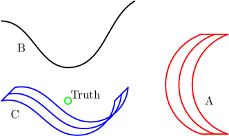
Figure 2: A: a model far from the truth (underlying distribution of observed data); B: close to the truth but sensitive to parameter; C (deep learning): close to the truth with many good local optima.

In fig. 2, model C displays the concepts of a DNN, where there are many good local optima. The performance is not sensitive to specific values of model parameters. On the lightlike neuromanifold $\mathcal{M}$, there are many directions that are very close to being lightlike. When a DNN model varies along these directions, the model slightly changes in terms of $\mathcal{I}(\bm{\theta})$, but their prediction on the samples measured by $\mathfrak{J}(\bm{\theta})$ are invariant. These directions count negatively towards the complexity, because these extra freedoms (dimensions of $\bm{\theta}$) occupy almost zero volume in the geometric sense, and are helpful to give a shorter code to future unseen samples.

To obtain a simpler expression, we consider the case that $\mathcal{I}(\bm{\theta})\equiv\mathcal{I}(\hat{\bm{\theta}})$ is both constant and diagonal in the interested region defined by eq. 22. In this case,

$$\log{V}\approx\frac{D}{2}\log 2\pi+D\log{}\varepsilon_{2}+\frac{1}{2}\log|\mathcal{I}(\hat{\bm{\theta}})+\varepsilon_{1}\bm{I}|.$$ (29)

On the other hand, as $D\to\infty$, the spectrum of the FIM $\mathcal{I}(\bm{\theta})$ will follow the density $\rho_{\mathcal{I}}(\bm{\theta})$. We plug these expressions into eq. 28, discard all lower-order terms, and get a simplified version of the razor

$$\mathcal{O}\approx -\log p(\bm{X}\,|\,\hat{\bm{\theta}})+\frac{D}{2}\log{N}+\frac{D}{2}\int_{0}^{\infty}\rho_{\mathcal{I}}(\lambda)\log\left(\lambda+\frac{1}{N\varepsilon_{2}^{2}}\right)\mathrm{d}\lambda,$$ (30)

where $\rho_{\mathcal{I}}$ denotes the spectral density of the Fisher information matrix.

H.1 Proof of Proposition 9

Assume $\mathfrak{J}(\hat{\bm{\theta}})$ has the spectral decomposition $\mathfrak{J}(\hat{\bm{\theta}})=\bm{Q}^{\intercal}\bm{\Lambda}\bm{Q}$, where $\bm{\Lambda}=\mathrm{diag}(\lambda_{1},\cdots,\lambda_{D})$ is a diagonal matrix.

By eq. 26,

$$R =\frac{1}{2}{\hat{\bm{\theta}}^{\intercal}}\bigg{[}N\mathfrak{J}(\hat{\bm{\theta}})-N\mathfrak{J}(\hat{\bm{\theta}})\bigg{(}N\mathfrak{J}(\hat{\bm{\theta}})+\frac{1}{\varepsilon_{2}^{2}}\bm{I}\bigg{)}^{-1}N\mathfrak{J}(\hat{\bm{\theta}})\bigg{]}\hat{\bm{\theta}}$$

$$=\frac{1}{2}{\hat{\bm{\theta}}^{\intercal}}\bm{Q}^{\intercal}\left[N\bm{\Lambda}-N^{2}\bm{\Lambda}^{2}\left(N\bm{\Lambda}+\frac{1}{\varepsilon_{2}^{2}}\bm{I}\right)^{-1}\right]\bm{Q}\hat{\bm{\theta}}.$$ (31)

Let $\bm{a}\vcentcolon=\bm{Q}\hat{\bm{\theta}}$, then

$$R =\frac{1}{2}\sum_{i=1}^{D}a_{i}^{2}\left(N\lambda_{i}-\frac{N^{2}\lambda_{i}^{2}}{N\lambda_{i}+\frac{1}{\varepsilon_{2}^{2}}}\right)$$

$$=\frac{1}{2}\sum_{i=1}^{D}a_{i}^{2}\frac{N\lambda_{i}}{N\lambda_{i}\varepsilon_{2}^{2}+1}$$

$$\leq\frac{1}{2}\sum_{i=1}^{D}a_{i}^{2}\frac{N\lambda_{m}}{N\lambda_{m}\varepsilon_{2}^{2}+1}$$

$$=\frac{1}{2}\|\bm{a}\|^{2}\frac{N\lambda_{m}}{N\lambda_{m}\varepsilon_{2}^{2}+1}$$

$$=\frac{1}{2}\|\hat{\bm{\theta}}\|^{2}\frac{N\lambda_{m}}{N\lambda_{m}\varepsilon_{2}^{2}+1}.$$ (32)

References

- [1] Hirotugu Akaike. A new look at the statistical model identification. IEEE Trans. Automat. Contr., 19(6):716–723, 1974.
- [2] Guillaume Alain, Nicolas Le Roux, and Pierre-Antoine Manzagol. Negative eigenvalues of the Hessian in deep neural networks. In ICLR’18 workshop, 2018. arXiv:1902.02366 [cs.LG].
- [3] Shun-ichi Amari. Information Geometry and Its Applications, volume 194 of Applied Mathematical Sciences. Springer, Japan, 2016.
- [4] Shun-ichi Amari, Tomoko Ozeki, Ryo Karakida, Yuki Yoshida, and Masato Okada. Dynamics of learning in MLP: Natural gradient and singularity revisited. Neural Computation, 30(1):1–33, 2018.
- [5] Toshiki Aoki and Katsuhiko Kuribayashi. On the category of stratifolds. Cahiers de Topologie et Géométrie Différentielle Catégoriques, LVIII(2):131–160, 2017. arXiv:1605.04142 [math.CT].
- [6] Oguzhan Bahadir and Mukut Mani Tripathi. Geometry of lightlike hypersurfaces of a statistical manifold, 2019. arXiv:1901.09251 [math.DG].
- [7] Vijay Balasubramanian. MDL, Bayesian inference and the geometry of the space of probability distributions. In Advances in Minimum Description Length: Theory and Applications, pages 81–98. MIT Press, Cambridge, Massachusetts, 2005.
- [8] A. Barron, J. Rissanen, and Bin Yu. The minimum description length principle in coding and modeling. IEEE Transactions on Information Theory, 44(6):2743–2760, 1998.
- [9] Léonard Blier and Yann Ollivier. The description length of deep learning models. In Advances in Neural Information Processing Systems 31, pages 2216–2226. Curran Associates, Inc., NY 12571, USA, 2018.
- [10] Ovidiu Calin. Deep learning architectures. Springer, London, 2020.
- [11] Ovidiu Calin and Constantin Udrişte. Geometric modeling in probability and statistics. Springer, Cham, 2014.
- [12] Yu Cheng, Duo Wang, Pan Zhou, and Tao Zhang. Model compression and acceleration for deep neural networks: The principles, progress, and challenges. IEEE Signal Processing Magazine, 35(1):126–136, 2018.
- [13] Laurent Dinh, Razvan Pascanu, Samy Bengio, and Yoshua Bengio. Sharp minima can generalize for deep nets. In International Conference on Machine Learning, volume 70 of Proceedings of Machine Learning Research, pages 1019–1028, 2017.
- [14] Krishan Duggal. A review on unique existence theorems in lightlike geometry. Geometry, 2014, 2014. Article ID 835394.
- [15] Krishan Duggal and Aurel Bejancu. Lightlike Submanifolds of Semi-Riemannian Manifolds and Applications, volume 364 of Mathematics and Its Applications. Springer, Netherlands, 1996.
- [16] Pascal Mattia Esser and Frank Nielsen. Towards modeling and resolving singular parameter spaces using stratifolds. arXiv preprint arXiv:2112.03734, 2021.
- [17] Xinlong Feng and Zhinan Zhang. The rank of a random matrix. Applied Mathematics and Computation, 185(1):689–694, 2007.
- [18] Adam Gaier and David Ha. Weight agnostic neural networks. In Advances in Neural Information Processing Systems 32, pages 5365–5379. Curran Associates, Inc., NY 12571, USA, 2019.
- [19] Xavier Glorot, Antoine Bordes, and Yoshua Bengio. Deep sparse rectifier neural networks. In International Conference on Artificial Intelligence and Statistics, volume 15 of Proceedings of Machine Learning Research, pages 315–323, 2011.
- [20] Ian Goodfellow, Yoshua Bengio, and Aaron Courville. Deep learning. MIT press, Cambridge, Massachusetts, 2016.
- [21] Peter Grünwald and Teemu Roos. Minimum description length revisited. International Journal of Mathematics for Industry, 11(01), 2020.
- [22] Peter D. Grünwald. The Minimum Description Length Principle. Adaptive Computation and Machine Learning series. The MIT Press, Cambridge, Massachusetts, 2007.
- [23] Tomohiro Hayase and Ryo Karakida. The spectrum of Fisher information of deep networks achieving dynamical isometry. In International Conference on Artificial Intelligence and Statistics, pages 334–342, 2021.
- [24] Masahito Hayashi. Large deviation theory for non-regular location shift family. Annals of the Institute of Statistical Mathematics, 63(4):689–716, 2011.
- [25] Sepp Hochreiter and Jürgen Schmidhuber. Flat minima. Neural Computation, 9(1):1–42, 1997.
- [26] Harold Hotelling. Spaces of statistical parameters. Bull. Amer. Math. Soc, 36:191, 1930.
- [27] Itay Hubara, Matthieu Courbariaux, Daniel Soudry, Ran El-Yaniv, and Yoshua Bengio. Binarized neural networks. In Advances in Neural Information Processing Systems 29, pages 4107–4115. Curran Associates, Inc., NY 12571, USA, 2016.
- [28] Varun Jain, Amrinder Pal Singh, and Rakesh Kumar. On the geometry of lightlike submanifolds of indefinite statistical manifolds, 2019. arXiv:1903.07387 [math.DG].
- [29] Ruichao Jiang, Javad Tavakoli, and Yiqiang Zhao. Weyl prior and Bayesian statistics. Entropy, 22(4), 2020.
- [30] Ryo Karakida, Shotaro Akaho, and Shun-ichi Amari. Universal statistics of Fisher information in deep neural networks: Mean field approach. In International Conference on Artificial Intelligence and Statistics, volume 89 of Proceedings of Machine Learning Research, pages 1032–1041, 2019.
- [31] Ryo Karakida, Shotaro Akaho, and Shun-ichi Amari. Pathological Spectra of the Fisher Information Metric and Its Variants in Deep Neural Networks. Neural Computation, 33(8):2274–2307, 2021.
- [32] David C Kay. Schaum’s outline of theory and problems of tensor calculus. McGraw-Hill, New York, 1988.
- [33] Andreĭ Nikolaevich Kolmogorov. Sur la notion de la moyenne. G. Bardi, tip. della R. Accad. dei Lincei, Rome, Italy, 1930.
- [34] Osamu Komori and Shinto Eguchi. A unified formulation of -Means, fuzzy -Means and Gaussian mixture model by the Kolmogorov–Nagumo average. Entropy, 23(5):518, 2021.
- [35] Frederik Kunstner, Philipp Hennig, and Lukas Balles. Limitations of the empirical Fisher approximation for natural gradient descent. In Advances in Neural Information Processing Systems 32, pages 4158–4169. Curran Associates, Inc., NY 12571, USA, 2019.
- [36] D.N. Kupeli. Singular Semi-Riemannian Geometry, volume 366 of Mathematics and Its Applications. Springer, Netherlands, 1996.
- [37] Stefan L Lauritzen. Statistical manifolds. Differential geometry in statistical inference, 10:163–216, 1987.
- [38] Chunyuan Li, Heerad Farkhoor, Rosanne Liu, and Jason Yosinski. Measuring the intrinsic dimension of objective landscapes. In International Conference on Learning Representations (ICLR), 2018.
- [39] Tengyuan Liang, Tomaso Poggio, Alexander Rakhlin, and James Stokes. Fisher-Rao metric, geometry, and complexity of neural networks. In International Conference on Artificial Intelligence and Statistics, volume 89 of Proceedings of Machine Learning Research, pages 888–896, 2019.
- [40] Wu Lin, Valentin Duruisseaux, Melvin Leok, Frank Nielsen, Mohammad Emtiyaz Khan, and Mark Schmidt. Simplifying momentum-based positive-definite submanifold optimization with applications to deep learning. In International Conference on Machine Learning, pages 21026–21050. PMLR, 2023.
- [41] David J.C. MacKay. Bayesian methods for adaptive models. PhD thesis, California Institute of Technology, 1992.
- [42] James A. Mingo and Roland Speicher. Free Probability and Random Matrices, volume 35 of Fields Institute Monographs. Springer, 2017.
- [43] In Jae Myung, Vijay Balasubramanian, and Mark A. Pitt. Counting probability distributions: Differential geometry and model selection. Proceedings of the National Academy of Sciences, 97(21):11170–11175, 2000.
- [44] Mitio Nagumo. Über eine Klasse der Mittelwerte. In Japanese journal of mathematics: transactions and abstracts, volume 7, pages 71–79. The Mathematical Society of Japan, 1930.
- [45] Naomichi Nakajima and Toru Ohmoto. The dually flat structure for singular models. Information Geometry, 4(1):31–64, 2021.
- [46] Behnam Neyshabur, Srinadh Bhojanapalli, David Mcallester, and Nati Srebro. Exploring generalization in deep learning. In Advances in Neural Information Processing Systems 30, pages 5947–5956. Curran Associates, Inc., NY 12571, USA, 2017.
- [47] Katsumi Nomizu, Nomizu Katsumi, and Takeshi Sasaki. Affine differential geometry: geometry of affine immersions. Cambridge Tracts in Mathematics. Cambridge university press, Cambridge, United Kingdom, 1994.
- [48] A Emin Orhan and Xaq Pitkow. Skip connections eliminate singularities. In International Conference on Learning Representations (ICLR), 2018.
- [49] Razvan Pascanu and Yoshua Bengio. Revisiting natural gradient for deep networks. In International Conference on Learning Representations (ICLR), 2014.
- [50] Jeffrey Pennington and Yasaman Bahri. Geometry of neural network loss surfaces via random matrix theory. In International Conference on Machine Learning, volume 70 of Proceedings of Machine Learning Research, pages 2798–2806, 2017.
- [51] Jeffrey Pennington, Samuel Schoenholz, and Surya Ganguli. The emergence of spectral universality in deep networks. In International Conference on Artificial Intelligence and Statistics, volume 84 of Proceedings of Machine Learning Research, pages 1924–1932, 2018.
- [52] Jeffrey Pennington and Pratik Worah. The spectrum of the Fisher information matrix of a single-hidden-layer neural network. In Advances in Neural Information Processing Systems 31, pages 5410–5419. Curran Associates, Inc., NY 12571, USA, 2018.
- [53] David Pollard. A note on insufficiency and the preservation of Fisher information. In From Probability to Statistics and Back: High-Dimensional Models and Processes–A Festschrift in Honor of Jon A. Wellner, pages 266–275. Institute of Mathematical Statistics, Beachwood, Ohio, 2013.
- [54] Maithra Raghu, Ben Poole, Jon Kleinberg, Surya Ganguli, and Jascha Sohl-Dickstein. On the expressive power of deep neural networks. In International Conference on Machine Learning, volume 70 of Proceedings of Machine Learning Research, pages 2847–2854, 2017.
- [55] Calyampudi Radhakrishna Rao. Information and the accuracy attainable in the estimation of statistical parameters. Bulletin of Cal. Math. Soc., 37(3):81–91, 1945.
- [56] Calyampudi Radhakrishna Rao. Information and the accuracy attainable in the estimation of statistical parameters. In Breakthroughs in statistics, pages 235–247. Springer, New York, NY, 1992.
- [57] Jorma Rissanen. Modeling by shortest data description. Automatica, 14(5):465–471, 1978.
- [58] Jorma Rissanen. Fisher information and stochastic complexity. IEEE Trans. Inf. Theory, 42(1):40–47, 1996.
- [59] Levent Sagun, Utku Evci, V. Ugur Guney, Yann Dauphin, and Leon Bottou. Empirical analysis of the Hessian of over-parametrized neural networks. In ICLR’18 workshop, 2018. arXiv:1706.04454 [cs.LG].
- [60] Salem Said, Hatem Hajri, Lionel Bombrun, and Baba C Vemuri. Gaussian distributions on Riemannian symmetric spaces: statistical learning with structured covariance matrices. IEEE Transactions on Information Theory, 64(2):752–772, 2017.
- [61] Gideon Schwarz. Estimating the dimension of a model. Ann. Stat., 6(2):461–464, 1978.
- [62] Alexander Soen and Ke Sun. On the variance of the Fisher information for deep learning. In Advances in Neural Information Processing Systems 34, pages 5708–5719, NY 12571, USA, 2021. Curran Associates, Inc.
- [63] Ke Sun and Frank Nielsen. Relative Fisher information and natural gradient for learning large modular models. In International Conference on Machine Learning, volume 70 of Proceedings of Machine Learning Research, pages 3289–3298, 2017.
- [64] Junnichi Takeuchi and S-I Amari. -parallel prior and its properties. IEEE Transactions on Information Theory, 51(3):1011–1023, 2005.
- [65] Philip Thomas. Genga: A generalization of natural gradient ascent with positive and negative convergence results. In International Conference on Machine Learning, volume 32 (2) of Proceedings of Machine Learning Research, pages 1575–1583, 2014.
- [66] Guillermo Valle-Pérez, Chico Q. Camargo, and Ard A. Louis. Deep learning generalizes because the parameter-function map is biased towards simple functions. In International Conference on Learning Representations (ICLR), 2019.
- [67] Christopher Stewart Wallace and D. M. Boulton. An information measure for classification. Computer Journal, 11(2):185–194, 1968.
- [68] Sumio Watanabe. Algebraic Geometry and Statistical Learning Theory, volume 25 of Cambridge Monographs on Applied and Computational Mathematics. Cambridge University Press, Cambridge, United Kingdom, 2009.
- [69] Haikun Wei, Jun Zhang, Florent Cousseau, Tomoko Ozeki, and Shun-ichi Amari. Dynamics of learning near singularities in layered networks. Neural computation, 20(3):813–843, 2008.
- [70] Yuki Yoshida, Ryo Karakida, Masato Okada, and Shun-ichi Amari. Statistical mechanical analysis of learning dynamics of two-layer perceptron with multiple output units. Journal of Physics A: Mathematical and Theoretical, 2019.
- [71] Chiyuan Zhang, Samy Bengio, Moritz Hardt, Benjamin Recht, and Oriol Vinyals. Understanding deep learning requires rethinking generalization. In International Conference on Learning Representations (ICLR), 2017.