Levenshtein Transformer

Abstract

Modern neural sequence generation models are built to either generate tokens step-by-step from scratch or (iteratively) modify a sequence of tokens bounded by a fixed length. In this work, we develop Levenshtein Transformer, a new partially autoregressive model devised for more flexible and amenable sequence generation. Unlike previous approaches, the basic operations of our model are insertion and deletion. The combination of them facilitates not only generation but also sequence refinement allowing dynamic length changes. We also propose a set of new training techniques dedicated at them, effectively exploiting one as the other’s learning signal thanks to their complementary nature. Experiments applying the proposed model achieve comparable or even better performance with much-improved efficiency on both generation (e.g. machine translation, text summarization) and refinement tasks (e.g. automatic post-editing). We further confirm the flexibility of our model by showing a Levenshtein Transformer trained by machine translation can straightforwardly be used for automatic post-editing.

1 Introduction

Neural sequence generation models are widely developed and deployed in tasks such as machine translation (Bahdanau et al., 2015; Vaswani et al., 2017). As we examine the current frameworks, the most popular autoregressive models generate tokens step-by-step. If not better, recent non-autoregressive approaches (Gu et al., 2018; Kaiser et al., 2018; Lee et al., 2018) have proved it possible to perform generation within a much smaller number of decoding iterations.

In this paper, we propose Levenshtein Transformer (LevT), aiming to address the lack of flexibility of the current decoding models. Notably, in the existing frameworks, the length of generated sequences is either fixed or monotonically increased as the decoding proceeds. This remains incompatible with human-level intelligence where humans can revise, replace, revoke or delete any part of their generated text. Hence, LevT is proposed to bridge this gap by breaking the in-so-far standardized decoding mechanism and replacing it with two basic operations — insertion and deletion.

We train the LevT using imitation learning. The resulted model contains two policies and they are executed in an alternate manner. Empirically, we show that LevT achieves comparable or better results than a standard Transformer model on machine translation and summarization, while maintaining the efficiency advantages benefited from parallel decoding similarly to  (Lee et al., 2018). With this model, we argue that the decoding becomes more flexible. For example, when the decoder is given an empty token, it falls back to a normal sequence generation model. On the other hand, the decoder acts as a refinement model when the initial state is a low-quality generated sequence. Indeed, we show that a LevT trained from machine translation is directly applicable to translation post-editing without any change. This would not be possible with any framework in the literature because generation and refinement are treated as two different tasks due to the model’s inductive bias.

One crucial component in LevT framework is the learning algorithm. We leverage the characteristics of insertion and deletion — they are complementary but also adversarial. The algorithm we propose is called “dual policy learning”. The idea is that when training one policy (insertion or deletion), we use the output from its adversary at the previous iteration as input. An expert policy, on the other hand, is drawn to provide a correction signal. Despite that, in theory, this learning algorithm is applicable to other imitation learning scenarios where a dual adversarial policy exists, in this work we primarily focus on a proof-of-concept of this algorithm landing at training the proposed LevT model.

To this end, we summarize the contributions as follows:

• We propose Levenshtein Transformer (LevT), a new sequence generation model composed of the insertion and deletion operations. This model achieves comparable or even better results than a strong Transformer baseline in both machine translation and text summarization, but with much better efficiency (up to $\times 5$ speed-up in terms of actual machine execution time);

• We propose a corresponding learning algorithm under the theoretical framework of imitation learning, tackling the complementary and adversarial nature of the dual policies;

• We recognize our model as a pioneer attempt to unify sequence generation and refinement, thanks to its built-in flexibility. With this unification, we empirically validate the feasibility of applying a LevT model trained by machine translation directly to translation post-editing, without any change.

2 Problem Formulation

2.1 Sequence Generation and Refinement

We unify the general problems of sequence generation and refinement by casting them to a Markov Decision Process (MDP) defined by a tuple $\left(\mathcal{Y},\mathcal{A},\mathcal{E},\mathcal{R},\bm{y_{0}}\right)$. We consider the setup consisting an agent interacting with an environment $\mathcal{E}$ which receives the agent’s editing actions and returns the modified sequence. We define $\mathcal{Y}=\mathcal{V}^{N_{\max}}$ as a set of discrete sequences up to length $N_{\max}$ where $\mathcal{V}$ is a vocabulary of symbols. At every decoding iteration, the agent receives an input $\bm{y}$ drawn from scratch or uncompleted generation, chooses an action $\bm{a}$ and gets a reward $r$. We use $\mathcal{A}$ to denote the set of actions and $\mathcal{R}$ for the reward function. Generally the reward function $\mathcal{R}$ measures the distance between the generation and the ground-truth sequence, $\mathcal{R}(\bm{y})=-\mathcal{D}(\bm{y},\bm{y}^{*})$ which can be any distance measurement such as the Levenshtein distance (Levenshtein, 1965). It is crucial to incorporate $\bm{y_{0}}\in\mathcal{Y}$ into the our formulation. As the initial sequence, the agent receives—when $\bm{y_{0}}$ is an already generated sequence from another system, the agent essentially learns to do refinement while it falls back to generation if $\bm{y_{0}}$ is an empty sequence. The agent is modeled by a policy, $\pi$, that maps the current generation over a probability distribution over $\mathcal{A}$. That is, $\pi:\mathcal{Y}\to P(\mathcal{A})$.

2.2 Actions: Deletion & Insertion

Following the above MDP formulation, with a subsequence $\bm{y}^{k}=(y_{1},y_{2},...,y_{n})$, the two basic actions – deletion and insertion – are called to generate $\bm{y}^{k+1}=\mathcal{E}(\bm{y}^{k},\bm{a}^{k+1})$. Here we let $y_{1}$ and $y_{n}$ be special symbols <s> and </s>, respectively. Since we mainly focus on the policy of a single round generation, the superscripts are omitted in this section for simplicity. For conditional generation like MT, our policy also includes an input of source information $\bm{x}$ which is also omitted here.

Deletion

The deletion policy reads the input sequence $\bm{y}$, and for every token $y_{i}\in\bm{y}$, the deletion policy $\pi^{\textrm{del}}(d|i,\bm{y})$ makes a binary decision which is 1 (delete this token) or 0 (keep it). We additionally constrain $\pi^{\textrm{del}}(0|1,\bm{y})=\pi^{\textrm{del}}(0|n,\bm{y})=1$ to avoid sequence boundary being broken. The deletion classifier can also be seen as a fine-grained discriminator used in GAN (Goodfellow et al., 2014) where we predict “fake” or “real” labels for every predicted token.

Insertion

In this work, it is slightly more complex to build the insertion atomic because it involves two phases: placeholder prediction and token prediction so that it is able to insert multiple tokens at the same slot. First, among all the possible inserted slots ($y_{i},y_{i+1}$) in $\bm{y}$, $\pi^{\textrm{plh}}(p|i,\bm{y})$ predicts the possibility of adding one or several placeholders. In what follows, for every placeholder predicted as above, a token prediction policy $\pi^{\textrm{tok}}(t|i,\bm{y})$ replaces the placeholders with actual tokens in the vocabulary. The two-stage insertion process can also be viewed as a hybrid of Insertion Transformer (Stern et al., 2019) and masked language model (MLM, Devlin et al., 2018; Ghazvininejad et al., 2019).

Policy combination

Recall that our two operations are complementary. Hence we combine them in an alternate fashion. For example in sequence generation from the empty, insertion policy is first called and it is followed by deletion, and then repeat till the certain stopping condition is fulfilled. Indeed, it is possible to leverage the parallelism in this combination. We essentially decompose one iteration of our sequence generator into three phases: “delete tokens – insert placeholders – replace placeholders with new tokens”. Within each stage, all operations are performed in parallel. More precisely, given the current sequence $\bm{y}=(y_{0},\ldots,y_{n})$, and suppose the action to predict is $\bm{a}=\{\underbrace{d_{0},\ldots d_{n}}_{\bm{d}};\underbrace{p_{0},\ldots,p_{n-1}}_{\bm{p}};\underbrace{t_{0}^{1},\ldots t_{0}^{p_{0}},\ldots,t_{n-1}^{p_{n-1}}}_{\bm{t}}\}$, the policy for one iteration is:

$$\pi(\bm{a}|\bm{y})=\prod_{d_{i}\in\bm{d}}\pi^{\textrm{del}}(d_{i}|i,\bm{y})\cdot\prod_{p_{i}\in\bm{p}}\pi^{\textrm{plh}}(p_{i}|i,\bm{y}^{\prime})\cdot\prod_{t_{i}\in\bm{t}}\pi^{\textrm{tok}}(t_{i}|i,\bm{y}^{\prime\prime}),$$ (1)

where $\bm{y}^{\prime}=\mathcal{E}(\bm{y},\bm{d})$ and $\bm{y}^{\prime\prime}=\mathcal{E}(\bm{y}^{\prime},\bm{p})$. We parallelize the computation within each sub-tasks.

3 Levenshtein Transformer

In this section, we cover the specs of Levenshtein Transformer and the dual-policy learning algorithm. Overall our model takes a sequence of tokens (or none) as the input then iteratively modify it by alternating between insertion and deletion, until the two policies combined converge. We describe the detailed learning and inference algorithms in the Appendix.

Figure 1: The illustration of the proposed Levenshtein Transformer decoder for one refinement iteration. The same architecture can be applied for three different tasks with specific classifiers. For simplicity, the encoder-decoder attention is omitted within each Transformer-Block.

3.1 Model

We use Transformer (Vaswani et al., 2017) as the basic building block. For conditional generation, the source $\bm{x}$ is included in each TransformerBlock. The states from the $l$-th block are:

$$\bm{h}_{0}^{(l+1)},\bm{h}_{1}^{(l+1)},...,\bm{h}_{n}^{(l+1)}=\left\{\begin{matrix}E_{y_{0}}+P_{0},E_{y_{1}}+P_{1},...,E_{y_{n}}+P_{n},&l=0\\ \text{TransformerBlock}_{l}(\bm{h}_{0}^{(l)},\bm{h}_{1}^{(l)},...,\bm{h}_{n}^{(l)}),&l>0\end{matrix}\right.$$ (2)

where $E\in\mathbb{R}^{|\mathcal{V}|\times d_{\text{model}}}$ and $P\in\mathbb{R}^{N_{\text{max}}\times d_{\text{model}}}$ are the token and position embeddings, respectively. We show the illustration of the proposed LevT model for one refinement (delete, insert) as Figure 1.

Policy Classifiers

The decoder outputs ($\bm{h}_{0},\bm{h}_{2},...,\bm{h}_{n}$) are passed to three policy classifiers:

1. Deletion Classifier: LevT scans over the input tokens (except for the boundaries) and predict “deleted” ($0$) or “kept” ($1$) for each token position,

   $$\pi_{\theta}^{\mathrm{del}}(d|i,\bm{y})=\operatorname*{\text{softmax}}\left(\bm{h}_{i}\cdot A^{\top}\right),\ \ i=1,\ldots n-1,$$ (3)

   where $A\in\mathbb{R}^{2\times d_{\text{model}}}$, and we always keep the boundary tokens.

2. Placeholder Classifier: LevT predicts the number of tokens to be inserted at every consecutive position pairs, by casting the representation to a categorical distribution:

   $$\pi_{\theta}^{\mathrm{plh}}(p|i,\bm{y})=\operatorname*{\text{softmax}}\left(\texttt{concat}(\bm{h}_{i},\bm{h}_{i+1})\cdot B^{\top}\right),\ \ i=0,\ldots n-1,$$ (4)

   where $B\in\mathbb{R}^{(K_{\max}+1)\times(2d_{\text{model}})}$. Based on the number ($0\sim K_{\max}$) of tokens it predicts, we insert the considered number of placeholders at the current position. In our implementation, placehoder is represented by a special token <PLH> which was reserved in the vocabulary.

3. Token Classifier: following the placeholder prediction, LevT needs to fill in tokens replacing all the placeholders. This is achieved by training a token predictor as follow:

   $$\pi_{\theta}^{\mathrm{tok}}(t|i,\bm{y})=\operatorname*{\text{softmax}}\left(\bm{h}_{i}\cdot C^{\top}\right),\ \ \forall y_{i}=\texttt{<PLH>},$$ (5)

   where $C\in\mathbb{R}^{|\mathcal{V}|\times d_{\text{model}}}$ with parameters being shared with the embedding matrix.

Weight Sharing

Our default implementation always assumes the three operations to share the same Transformer backbone to benefit features learned from other operations. However, it is also possible to disable weight sharing and train separate decoders for each operations, which increases the capacity of the model while does not affect the overall inference time.

Early Exit

Although it is parameter-efficient to share the same Transformer architecture across the above three heads, there is room for improvement as one decoding iteration requires three full passes of the network. To make trade-off between performance and computational cost, we propose to perform early exit (attaching the classifier to an intermediate block instead of the last one) for $\pi^{\textrm{del}}$ and $\pi^{\textrm{plh}}$ to reduce computation while keeping $\pi^{\textrm{tok}}$ always based on the last block, considering that token prediction is usually more challenging than the other two tasks.

3.2 Dual-policy Learning

Imitation Learning

We use imitation learning to train the Levenshtein Transformer. Essentially we let the agent imitate the behaviors that we draw from some expert policy $\pi^{*}$. The expert policy is derived from direct usage of ground-truth targets or less noisy version filtered by sequence distillation (Kim and Rush, 2016). The objective is to maximize the following expectation:

$$\begin{split}\underbrace{\mathbb{E}_{\begin{subarray}{l}\bm{y}_{\textrm{del}}\sim d_{\tilde{\pi}_{\textrm{del}}}\\ \bm{d}^{*}\sim\pi^{*}\end{subarray}}\!\!\!\sum_{d^{*}_{i}\in\bm{d}^{*}}\!\log\pi_{\theta}^{\mathrm{del}}(d^{*}_{i}|i,\bm{y}_{\textrm{del}})}_{\textit{Deletion Objective}}+\underbrace{\mathbb{E}_{\begin{subarray}{l}\bm{y}_{\textrm{ins}}\sim d_{\tilde{\pi}_{\textrm{ins}}}\\ \bm{p}^{*},\bm{t}^{*}\sim\pi^{*}\end{subarray}}\!\!\left[\sum_{p^{*}_{i}\in\bm{p}^{*}}\!\log\pi_{\theta}^{\mathrm{plh}}(p^{*}_{i}|i,\bm{y}_{\textrm{ins}})+\!\!\!\sum_{t^{*}_{i}\in\bm{t}^{*}}\!\log\pi_{\theta}^{\mathrm{tok}}(t^{*}_{i}|i,\bm{y}^{\prime}_{\textrm{ins}})\right]}_{\textit{Insertion Objective}},\end{split}$$

where $\bm{y}^{\prime}_{\textrm{ins}}$ is the output after inserting palceholders $\bm{p}^{*}$ upon $\bm{y}_{\textrm{ins}}$. $\tilde{\pi}_{\textrm{del}}$, $\tilde{\pi}_{\textrm{ins}}$ are the roll-in polices and we repeatedly draw states (sequences) from their induced state distribution $d_{\tilde{\pi}_{\textrm{del}}},d_{\tilde{\pi}_{\textrm{ins}}}$. These states are first executed by the expert policy returning the suggested actions by the expert, and then we maximize the conditional log-likelihood over them.

Figure 2: The data-flow of learning.

By definition, the roll-in policy determines the state distribution fed to $\pi_{\theta}$ during training. In this work, we have two strategies to construct the roll-in policy — adding noise to the ground-truth or using the output from the adversary policy. Figure 2 shows a diagram of this learning paradigm. We formally write down the roll-in policies as follows.

1. Learning to Delete: we design the $\tilde{\pi}_{\textrm{del}}$ as a stochastic mixture between the initial input $\bm{y}^{0}$ or the output by applying insertion from the model with some mixture factor $\alpha\in[0,1]$:

   $$d_{\tilde{\pi}_{\textrm{del}}}=\{\bm{y}^{0}\ \ \ \text{if}\ \ u<\alpha\ \ \text{else}\ \ \ \mathcal{E}\left(\mathcal{E}\left(\bm{y}^{\prime},\bm{p}^{*}\right),\tilde{\bm{t}}\right),\ \ \bm{p}^{*}\sim\pi^{*},\tilde{\bm{t}}\sim\pi_{\theta}\}$$ (6)

   where $u\sim\text{Uniform}[0,1]$ and $\bm{y}^{\prime}$ is any sequence ready to insert tokens. $\tilde{\bm{t}}$ is obtained by sampling instead of doing argmax from Eq. (5).

2. Learning to Insert: similar to the deletion step, we apply a mixture of the deletion output and a random word dropping sequence of the round-truth, inspired by recent advances of training masked language model (Devlin et al., 2018). We use random dropping as a form of noise injection to encourage more exploration. Let $\beta\in[0,1]$ and $u\sim\text{Uniform}[0,1]$,

   $$d_{\tilde{\pi}_{\textrm{ins}}}=\{\mathcal{E}\left(\bm{y}^{0},\bm{d}^{*}\right),\ \ \bm{d}^{*}\sim\pi^{*}\ \ \ \text{if}\ \ u<\beta\ \ \text{else}\ \ \ \mathcal{E}\left(\bm{y}^{*},\tilde{\bm{d}}\right),\ \ \tilde{\bm{d}}\sim\pi^{\textsc{rnd}}\}$$ (7)

Expert Policy

It is crucial to construct an expert policy in imitation learning which cannot be too hard or too weak to learn from. Specifically, we considered two types of experts:

1. Oracle: One way is to build an oracle which accesses to the ground-truth sequence. It returns the optimal actions $\bm{a}^{*}$ (either oracle insertion $\bm{p}^{*},\bm{t}^{*}$ or oracle deletion $\bm{d}^{*}$) by:

   $$\bm{a}^{*}=\operatorname*{arg\!\ min}_{\bm{a}}\mathcal{D}(\bm{y}^{*},\mathcal{E}(\bm{y},\bm{a}))$$ (8)

   Here, we use the Levenshtein distance (Levenshtein, 1965) as $\mathcal{D}$ considering it is possible to obtain the action suggestions efficiently by dynamic programming.

2. Distillation: We also explore to use another teacher model to provide expert policy, which is known as sequence-level knowledge distillation (Kim and Rush, 2016). This technique has been widely used in previous approaches for nonauoregressive generation (Gu et al., 2018). More precisely, we first train an autoregressive teacher model using the same datasets and then replace the ground-truth sequence $\bm{y^{*}}$ by the beam-search result of this teacher-model, $\bm{y^{\textsc{ar}}}$. We use the same mechanism to find the suggested option as using the ground-truth oracle.

3.3 Inference

Greedy Decoding

At inference time, we apply the trained model over the initial sequence $\bm{y}^{0}$ for several iterations. We greedily pick up the actions associated with high probabilities in Eq. (3)(4)(5). Moreover, we find that using search (instead of greedy decoding) or nosiy parallel decoding (Cho, 2016) does not yield much gain in LevT. This observation is quite opposite to what has been widely discovered in autoregressive decoding. We hypothesize there may be two reasons leading to this issue: (i) The local optimal point brought by greedy decoding in autoregressive models is often far from the optimal point globally. Search techniques resolve this issue with tabularization. In our case, however, because LevT inserts or deletes tokens dynamically, it could easily revoke the tokens that are found sub-optimal and re-insert better ones; (ii) the log-probability of LevT is not a good metric to select the best output. However, we do believe to see more improvements if we include an external re-ranker, e.g. an autoregressive teacher model. We leave this discussion in the future work.

Termination Condition

The decoding stops when one of the following two conditions is fulfilled:

1. Looping: Generation is terminated if two consecutive refinement iterations return the same output which can be (i) there are no words to delete or insert; (ii) the agent gets stuck in an infinite loop: i.e. the insertion and deletion counter each other and keep looping.

2. Timeout: We further set a maximum number of iterations (timeout) to guarantee a constant-time complexity in the worst case (Lee et al., 2018; Ghazvininejad et al., 2019).

Penalty for Empty Placeholders

Similar to  Stern et al. (2019), we add a penalty to insert “empty” placeholder in decoding. Overly inserting “empty” placeholders may result in shorter output. A penalty term $\gamma\in[0,3]$ is subtracted from the logits of $0$ in Eq. (4).

4 Experiments

We validate the efficiency, effectiveness, and flexibility of Levenshtein Transformer extensively across three different tasks — machine translation (MT), text summarization (TS) and automatic post-editing (APE) for machine translation, from both generation (§4.1) and refinement (§4.2) perspectives.

Table 1: Generation quality (BLEU $\uparrow$, ROUGE-1/2/L $\uparrow$) and latency (ms $\downarrow$) as well as the average number of decoder iterations ($I_{\textsc{dec}}$) on the standard test sets for LevT and the autoregressive baseline (with both greedy and beam-search outputs). We show the results of LevT trained from both oracle and the autoregressive teacher model.

	Dataset	Metric	Transformer		Levenshtein Transformer
			greedy	beam4	oracle	distillation
Quality $\uparrow$	Ro-En	BLEU	31.67	32.30	33.02	33.26
	En-De	BLEU	26.89	27.17	25.20	27.27
	En-Ja	BLEU	42.86	43.68	42.36	43.17
	Gigaword	ROUGE-1	37.31	37.87	36.14	37.40
		ROUGE-2	18.10	18.92	17.14	18.33
		ROUGE-L	34.65	35.13	34.34	34.51
Speed $\downarrow$	Ro-En	Latency (ms) /$I_{\textsc{dec}}$	326 / 27.1	349 / 27.1	97 / 2.19	90 / 2.03
	En-De	Latency (ms) /$I_{\textsc{dec}}$	343 / 28.1	369 / 28.1	126 / 2.88	92 / 2.05
	En-Ja	Latency (ms) /$I_{\textsc{dec}}$	261 / 22.6	306 / 22.6	112 / 2.61	106 / 1.97
	Gigaword	Latency (ms) /$I_{\textsc{dec}}$	116 / 10.1	149 / 10.1	98 / 2.32	84 / 1.73

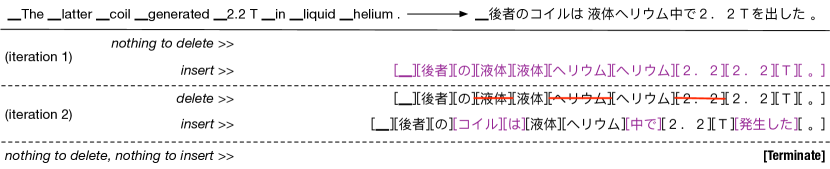
Figure 3: An example of WAT’17 En-Ja translation with two decoder iterations by LevT. We present the inserted tokens in purple and deleted tokens with red strikethrough

.

4.1 Sequence Generation

For the sequence generation perspective, we evaluate LevT model on MT and TS. As a special case, sequence generation assumes empty $\bm{y}^{0}=\textsc{<s></s>}$ as input and no initial deletion is applied.

Data & Evaluation

We use three diversified language pairs for MT experiments: WMT’16 Romanian-English (Ro-En), WMT’14 English-German (En-De) and WAT2017 Small-NMT English-Japanese (En-Ja, Nakazawa et al., 2017). The TS experiments use preprocessed data from the Annotated English Gigaword (Gigaword, Rush et al., 2015). We learn byte-pair encoding (BPE, Sennrich et al., 2016) vocabulary on tokenized data. Detailed dataset statistics can be found in the Appendix. For evaluation metrics, we use BLEU (Papineni et al., 2002) for MT and ROUGE-1,2,L (Lin, 2004) for TS. Before computing the BLEU scores for Japanese output, we always segment Japanese words using KyTea .

Models & Training

We adopt the model architecture of Transformer base (Vaswani et al., 2017) for the proposed LevT model and the autoregressive baseline. All the Transformer-based models are trained on $8$ Nvidia Volta GPUs with maximum $300K$ steps and a total batch-size of around $65,536$ tokens per step (We leave more details to the Appendix).

Overall results

We present our main results on the generation quality and decoding speed in Table 1. We measure the speed by the averaged generation latency of generating one sequence at a time on single Nvidia V100 GPU. To remove the implementation bias, we also present the number of decoder iterations as a reference. It can be concluded that for both MT and summarization tasks, our proposed LevT achieves comparable and sometimes better generation quality compared to the strong autoregressive baseline, while LevT is much more efficient at decoding. A translation example is shown in Figure 3 and we leave more in Appendix. We conjecture that this is due to that the output of the teacher model possesses fewer modes and much less noisy than the real data. Consequently, LevT needs less number of iterations to converge to this expert policy.

Table 2: Ablation study for Levenshtein Transformer on En-De (a) and Ro-En (b) translation tasks.

(a) Test BLEU for variant weight sharing. Baseline scores from Lee et al. (IT, 2018), Ghazvininejad et al. (MaskT, 2019) are included for reference.

sharing	none	$\textrm{plh},\textrm{ins}$	$\textrm{ins},\textrm{del}$	all	IT	MaskT
oracle	$-$	25.50	$-$	25.20	$-$	$-$
distill	25.11	27.73	24.90	27.27	21.61	26.56

(b) Test BLEU and deletion loss with variant roll-in polices.

roll-in	BLEU	NLL(del)
Ours	33.02	$\approx$ 0.202
DAE	31.78	$\approx$ 0.037

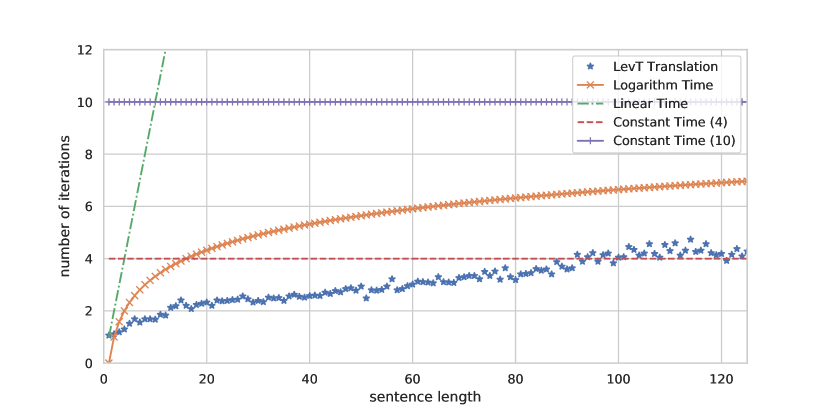
(a) Average number of refinement iterations v.s. length measured on monolingual corpus. For most of the time, LevT decodes with much smaller number (generally, 1$\sim$4) of iterations.

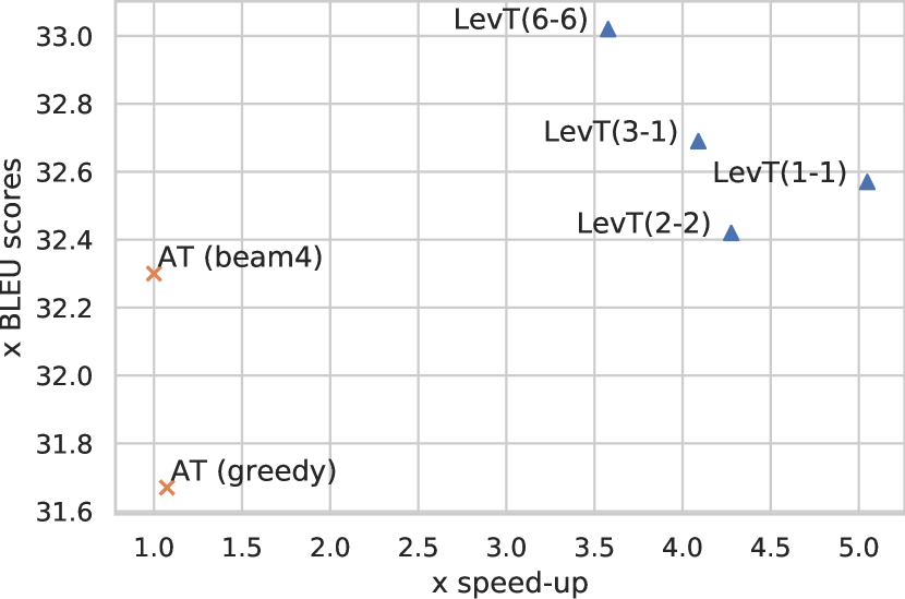
(b) BLEU v.s. speed-up for LevT across variant early-exits and the autoregressive baselines on the test set of Ro-En.

Figure 4: Plots showing the decoding efficiency of the proposed Levenshtein Transformer.

Ablation on Efficiency

As shown in Figure 4(a), we plot the average number of iterations over the length of input over a monolingual corpus. LevT learns to properly adjust the decoding time accordingly. We also explore the variants of “early exit” where we denote LevT($m$-$n$) as a model with $m$ and $n$ blocks for deletion (Eq. (3)) and placeholder prediction (Eq. (4)) respectively. Figure 4(b) shows that although it compromises the quality a bit, our model with early exit achieves up to $\times 5$ speed-up (execution time) comparing against a strong autoregressive Transformer using beam-search.

Ablation on Weight Sharing

We also evaluate LevT with different weight sharing as noted in §3.1. The results of models trained with oracle or distillation are listed in Table 2(a). We observe that weight-sharing is beneficial especially between the two insertion operations (placeholder and token classifiers). Also, it shows another $+0.5$ BLEU improvement by not sharing the deletion operation with insertion compared to the default setting, which may indicate that insertion and deletion capture complementary information, requiring larger capacity by learning them separately.

Importance of mixture roll-in policy

We perform an ablation study on the learning algorithm. Specifically, we train a model with no mixing of the $\pi_{\theta}$ in Equation (6). We name this experiment by DAE due to its resemblance to a denoising autoencoder. We follow closely a standard pipeline established by Lee et al. (2018). Table 2(b) shows this comparison. As we can see that the deletion loss from DAE is much smaller while the generation BLEU score is inferior. We conjecture that this is caused by the mismatch between the states from the model and the roll-in policy in training the DAE.

v.s. Exiting Refinement-based Models

Table 2(a) also includes results from two relevant recent works which also incorporate iterative refinement in non-autoregressive sequence generation. For fair comparison, we use the result with length beam $1$ from Ghazvininejad et al. (2019). Although both approaches use similar “denosing” objectives to train the refinement process, our model explicitly learns “insertion” and “deletion” in a dual-policy learning fashion, and outperforms both models.

4.2 Sequence Refinement

We evaluate LevT’s capability of refining sequence outputs on the APE task. In this setting, inputs are pairs of the source sequence and a black-box MT system generation. The ground-truth outputs are from real human edits with expansion using synthetic data.

Dataset

We follow a normal protocol in the synthetic APE experiments (Grangier and Auli, 2017): we first train the input MT system on half of the dataset. Then we will train a refinement model on the other half based on the output produced by the MT model trained in the previous phase. For the real APE tasks, we use the data from WMT17 Automatic Post-Editing Shared Task on En-De. It contains both real PE triples and a large-scale synthetic corpus.

Table 3: Performance (BLEU $\uparrow$ / case-sensitive TER $\downarrow$) comparison on APE. “do nothing” represents the results of the original MT system output; the autoregressive model uses beam-size $4$. For the proposed LevT, we use “scratch” to denote training from scratch on the APE triple data, and use “zero-shot” to denote applying an MT pre-trained LevT model directly for post-editing tasks. The same model can be further fine-tuned. All scores with underlines are from the model trained with an autoregressive teacher model (distillation) as the expert policy.

Dataset		MT	Do-Nothing	Transformer	Levenshtein Transformer
		system			Scratch	Zero-shot	Fine-tune
Synthetic	Ro-En	PBMT	27.5 / 52.6	28.9 / 52.8	29.1 / 50.4	30.1 / 51.7	$-$
		NMT	26.2 / 56.5	26.9 / 55.6	28.3 / 53.6	28.0 / 55.8	$-$
	En-De	PBMT	15.4 / 69.4	22.8 / 61.0	25.8 / 56.6	16.5 / 69.6	$-$
	En-Ja	NMT	37.7 / 48.0	41.0 / 44.9	42.2 / 44.3	39.4 / 47.5	$-$
Real	En-De	PBMT	62.5 / 24.5	67.2 / 22.1	66.9 / 21.9	59.6 / 28.7	70.1 / 19.2

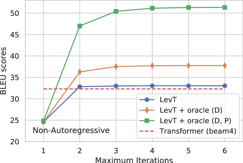
(a) Test set BLEU scores for WMT Ro-En

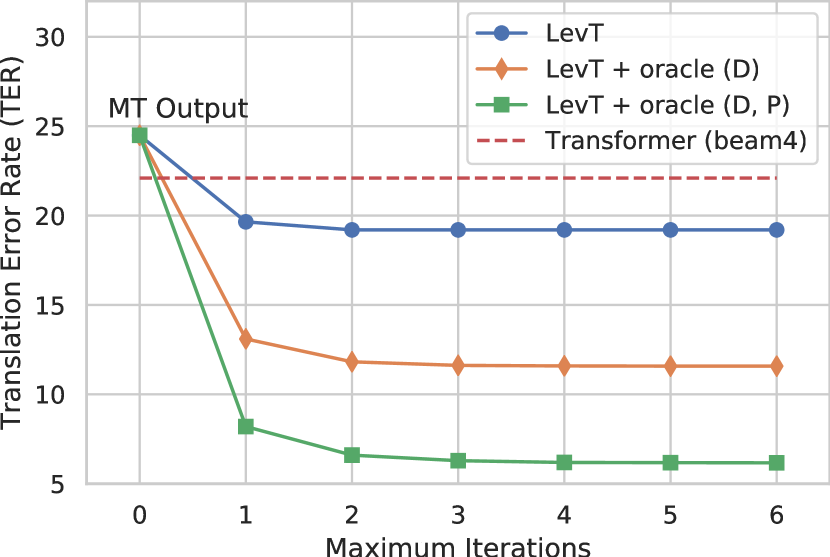
(b) Test set TER scores for Real APE En-De

Figure 5: MT & PE Performance v.s. Timeout iterations w/o oracle instructions.

Models & Evaluation

The baseline model is a standard Transformer encoding the concatenation of the source and the MT system’s output. For the MT system here, we want some imperfect systems that need to be refined. We consider a statistical phrase-based MT system (PBMT, Koehn et al., 2003) and an RNN-based NMT system (Bahdanau et al., 2015). Apart from BLEU scores, we additionally apply translation error rate (TER, Snover et al., 2006) as it is widely used in the APE literature.

Overall results

We show the major comparison in Table 3. When training from scratch, LevT consistently improves the performance of the input MT system (either PBMT or NMT). It also achieves better performance than the autoregressive Transformer in most of the cases.

Pre-training on MT

Thanks to the generality of the LevT model, we show it is feasible to directly apply the LevT model trained by generation onto refinement tasks — in this case — MT and APE. We name this a “zero-shot post-editing” setting. According to Table 3, the pre-trained MT models are always capable of improving the initial MT input in the synthetic tasks.

The real APE task, however, differs quite a bit from the synthetic tasks because human translators normally only fix a few spotted errors. This ends up with very high BLEU scores even for the “Do-nothing” column. However, the pre-trained MT model achieves the best results by fine-tuning on the PE data indicating that LevT is able to leverage the knowledge for generation and refinement.

Collaborate with Oracle

Thanks to the saperation of insertion and deletion operations, LevT has better interpretability and controllability. For example, we test the ability that LevT adapts oracle (e.g. human translators) instructions. As shown in Figure 5, both MT and PE tasks have huge improvement if every step the oracle deletion is given. This goes even further if the oracle provides both the correct deletion and the number of placehoders to insert. It also sheds some light upon computer-assisted text editing for human translators.

5 Related Work

Non-Autoregressive and Non-Monotonic Decoding

Breaking the autoregressive constraints and monotonic (left-to-right) decoding order in classic neural sequence generation systems has recently attracted much interest. Stern et al. (2018); Wang et al. (2018) designed partially parallel decoding schemes to output multiple tokens at each step. Gu et al. (2018) proposed a non-autoregressive framework using discrete latent variables, which was later adopted in Lee et al. (2018) as iterative refinement process. Ghazvininejad et al. (2019) introduced the masked language modeling objective from BERT (Devlin et al., 2018) to non-autoregressively predict and refine translations. Welleck et al. (2019); Stern et al. (2019); Gu et al. (2019) generate translations non-monotonically by adding words to the left or right of previous ones or by inserting words in arbitrary order to form a sequence.

Editing-Based Models

Several prior works have explored incorporating “editing” operations for sequence generation tasks. For instance, Novak et al. (2016) predict and apply token substitutions iteratively on phase-based MT system outputs using convolutional neural network. QuickEdit (Grangier and Auli, 2017) and deliberation network (Xia et al., 2017) both consist of two autoregressive decoders where the second decoder refines the translation generated by the first decoder. Guu et al. (2018) propose a neural editor which learned language modeling by first retrieving a prototype and then editing over that. Freitag et al. (2019) correct patterned errors in MT system outputs using transformer models trained on monolingual data. Additionally, the use of Levenshtein distance with dynamic programming as the oracle policy were also proposed in  Sabour et al. (2018); Dong et al. (2019). Different from these work, the proposed model learns a non-autoregressive model which simultaneously inserts and deletes multiple tokens iteratively.

6 Conclusion

We propose Levenshtein Transformer, a neural sequence generation model based on insertion and deletion. The resulted model achieves performance and decoding efficiency, and embraces sequence generation to refinement in one model. The insertion and deletion operations are arguably more similar to how human writes or edits text. For future work, it is potential to extend this model to human-in-the-loop generation.

Appendix A Learning & Inference Algorithm

We present the detailed algorithms for learning and decoding from Levenshtein Transformer as follows. For simplicity, we always omit the source information $\bm{x}$ in conditional sequence generation tasks such as machine translation which is handled by the cross-attention with an encoder on $\bm{x}$.

The learning algorithm is shown in Algorithm 1. $\mathcal{E}$ is the environment and $\mathcal{D}$ is denoted as the Levenshtein distance, and we can easily back-track the optimal insertion and deletion operations through dynamic programming. We only show the the case with single batch-size for convenience. We also present the inference algorithm in Algorithm 2. If the initial sequence $\bm{y}^{0}$ is empty (<s></s>), the proposed model will skip the first deletion and do sequence generation. Otherwise, the model starts with deletion operations and refine the input sequence.

Algorithm 1 Learning for Levenshtein Transformer

  Initialize: Training set $\mathcal{T}$, expert policy $\pi^{*}$, model policy $\pi_{\theta}$, random deletion policy $\pi^{\textsc{rnd}}$, $\alpha$, $\beta$

  repeat

     Sample a training pair $(\bm{y}^{0},\bm{y}^{*})\sim\mathcal{Y}$

     if expert $\pi^{*}$ is a teacher model then

        Set the teacher’s output as the target $\bm{y}^{*}=\bm{y}^{\textsc{ar}}$

     end if

     Sample $u,v\sim\text{Uniform}[0,1]$

     if $u<\beta$ then

        $\bm{y}_{\textrm{ins}}=\mathcal{E}(\bm{y}^{0},\bm{\tilde{d}})$, where $\bm{\tilde{d}}=\operatorname*{arg\!\ min}_{\bm{d}}\mathcal{D}(\bm{y}^{*},\mathcal{E}\left(\bm{y}^{0},\bm{d})\right)$

     else

        $\bm{y}_{\textrm{ins}}=\mathcal{E}(\bm{y}^{*},\bm{\tilde{d}})$, where $\bm{\tilde{d}}\sim\pi^{\textsc{rnd}}(\cdot|\bm{y}^{*})$

     end if

     $\bm{y}_{\textrm{ins}}^{\prime}=\mathcal{E}(\bm{y}_{\textrm{ins}},\bm{p}^{*})$, where $\bm{p}^{*},\bm{t}^{*}=\operatorname*{arg\!\ min}_{\bm{p},\bm{t}}\mathcal{D}(\bm{y}^{*},\mathcal{E}\left(\bm{y}_{\textrm{ins}},\{\bm{p},\bm{t}\})\right)$

     if $v<\alpha$ then

        $\bm{y}_{\textrm{del}}=\bm{y}^{0}$

     else

        $\bm{y}_{\textrm{del}}=\mathcal{E}(\bm{y}_{\textrm{ins}}^{\prime},\bm{\hat{t}})$, where $\bm{\hat{t}}=\operatorname*{arg\!\ max}_{\bm{t}}\sum_{y_{i}\in\bm{y}_{\textrm{ins}}^{\prime},y_{i}=\texttt{<PLH>}}\log\pi_{\theta}^{\textrm{tok}}(t_{i}|i,\bm{y}_{\textrm{ins}}^{\prime})$

     end if

     $\mathcal{L}^{\textrm{ins}}_{\theta}=-\left[\sum_{y_{i}\in\bm{y}_{\textrm{ins}},p^{*}_{i}\in\bm{p}^{*}}\log\pi_{\theta}^{\textrm{plh}}(p^{*}_{i}|i,\bm{y}_{\textrm{ins}})+\sum_{y_{i}\in\bm{y}_{\textrm{ins}}^{\prime},y_{i}=\texttt{<PLH>},t^{*}_{i}\in\bm{t}^{*}}\log\pi_{\theta}^{\textrm{tok}}(t^{*}_{i}|i,\bm{y}_{\textrm{ins}}^{\prime})\right]$

      $\mathcal{L}^{\textrm{del}}_{\theta}=-\sum_{y_{i}\in\bm{y}_{\textrm{del}},d^{*}_{i}\in\bm{d}^{*}}\log\pi_{\theta}^{\textrm{del}}(d^{*}_{i}|i,\bm{y}_{\textrm{del}})$, where $\bm{d}^{*}=\operatorname*{arg\!\ min}_{\bm{d}}\mathcal{D}(\bm{y}^{*},\mathcal{E}\left(\bm{y}_{\textrm{del}},\bm{d})\right)$

     $\theta=\theta-\lambda\cdot\bigtriangledown_{\theta}\left[\mathcal{L}^{\textrm{ins}}_{\theta}+\mathcal{L}^{\textrm{del}}_{\theta}\right]$

  until Maximum training steps reached

Algorithm 2 Decoding for Levenshtein Transformer

  Initialize: Input $\bm{y}=\bm{y}^{0}$, step $t=0$, maximum step $T_{\max}$, model policy $\pi_{\theta}$.

  repeat

     if $\bm{y}=\texttt{<s>}\texttt{</s>}$ then

        Empty sequence, skip deletion: $\bm{y}^{\prime}=\bm{y}$

     else

        Delete tokens: $\bm{y}^{\prime}=\mathcal{E}(\bm{y},\bm{\hat{d}})$, where $\bm{\hat{d}}=\operatorname*{arg\!\ max}_{\bm{d}}\sum_{y_{i}\in\bm{y}}\log\pi_{\theta}^{\textrm{del}}(d_{i}|i,\bm{y})$

     end if

     if (t > 0) & ($\bm{y}^{\prime}=\bm{\tilde{y}}$) then

        Termination condition satisfied: direct loop

        break

     end if

     Assign deleted output for back-up $\bm{\tilde{y}}=\bm{y}^{\prime}$

     Insert placeholders: $\bm{y}^{\prime\prime}=\mathcal{E}(\bm{y}^{\prime},\bm{\hat{p}})$, where $\bm{\hat{p}}=\operatorname*{arg\!\ max}_{\bm{p}}\sum_{y_{i}y_{i+1}\in\bm{y}^{\prime}}\log\pi_{\theta}^{\textrm{plh}}(p_{i}|i,\bm{y}^{\prime})$

     if $\bm{y}^{\prime\prime}=\bm{y}^{\prime}=\bm{y}$ then

        Termination condition satisfied: nothing to delete, nothing to insert.

        break

     end if

     if $\bm{y}^{\prime\prime}=\bm{y}^{\prime}$ then

        Nothing to insert, skip insertion: $\bm{y}=\bm{y}^{\prime\prime}$

     else

        Replace placeholders: $\bm{y}=\mathcal{E}(\bm{y}^{\prime\prime},\bm{\hat{t}})$, where $\bm{\hat{t}}=\operatorname*{arg\!\ max}_{\bm{t}}\sum_{y_{i}\in\bm{y}^{\prime\prime},y_{i}=\texttt{<PLH>}}\log\pi_{\theta}^{\textrm{tok}}(t_{i}|i,\bm{y}^{\prime\prime})$

     end if

     Update steps: t = t + 1

  until Reach the maximum length $t=T_{\max}$

  return $\bm{y}$

Appendix B Dataset and Preprocessing Details

Table 4 and 5 list the statistics ($\#$ of sentences, vocabulary) for all the datasets used in this work. We learn BPE vocabulary with $32,000$ joint operations for WMT En-De and Gigaword and $40,000$ joint operations for WMT Ro-En. For WAT En-Ja, we adopt the official $16,384$ BPE vocabularies learned separately on source and target side.

Table 4: Dataset statistics for sequence generation tasks (MT and TS).

Dataset		Train	Valid	Test	Vocabulary
Translation	WMT’16 Ro-En	608,319	1999	1999	34,983
	WMT’14 En-De	4,500,966	3000	3003	37,009
	WAT’17   En-Ja	2,000,000	1790	1812	17,952 / 17,801
Summarization	English Gigaword	3,803,957	189,651	1951	30,004

Table 5: Dataset statistics for sequence refinement tasks (APE).

Dataset		MT-Train	APE-Train	Valid	Test	Vocabulary
Synthetic	WMT’16 Ro-En	300,000	308,319	1999	1999	34,983
	WMT’14 En-De	2,250,000	2,250,967	3000	3003	37,009
	WAT’17   En-Ja	1,000,000	1,000,000	1790	1812	17,952 / 17,801
Real	WMT’17 APE En-De	4,391,180	526,368 (fake) + 24,000 (real)	2000	2000	40,349

Appendix C Model and Training Details

C.1 Sequence Generation Tasks

Transformer models are used for autoregressive baselines as well as teacher models (for the expert policy). By default, we set $d_{\text{model}}=512$, $d_{\text{hidden}}=2048$, $n_{\text{heads}}=8$, $n_{\text{layers}}=6$, $\text{lr}_{\max}=0.0005$, $\text{label-smooth}=0.1$, $\text{warmup}=10000$ and $\text{dropout}=0.3$. Source and target side share embeddings in all the training pairs except for WAT En-Ja where BPE vocabularies of both side are learned separately and are almost non-overlapping.

Since the training objectives for Levenshtein Transformer contains randomness terms (Eq. (6) (7)), we instead use BLEU (for MT) or ROUGE-2 (for TS) to select the best checkpoint by validation scores. We do not average checkpoints in this work.

C.2 Sequence Refinement Tasks

For synthetic APE tasks, we keep the same training conditions for LevT as those for MT tasks (§C.1). As described earlier in §4.2, we build the baseline Transformer by concatenating the source and MT system’s output as the input sequence for the encoder. Specially, we restart the positional embeddings for the MT output, add an additional language embedding for each token of the input sequence to show its language type. The detailed hyperpameters are the same as the standard Transformer.

As described in §4.2, we consider the following two different imperfect MT systems to provide the refinement inputs. Firstly, we consider the traditional statistical phrase-based machine translation system (PBMT). We follow the instruction to build the basic baseline model via moses. As for the NMT-based model, we use a single layer attention-based model composed by LSTM. We build this model on fairseq-py with the default configuration.

For the real APE task, we follow the procedures introduced in Junczys-Dowmunt and Grundkiewicz (2016). Synthetic corpus has two subsets: a 500K one and a 4M one. We over-sample real data by 10 times and merge it with the 500K synthetic data to train APE models. Besides, we also train a LevT MT model on the bigger (4M) synthetic corpus where we only use the source and target pairs.

C.3 Implementation

Both the proposed Levenshtein Transformer and the baseline Transformer are implemented using PyTorch. The codes are released as part of the Fairseq-py .

Table 6: The percentage of WMT En-De test sentence generation terminated at each iteration using LevT(T) with a maximum iteration of $10$.

Iterations	1	2	3	4	5	6	7	8	9	10	2.43
%	12.3	48.1	28.5	8.5	2.0	0.4	0.1	0	0	0.1	AVG

C.4 Maximum Number of Iterations

We also presented in general how many sentences will be generated using the maximum iteration (for instance $10$). As shown in Table 6, surprisingly, most predictions are gotten in 1-4 iterations, and the average number of iterations is 2.43. Only a tiny portion ($\sim 0.1\%$) require the maximum number of iterations demonstrating the efficiency of the proposed approach.

Appendix D More Decoding Examples

We present more examples from the proposed Levenshtein Transformer as follows.

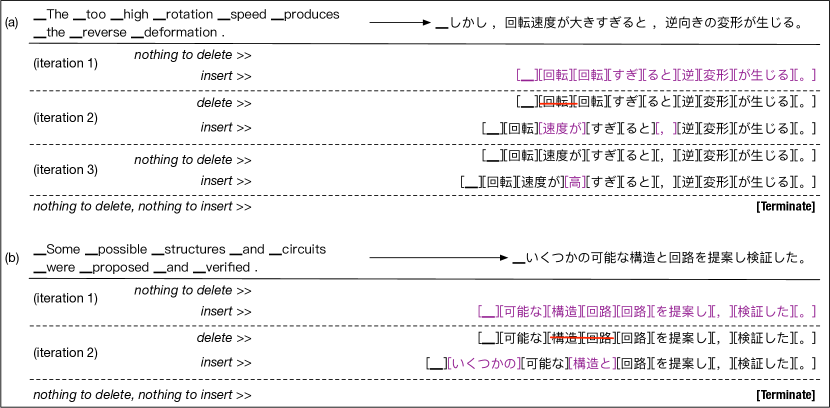
Figure 6: Translation examples for WAT’17 Small-NMT En-Ja with the Levenshtein Transformer.

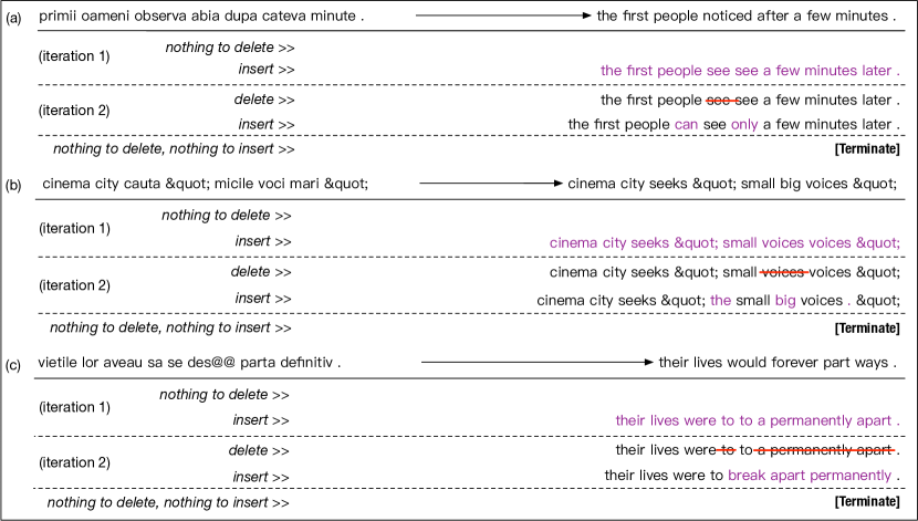
Figure 7: Translation examples for WMT’16 Ro-En with the Levenshtein Transformer.

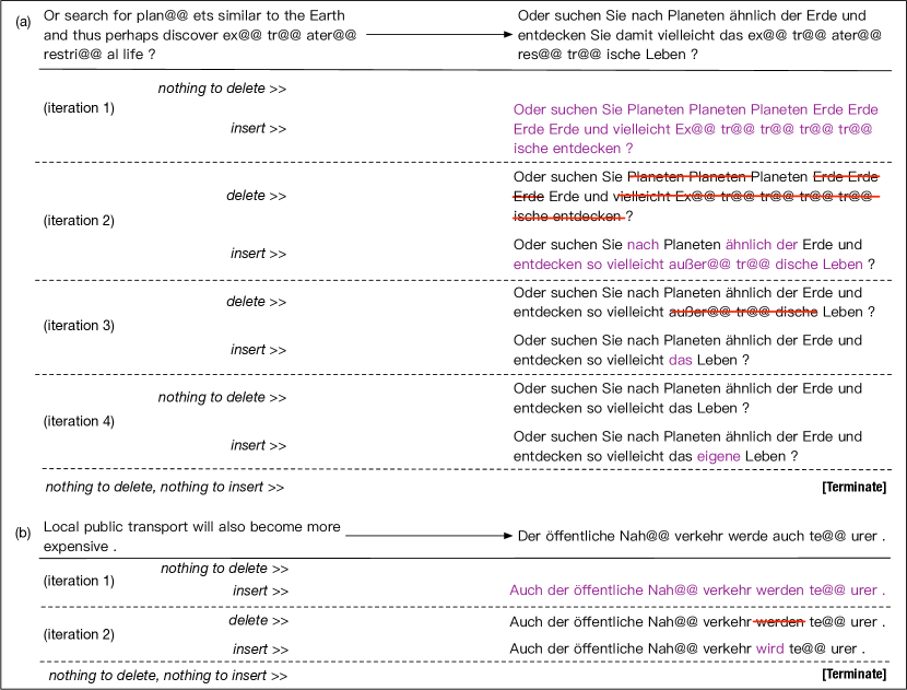
Figure 8: Translation examples for WMT’14 En-De with the Levenshtein Transformer.

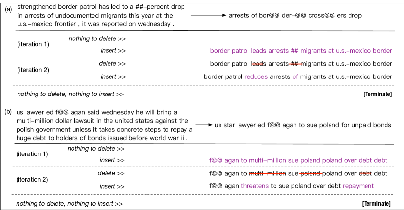
Figure 9: Translation examples for English Gigaword with the Levenshtein Transformer.

Figure 10: Post-editing examples for WMT’17-APE En-De with the Levenshtein Transformer.

Figure 11: An example for machine translation and zero-shot post-editing over a PBMT system’s output on WMT’16 Ro-En with the Levenshtein Transformer (LevT) trained for MT. It is clear to find that, the pre-trained LevT can directly adapt to the PBMT’s output and have a different refinement results compared to translate from scratch.

References

- Bahdanau et al. (2015) Dzmitry Bahdanau, Kyunghyun Cho, and Yoshua Bengio. 2015. Neural machine translation by jointly learning to align and translate. In 3rd International Conference on Learning Representations, ICLR 2015, San Diego, CA, USA, May 7-9, 2015, Conference Track Proceedings.
- Cho (2016) Kyunghyun Cho. 2016. Noisy parallel approximate decoding for conditional recurrent language model. arXiv preprint arXiv:1605.03835.
- Devlin et al. (2018) Jacob Devlin, Ming-Wei Chang, Kenton Lee, and Kristina Toutanova. 2018. BERT: pre-training of deep bidirectional transformers for language understanding. CoRR, abs/1810.04805.
- Dong et al. (2019) Yue Dong, Zichao Li, Mehdi Rezagholizadeh, and Jackie Chi Kit Cheung. 2019. Editnts: An neural programmer-interpreter model for sentence simplification through explicit editing. arXiv preprint arXiv:1906.08104.
- Freitag et al. (2019) Markus Freitag, Isaac Caswell, and Scott Roy. 2019. Text repair model for neural machine translation. arXiv preprint arXiv:1904.04790.
- Ghazvininejad et al. (2019) Marjan Ghazvininejad, Omer Levy, Yinhan Liu, and Luke Zettlemoyer. 2019. Constant-time machine translation with conditional masked language models. CoRR, abs/1904.09324.
- Goodfellow et al. (2014) Ian Goodfellow, Jean Pouget-Abadie, Mehdi Mirza, Bing Xu, David Warde-Farley, Sherjil Ozair, Aaron Courville, and Yoshua Bengio. 2014. Generative adversarial nets. In Advances in neural information processing systems, pages 2672–2680.
- Grangier and Auli (2017) David Grangier and Michael Auli. 2017. Quickedit: Editing text & translations by crossing words out. arXiv preprint arXiv:1711.04805.
- Gu et al. (2018) Jiatao Gu, James Bradbury, Caiming Xiong, Victor O.K. Li, and Richard Socher. 2018. Non-autoregressive neural machine translation. In 6th International Conference on Learning Representations, ICLR 2018, Vancouver, Canada, April 30-May 3, 2018, Conference Track Proceedings.
- Gu et al. (2019) Jiatao Gu, Qi Liu, and Kyunghyun Cho. 2019. Insertion-based decoding with automatically inferred generation order. arXiv preprint arXiv:1902.01370.
- Guu et al. (2018) Kelvin Guu, Tatsunori B Hashimoto, Yonatan Oren, and Percy Liang. 2018. Generating sentences by editing prototypes. Transactions of the Association of Computational Linguistics, 6:437–450.
- Kaiser et al. (2018) Lukasz Kaiser, Samy Bengio, Aurko Roy, Ashish Vaswani, Niki Parmar, Jakob Uszkoreit, and Noam Shazeer. 2018. Fast decoding in sequence models using discrete latent variables. In International Conference on Machine Learning, pages 2395–2404.
- Kim and Rush (2016) Yoon Kim and Alexander Rush. 2016. Sequence-level knowledge distillation. In EMNLP.
- Koehn et al. (2003) Philipp Koehn, Franz Josef Och, and Daniel Marcu. 2003. Statistical phrase-based translation. In Proceedings of the 2003 Conference of the North American Chapter of the Association for Computational Linguistics on Human Language Technology-Volume 1, pages 48–54. Association for Computational Linguistics.
- Lee et al. (2018) Jason Lee, Elman Mansimov, and Kyunghyun Cho. 2018. Deterministic non-autoregressive neural sequence modeling by iterative refinement. In Proceedings of the 2018 Conference on Empirical Methods in Natural Language Processing, Brussels, Belgium, October 31 - November 4, 2018, pages 1173–1182.
- Levenshtein (1965) Vladimir Iosifovich Levenshtein. 1965. Binary codes capable of correcting deletions, insertions, and reversals. In Doklady Akademii Nauk, volume 163, pages 845–848. Russian Academy of Sciences.
- Lin (2004) Chin-Yew Lin. 2004. Rouge: A package for automatic evaluation of summaries. In Text Summarization Branches Out: Proceedings of the ACL-04 Workshop, pages 74–81, Barcelona, Spain. Association for Computational Linguistics.
- Nakazawa et al. (2017) Toshiaki Nakazawa, Shohei Higashiyama, Chenchen Ding, Hideya Mino, Isao Goto, Hideto Kazawa, Yusuke Oda, Graham Neubig, and Sadao Kurohashi. 2017. Overview of the 4th workshop on Asian translation. In Proceedings of the 4th Workshop on Asian Translation (WAT2017), pages 1–54, Taipei, Taiwan. Asian Federation of Natural Language Processing.
- Novak et al. (2016) Roman Novak, Michael Auli, and David Grangier. 2016. Iterative refinement for machine translation. arXiv preprint arXiv:1610.06602.
- Papineni et al. (2002) Kishore Papineni, Salim Roukos, Todd Ward, and Wei-Jing Zhu. 2002. Bleu: a method for automatic evaluation of machine translation. In Proceedings of the 40th annual meeting on association for computational linguistics, pages 311–318. Association for Computational Linguistics.
- Rush et al. (2015) Alexander M. Rush, Sumit Chopra, and Jason Weston. 2015. A neural attention model for abstractive sentence summarization. In Proceedings of the 2015 Conference on Empirical Methods in Natural Language Processing, pages 379–389, Lisbon, Portugal. Association for Computational Linguistics.
- Sabour et al. (2018) Sara Sabour, William Chan, and Mohammad Norouzi. 2018. Optimal completion distillation for sequence learning. arXiv preprint arXiv:1810.01398.
- Sennrich et al. (2016) Rico Sennrich, Barry Haddow, and Alexandra Birch. 2016. Neural machine translation of rare words with subword units. In Proceedings of the 54th Annual Meeting of the Association for Computational Linguistics (Volume 1: Long Papers), pages 1715–1725, Berlin, Germany. Association for Computational Linguistics.
- Snover et al. (2006) Matthew Snover, Bonnie Dorr, Richard Schwartz, Linnea Micciulla, and John Makhoul. 2006. A study of translation edit rate with targeted human annotation. In In Proceedings of Association for Machine Translation in the Americas, pages 223–231.
- Stern et al. (2019) Mitchell Stern, William Chan, Jamie Kiros, and Jakob Uszkoreit. 2019. Insertion transformer: Flexible sequence generation via insertion operations. arXiv preprint arXiv:1902.03249.
- Stern et al. (2018) Mitchell Stern, Noam Shazeer, and Jakob Uszkoreit. 2018. Blockwise parallel decoding for deep autoregressive models. In Advances in Neural Information Processing Systems, pages 10107–10116.
- Vaswani et al. (2017) Ashish Vaswani, Noam Shazeer, Niki Parmar, Jakob Uszkoreit, Llion Jones, Aidan N. Gomez, Lukasz Kaiser, and Illia Polosukhin. 2017. Attention is all you need. In Proceedings of the Annual Conference on Neural Information Processing Systems (NIPS).
- Wang et al. (2018) Chunqi Wang, Ji Zhang, and Haiqing Chen. 2018. Semi-autoregressive neural machine translation. In Proceedings of the 2018 Conference on Empirical Methods in Natural Language Processing, pages 479–488, Brussels, Belgium. Association for Computational Linguistics.
- Welleck et al. (2019) Sean Welleck, Kianté Brantley, Hal Daumé III, and Kyunghyun Cho. 2019. Non-monotonic sequential text generation. arXiv preprint arXiv:1902.02192.
- Xia et al. (2017) Yingce Xia, Fei Tian, Lijun Wu, Jianxin Lin, Tao Qin, Nenghai Yu, and Tie-Yan Liu. 2017. Deliberation networks: Sequence generation beyond one-pass decoding. In Advances in Neural Information Processing Systems, pages 1784–1794.