Optimal dynamics of a spherical squirmer in Eulerian description

Abstract

The problem of optimization of a cycle of tangential deformations of the surface of a spherical object (microsquirmer) self-propelling in a viscous fluid at low Reynolds numbers is represented in a noncanonical Hamiltonian form. The evolution system of equations for the coefficients of expansion of the surface velocity in the associated Legendre polynomials $P^{1}_{n}(\cos\theta)$ is obtained. The system is quadratically nonlinear, but it is integrable in the three-mode approximation. This allows a theoretical interpretation of numerical results previously obtained for this problem.

Introduction

The hydrodynamics of swimming microorganisms has currently become a separate field of research at the interface between biology and mechanics (see review [1] and numerous references therein). In addition, this field is of interest for the creation of medical nanorobots. The aim of hydrodynamics in this application is the quantitative description of motion of a fluid and active objects in it. For their motion, microorganisms involve diverse tools and skills such as flagella, cilia, and surface deformations. The decisive simplification of the theory can be achieved because fluids flow at a very low Reynolds numbers [2], when effects of inertia are insignificant as compared to viscosity (Stokes regime). Consequently, the velocity field almost instantaneously and unambiguously responds to any change in the shape of a body, shifting it in space. It is important that the displacement of an object periodically varying its state can be nonzero in a cycle only in the presence of a “loop” in the space of parameters characterizing the shape of the body. Therefore, the number of such time-dependent parameters, i.e., internal degrees of freedom, should be no less than two. A number of proposed simplified models allowed the comprehensive study of the mechanics of viscous swimming. In particular, a “three-sphere swimmer” with two arms with a variable length is well known [3-6]. Other models, including much more complex ones, were also studied (see, e.g., [2, 7-10] and references therein). Another type of swimming occurs through tangential deformations of the surface of a body without changing its geometric shape [11-15]. Such a model microorganism is called squirmer. The simplest squirmer is spherical and allows a simple exact solution of the problem in terms of associated Legendre polynomials [11, 12]. More precisely, if the tangential velocity field in the coordinate system associated with the sphere is expanded in the series

$$u_{\theta}(\theta,t)=\sin\theta\sum_{n=1}^{\infty}\frac{a_{n}(t)P^{\prime}_{n}(\cos\theta)}{n(n+1)},$$ (1)

the velocity of the squirmer along its axis of symmetry with respect to the fluid at rest at infinity is $U_{\rm sq}(t)=a_{1}(t)/3$. Since the surface velocity $u_{\theta}(\theta,t)$ is determined by the motion of certain Lagrangian markers $\theta_{0}$,

$$u_{\theta}(\theta,t)=\frac{\partial\theta(\theta_{0},t)}{\partial t}\Big{|}_{\theta_{0}=\theta_{0}(\theta,t)}.$$ (2)

The time-periodic (bijective) mapping $\theta(\theta_{0},t)$ specifies the “loop” in the configuration space of the squirmer that is responsible for its locomotion.

Here, it is reasonable to immediately estimate the energy efficiency of any given cycle. If only the mechanical energy dissipation in the surrounding fluid is taken into account and internal energy consumptions are disregarded, the instantaneous dissipation rate is given by the expression

$$Q\propto\sum_{n}\frac{D_{n}}{2n+1}a_{n}^{2},$$ (3)

Here, $D_{1}=1$ and the other coefficients are specified by the formula [11, 12]

$$D_{n}=\frac{2n+1}{n(n+1)},\qquad n\geq 2.$$ (4)

Below, the general case of arbitrary coefficients $D_{n}>0$ is considered with particular numerical examples.

It is convenient to reformulate the problem of optimization of the cycle in other variables [16]. Let $x=\cos\theta$ be a Lagrangian mapping of the surface. Then, the corresponding velocity field has the form

$$v(x,t)=-\sin\theta u_{\theta}=\sum_{n=1}^{\infty}a_{n}(t)\Big{(}\frac{d}{dx}\Big{)}^{-1}P_{n}(x),$$ (5)

where

$$\Big{(}\frac{d}{dx}\Big{)}^{-1}P_{n}(x)=-\frac{(1-x^{2})P^{\prime}_{n}(x)}{n(n+1)}.$$ (6)

and

$$a_{n}(t)=-\frac{(2n+1)}{2}\int P^{\prime}_{n}(x)v(x,t)dx.$$ (7)

Correspondingly,

$$U_{\rm sq}(t)=\frac{a_{1}(t)}{3}=-\frac{1}{2}\int v(x,t)dx.$$ (8)

The optimal cycle should ensure the maximum displacement of the sphere in period at limited energy consumption. Such a cycle was found numerically in [16] in terms of the mapping $x(x_{0},t)$ by the gradient maximization of the ratio $\langle a_{1}\rangle^{2}/\langle Q\rangle$, where the angular brackets stand for averaging over the period. However, the time dependences of the coefficients $a_{n}(t)$ were obtained indirectly already after solving the equation of motion for $x(x_{0},t)$ . The interpretation of higher modes was rather difficult. In general, the analytical analysis of the problem remains incomplete.

The aim of this work is to supplement [16] by the theoretical analysis of the problem of optimization of a spherical squirmer taking into account the existing symmetry of redefinition of Lagrangian markers $x_{0}=x_{0}(\xi_{0})$. As will be shown below, the system of equations of motion for the problem can be obtained directly in terms of $a_{n}(t)$. Furthermore, these differential equations are only of the first order on time and are resolved with respect to the time derivative. Moreover, the three-mode approximation is integrable, thus completely revealing the structure of the corresponding solution.

Hamiltonian mechanics of optimization

It is convenient to use standard conservative dynamics. In view of Eq. (8), the most efficient cycle of the squirmer should ensure the minimum of the “action” functional $A=\int Ldt$ for the Lagrangian

$$L[v]=\int_{-1}^{1}\Big{(}\frac{1}{2}v\hat{D}v+\lambda v\Big{)}dx,\,\mbox{ where }v=-\frac{\partial x_{0}/\partial t}{\partial x_{0}/\partial x},$$ (9)

$\lambda$ is an indefinite Lagrange multiplier, and $\hat{D}$ is the operator specified as

$$\hat{D}v=-\sum_{k=1}^{\infty}D_{k}a_{k}(t)P^{\prime}_{k}(x).$$ (10)

The variation of the action with respect to $\delta x_{0}(x,t)$ easily gives the corresponding Euler-Lagrange dynamic equation. Simple algebra reduces this equation to the equation

$$\frac{\partial p}{\partial t}=-\frac{\partial}{\partial x}(vp)-p\frac{\partial v}{\partial x},$$ (11)

where $p(x,t)=\delta L[v]/\delta v$ is the canonical momentum. In our case,

$$p=\hat{D}v+\lambda.$$ (12)

It is noteworthy that the Lagrangian mapping itself is absent here and Eq. (11) is of the first order in the time derivative rather than of the second order. This is due to the mentioned symmetry of the redefinition when passing from the Lagrangian to Eulerian description.

Equation (11) has a noncanonical Hamiltonian structure. Under the standard definition of the Hamiltonian functional $H[p]$ as the Legendre transform of the Lagrangian $L[v]$, $v=\delta H/\delta p$ and Eq. (11) becomes

$$\frac{\partial p}{\partial t}=-\frac{\partial}{\partial x}\Big{(}p\frac{\delta H}{\delta p}\Big{)}-p\frac{\partial}{\partial x}\frac{\delta H}{\delta p}.$$ (13)

The variational principle $\delta\int{\cal L}dt=0$ for such dynamic systems has a somewhat unusual form

$${\cal L}=-\int\sqrt{p}\partial_{x}^{-1}\partial_{t}\sqrt{p}\,dx\,-H[p].$$ (14)

For any Hamiltonian, there is the law of conservation

$$\int\sqrt{p}\,dx=S=\mbox{const}.$$ (15)

The case where $p(x,t)$ is a sign-alternating function remains questionable.

Equations for the coefficients

The substitution of Eqs. (5) and (10) into Eq. (11), multiplication of the result by $(d/dx)^{-1}P_{m}(x)$, and integration over $x$ yield the infinite system of ordinary differential equations

$$\frac{2D_{m}}{2m+1}\dot{a}_{m}=2\lambda\sum_{n}\Omega_{mn}a_{n}+\sum_{n,k}W_{mnk}a_{n}D_{k}a_{k},$$ (16)

where the elements of the antisymmetric matrix $\Omega$ are given by the expression

$$\Omega_{mn}=-\Omega_{nm}=-\int_{-1}^{1}P_{n}(x)\Big{(}\frac{d}{dx}\Big{)}^{-1}P_{m}(x)dx.$$ (17)

In view of the properties of the Legendre polynomials, only the matrix elements between neighboring modes are nonzero; they are given by the formula

$$\Omega_{m,m-1}=\frac{2}{(2m+1)(2m-1)}.$$ (18)

The quadratic nonlinearity tensor W is also antisymmetric in its first two indices. After integration by parts, it is reduced to the form

$$W_{mnk}=\Big{[}\frac{1}{m(m+1)}-\frac{1}{n(n+1)}\Big{]}J_{mnk},$$ (19)

$$J_{mnk}=\int_{-1}^{1}(1-x^{2})P^{\prime}_{m}(x)P^{\prime}_{n}(x)P_{k}(x)dx.$$ (20)

Here, nonzero elements are obviously only those for which $m+n+k=2l$, where $l$ is an integer, and $(m+n)\geq k$. The first nonzero elements are $W_{1,2,1}=4/15$, $W_{1,2,3}=-4/35$, $W_{1,3,2}=2/7$, $W_{2,3,1}=4/35$, and $W_{2,3,3}=2/105$.

Since $\Omega$ and $W$ are antisymmetric, the dissipation rate on the optimal cycle is an integral of motion, i.e., constant in time:

$$\sum_{m}\frac{D_{m}}{2m+1}a_{m}^{2}=E=\mbox{const}.$$ (21)

Thus, motion occurs on an ellipsoid in the multidimensional phase space.

(a)

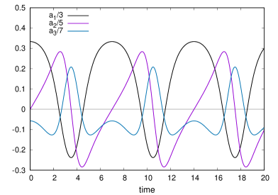
(b)

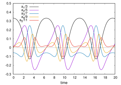
Figure 1: (a) Three- and (b) five-mode approximations.

Finite-mode approximations

The numerical results obtained in [16] indicate that the amplitudes $a_{n}$ on the optimal solution decrease exponentially with increasing number $n$. A finite-dimensional dynamic system obtained by setting $a_{n}=0$ at $n>N$ in Eqs. (16) is no longer Hamiltonian. The law of conservation given by Eq. (15) is also “violated.” However, such approximations can be useful if one finds their solutions such that highest modes carry only a small fraction of the total “energy.” In this context, the cases $N=3$ and $N=5$ are remarkable. The equations in the case $N=3$ have the form

$$\frac{2D_{1}}{3}\dot{a}_{1} = -\frac{4\lambda}{15}a_{2}+\frac{4}{15}a_{2}D_{1}a_{1}$$ (22)

$$- \frac{4}{35}a_{2}D_{3}a_{3}+\frac{2}{7}a_{3}D_{2}a_{2},$$

$$\frac{2D_{2}}{5}\dot{a}_{2} = \frac{4\lambda}{15}a_{1}-\frac{4\lambda}{35}a_{3}-\frac{4}{15}a_{1}D_{1}a_{1}$$ (23)

$$+ \frac{4}{35}a_{1}D_{3}a_{3}+\frac{4}{35}a_{3}D_{1}a_{1}+\frac{2}{105}a_{3}D_{3}a_{3},$$

$$\frac{2D_{3}}{7}\dot{a}_{3} = \frac{4\lambda}{35}a_{2}-\frac{2}{7}a_{1}D_{2}a_{2}$$ (24)

$$- \frac{4}{35}a_{2}D_{1}a_{1}-\frac{2}{105}a_{2}D_{3}a_{3}.$$

This system has an additional integral of motion $F(a_{1},a_{3})=C$, because the factor $a_{2}$ is common for all terms on the right-hand sides of Eqs. (22) and (24). Thus, the ratio of Eqs. (22) and (24) is free of the variable $a_{2}$ and corresponds to an autonomous linear inhomogeneous system with a focus singular point. The phase trajectory is the intersection of the ellipsoid given by Eq. (21) and a surface from the family $F(a_{1},a_{3})=C$ (it is assumed that the focus is beyond the ellipsoid). An example of the three-mode dynamics is shown in Fig. 1a. In the case $N=5$, initial conditions can be easily chosen such that the phase trajectory is nearly periodic and passes through relatively small $a_{4}$ and $a_{5}$ values, as shown in Fig. 1b. This picture is qualitatively very similar to Fig. 6 in [16]. However, Fig. 1b quantitatively presents a different optimal cycle because the action functional really has many local minima, as mentioned by the authors of [16].

An algorithm for numerically seeking appropriate periodic solutions for systems with $N>5$ has not yet been developed. The trial-and-error method gave no results for such systems.

It should be emphasized that the problem of optimization does not end with solving the dynamic system given by Eq. (16). Further, it is necessary to select solutions on which the displacement is really maximal. However, some slightly nonoptimal solutions can be preferable under additional constraints on the properties of Lagrangian mappings. For example, if the most optimal solution dictates overly large displacements of Lagrangian markers in the angle $\theta$ that are impossible according to the internal structure of a real squirmer, solutions with a smaller amplitude can be considered.

Conclusions

To summarize, the Eulerian description of the optimal dynamics of the spherical squirmer has revealed its noncanonical Hamiltonian structure. Furthermore, within this description, equations of motion convenient for numerical solution have been derived directly in terms of the coefficients of expansion of the velocity field on the surface. The found approximate solutions and their arrangement in the phase space make it possible to better understand the behavior of several most important first modes.

A similar approach can also be used for other axisymmetric squirmers, but the velocity field $v(x,t)$ should be expanded in appropriate sets of functions depending on the geometrical shape of an object.

References

- (1) E. Lauga and T. R. Powers, Rep. Prog. Phys. 72, 096601 (2009).
- (2) E. M. Purcell, Am. J. Phys. 45, 3 (1977).
- (3) A. Najafi and R. Golestanian, Phys. Rev. E 69, 062901 (2004);
- (4) R. Golestanian and A. Ajdari, Phys. Rev. E 77, 036308 (2008).
- (5) F. Alouges, A. DeSimone, and A. Lefebvre, Eur. Phys. J. E 28, 279 (2009).
- (6) R. Zargar, A. Najafi, and M. Miri, Phys. Rev. E 80, 026308 (2009).
- (7) J. E. Avron, O. Gat, and O. Kenneth, Phys. Rev. Lett. 93, 186001 (2004).
- (8) E. Gauger and H. Stark, Phys. Rev. E 74, 021907 (2006).
- (9) D. Tam and A. E. Hosoi, Phys. Rev. Lett. 98, 068105 (2007).
- (10) D. Takagi, Phys. Rev. E 92, 023020 (2015).
- (11) M. J. Lighthill, Commun. Pure Appl. Math. 5, 109 (1952).
- (12) J. R. Blake, J. Fluid Mech. 46, 199 (1971).
- (13) O. S. Pak and E. Lauga, J. Eng. Math. 88, 1 (2014).
- (14) M. Theers, E. Westphal, G. Gompper, and R. G. Winkler, Soft Matter 12, 7372 (2016).
- (15) D. Papavassiliou and G. P. Alexander, J. Fluid Mech. 813, 618 (2017)
- (16) S. Michelin and E. Lauga, Physics of Fluids 22, 111901 (2010).