Graph Filtration Learning

Abstract

We propose an approach to learning with graph-structured data in the problem domain of graph classification. In particular, we present a novel type of readout operation to aggregate node features into a graph-level representation. To this end, we leverage persistent homology computed via a real-valued, learnable, filter function. We establish the theoretical foundation for differentiating through the persistent homology computation. Empirically, we show that this type of readout operation compares favorably to previous techniques, especially when the graph connectivity structure is informative for the learning problem.

1 Introduction

We consider the task of learning a function from the space of (finite) undirected graphs, $\mathbb{G}$, to a (discrete/continuous) target domain $\mathbb{Y}$. Additionally, graphs might have discrete, or continuous attributes attached to each node. Prominent examples for this class of learning problem appear in the context of classifying molecule structures, chemical compounds or social networks.

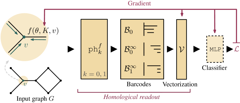
Figure 1: Overview of the proposed homological readout. Given a graph/simplicial complex, we use a vertex-based graph functional $f$ to assign a real-valued score to each node. A practical choice is to implement $f$ as a GNN, with one level of message passing. We then compute persistence barcodes, $\mathcal{B}_{k}$, using the filtration induced by $f$. Finally, barcodes are fed through a vectorization scheme $\mathcal{V}$ and passed to a classifier (e.g., an MLP). Our approach allows passing a learning signal through the persistent homology computation, allowing to optimize $f$ for the classification task.

A substantial amount of research has been devoted to developing techniques for supervised learning with graph-structured data, ranging from kernel-based methods (Shervashidze et al., 2009, 2011; Feragen et al., 2013; Kriege et al., 2016), to more recent approaches based on graph neural networks (GNN) (Scarselli et al., 2009; Hamilton et al., 2017; Zhang et al., 2018b; Morris et al., 2019; Xu et al., 2019; Ying et al., 2018). Most of the latter works use an iterative message passing scheme (Gilmer et al., 2017) to learn node representations, followed by a graph-level pooling operation that aggregates node-level features. This aggregation step is typically referred to as a readout operation. While research has mostly focused on variants of the message passing function, the readout step may have a significant impact, as it aims to capture properties of the entire graph. Importantly, both simple and more refined readout operations, such as summation, differentiable pooling (Ying et al., 2018), or sort pooling (Zhang et al., 2018a), are inherently coupled to the amount of information carried over via multiple rounds of message passing. Hence, architectural GNN choices are typically guided by dataset characteristics, e.g., requiring to tune the number of message passing rounds to the expected size of graphs.

Contribution. We propose a homological readout operation that captures the full global structure of a graph, while relying only on node representations learned from immediate neighbors. This not only alleviates the aforementioned design challenge, but potentially offers additional discriminative information. Similar to previous works, we consider a graph, $G$, as a simplicial complex, $K$, and use persistent homology (Edelsbrunner & Harer, 2010) to capture homological changes that occur when constructing the graph one part at a time (i.e., revealing changes in the number of connected components or loops). As this hinges on an ordering of the parts, prior works rely on a suitable filter function $f:K\rightarrow\mathbb{R}$ to establish this ordering. Our idea differs in that we learn the filter function (end-to-end), as opposed to defining it a-priori) .

2 Related work

Graph neural networks. Most work on neural network based approaches to learning with graph-structured data focuses on learning informative node embeddings to solve tasks such as link prediction (Schütt et al., 2017), node classification (Hamilton et al., 2017), or classifying entire graphs. Many of these approaches, including (Scarselli et al., 2009; Duvenaud et al., 2015; Li et al., 2016; Battaglia et al., 2016; Kearns et al., 2016; Morris et al., 2019), can be formulated as a message passing scheme (Gilmer et al., 2017; Xu et al., 2018) where features of graph nodes are passed to immediate neighbors via a differentiable message passing function; this operation proceeds over multiple iterations with each iteration parameterized by a neural network. Aspects distinguishing these approaches include (1) the particular realization of the message passing function, (2) the way information is aggregated at the nodes, and (3) whether edge features are included. Due to the algorithmic similarity of iterative message passing and aggregation to the Weisfeiler-Lehman (WL) graph isomorphism test (Weisfeiler & Lehman, 1968), several works (Xu et al., 2019; Morris et al., 2019) have recently studied this connection and established a theoretical underpinning for analyzing properties of GNN variants in the context of the WL test.

Readout operations. With few exceptions, surprisingly little effort has been devoted to the so called readout operation, i.e., a function that aggregates node features into a global graph representation and allows making predictions for an entire graph. Common strategies include summation (Duvenaud et al., 2015), averaging, or passing node features through a network operating on sets (Li et al., 2016; Gilmer et al., 2017). As pointed out in (Ying et al., 2018), this effectively ignores the often complex global hierarchical structure of graphs. To mitigate this issue, (Ying et al., 2018) proposed a differentiable pooling operation that interleaves each message passing iteration and successively coarsens the graph. A different pooling scheme is proposed in (Zhang et al., 2018a), relying on appropriately sorting node features obtained from each message passing iteration. Both pooling mechanisms are generic and show improvements on multiple benchmarks. Yet, gains inherently depend on multiple rounds of message passing, as the global structure is successively captured during this process. In our alternative approach, global structural information is captured even initially. It only hinges on attaching a real value to each node which is learnably implemented via a GNN in one round of message passing.

Persistent homology & graphs. Notably, analyzing graphs via persistent homology is not new, with several works showing promising results on graph classification (Hofer et al., 2017; Carrière et al., 2019; Rieck et al., 2019b; Zhao & Wang, 2019). So far, however, persistent homology is used in a passive manner, meaning that the function $f$ mapping simplices to $\mathbb{R}$ is fixed and not informed by the learning task. Essentially, this degrades persistent homology to a feature extraction step, where the obtained topological summaries are fed through a vectorization scheme and then passed to a classifier. The success of these methods inherently hinges on the choice of the a-priori defined function $f$, e.g., the node degree function in (Hofer et al., 2017) or a heat kernel function in (Carrière et al., 2019). The difference to our approach is that backpropagating the learning signal stops at the persistent homology computation; in our case, the signal is passed through, allowing to adjust $f$ during learning.

3 Background

We are interested in describing graphs in terms of their topological features, such as connected components and cycles. Persistent homology, a method from computational topology, makes it possible to compute these features efficiently. Next, we provide a concise introduction to the necessary concepts of persistent homology and refer the reader to (Hatcher, 2002; Edelsbrunner & Harer, 2010) for details.

Homology. The key concept of homology theory is to study properties of an object $X$, such as a graph, by means of (commutative) algebra. Specifically, we assign to $X$ a sequence of groups/modules $C_{0},\ C_{1},\ldots$ which are connected by homomorphisms $\partial_{k+1}:C_{k+1}\rightarrow C_{k}$ such that $\operatorname{im}\partial_{k+1}\subseteq\ker\partial_{k}$. A structure of this form is called a chain complex and by studying its homology groups

$$H_{k}=\ker\partial_{k}/\operatorname{im}\partial_{k+1}$$ (1)

we can derive (homological) properties of $X$. The original motivation for homology is to analyze topological spaces. In that case, the ranks of homology groups yield directly interpretable properties, e.g., $\operatorname{rank}(H_{0})$ reflects the number of connected components and $\operatorname{rank}(H_{1})$ the number of loops.

A prominent example of a homology theory is simplicial homology. A simplicial complex, $K$, over the vertex domain $\mathbb{V}$ is a set of non-empty (finite) subsets of $\mathbb{V}$ that is closed under the operation of taking non-empty subsets and does not contain $\emptyset$. Formally, this means $K\subset\mathcal{P}(\mathbb{V})$ with $\sigma\in K\Rightarrow 1\leq|\sigma|<\infty$ and $\tau\subseteq\sigma\in K\Rightarrow\tau\in K$. We call $\sigma\in K$ a $k-$simplex iff $\dim(\sigma)=|\sigma|-1=k$; correspondingly $\dim(K)=\max_{\sigma\in K}\dim(\sigma)$ and we set $K_{k}=\{\sigma\in K:\dim(\sigma)=k\}$. Further, let $C_{k}(K)$ be the vector space generated by $K_{k}$ over $\mathbb{Z}/2\mathbb{Z}$ and define

$$\partial_{k}:K_{k}\rightarrow C_{k-1}(K)\quad\sigma\mapsto\sum\limits_{\begin{subarray}{c}\tau:\tau\subset\sigma\\ \dim(\tau)=k-1\end{subarray}}\tau\enspace.$$

In other words, $\sigma$ is mapped to the formal sum of its $(k-1)$-dim. faces, i.e., its subsets of cardinality $k$. The linear extension to $C_{k}(K)$ of this mapping defines the $k$-th boundary operator

$$\partial_{k}:C_{k}(K) \to C_{k-1}(K)$$

$$\sum\limits_{i=1}^{n}\sigma_{i} \mapsto\sum\limits_{i=1}^{n}\partial_{k}(\sigma_{i})\enspace.$$

Using $\partial_{k}$, we obtain the corresponding $k$-th homology group, $H_{k}$, as in Eq. (1).

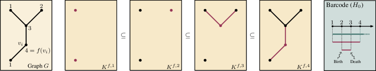
Figure 2: Illustration of $0$-dimensional persistent homology on a graph $G$, via a node-based filter function $f$. The barcode (shown right), computed by persistent homology is $\mathcal{B}_{0}=\{(1,4),(2,3)\}$. If we consider essential topological features, we further get $\mathcal{B}_{0}^{\infty}=\{1\}$.

Graphs are simplicial complexes. In fact, we can directly interpret a graph $G$ as an $1$-dimensional simplicial complex whose vertices ($0$-simplices) are the graphs nodes and whose edges ($1$-simplices) are the graphs edges. In this setting, only the 1 boundary operator is non trivial and simply maps an edge to the formal sum of its defining nodes. Via homology we can then compute the graph’s $0$ and $1$ dimensional topological features, i.e., connected components and cycles. However, as mentioned earlier, this only gives a rather coarse summary of the graph’s topological properties, raising the demand for a refinement of homology.

Persistent homology. For consistency with the relevant literature, we introduce the idea of refining homology to persistent homology in terms of simplicial complexes, but recall that graphs are $1$-dimensional simplicial complexes.

Now, let $(K^{i})_{i=0}^{m}$ be a sequence of simplicial complexes such that $\emptyset=K^{0}\subseteq K^{1}\subseteq\dots\subseteq K^{m}=K$. Then, $(K^{i})_{i=0}^{m}$ is called a filtration of $K$. Using the extra information provided by the filtration of $K$, we obtain a sequence of chain complexes where $C_{k}^{i}=C_{k}(K_{k}^{i})$ and $\iota$ denotes the inclusion. This leads to the concept of persistent homology groups, i.e.,

$$H_{k}^{i,j}=\ker\partial_{k}^{i}/(\operatorname{im}\partial_{k+1}^{j}\cap\ker\partial_{k}^{i})\quad\text{for}\quad 1\leq i\leq j\leq m\enspace.$$

The ranks, $\beta_{k}^{i,j}=\operatorname{rank}H_{k}^{i,j}$, of these homology groups (i.e., the $k$-th persistent Betti numbers), capture the number of homological features of dimensionality $k$ (e.g., connected components for $k=0$, loops for $k=1$, etc.) that persist from $i$ to (at least) $j$. According to the Fundamental Lemma of Persistent Homology (Edelsbrunner & Harer, 2010), the quantities

$$\mu_{k}^{i,j}=(\beta_{k}^{i,j-1}-\beta_{k}^{i,j})-(\beta_{k}^{i-1,j-1}-\beta_{k}^{i-1,j})$$ (2)

for $1\leq i<j\leq m$ encode all the information about the persistent Betti numbers of dimension $k$.

Persistence barcodes. In principle, introducing persistence barcodes only requires a filtration as defined above. In our setting, we define a filtration of $K$ via a vertex filter function $f:\mathbb{V}\rightarrow\mathbb{R}$. In particular, given the sorted sequence of filter values $a_{1}<\cdots<a_{m}$, i.e., $a_{i}\in\{f(v):\{v\}\in K_{0}\}$, we define the filtration w.r.t.$f$ as

$$\begin{split}K^{f,0}&=\emptyset\\ K^{f,i}&=\{\sigma\in K:\max\limits_{v\in\sigma}f(v)\leq a_{i}\}\\ \end{split}$$ (3)

for $1\leq i\leq m$. Intuitively, this means that the filter function is defined on the vertices of $K$ and lifted to higher dimensional simplices in $K$ by maximum aggregation. This enables us to consider a sub levelset filtration of $K$.

Then, for a given filtration of $K$ and $0\leq k\leq\dim(K)$, we can construct a multiset by inserting the point $(a_{i},a_{j})$, $1\leq i<j\leq m$, with multiplicity $\mu_{k}^{i,j}$. This effectively encodes the $k$-dimensional persistent homology of $K$ w.r.t. the given filtration. This representation is called a persistence barcode, $\mathcal{B}_{k}$. Hence, for a given complex $K$ of dimension $\dim(K)$ and a filter function $f$ (of the discussed form), we can interpret $k$-dimensional persistent homology as a mapping of simplicial complexes, defined by

$$\texttt{ph}_{k}^{f}(K)=\mathcal{B}_{k}\quad 0\leq k\leq\text{dim}(K)\enspace.$$ (4)

Remark 1.

By setting

$$\mu_{k}^{i,\infty}=\beta_{n}^{i,m}-\beta_{n}^{i-1,m}\enspace$$

we extend Eq. (2) to features which never disappear, also referred to as essential. If we use this extension, Eq. (4) yields an additional barcode, denoted as $\mathcal{B}_{k}^{\infty}$, per dimension. For practical reasons, the points in $\mathcal{B}_{k}^{\infty}$ are just the birth-time, as all death-times equal to $\infty$ and thus are omitted.

Persistent homology on graphs. In the setting of graph classification, we can think of a filtration as a growth process of a weighted graph. As the graph grows, we track homological changes and gather this information in its 0- and 1-dimensional persistence barcodes. An illustration of $0$-dimensional persistent homology for a toy graph example is shown in Fig. 2.

4 Filtration learning

Having introduced the required terminology, we now focus on the main contribution of this paper, i.e., how to learn an appropriate filter function. To the best of our knowledge, our paper constitutes the first approach to this problem. While different filter functions for graphs have been proposed and used in the past, e.g., based on degrees (Hofer et al., 2017), cliques (Petri et al., 2013), multiset distances (Rieck et al., 2019a), or the Jaccard distance (Zhao & Wang, 2019), prior work typically treats the filter function as fixed. In this setting, the filter function needs to be selected via, e.g., cross-validation, which is cumbersome. Instead, we show that it is possible to learn a filter function end-to-end.

This endeavor hinges on the capability of backpropagating gradients through the persistent homology computation. While this has previously been done in (Chen et al., 2019) or (Hofer et al., 2019b), their results are not directly applicable here, due to the special problem settings considered in these works. In (Chen et al., 2019), the authors regularize decision boundaries of classifiers, in (Hofer et al., 2019b) the authors impose certain topological properties on representations learned by an autoencoder. This warrants a detailed analysis in the context of graphs.

We start by recalling that the computation of sublevel set persistent homology, cf. Eq. (3), depends on two arguments: (1) the complex $K$ and (2) the filter function $f$ which determines the order of the simplices in the filtration of $K$. As $K$ is of discrete nature, it is clear that $K$ cannot be subject to gradient-based optimization. However, assume that the filter $f$ has a differentiable dependence on a real-valued parameter $\theta$. In this case, the persistent homology of the sublevel set filtration of $K$ also depends on $\theta$, raising the following question: Is the mapping differentiable in $\theta$?

Notation. If any symbol introduced in the context of persistent homology is dependent on $\theta$, we interpret it as function of $\theta$ and attach “$(\theta)$” to this symbol. If the dependence on the simplicial complex $K$ is irrelevant to the current context, we omit it for brevity. For example, we write $\mu_{k}^{i,j}(\theta)$ for the multiplicity of barcode points.

Next, we concretize the idea of a learnable vertex filter.

Definition 1 (Learnable vertex filter function).

Let $\mathbb{V}$ be a vertex domain, $\mathbb{K}$ the set of possible simplicial complexes over $\mathbb{V}$ and let

$$f:\mathbb{R}\times\mathbb{K}\times\mathbb{V}\rightarrow\mathbb{R}\quad\quad(\theta,K,v)\mapsto f(\theta,K,v)$$

be differentiable in $\theta$ for $K\in\mathbb{K},v\in\mathbb{V}$. Then, we call $f$ a learnable vertex filter function with parameter $\theta$.

The assumption that $f$ is dependent on a single parameter is solely dedicated to simplify the following theoretical part. The derived results immediately generalize to the case $f:\mathbb{R}^{n}\times\mathbb{K}\times\mathbb{V}$ where $n$ is the number of parameters and we will drop this assumption later on.

By Eq. (4), $(\theta,K)\mapsto\texttt{ph}_{k}^{f}(\theta,K)$ is a mapping to the space of persistence barcodes $\mathbb{B}$ (or $\mathbb{B}^{2}$ if essential barcodes are included). As $\mathbb{B}$ has no natural linear structure, we consider differentiability in combination with a coordinatization strategy $\mathcal{V}:\mathbb{B}\rightarrow\mathbb{R}$. This allows studying the map

$$(\theta,K)\mapsto\mathcal{V}\big{(}\texttt{ph}_{k}^{f}(\theta,K)\big{)}$$

for which differentiability is defined. In fact, we can rely on prior works on learnable vectorization schemes for persistence barcodes (Hofer et al., 2019a; Carrière et al., 2019). In the following definition of a barcode coordinate function, we adhere to (Hofer et al., 2019b).

Definition 2 (Barcode coordinate function).

Let $s:\mathbb{R}^{2}\rightarrow\mathbb{R}$ be a differentiable function that vanishes on the diagonal of $\mathbb{R}^{2}$. Then

$$\mathcal{V}:\mathbb{B}\rightarrow\mathbb{R}\quad\quad\mathcal{B}\mapsto\sum\limits_{(b,d)\in\mathcal{B}}s(b,d)$$

is called barcode coordinate function.

Intuitively, $\mathcal{V}$ maps a barcode $\mathcal{B}$ to a real value by aggregating the points in $\mathcal{B}$ via a weighted sum. Notably, the deep sets approach of (Zaheer et al., 2017) would also be a natural choice, however, not specifically tailored to persistence barcodes. Upon using $d$ barcode coordinate functions of the form described in Definition 2, we can effectively map a barcode into $\mathbb{R}^{d}$ and feed this representation through any differentiable layer downstream, e.g., implementing a classifier. We will discuss our particular choice of $s$ in §5.

Next, we show that, under certain conditions, $\texttt{ph}_{k}^{f}$ in combination with a suitable barcode coordinate function preserves differentiability. This is the key result that will enable end-to-end learning of a filter function.

Lemma 1.

Let $K$ be a finite simplicial complex with vertex set $V=\{v_{1},\dots,v_{n}\}$, $f:\mathbb{R}\times\mathbb{K}\times\mathbb{V}\rightarrow\mathbb{R}$ be a learnable vertex filter function as in Definition 1 and $\mathcal{V}$ a barcode coordinate function as in Definition 2. If, for $\theta_{0}\in\mathbb{R}$, it holds that the pairwise vertex filter values are distinct, i.e.,

$$f(\theta_{0},K,v_{i})\neq f(\theta_{0},K,v_{j})\quad\text{ for }\quad 1\leq i<j\leq n$$

then the mapping

$$\theta\mapsto\mathcal{V}\big{(}\texttt{ph}_{k}^{f}(\theta,K)\big{)}$$ (5)

is differentiable at $\theta_{0}$.

For brevity, we only sketch the proof; the full version can be found in the supplementary material.

Sketch of proof.

The pairwise vertex filter values

$$Y=\{f(\theta_{0},K,v_{i})\}_{i=1}^{n}$$

are distinct which implies that they are (P1) strictly ordered by “$<$” and (P2) $m=|Y|=n$. A cornerstone for the actual persistence computation is the index permutation $\pi$ which sorts $Y$. Now consider for some $h\in\mathbb{R}$ the set of vertex filter values for $\theta_{0}$ shifted by $h$, i.e., $Y^{\prime}=\{f(\theta_{0}+h,K,v_{i})\}_{i=1}^{n}$. Since $f$ is assumed to be differentiable, and therefore continuous, $Y^{\prime}$ also satisfies (P1) and (P2) and $\pi$ sorts $Y^{\prime}$, for $|h|$ sufficiently small. Importantly, this also implies

$$\big{(}K_{i}^{f}(\theta_{0})\big{)}_{i=0}^{n}=\big{(}K_{i}^{f}(\theta_{0}+h)\big{)}_{i=0}^{n}$$ (6)

and thus

$$\mu_{k}^{i,j}(\theta_{0})=\mu_{k}^{i,j}(\theta_{0}+h)\leavevmode\nobreak\ \text{for}\leavevmode\nobreak\ 1\leq i<j\leq n\enspace.$$ (7)

As a consequence, this allows deriving the equality

$$\lim\limits_{|h|\rightarrow 0}\frac{\mathcal{V}(\texttt{ph}_{k}^{f}(K,\theta_{0}))-\mathcal{V}(\texttt{ph}_{k}^{f}(K,\theta_{0}+h))}{h}$$

$$=$$

$$\sum\limits_{i<j}\mu_{k}^{i,j}(\theta_{0})\cdot\frac{\partial s\big{(}f(\theta,K,v_{\pi(i)}),f(\theta,K,v_{\pi(j)})\big{)}}{\partial\theta}(\theta_{0})\enspace.$$

This concludes the proof, since the derivative within the summation on the right exists (as $f$ was assumed to be differentiable). ∎

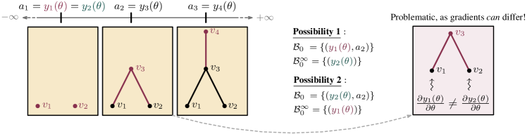
Figure 3: Illustration of a problematic scenario that can occur when trying to backpropagate through the persistent homology computation. The left-hand side shows three steps in a filtration sequence with filtration values $a_{i}=y_{i}(\theta)=f(\theta,K,v_{i})$, including the two valid choices of the $0$-dimensional barcode $\mathcal{B}_{0}$ and $\mathcal{B}_{0}^{\infty}$ (essential). Numerically, the barcodes for both choices are equal, however, depending on the tie settling strategy, the gradients may differ.

Analysis of Lemma 1. A crucial assumption in Lemma 1 is that the filtration values are pairwise distinct. If this is not the case, the sorting permutation $\pi$ is not uniquely defined and Eq. (7) does not hold. Although the gradient w.r.t. $\theta$ is still computable in this situation, it depends on the particular implementation of the persistent homology algorithm. The reason for this is that the latter depends on a strict total ordering of the simplices such that $\tau<\sigma$ whenever $\tau$ is a face of $\sigma$, formally $\tau\in\{\rho\subseteq\sigma:\dim\rho=\dim\sigma-1\}\Rightarrow\tau<\sigma$. Specifically, the sublevel set filtration $(K^{f,i})_{i=1}^{m}$, only yields a partial strict ordering by

$$\sigma\in K_{i},\tau\in K_{j}\quad\text{and}\quad i<j \Rightarrow\sigma<\tau\enspace,$$ (8)

$$\sigma,\tau\in K_{i}\quad\text{and}\quad\dim(\sigma)<\dim(\tau) \Rightarrow\sigma<\tau\enspace.$$ (9)

However, in the case

$$\sigma,\tau\in K_{i}\land\dim(\sigma)=\dim(\tau)$$

we can neither infer $\sigma<\tau$ nor $\sigma>\tau$ from Eq. (8) and Eq. (9). Hence, those “ties” need to be settled in the implementation. If we were only interested in the barcodes, the tie settling strategy would be irrelevant as the barcodes do not depend on the implementation. To see this, consider a point $(a,b)$ in the barcode $\mathcal{B}$. Now let

$$I_{a} =\{i:1\leq{}i\leq n,f(\theta,K,v_{i})=a\},\text{ and}$$

$$I_{b} =\{i:1\leq i\leq n,f(\theta,K,v_{i})=b\}\enspace.$$

Then, if $|I_{a}|>1$ or $|I_{b}|>1$ the representation of $(a,b)\in\mathcal{B}$ may not be unique but dependent on the tie settling strategy used in the implementation of persistent homology. In this case, the particular choice of tie settling strategy, could affect the gradient. In Fig. 3, we illustrate this issue on a toy example of a problematic configuration. Conclusively, different implementations yield the same barcodes, but probably different gradients.

Remark 2.

An alternative, but computationally more expensive, strategy would be as follows: for a particular filtration value $a$, let $I_{a}=\{i:1\leq i\leq n,f(\theta,K,v_{i})=a\}$. Now consider a point $(a,b)$ in the barcode with a “problematic” configuration, cf. Fig. 3 in $a$. Upon setting

$$(a,b)=\big{(}\nicefrac{{1}}{{|I_{a}|}}\sum_{i\in I_{a}}f(\theta,K,v_{i}),b\big{)}\enspace,$$

i.e., the (mean) aggregation of all possible representations of $(a,b)$, this results in a gradient which is independent of the actual tie settling strategy. Yet, this is far more expensive to compute, due to the index set construction of $I_{a}$, especially if $n$ is large. While it can be argued that this strategy is more “natural“, it would lead to a more involved proof for differentiability, which we leave for future work.

The difficulty of assigning/defining a proper gradient if the filtration values are not pairwise distinct is not unique to our approach. In fact, other set operations frequently used in neural networks face a similar problem. For example, consider the popular maxpool operator $\{y_{1},\dots,y_{n}\}\mapsto\max(\{y_{1},\dots,y_{n}\})=z$, which is a well defined mapping. However, in the case of, say, $z=y_{1}=y_{2}$, it is unclear if $y_{1}$ or $y_{2}$ is used to represent its value $z$. In the situation of $z=y_{1}=\varphi_{\theta}(x_{1})=y_{2}=\varphi_{\theta}(x_{2})$ for some differentiable function $\varphi_{\theta}$, with differing gradients (w.r.t. $\theta$) at $x_{1}$ and $x_{2}$ this could be problematic. In fact, the gradient w.r.t. $\theta$ would then depend on the particular choice of representing $z$, i.e., the particular implementation of the maxpool operator.

4.1 Graph filtration learning (GFL)

Having established the theoretical foundation of our approach, we now describe its practical application to graphs. First note that, as briefly discussed in §3, graphs are simplicial complexes, although they are notationally represented in slightly different ways. For a graph $G=(V,E)$ we can directly define its simplicial complex by $K_{G}=\big{\{}\{v\}:v\in V\big{\}}\cup E$. We ignore this notational nuance and use $G$ and $K_{G}$ interchangeably. In fact, learning filtrations on graph-structured data integrates seamlessly into the presented framework. Specifically, the learnable vertex filter function, generically introduced in Definition 1, can be easily implemented by a neural network. If local node neighborhood information should be taken into account, this can be realized via a graph neural network (GNN; see Wu et al. (2020) for a comprehensive survey), operating on an initial node representation $l:\mathbb{V}\to\mathbb{R}^{n}$. The learnable vertex filter function then is a mapping of the form $v\mapsto\texttt{GNN}(G,l(v))$.

Selection of $\mathcal{V}$. We use a vectorization based on a local weighting function, $s:\mathbb{R}^{2}\rightarrow\mathbb{R}$, of points in a given barcode, $\mathcal{B}$. In particular, we select the rational hat structure element of (Hofer et al., 2019b), which is of the form

$$\mathcal{B}\ni p\mapsto\frac{1}{1+\|p-c\|_{1}}-\frac{1}{1+\big{|}|r|-\|p-c\|_{1}\big{|}}\enspace,$$ (10)

where $c\in\mathbb{R}^{2},r\in\mathbb{R}$ are learnable parameters. Intuitively, this can be seen as a function that evaluates the “centrality” of each point $p$ of the barcode $\mathcal{B}$ w.r.t.  a learnt center $c$ and a learnt shift/radius $r$. The reason we prefer this variant over alternatives is that it yields a rational dependency w.r.t. $c$ and $r$, resulting in tamer gradient behavior during optimization. This is even more critical as, different to (Hofer et al., 2019b), we optimize over parts of the model which appear before $\mathcal{V}$ and are thus directly dependent on its gradient.

We remark that our approach is not specifically bound to the choice in Eq. (10). In fact, one could possibly use the strategies proposed by Carrière et al. (2019) or Zhao & Wang (2019) and we do not claim that our choice is optimal in any sense.

Method	REDDIT-BINARY	REDDIT-MULTI-5K	IMDB-BINARY	IMDB-MULTI
	Initial node features: uninformative		Initial node features: $l(v)=\deg(v)$
PH-only	$90.3_{\pm 2.6}$	$55.7_{\pm 2.1}$	$68.9_{\pm 3.5}$	$46.1_{\pm 4.2}$
1-GIN (GFL)	$90.2_{\pm 2.8}$	$55.7_{\pm 2.9}$	$74.5_{\pm 4.6}$	$49.7_{\pm 2.9}$
1-GIN (SUM) (Xu et al., 2019)	$81.2_{\pm 5.4}$	$51.0_{\pm 2.2}$	$73.5_{\pm 3.8}$	$50.3_{\pm 2.6}$
1-GIN (SP) (Zhang et al., 2018a)	$76.8_{\pm 3.6}$	$48.5_{\pm 1.8}$	$73.0_{\pm 4.0}$	$50.5_{\pm 2.1}$
Baseline (Zaheer et al., 2017)	$77.5_{\pm 4.2}$	$45.7_{\pm 1.4}$	$72.7_{\pm 4.6}$	$49.9_{\pm 4.0}$
State-of-the-Art (NN)
DCNN (Wang et al., 2018)	n/a	n/a	$49.1$	$33.5$
PatchySAN (Niepert et al., 2016)	$86.3$	$49.1$	$71.0$	$45.2$
DGCNN (Zhang et al., 2018a)	n/a	n/a	$70.0$	$47.8$
1-2-3-GNN (Morris et al., 2019)	n/a	n/a	$74.2$	$49.5$
5-GIN (SUM) (Xu et al., 2019)	$88.9$	$54.0$	$74.0$	$48.8$

Table 1: Graph classification accuracies (with std. dev.), averaged over ten cross-validation folds, on social network datasets. All GIN variants (including 5-GIN (Sum)) were evaluated on exactly the same folds. The bottom part of the table lists results obtained by approaches from the literature. Operations in parentheses refer to the readout variant. Only PH-only always uses the node degree.

5 Experiments

We evaluate the utility of the proposed homological readout operation w.r.t. different aspects. First, as argued in §1, we want to avoid the challenge of tuning the number of used message passing iterations. To this end, when applying our readout operation, referred to as GFL, we learn the filter function from just one round of message passing, i.e., the most local, non-trivial variant. Second, we aim to address the question of whether learning a filter function is actually beneficial, compared to defining the filter function a-priori, to which we refer to as PH-only.

Importantly, to clearly assess the power of a readout operation across various datasets, we need to first investigate whether the discriminative power of a representation is not primarily contained in the initial node features. In fact, if a baseline approach using only node features performs en par with approaches that leverage the graph structure, this would indicate that detailed connectivity information is of little relevance for the task. In this case, we cannot expect that a readout which strongly depends on the latter is beneficial.

Datasets. We use two common benchmark datasets for graphs with discrete node attributes, i.e., PROTEINS and NCI1, as well as four social network datasets (IMDB-BINARY, IMDB-MULTI, REDDIT-BINARY, REDDIT-5k) which do not contain any node attributes (see supplementary material).

5.1 Implementation

We provide a high-level description of the implementation (cf. Fig. 1) and refer the reader to the supplementary material for technical details.

First, to implement the filter function $f$, we use a single GIN-$\varepsilon$ layer of (Xu et al., 2019) for one level of message passing (i.e., 1-GIN) with hidden dimensionality of $64$. The obtained latent node representation is then passed through a two layer MLP, mapping from $\mathbb{R}^{64}\to[0,1]$, with a sigmoid activation at the last layer. Node degrees and (if available) discrete node attributes are encoded via embedding layers with 64 dimensions. In case of REDDIT-* graphs, initial node features are set uninformative, i.e., vectors of all ones (following the setup by Xu et al. (2019)).

Using the output of the vertex filter, persistent homology is computed via a parallel GPU variant of the original reduction algorithm from (Edelsbrunner et al., 2002), implemented in PyTorch. In particular, we first compute $0$- and $1$-dimensional barcodes for $f$ and $g=-f$, which correspond to sub- and super levelset filtrations. For each filter function, i.e., $f$ and $g$, we obtain barcodes for $0$- and $1$-dim. essential features, as well as $0$-dim. non-essential features. Non-essential points in barcodes w.r.t. $g$ are mapped into $[0,1]^{2}$ by mirroring along the main diagonals and essential points (i.e., birth-times) are mapped to $[0,1]$ by mirroring around $0$. We then take the union of the barcodes corresponding to sub- and super levelset filtrations which reduces the number of processed barcodes from 6 to 3 (see Fig. 1).

Finally, each barcode is passed through a vectorization layer implementing the barcode coordinate function $\mathcal{V}$ of Definition 2 using Eq. (10). We use $100$ output dimensions for each barcode. Upon concatenation, this results in a $300$-dim. representation of a graph (i.e., the output of our readout) that is passed to a final MLP, implementing the classifier.

Baseline and readout operations. The previously mentioned Baseline, agnostic to the graph structure, is implemented using the deep sets approach of (Zaheer et al., 2017), which is similar to the GIN architecture used in all experiments, without any message passing. In terms of readout functions, we compare against the prevalent sum aggregation (SUM), as well as sort pooling (SP) from (Zhang et al., 2018a). We do not explicitly compare against differentiable pooling from (Ying et al., 2018), since we allow just one level of message passing, rendering differentiable pooling equivalent to 1-GIN (SUM).

Training and evaluation. We train for $100$ epochs using ADAM with an initial learning rate of $0.01$ (halved every $20$-th epoch) and a weight decay of $10^{-6}$. No hyperparameter tuning or early stopping is used. For evaluation, we follow previous work (see, e.g., Morris et al., 2019; Zhang et al., 2018a) and report cross-validation accuracy, averaged over ten folds, of the model obtained in the final training epoch.

5.2 Complexity & Runtime

For the standard persistent homology matrix reduction algorithm (Edelsbrunner et al., 2002), the computational complexity is, in the worst case, $\mathcal{O}(m^{3})$ where $m$ denotes the number of simplices. However, as remarked in the literature (see Bauer et al., 2017), computation scales quasi-linear in practice. In fact, it has been shown that persistent homology can be computed in matrix multiplication time (Milosavljević et al., 2011), e.g., in $\mathcal{O}(m^{2.376})$ using Coppersmith-Winograd. For $0$-dimensional persistent homology, union-find data structures can be used, reducing complexity to $\mathcal{O}(m\alpha^{-1}(m))$, where $\alpha^{-1}(\cdot)$ denotes the (slowly-growing) inverse of the Ackermann function.

In our work, we rely on a PyTorch-compatible, (naïve) parallel GPU variant of the original matrix reduction algorithm for persistent homology (adapted from (Hofer et al., 2019a)). For runtime assessment, we consider the proposed readout operation and measure its runtime during a forward pass (per graph). Fig. 4 shows that runtime indeed scales quasi-linearly with the number of simplices (i.e., vertices and edges) per graph. The average runtime (on Reddit-5K) is $0.02$ [s] vs. $0.002$ [s] (4-GIN, factor $\approx 10\times$) and $0.0004$ [s] (1-GIN, factor $\approx 50\times$). We compare to a 4-GIN variant for a fair comparison (as our readout also needs one level of message passing). However, these results have to be interpreted with caution, as GPU-based persistent homology computation is still in its infancy and leaves substantial room for improvements. (e.g., computing cohomology instead, or implementing optimization as in Bauer et al. (2014)).

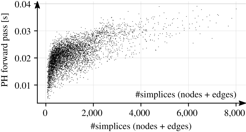
Figure 4: REDDIT-MULTI-5K timing experiments (in [s]) for persistent homology computation during one forward pass.

5.3 Results

Table 1 lists the results for the social networks. On both IMDB datasets, the Baseline performs en par with the state-of-the-art, as well as all readout strategies. However, this is not surprising as the graphs are very densely connected and substantial information is already encoded in the node degree. Consequently, using the degree as an initial node feature, combined with GNNs and various forms of readout does not lead to noticeable improvements.

REDDIT-* graphs, on the other hand, are far from fully connected and the global structure is more hierarchical. Here, the information captured by persistent homology is highly discriminative, with GFL outperforming SUM and SP (sort pooling) by a large margin. Notably, setting the filter function a-priori to the degree function performs equally well. We argue that this might already be an optimal choice on REDDIT. On other datasets (e.g., IMDB) this is not the case. Importantly, although the initial features on REDDIT graphs are set uninformative for all readout variants with 1-GIN, GFL can learn a filter function that is equally informative.

Method	PROTEINS	NCI1
Initial node features: $l(v)=\deg(v)$
PH-only	$73.5_{\pm 3.0}$	$67.8_{\pm 2.2}$
1-GIN (GFL)	$74.1_{\pm 3.4}$	$71.2_{\pm 2.1}$
1-GIN (SUM) (Xu et al., 2019)	$72.1_{\pm 3.5}$	$67.4_{\pm 3.0}$
1-GIN (SP) (Zhang et al., 2018a)	$72.4_{\pm 3.1}$	$67.8_{\pm 2.2}$
Baseline (Zaheer et al., 2017)	$73.1_{\pm 3.7}$	$65.8_{\pm 2.8}$
Initial node features $l(v)=[\deg(v),\operatorname{\textup{\text{lab}}}(v)]$
PH-only	n/a	n/a
1-GIN (GFL)	$73.4_{\pm 2.9}$	$77.2_{\pm 2.6}$
1-GIN (SUM) (Xu et al., 2019)	$75.1_{\pm 2.8}$	$77.4_{\pm 2.1}$
1-GIN (SP) (Zhang et al., 2018a)	$73.5_{\pm 3.8}$	$76.9_{\pm 2.3}$
Baseline (Zaheer et al., 2017)	$73.8_{\pm 4.4}$	$67.2_{\pm 2.3}$
State-of-the-Art (NN)
DCNN (Wang et al., 2018)	$61.3$	$62.6$
PatchySAN (Niepert et al., 2016)	$75.9$	$78.6$
DGCNN (Zhang et al., 2018a)	$75.5$	$74.4$
1-2-3-GNN (Morris et al., 2019)	$75.5$	$76.2$
5-GIN (SUM) (Xu et al., 2019)	$71.2$	$75.9$

Table 2: Graph classification accuracies (with std. dev.), averaged over ten cross-validation folds, on graphs with node attributes. Comparison to the state-of-the-art follows the results of Table 1.

Table 2 lists results on NCI1 and PROTEINS. On the latter, we observe that already the Baseline, agnostic to the connectivity information, is competitive to the state-of-the-art. GNNs with different readout strategies, including ours, only marginally improve performance. It is therefore challenging, to assess the utility of different readout variants on this dataset. On NCI1, the situation is different. Relying on node degrees only, our GFL readout clearly outperforms the other readout strategies. This indicates that GFL can successfully capture the underlying discriminative graph structure, relying only on minimal information gathered at node-level. Including label information leads to results competitive to the state-of-the-art without explicitly tuning the architecture. While all other readout strategies equally benefit from additional node attributes, the fact that 5-GIN (SUM) performs worse than 1-GIN (SUM) highlights our argument that message passing needs careful architectural design.

6 Discussion

To the best of our knowledge, we introduced the first approach to actively integrate persistent homology within the realm of GNNs, offering GFL as a novel type of readout. As demonstrated throughout all experiments, GFL, which is based on the idea of filtration learning, is able to achieve results competitive to the state-of-the-art on various datasets. Most notably, this is achieved with a single architecture that only relies on a simple one-level message passing scheme. This is different to previous works, where the amount of information that is iteratively aggregated via message passing can be crucial. We also highlight that GFL could be easily extended to incorporate edge level information, or be directly used on graphs with continuous node attributes.

As for the additional value of our readout operation, it leverages the global graph structure for aggregating the local node-based information. Theoretically, we established how to backpropagate a (gradient-based) learning signal through the persistent homology computation in combination with a differentiable vectorization scheme. For future work, it is interesting to study additional filtration techniques (e.g., based on edges, or cliques) and whether this is beneficial.

References

- Battaglia et al. (2016) Battaglia, P., Pascanu, R., Lai, M., Rezende, D., and Kavukcuoglu, K. Interaction networks for learning about objects, relations and physics. In NIPS, 2016.
- Bauer et al. (2014) Bauer, U., Kerber, M., and Reininghaus, J. Clear and compress: Computing persistent homology in chunks. In Topological Methods in Data Analysis and Visualization III, pp. 103–117. Springer, 2014.
- Bauer et al. (2017) Bauer, U., Kerber, M., Reininghaus, J., and Wagner, H. PHAT: Persistent homology algorithms toolbox. J. Symb. Comput., 78:76–90, 2017.
- Carrière et al. (2019) Carrière, M., Chazal, F., Ike, Y., Lacombe, T., Royer, M., and Umeda, Y. A general neural network architecture for persistence diagrams and graph classification. arXiv, 2019. https://arxiv.org/abs/1904.09378.
- Chen et al. (2019) Chen, C., Ni, X., Bai, Q., and Wang, Y. A topological regularizer for classifiers via persistent homology. In AISTATS, 2019.
- Duvenaud et al. (2015) Duvenaud, D., Maclaurin, D., Iparraguirre, J., Bombarell, R., Hirzel, T., Aspuru-Guzik, A., and Adams, R. Convolutional networks on graphs for learning molecular fingerprints. In NIPS, 2015.
- Edelsbrunner & Harer (2010) Edelsbrunner, H. and Harer, J. L. Computational Topology : An Introduction. American Mathematical Society, 2010.
- Edelsbrunner et al. (2002) Edelsbrunner, H., Letcher, D., and Zomorodian, A. Topological persistence and simplification. Discrete Comput. Geom., 28(4):511–533, 2002.
- Feragen et al. (2013) Feragen, A., Kasenburg, N., Petersen, J., Bruijne, M., and Borgwardt, K. Scalable kernels for graphs with continuous attributes. In NIPS, 2013.
- Gilmer et al. (2017) Gilmer, J., Schoenholz, S., Riley, P., Vinyals, O., and Dahl, G. Neural message passing for quantum chemistry. In ICML, 2017.
- Hamilton et al. (2017) Hamilton, W., Ying, R., and Leskovec, J. Inductive representation learning on large graphs. In NIPS, 2017.
- Hatcher (2002) Hatcher, A. Algebraic Topology. Cambridge University Press, Cambridge, 2002.
- Hofer et al. (2017) Hofer, C., Kwitt, R., Niethammer, M., and Uhl, A. Deep learning with topological signatures. In NIPS, 2017.
- Hofer et al. (2019a) Hofer, C., Kwitt, R., , Dixit, M., and Niethammer, M. Connectivity-optimized representation learning via persistent homology. In ICML, 2019a.
- Hofer et al. (2019b) Hofer, C., Kwitt, R., and Niethammer, M. Learning representations of persistence barcodes. JMLR, 20(126):1–45, 2019b.
- Kearns et al. (2016) Kearns, S., McCloskey, K., Berndl, M., Pande, V., and Riley, P. Molecular graph convolutions: Moving beyond fingerprints. Journal of Computer-Aided Molecular Design, 30(8):595–608, 2016.
- Kriege et al. (2016) Kriege, N., Giscard, P.-L., and Wilson, R. On valid optimal assignment kernels and applications to graph classification. In NIPS, 2016.
- Li et al. (2016) Li, Y., Tarlow, D., Brockschmidt, M., and Zemel, R. Gated graph sequence neural networks. In ICLR, 2016.
- Milosavljević et al. (2011) Milosavljević, N., Morozov, D., and Skraba, P. Zigzag persistent homology in matrix multiplication time. In SoCG, 2011.
- Morris et al. (2019) Morris, C., Ritzert, M., Fey, M., and Hamilton, W. Weisfeiler and Leman go neural: Higher-order graph neural networks. In AAAI, 2019.
- Niepert et al. (2016) Niepert, M., Ahmed, M., and Kutzkov, K. Learning convolutional neural networks for graphs. In ICML, 2016.
- Petri et al. (2013) Petri, G., Scolamiero, M., Donato, I., and Vaccarino, F. Networks and cycles: A persistent homology approach to complex networks. In ECCS, 2013.
- Rieck et al. (2019a) Rieck, B., Bock, C., and Borgwardt, K. A persistent Weisfeiler–Lehman procedure for graph classification. In ICML, 2019a.
- Rieck et al. (2019b) Rieck, B., Tognialli, M., Bock, C., Moor, M., Horn, M., Gumbsch, T., and Borgwardt, K. Neural persistence: A complexity measure for deep neural networks using algebraic topology. In ICLR, 2019b.
- Scarselli et al. (2009) Scarselli, F., Gori, M., Tsoi, A., hagenbuchner, M., and Monfardini, G. The graph neural network model. Transactions on Neural Networks, 20(1):61–80, 2009.
- Schütt et al. (2017) Schütt, K., Kindermans, P. J., Sauceda, H. E., Chmiela, S., Tkatchenko, A., and Müller., K. R. SchNet: A continuous-filter convolutional neural network for modeling quantum interactions. In NIPS, 2017.
- Shervashidze et al. (2009) Shervashidze, N., Vishwanathan, S., Petri, T., Mehlhorn, K., and Borgwardt, K. Efficient graphlet kernels for large graph comparison. In AISTATS, pp. 488–495, 2009.
- Shervashidze et al. (2011) Shervashidze, N., Schweitzer, P., van Leeuwen, E., Mehlhorn, K., and Borgwardt, K. Weisfeiler-lehmann graph kernels. JMLR, 12:2539–2561, 2011.
- Wang et al. (2018) Wang, Y., Sun, Y., Liu, Z., Sarma, S., Bronstein, M., and Solomon, J. Dynamic graph cnn for learning on point clouds. arXiv, 2018. https://arxiv.org/abs/1801.07829.
- Weisfeiler & Lehman (1968) Weisfeiler, B. and Lehman, A. A. A reduction of a graph to a canonical form and an algebra arising during this reduction. Nauchno-Technicheskaya Informatsia - Seriya 2, (9):12–16, 1968.
- Wu et al. (2020) Wu, Z., Pan, S., Chen, F., Long, G., Zhang, C., and Yu, P. A comprehensive survey on graph neural networks. IEEE Trans. Neural Netw. Learn. Syst, pp. 1–21, 2020.
- Xu et al. (2018) Xu, K., Li, C., Tian, Y., Sonobe, T., Kawarabayashi, K., and Jegelka, S. Representation learning on graphs with jumping knowledge networks. In ICML, 2018.
- Xu et al. (2019) Xu, K., Hu, W., Leskovec, J., and Jegelka, S. How powerful are graph neural networks? In ICLR, 2019.
- Ying et al. (2018) Ying, R., You, J., Morris, C., Ren, X., Hamilton, W., and Leskovec, J. Hierarchical graph representation learning with differentiable pooling. In NIPS, 2018.
- Zaheer et al. (2017) Zaheer, M., Kottur, S., Ravanbakhsh, S., Poczos, B., Salakhutdinov, R., and Smola, A. J. Deep sets. In NIPS, 2017.
- Zhang et al. (2018a) Zhang, M., Cui, Z., Neumann, M., and Chen, Y. An end-to-end deep learning architecture for graph classification. In AAAI, 2018a.
- Zhang et al. (2018b) Zhang, Z., Wang, M., Xiang, Y., Huang, Y., and Nehorai, A. Retgk: Graph kernels based on return probabilities of random walks. In NIPS, 2018b.
- Zhao & Wang (2019) Zhao, Q. and Wang, Y. Learning metrics for persistence-based summaries and applications for graph classification. In NeurIPS, 2019.