Soft phonons in the interface layer of the STO substrate can explain high temperature superconductivity in one unit cell $FeSe$.

Abstract

Using a microscopic model of lattice vibrations in the STO$\left(001\right)$ substrate, an additional $\Omega_{s}=50mev$ longitudinal optical (LO) interface mode is identified. The soft mode propagating mainly in the first $TiO_{2}$ layer (”$O$ chains”) has stronger electron - phonon coupling to electron gas in $FeSe$ than a well known $\Omega_{h}=100mev$ hard mode. The coupling constant, critical temperature, replica band are calculated. Although there exists a forward in the electron - phonon scattering peak, it is clearly not as sharp as assumed in recent theories (delta function - like). The critical temperature is obtained by solution of the gap equation and agrees with the observed one. The corresponding electron phonon coupling constant $\lambda=0.23$. The quasiparticle normal state ”satellite” in spectral weight is broad and its peak appears at frequency much higher than $\Omega_{s}$ consistent with observations usually associated with $\Omega_{h}$. Possible relation of the transversal counterpart of the surface LO soft mode with known phonons is discussed.

I Introduction.

The best known group of superconductors with critical temperature above $T_{c}=60K$, cuprates like $YBa_{2}Cu_{3}O_{7-\delta}$ ($93K$ at optimal doping) and $Bi_{2}Sr_{2}CaCu_{2}O_{8+x}$ ($92K$), are generally characterized by the following three structural/chemical peculiarities. First they are all quasi - 2D perovskite layered oxides. Second the 2D electron gas (2DEG) is created by maximally charging $CuO$ planes at optimal doping. Superconductivity resides in these layers. Third the layers (or by layers) are separated by several insulating ionic oxides. It is widely believedDagotto1 that, although the insulating layers play a role in charging the $CuO$ planes, the bosons responsible for the pairing are confined to the $CuO$ layer only.

Several years ago another group of high $T_{c}$ materials ($T_{c}=60-106K$) was fabricated by deposition of a single unit cell (1UC) layer of $FeSe$ on insulating substrates like $SrTiO_{3}$ (STO bothexpFeSe $\left(001\right)$ and110 $\left(110\right)$), $TiO_{2}$ (rutilerutileFeSe $\left(100\right)$ and anataseanataseFeSe $\left(001\right)$) andBa $BaTiO_{3}$. It is interesting to note that all three above features are manifest in this compounds as well. Indeed, the insulating substrates are again layered perovskite oxides. The electron gas residing in the $FeSe$ layercharging that is charged (doped) by the perovskite substrate. Of course there is a structural difference in that the the layered cuprates contain many $CuO$ planes, while there is a single $FeSe$ layer. The difference turns out not to be that important, since recently it was demonstratedXueBSCCO that even a single unit cell $CuO$ on top of $Bi_{2}Sr_{2}CaCu_{2}O_{8+x}$ film still retains high $T_{c}$. Moreover the pairing becomes of the nodeless s-wave variety as in the pnictides.

The role of the insulating substrate in the $FeSe$ systems however seems to extend beyond the charging charging . Although the physical nature of the pairing boson in cuprates is still under discussion (the prevailing hypothesis being that it ”unconventional”, namely not to be phonon - mediated), it became clear that superconductivity mechanism in $FeSe$ should at least include the substrate phonon exchange. There are several competing theories. One is an unconventional boson exchange within the pnictide plane (perhaps magnons Leerev , like that in other pnictides.’ superconductivity theoriesDagotto2 ). It intends to explain both the $40K\,$(upon optimal charging) superconductivity in $K$ or $Li$ intercalated $FeSe$intercalatedFeSe and ”boosting” of superconductivity by an interface $STO$ phonons above $60K$. Another point of viewour ; Gorkov ; DFT16 ; JohnsonNJP16 ; Kulic is that the ”intrinsic” pairing in the $FeSe$ plane is dominated by the pairing due to vibration of oxygen atoms in substrate oxide layers near the interface. Historically a smoking gun for the relevance of the phonon exchange to superconductivity has been the isotope effect. Very recentlyisotopeGuo the isotope ${}^{16}O$ was substituted, at least in surface layers of the $STO$(001) substrate, by ${}^{18}O$. For the same doping the gap at low temperature ($6K$) decreased by about 10%. Therefore the oxygen vibrations in the interface layers at least influence superconductivity.

Moreover detailed measurements of the phonon spectrum via high resolution electron energy loss spectroscopy (HREELS)Xue16phonon were performed. It demonstrated that the interface phonons are energetic (”hard” up to $\Omega_{h}=100mev$) for surface mode. This was corroborated by the DFT calculationsDFT16 . The phonons couple effectively to the electron gas, as became evident from clear identification by ARPES of the replica bandLee12 ; Johnson16 . The explanation of the replica bands was based on the forward peak in the electron - phonon scattering. Initially this inspired an idea that the surface phonons alone could provide a sufficiently strong pairingJohnsonNJP16 ; Kulic . The values of the coupling constant deduced from the intensity of the replica bands however was found to be rather small $\lambda<0.25$. The BCS scenario, $T_{c}\approx\Omega_{h}e^{-1/\lambda}$, is clearly out, even when possible violation of the Migdal theorem due to nonadiabaticity ($\Omega_{h}>E_{F}$) is accounted forour . One therefore had to look for other ideas. One is provided by a possibility of the extreme, delta like, scattering peak modelKulicrev , for which $T_{c}\approx\frac{\lambda}{2+3\lambda}\Omega_{h}$. Indeed one can obtainJohnsonNJP16 ; Kulic high $T_{c}$ even for such a small $\lambda$, but only for rather restrictive values of parameters of the ionic substrate model (within the macroscopic dipole approximation electrodynamics). Recently attempts were made to solve the Eliashberg equation for the phonon mediated couplingAperis derived directly in the framework of the density functional (DFT) approachDFTnew .

In the present paper we consider a sufficiently precise microscopic model of phonons in the ionic STO$\left(001\right)$ substrate (beyond the phenomenological dipole approximation approach) and find an additional much softer LO interface mode that is as strongly coupled to the electron gas in the $FeSe$ layer as the hard mode. The only parameters entering the model are the Born-Meyer inter - atomic potentialsAbrahamson and measured atomic chargesaverestov . The coupling $\lambda$, critical temperature, replica band and other characteristics of the superconducting state are calculated and are consistent with experimental observations. Although there exists a forward in the electron - phonon scattering peak, it is clearly not a delta - like. The gap equations for the phonon - mediated pairing are solved without this assumption. The soft mode $\Omega_{s}$ propagating mainly in the first $TiO_{2}$ layer (”$O$ chains”) contribute much more than the highest frequency $\Omega_{h}$ mode to the pairing.

II The interface structure, symmetry.

II.1 Structure of several top layers.

The structure of the best studied high $T_{c}$ monolayer $FeSe$ system, that on the STO substrate oriented along the $\left(001\right)$ is as follows The top three layers, where 2D electron gas resides, are $Se,Fe,Se$, while the first substrate layer is $TiO_{2}$. The next layer is - $SrO$

Let us summarize experimentally determined configurations of atoms in the one unit cell $FeSe/STO$ in a form sufficiently accurate for the phonon spectrum calculation. The top three layers, $Se$ (1 and 3, green rings) and $Fe$ (brown ring), where 2D electron gas resides, are shown on the left of Fig.SM1. The first substrate layer is $TiO_{2}$, as determined by STS is shown in the center ($Ti$ - blue rings, $O$ - red full circle), while the next layer is - $SrO$ (on the right, $Sr$ - cyan rings, $O$ - dark red full circle). Below this plane the STO pattern is replicated. Out of plane spacings counted from the $TiO_{2}$ layer are specified in Table I.

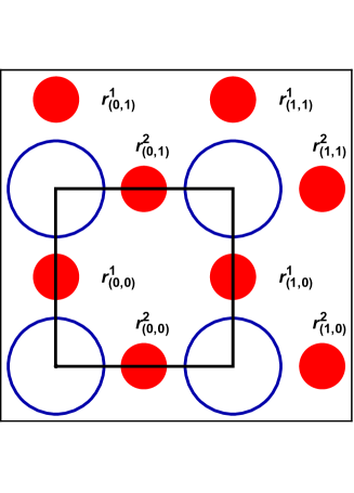
Figure 1: The top $TiO_{2}$ substrate layer. Blue empty circles represent the $Ti$ atoms, while red filled ones represent light $O$ atoms. Unit cell is depicted as a black square. Locations of the two sublattices in Eq.(2) are shown.

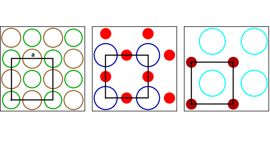
Figure 2: Structure of the surface layers. On the left $Fe$ (brown) and $Se$ (green) planes are projected. In the center the $TiO_{2}$ ($Ti$ - blue , $O$ - red), while on the right s the adjuscent $SrO$ ($St$ cyan, , $O$ - dark red).

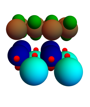
Figure 3: 3D view of the surface layers composing one unit cell :molecule”. Colors as in Fig.SM1. Sizes of atoms are inversely to the values of the Born - Mayer parameter $b$.

Fig.3 is a 3D view of the molecule with sphere radii corresponding to the repulsive Meyer potential ranges given in Table I.

Table 1: Atomic parameters.

atom	$O$ in $TiO_{2}$	$Ti$	$Sr$	$Se$	$O$ in $SrO$
mass (a.u.)	$16$	$48$	$88$	$79$	$16$
$A\,\ \text{(}kev\text{)}$	$2.143$	$9.353$	$20.785$	$17.56$	$2.143$
$b$  ($A^{-1}$)	$3.388$	$3.598$	$3.541$	$3.511$	$3.388$
charge $Z$	$-1.27$	$2.54$	$1.85$	$0$	$-1.36$
spacing $z$ ($A\,$)	$0$	$0$	$-1.6$	$3.7$	$-1.6$

II.2 The unit cell and symmetry of the whole system

The square translational symmetry in the lateral ($x,y$) directions of the system has two basis vectors shown in Fig.1, Unit cell including both the metallic layer and the substrate containing $Fe_{2}Se_{2}TiSrO_{3}$ is marked by the black frame in Fig. 4. The lattice spacing, that coincides with the distance between the $Ti$ atoms is $a=3.9A$, equal to the distance between the $Se$ atomsXueSTS . The square translational symmetry in the lateral ($x,y$) directions of the system has two basis vectors shown in Fig.1. The lattice spacing, that coincides with the distance between the $Ti$ atoms is $a=3.9A$, equal to the distance between the $Se$ atomsXueSTS .

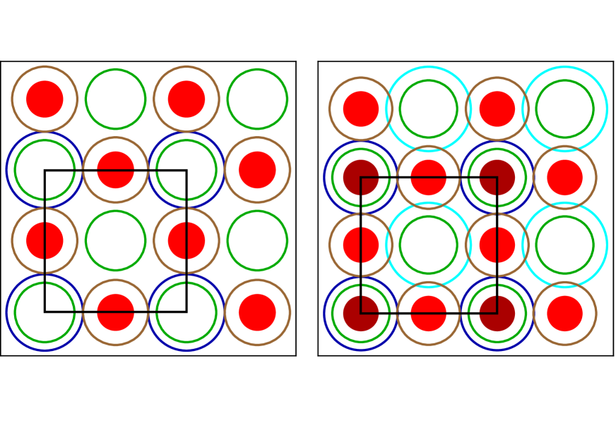
Figure 4: Left. $FeSe$ with the first $TiO_{2}$ layer. Colors are same as in Fig. SM1.

The left panel of Fig. 4 contains the projection of $FeSe$ and $TiO_{2}$, while the whole ”molecule” including the $SrO$ layer is given on the right panel.

III Model the 2D electron gas in FeSe interacting with phonons in the STO substrate.

III.1 Electron gas.

Our model consists of the 2DEG interacting with surface phonons of polar insulator $STO$:

$$H=H_{e}+H_{ph}+H_{e-ph}\text{.}$$ (1)

The Fermi surface consists of two slightly distinct electron pockets centered around the crystallographic $M$ - point. Although experimentisotopeGuo shows four - fold symmetry breaking, it is much smaller than the asymmetry of the superconducting order parameter and will be neglected. The electron gas is described sufficiently well by a simple tight binding model on square lattice with spacing $a=3.9A$, proposed in ref DFT13 . Electrons are hoping between the $Fe$ $4d_{xz}$ and $4d_{yz}$ orbitals around locations of $Fe$ atoms on two sublattices, $A=1,2$, see Fig.1:

$$\mathbf{r}_{\mathbf{m}}^{1}=a\left(m_{1},\frac{1}{2}+m_{2}\right);\text{ \ }\mathbf{r}_{\mathbf{m}}^{2}=a\left(\frac{1}{2}+m_{1},m_{2}\right)\text{.}$$ (2)

Hopping occurs on each sublattice independently with amplitude $t$. The overlap between nearest neighbors is negligible due to symmetry of orbitals. In momentum representation on the 2D Brillouin zone (BZ), $-\pi/a<k_{x},k_{y}<\pi/a$, one has (neglecting the spin $\sigma$ dependenceDFT13 ):

$$H_{e}=\sum\nolimits_{\mathbf{k}}c_{\mathbf{k}}^{A\sigma\dagger}\left(\epsilon_{\mathbf{k}}-\epsilon_{F}\right)c_{\mathbf{k}}^{A\sigma}\text{,}$$ (3)

where $\epsilon_{\mathbf{k}}=-2t\left(2+\cos\left[ak_{x}\right]+\cos\left[ak_{y}\right]\right)$. It is sufficient for our purposes to use a parabolic approximation with an effective mass $m^{\ast}=2.7m_{e}$ and Fermi energyLee14 $\epsilon_{F}=60meV$. The electron gas is considered non - interacting although screened delta - like repulsive interaction should be added to the gap equation as discussed inour .

III.2 Optical phonon modes in the $TiO_{2}$ layer.

Phonons in ionic crystals are described by the Born - Meyer potential due to electron’s shells repulsionAbrahamson and electrostatic interaction of ionic charge,

$$V^{XY}\left(r\right)=\sqrt{A_{X}A_{Y}}\exp\left[\frac{1}{2}\left(b^{X}+b^{Y}\right)r\right]+Z_{X}Z_{Y}\frac{e^{2}}{r}\text{,}$$ (4)

with values of coefficients $A$ and $b$ listed in Table I. The ionic charges of the STO plane below the last $TiO_{2}$ are taken from a DFT calculation averestov of the Millikan charges (performed without $FeSe$). In the $TiO_{2}$ layer the charges are determined by neutrality, and a requirement that the position of the oxygen atoms between the two $Ti$ atoms is a minimum of potential.

It is reasonable to expect that the modes most relevant for the electron - phonon coupling across the interface are the vibrations of the atoms in the $TiO_{2}$ layer, see Fig.5. Since oxygen is much lighter than $Ti$, we assume that $Ti$ atoms’ vibrations are negligible. Obviously we lose acoustic branch, however the acoustic phonons are not expected to contribute to pairingMahan ; Gorkov . Atoms in neighboring layers can also be treated as static. Moreover one can neglect more distant layers both in STO (beyond $SrO$) and in $FeSe$. Even the influence of the lower $Se$ layer is insignificant due to the distance. Therefore the dominant lateral displacements, $u_{\mathbf{m}}^{A\alpha}$, $\alpha=x,y$, are of the two oxygen sublattices directly beneath the corresponding $Fe$ sites of Eq.(2). The dynamic matrix $\left[D_{\mathbf{q}}\right]_{\alpha\beta}^{AB}$ is calculated by expansion of energy to second order in oxygen displacement (details in Appendix I), so that Hamiltonian is:

$$H_{ph}=\frac{1}{2}\sum\nolimits_{\mathbf{q}}\left\{M\frac{du_{-\mathbf{q}}^{\alpha A}}{dt}\frac{du_{\mathbf{q}}^{\alpha A}}{dt}+u_{\mathbf{-q}}^{\alpha A}\left[D_{\mathbf{q}}\right]_{\alpha\beta}^{AB}u_{\mathbf{q}}^{\beta B}\right\}\text{.}$$ (5)

Here $M$ is the oxygen mass. Summations over repeated sublattice and components indices is implied. Now we turn to derivation of the phonon spectrum and the electron - phonon coupling.

IV Phonon spectrum and the electron - phonon interactions

IV.1 Phonon spectrum

Four eigenvalues are given in Fig. 6, while their polarization for a small $\mathbf{q}$ vector in $\mathbf{x}$ direction depicted in Fig. 5. One observes that there are high and low frequency modes are in the range $\Omega_{\mathbf{q}}^{h}\sim 100-120mev$ and $\Omega_{\mathbf{q}}^{s}\sim$ $20-50mev$ respectively. The energy of LO modes (blue in Fig. 6) is larger than that of the corresponding TO (red), although the sum $\Omega_{\mathbf{q}}^{LO}+\Omega_{\mathbf{q}}^{TO}$ is nearly dispersionless. At $\Gamma$ the splitting is small, while due to the long range Coulomb interaction there is hardening of LO and softening of TO at the BZ edges. The dispersion of the high frequency modes is small, while for the lower frequency mode it is more pronounced.

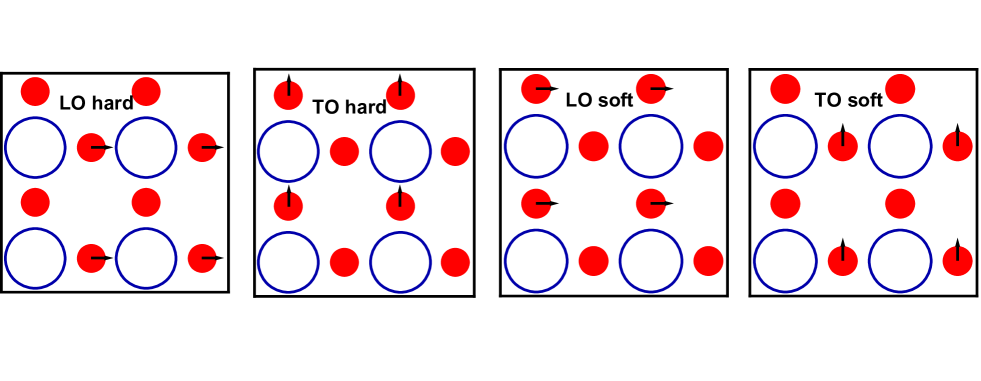
Figure 5: Oxygen atoms vibrations in the $TiO_{2}$ plane. Polarization of the phonons with momentum along the $x$ axis. The oxygen atoms displacement;s directions are indicated by arrows. Sublattice A=1 (see Eq.(2)) is active in the hard TO and solf LO

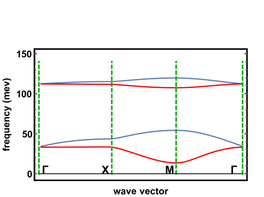
Figure 6: Spectrum of phonons in the $TiO_{2}$ plane. Blue lines correspond to tranverse, while red line to the transverse modes.

Geometrically it is clear that the low frequency $\Omega_{\mathbf{q}}^{s}$ arises due the ”empty site” at point $\left(1/2,1/2\right)a$, Fig.1. Physically the softness of the TO mode means that the crystal is close to the ferroelectric transition of the displacement type characteristic to oxides in perovskitesferroelectric (the lowest frequency at the $M$ point of soft TO mode, $\Omega_{\mathbf{q=M}}^{sTO}$ would have reached zero if the transition have occurred). Although the soft LO mode, $\Omega_{\mathbf{q}}^{sLO}$ (important for the electron - phonon coupling) is slightly higher than $\Omega_{\mathbf{q}}^{sTO}$, it is still lower than $\Omega_{\mathbf{q}}^{h}$   by a significant factor $2.5$.

IV.2 Electron - phonon coupling

The STO surface phonons interaction with the 2DEG on the $Fe$ layer $z_{Fe}=4.4A$ above the $TiO_{2}$ plane is determined by the electric potential created near the $4d$ $Fe$ orbitals:

$$\Phi\left(r\right)=-Z_{O}e\sum\limits_{\mathbf{m,}A}\frac{\left(\mathbf{r}-\mathbf{r}_{\mathbf{m}}^{A}\right)\cdot\mathbf{u}_{\mathbf{m}}^{A}}{\left(\left(\mathbf{r}-\mathbf{r}_{\mathbf{m}}^{A}\right)^{2}+z_{Fe}^{2}\right)^{3/2}}\text{.}$$ (6)

It is important that the by vibrating charged oxygen atoms in the last $TiO_{2}$ layer reside directly below $Fe$ atoms. Influence on the electron - phonon coupling of vibrating $Ti$ atoms of the first layer is further reduced since they are not situated directly beneath the $Fe$ sites.

The potential generated by the charged $TiO_{2}$ oxygen vibration mode $u_{\mathbf{m}}^{A}$ at arbitrary point $\mathbf{r}$ is (namely ignoring contributions from other charged ions is,

$$\Phi\left(\mathbf{r},z\right)=\sum\nolimits_{\mathbf{m,}A}\frac{Z_{O}\text{ }e}{\sqrt{\left(\mathbf{r}-\mathbf{r}_{m}^{A}-\mathbf{u}_{\mathbf{m}}^{A}\right)^{2}+z^{2}}}\text{,}$$ (7)

where the distance is to the $Fe$ layer, $z=z_{Fe}=4.4A.$ Expanding in displacement, one  obtains:

$$\Phi\left(\mathbf{r},z\right)\approx\Phi_{e-i}^{0}\left(\mathbf{r},z\right)-Z_{O}\text{ }e\sum\nolimits_{\mathbf{m,}A}\frac{\left(\mathbf{r}-\mathbf{r}_{\mathbf{m}}^{A}\right)\cdot\mathbf{u}_{\mathbf{m}}^{A}}{\left(\left|\mathbf{r}-\mathbf{r}_{\mathbf{m}}^{A}\right|^{2}+z^{2}\right)^{3/2}}\text{.}$$ (8)

The Hamiltonian for interaction with electrons on the $4d$ $Fe$ orbitals with wave functions $\varphi_{\mathbf{l}}^{A}\left(\mathbf{r},z\right)$ (on both sublattices $A=1,2$), $H_{ei}=\int_{\mathbf{r}}\Phi\left(\mathbf{r}\right)\widehat{n}_{\mathbf{r}}$, expanded to first order in the oxygen vibrations consequently is,

$$H_{ei}=-Z_{O}e^{2}\int_{\mathbf{r},z}\sum\nolimits_{\mathbf{m,}A,B}\frac{\left(\mathbf{r}-\mathbf{r}_{\mathbf{m}}^{A}\right)\cdot\mathbf{u}_{\mathbf{m}}^{A}}{\left(\left(\mathbf{r}-\mathbf{r}_{\mathbf{m}}^{A}\right)^{2}+z^{2}\right)^{3/2}}\left|\varphi_{\mathbf{l}}^{A}\left(\mathbf{r},z\right)\right|^{2}\widehat{c}_{\mathbf{l}}^{\sigma B\dagger}\widehat{c}_{\mathbf{l}}^{\sigma B}\text{.}$$ (9)

Sublattice indices are $A=1,2$ for oxygen and $B=1,2$ for $Fe$. Although the most general matrix element depends also on the electron momentum $\mathbf{k}$ in addition to the phonon momentum $\mathbf{q}$, it does not appear in Eq.9 since the coupling is to the density, namely the size of the $Fe$ orbital is neglected. Indeed the localized (the tight binding) form, namely, neglecting the size of the orbital, $\left|\varphi_{\mathbf{l}}^{A}\left(\mathbf{r},z\right)\right|^{2}=\delta\left(\mathbf{r-r}_{\mathbf{l}}^{B}\right)\delta\left(z-z_{Fe}\right)$, where $z_{Fe}$ is given in Table I, reads:

$$H_{ei}=-Z_{O}e^{2}\int_{\mathbf{r},z}\sum\nolimits_{\mathbf{l},\mathbf{m,}A,B}\frac{\left(\mathbf{r}_{\mathbf{l}}^{B}-\mathbf{r}_{\mathbf{m}}^{A}\right)\cdot\mathbf{u}_{\mathbf{m}}^{A}}{\left(\left(\mathbf{r}-\mathbf{r}_{\mathbf{m}}^{A}\right)^{2}+z_{Fe}^{2}\right)^{3/2}}\widehat{n}_{\mathbf{l}}^{B\dagger}\text{.}$$ (10)

Here the density operator $\widehat{n}_{\mathbf{l}}^{B\dagger}=\widehat{c}_{\mathbf{l}}^{\sigma B\dagger}\widehat{c}_{\mathbf{l}}^{\sigma B}$. The interaction electron-phonon Hamiltonian has the form

$$H_{ei}=-e\int_{\mathbf{r}}\Phi\left(\mathbf{r}\right)\widehat{n}_{\mathbf{r}}=Z_{O}e^{2}\sum\nolimits_{\mathbf{q}}\widehat{n}_{-\mathbf{q}}^{B}g_{\mathbf{q}}^{BA\alpha}\widehat{u}_{\mathbf{q}}^{A\alpha}\text{,}$$ (11)

with $\widehat{n}_{\mathbf{q}}^{B}$ being Fourier transform of the electron density operator on sublattice $B$ of $Fe$ and

$$\mathbf{g}_{\mathbf{q}}^{BA}=\sum\nolimits_{\mathbf{m}}e^{ia\mathbf{q\cdot m}}\frac{\mathbf{r}_{\mathbf{m}}^{A}-\mathbf{r}_{\mathbf{0}}^{B}}{\left(\left|\mathbf{r}_{\mathbf{m}}^{A}-\mathbf{r}_{\mathbf{0}}^{B}\right|^{2}+z_{Fe}^{2}\right)^{3/2}}\text{,}$$ (12)

Grimvall ; Eliashberg . The later depends on sublattices of both the vibrating oxygen atoms $A$ and the $Fe$ orbital hosting the electron on sublattice $B$ (in addition to the polarization $\alpha$). It is well known that only longitudinal phonons contribute to the effective electron - electron interaction, as is clear from the scalar product form of the Eq.(11). To conclude Eqs.(3,5,11) define our microscopic model. In order to describe superconductivity, one should ”integrate out” the phonon degrees of freedom to calculate the effective electron - electron interaction. The discrete Fourier transform,

$$\widehat{n}_{\mathbf{l}}^{B}=\frac{1}{N_{s}}\sum\nolimits_{\mathbf{q}}\exp\left[-\frac{2\pi i}{N_{s}}\mathbf{q}\cdot l\right]\widehat{n}_{\mathbf{q}}^{B},$$ (13)

together with Eq.(11), result in the Matsubara action

$$\mathcal{A}_{eph}\left[\psi,u\right] = \frac{Z_{O}e^{2}}{T}\sum\nolimits_{\mathbf{q,}n}n_{-\mathbf{q},-n}^{B}\left[\psi\right]g_{\mathbf{q}}^{\alpha BA}u_{\mathbf{q},n}^{\alpha A}\text{;}$$ (14)

$$n_{-\mathbf{q},-n}^{B}\left[\psi\right] = \sum\nolimits_{\mathbf{k,}m}\psi_{\mathbf{k}-\mathbf{q},m-n}^{\ast\sigma B}\psi_{\mathbf{k},m}^{\sigma B}\text{.}$$

that will be used below.

The electron - phonon coupling functions defined by,

$$\rho_{\mathbf{q}}^{iA}\equiv\sum\nolimits_{C}\mathbf{e}_{\mathbf{q}}^{iC}\cdot\mathbf{g}_{\mathbf{q}}^{CA}\text{,}$$ (15)

depends on two indices, the phonon mode $i$ and a sublattice index $A$. The ”geometric” function $\mathbf{g}_{\mathbf{q}}^{CA}$ is defined in Eq.(8) of the main text.

Figure 7: Electron - phonon coupling dependence on quasimomentum $\mathbf{q}$ (matrix element) on a quarter of Brillouin zone. The forward scattering peak is clearly manifest.

Figure 8: Fit of the electron - phonon nteraction strangth of the soft mode by an exponential function of Eq. 18of the main text.

The corresponding plots for sublattice $A=2$ are rotated by $\pi/2$ due to the fourfold symmetry. The continuos rotation symmetry is weakly broken at edges of the Brillouin zone. The shape is slightly different for the hard and soft mode, however the rotation invariant fit of Eq.(16) is correct to $5\%$ as seen in Fig. 7. The transversal modes are smaller by an order of magnitude.

The mostly transversal contributions $\rho_{\mathbf{q,}h}^{A}$ and $\rho_{\mathbf{q,}s}^{A}$ are negligible (albeit nonzero for general $\mathbf{q}$ due to lack of continuous rotational symmetry). The LO contributions can be approximated within 1% (see Fig.8) by

$$\rho_{\mathbf{q}}^{A}\approx\rho e^{-\left|\mathbf{q}\right|/q_{0}}\text{,}$$ (16)

with $\rho=2\pi/a^{2}\$and $q_{0}=1/z_{Fe}=0.9/a\approx 0.23A^{-1}$ for both modes. The exponential decrease reflectsLee12 ; JohnsonNJP16 ; Kulic the distance between the phonon layer and the 2DEG.

IV.3 Effective electron - electron interaction.

To take into account finite temperature, we employ the Matsubara actionour for the above Hamiltonian, $\mathcal{A}=\mathcal{A}_{e}+\mathcal{A}_{ph}+\mathcal{A}_{eph}$, where

$$\mathcal{A}_{e} = T^{-1}\sum\nolimits_{\mathbf{k},n}\psi_{\mathbf{k},n}^{\ast\sigma A}\left(G_{\mathbf{k},n}^{0}\right)^{-1}\psi_{\mathbf{k},n}^{\sigma A}\text{, }\mathcal{A}_{ph}=\frac{M}{2T}\sum\nolimits_{\mathbf{q,}n}u_{-\mathbf{q},-n}^{\alpha A}\left[\Pi_{\mathbf{q},n}\right]_{\alpha\beta}^{AB}u_{\mathbf{q,}n}^{\beta B};$$ (17)

$$\text{ }\mathcal{A}_{eph} = \frac{Z_{O}e^{2}}{T}\sum\nolimits_{\mathbf{q,}n}n_{-\mathbf{q},-n}^{B}g_{\mathbf{q}}^{\alpha BA}u_{\mathbf{q},n}^{\alpha A}\text{.}$$

Here the bare Green’s function for normal electrons described by a Grassmanian field $\psi$, is,

$$G_{\mathbf{k},n}^{0}=\left(i\omega_{n}^{f}-\epsilon_{\mathbf{k}}+\epsilon_{F}\right)^{-1}\text{,}$$ (18)

with $\omega_{n}^{f}=\pi T\left(2n+1\right)$. Here the density is written in terms of. The $4\times 4$ polarization matrix,

$$\left[\Pi_{\mathbf{q},n}\right]_{\alpha\beta}^{AB}=\left(\omega_{n}^{b}\right)^{2}\delta^{AB}\delta_{\alpha\beta}+M^{-1}\left[D_{\mathbf{q}}\right]_{\alpha\beta}^{AB}\text{,}$$ (19)

is defined via the dynamic matrix of Eq.(5) calculated in Appendix I and $\omega_{n}^{b}=2\pi nT$ is the Matsubara frequency for phonons. The action is completed by the free electron action,

Since the action is quadratic in the phonon field $\mathbf{u}$ the partition function is gaussian, it can be integrated out exactly. The electronic effective action is obtained by integration of the partition function over the phonon field,

$$e^{-\mathcal{A}_{eff}\left[\psi\right]}=\int_{u}e^{-\mathcal{A}_{ph}\left[u\right]-\mathcal{A}_{eph}\left[\psi,u\right]}\text{,}$$ (20)

where the phonon action is

$$\mathcal{A}_{ph}=\frac{M}{2T}\sum\nolimits_{\mathbf{q,}n}u_{-\mathbf{q},-n}^{\alpha A}\left[\Pi_{\mathbf{q},n}\right]_{\alpha\beta}^{AB}u_{\mathbf{q,}n}^{\beta B}\text{,}$$ (21)

and the electron - phonon part is given by Eq.(10) .

The integral is gaussian in the fields $u_{\mathbf{q}n}^{\beta B}$ and thus, since normalization constant is independent of the electron field in $n_{-\mathbf{q}n}^{B}$, is performed by completion to full square. The result collecting the constants is,

$$e^{-\mathcal{A}_{eff}\left[\psi\right]}\propto\exp\left[-\frac{\left(Z^{O}e^{2}\right)^{2}}{2MT}\sum\nolimits_{\mathbf{q,}n}n_{\mathbf{q},n}^{B}g_{\mathbf{q}}^{BC\gamma}\left[\Pi_{\mathbf{q},n}^{-1}\right]_{\gamma\delta}^{CD}g_{-\mathbf{q}}^{DA\delta}n_{-\mathbf{q},-n}^{A}\right]\text{.}$$ (22)

As a result one obtains the effective density - density interaction term for of electrons

$$\mathcal{A}_{eff}=\frac{1}{2T}\sum\nolimits_{\mathbf{q}.n}n_{\mathbf{q},n}^{B}v_{\mathbf{q},n}^{BA}n_{-\mathbf{q},-n}^{A}\text{,}$$ (23)

where the effective electron - electron frequency dependent potential is

$$v_{\mathbf{q},n}^{BA}=-\frac{\left(Z_{O}e^{2}\right)^{2}}{M}g_{\mathbf{q}}^{BC\gamma}\left[\Pi_{\mathbf{q},n}^{-1}\right]_{\gamma\delta}^{CD}g_{-\mathbf{q}}^{DA\delta}\text{.}$$ (24)

In the basis of the four phonon modes with polarization vectors $\mathbf{e}_{\mathbf{q}}^{iC}$ depending on the phonon branch $i=1,...4$, this becomes:

$$v_{\mathbf{q},n}^{BA}=-\frac{\left(Z_{O}e^{2}\right)^{2}}{M}\sum\nolimits_{i=1}^{4}\frac{\rho_{\mathbf{q,}i}^{B}\rho_{-\mathbf{q,}i}^{A}}{\omega_{n}^{b2}+\Omega_{\mathbf{q,}i}^{2}}\text{; \ }\rho_{\mathbf{q,}i}^{A}\equiv\sum\nolimits_{C}\mathbf{e}_{\mathbf{q}}^{iC}\cdot\mathbf{g}_{\mathbf{q}}^{CA}\text{.}$$ (25)

Consequently Eq.(25) takes a form:

$$v_{\mathbf{q},n}^{AB}\approx-\frac{\left(Z_{O}e^{2}\rho\right)^{2}}{M}e^{-2\left|\mathbf{q}\right|/q_{0}}\left(\frac{1}{\omega_{n}^{b2}+\Omega_{\mathbf{q,}h}^{2}}+\frac{1}{\omega_{n}^{b2}+\Omega_{\mathbf{q,}s}^{2}}\right)\text{,}$$ (26)

approximately independent of sublattice indices. One observes that at $nT<<\Omega$ the dominant mode one is the soft LO mode for superconductivity and even for satellites.

V Superconductivity. 

V.1 Gap equation

The STM experimentsswave demonstrate that the order parameter is gapped (hence no nodes) and indicate a weakly anisotropic spin singlet pairing. Therefore we look for solutions for the normal and the anomalous Green’s function of the Gorkov equations in the form

$$\left\langle\psi_{\mathbf{k},n}^{\rho B}\psi_{\mathbf{k},n}^{\ast\sigma A}\right\rangle=\delta^{\sigma\rho}G_{\mathbf{k},n}^{AB};\text{ }\left\langle\psi_{\mathbf{k},n}^{\sigma A}\psi_{-\mathbf{k},-n}^{\rho B}\right\rangle=\varepsilon^{\sigma\rho}F_{\mathbf{k},n}^{AB}$$ (27)

where $\varepsilon^{\sigma\rho}$ is the antisymmetric tensor. At criticality, $G_{\mathbf{k},n}^{AC}=\delta^{AC}G_{\mathbf{k},n}^{0}$ (normal Green’s function not renormalized significantly at weak coupling), the Gorkov equation for the anomalous Greens function is (derived for a multi - band system in Appendix B):

$$F_{\mathbf{p},m}^{AC}+T_{c}\left|G_{\mathbf{p},m}^{0}\right|^{2}\sum\nolimits_{\mathbf{q},n}v_{\mathbf{p-q},m-n}^{AC}F_{\mathbf{q},n}^{AC}=0\text{.}$$ (28)

In terms of the gap function,

$$\Delta_{\mathbf{p},m}^{AC}=T_{c}\sum\nolimits_{\mathbf{k},n}v_{\mathbf{p-k},m-n}^{AC}F_{\mathbf{k},n}^{AC}\text{,}$$ (29)

this becomes

$$T_{c}\sum\nolimits_{\mathbf{p},m}\left|g_{\mathbf{p},m}^{0}\right|^{2}v_{\mathbf{q-p},n-m}^{AC}\Delta_{\mathbf{p},m}^{AC}=-T_{c}\sum\nolimits_{\mathbf{p},m}\frac{v_{\mathbf{q-p},n-m}^{AC}}{\left(\omega_{m}^{e}\right)^{2}+\left(\epsilon_{\left|\mathbf{p}\right|}-\epsilon_{F}\right)^{2}}\Delta_{\mathbf{p,}m}^{AC}=\Delta_{\mathbf{q},n}^{AC}\text{.}$$ (30)

From this point on let us assume that we consider just the dominant mode and that this mode is dispersionless., see Eq.(26) $\Omega_{\mathbf{q}s}=\Omega_{s}$. In addition only element $v_{\mathbf{q},n}^{11}=v_{\mathbf{q},n}^{22}$ is considered, so that the sublattice index will be omitted. The resulting sum near a circular Fermi surface can be approximated by an integral:

$$\frac{T_{c}\left(Z_{O}e^{2}\rho\right)^{2}}{M}\sum\nolimits_{m}\frac{1}{\omega_{n-m}^{b2}+\Omega^{2}}\frac{1}{\left(2\pi\right)^{2}}\int_{\mathbf{p}}\frac{e^{-2\left|\mathbf{q-p}\right|/q_{0}}}{\left(\omega_{m}^{e}\right)^{2}+\left(\epsilon_{\left|\mathbf{p}\right|}-\epsilon_{F}\right)^{2}}\Delta_{\mathbf{p,}m}=\Delta_{\mathbf{q,}n}\text{.}$$ (31)

Using rotation invariance one obtains the following gap equation for an angle independent gap function, $\Delta_{\mathbf{p,}m}=\Delta_{p\mathbf{,}m}$, in polar coordinates:

$$\frac{T_{c}\left(Z_{O}e^{2}\rho\right)^{2}}{M\left(2\pi\right)^{2}}\sum\nolimits_{m}\frac{1}{\omega_{n-m}^{b2}+\Omega^{2}}\int_{p=0}\frac{p\text{ \ }\gamma\left[p,q\right]}{\left(\omega_{m}^{e}\right)^{2}+\left(\epsilon_{p}-\epsilon_{F}\right)^{2}}\Delta_{p\mathbf{,}m}=\Delta_{q\mathbf{,}n}\text{.}$$ (32)

The integration over the difference of angles can be performed numerically,

$$\gamma\left[p,q\right]=\int_{\phi=0}^{2\pi}\exp\left[-2\sqrt{p^{2}+q^{2}-2pq\cos\phi}/q_{0}\right]\text{.}$$ (33)

This eigenvalue problem was first solved numerically and then (in Appendix C) within the Eliashberg approximation in the case when the main contribution comes from momenta very close to $k_{F}$. Both methods gives the same value for the critical temperature $T_{c}=51K$

V.2 Solution of the gap equation

Momenta within the circular Brillouin zone of radius $\pi/a$ were discretized as $p\rightarrow\frac{\pi}{N_{s}a}p$ with $N_{s}=400$, while the Matsubara frequency $m$ was truncated at $\left|\pi T_{c}\left(2m-1\right)\right|\simeq 4\Omega_{s}$. Time reversal symmetry ensures $\Delta_{p,-m}=\Delta_{p,m+1}$, so that only positive integers were included

$$K_{pm,qn}\Delta_{p\mathbf{,}m} = \Delta_{q\mathbf{,}n}$$ (34)

$$K_{pm,qn} = \frac{T_{c}\left(Z_{O}e^{2}\rho\right)^{2}}{MN_{s}}\frac{p\text{ \ }\gamma\left[p,q\right]}{\left(\omega_{m}^{e}\right)^{2}+\left(\epsilon_{p}-\epsilon_{F}\right)^{2}}$$

The critical temperature is obtained when the largest eigenvalue of the matrix $K$ Eq.( 32) is unit. The numerical results are the following. $T_{c}=51K$, while for isotope ${}^{18}O$ it becomes $T_{c}=49K$.

It is clearly demonstrated in Fig. 9 that the dependence on $m$ is very strong: the two lowest Matsubara frequencies $\Delta_{m}$, $m=0,1$ for which $\left|\pi T\left(2m-1\right)\right|=\pi T$ are dominant, while corrections of $m=-3,4$ (yellow line in Fig. 9) become less than 1%.

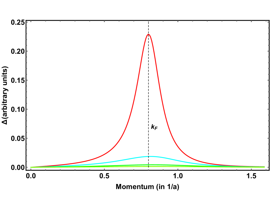
Figure 9: Gap function for different Matsubara frequences The m=0,1 (red) is dominant, while strength of the subleading correlators, m=-1,2 (cyan), m=-2,3 (green), m=-3,4 (yellow), decrease fast.

Shape of the momenta distribution of all the modes can be described as a Lorenzian around $k_{F}$. The width is significant due to exceptionally small ”adiabaticity parameter” $E_{F}/\Omega_{s}=1.4$ (would be smaller for the hard mode $\Omega_{h}$). The Lorenzian width shrinks to zero for small $q_{0}$ (the delta forward peak scattering limit) and for adiabatic case of large $E_{F}/\Omega_{s}$. The gap function $\Delta_{k,\omega}$ vanishes at the transition temperature and increases below it as $\left(T-T_{c}\right)^{1/2}$ according to Ginzburg - Landau approach preserving its shape.

The dominant region around $k_{F}$ allows application of the Eliashberg approximation, that in the present case allows analytic solution presented in Appendix C. The results are consistent with numerical simulation.

VI Normal state effects of the electron - phonon interactions.

VI.1 Self Energy

The first Gorkov equation in the normal phase, namely Eq.(82) for anomalous Green function $F=0$, is just the conventional gaussian approximation:

$$G_{\alpha}^{CA}+G_{\alpha}^{0}G_{\alpha}^{BA}v_{\chi}^{BC}G_{\chi+\alpha}^{BC}-2G_{\alpha}^{0}G_{\alpha}^{CA}v_{0}^{CX}G_{\chi}^{XX}=\delta^{AC}G_{\alpha}^{0}\text{.}$$ (35)

The sublattice Ansatz, $G^{AB}=\delta^{AB}G$, already used at the critical point is still valid,

$$\delta^{AC}\left(G_{\alpha}+G_{\alpha}^{0}G_{\alpha}v_{\chi}^{AA}G_{\chi+\alpha}-2G_{\alpha}^{0}G_{\alpha}G_{\chi}\sum\nolimits_{X}v_{0}^{AX}\right)=\delta^{AC}G_{\alpha}^{0}\text{,}$$ (36)

since $v^{11}=v^{22},v^{12}=v^{21}$ due to the fourfold symmetry. Consequently in components one can write:

$$G_{\alpha}^{-1}=\left(G_{\alpha}^{0}\right)^{-1}+\sum\nolimits_{\chi}v_{\chi}^{11}G_{\chi+\alpha}-2\left(v_{0}^{11}+v_{0}^{12}\right)\sum\nolimits_{\chi}G_{\chi}\text{.}$$ (37)

The frequency-momentum independent term is accounted for by renormalization of the chemical potential. While in principle this equation should be solved self consistently, since the electron - phonon interaction is relatively weak, one neglects the correction to $G_{\chi+\alpha}^{0}$ on the right hand side. This results in the perturbation theory formula for the self energy (substituting the expression for $v_{\chi}^{11}$ from Eq.$\left(\text{\ref{rho}}\right)$ and $G^{0}$ from Eq.(18) :

$$\Sigma\left(n,\mathbf{k}\right)=-\sum\nolimits_{\chi}v_{\chi}^{11}G_{\chi+\alpha}^{0}=\frac{\left(Z^{O}e^{2}\right)^{2}T}{MN_{s}^{2}}\sum\nolimits_{\mathbf{l,}m,i}\frac{\left|\rho_{\mathbf{l,}i}^{1}\right|^{2}}{\left(\left(2\pi Tm\right)^{2}+\Omega_{\mathbf{l}}^{i2}\right)\left(i\pi T\left(2m+2n+1\right)-\left(\varepsilon_{\mathbf{k+l}}-\epsilon_{F}\right)\right)}$$ (38)

Summing over the bosonic Matsubara frequency $m$, one obtains:

$$\Sigma\left(n,\mathbf{k}\right)=\frac{\left(Z^{O}e^{2}\right)^{2}}{MN_{s}^{2}}\sum\nolimits_{\mathbf{l,}i}\frac{\left|\rho_{\mathbf{l,}i}^{1}\right|^{2}}{2\Omega_{\mathbf{l}}^{i}}\left\{\frac{n_{b}\left[\Omega_{\mathbf{l}}^{i}\right]-n_{f}\left[-\left(\varepsilon_{\mathbf{k+l}}-\epsilon_{F}\right)\right]+1}{i\omega_{n}^{f}+\Omega_{\mathbf{l}}^{i}-\left(\varepsilon_{\mathbf{k+l}}-\epsilon_{F}\right)}+\frac{n_{b}\left[\Omega_{\mathbf{l}}^{i}\right]+n_{f}\left[-\left(\varepsilon_{\mathbf{k+l}}-\epsilon_{F}\right)\right]}{i\omega_{n}^{f}-\Omega_{\mathbf{l}}^{i}-\left(\varepsilon_{\mathbf{k+l}}-\epsilon_{F}\right)}\right\}$$ (39)

where the Bose and the Fermi distributions are

$$n_{b}\left[e\right]=\frac{1}{\exp\left[e/T\right]-1};\text{ \ \ }n_{f}\left[e\right]=\frac{1}{1+\exp\left[e/T\right]}.$$ (40)

This is used below to calculate the dimensionless coupling constant $\lambda$ and to describe the ”satellites” in the electron spectrum.

For momentum on the Fermi surface, $\varepsilon_{\mathbf{k}}=\varepsilon_{F}$ one can use the parabolic band approximation formula Eq.(42). At low temperatures (compared to $\Omega$) retaining a single mode with frequency $\Omega$, the self energy (utilizing the interpolation formula of Eq.(26) for $\rho_{\mathbf{l,}i}^{1}$) takes a form (replacing the sum over momenta $\mathbf{l}$ by an integral in polar coordinates $l,\phi$),

$$\Sigma\left(\omega\right)=\frac{\left(Z_{O}e^{2}\rho\right)^{2}}{8\pi^{2}M\Omega}\int_{l=0}^{2k_{F}}le^{-2l/q_{0}}\int_{\phi=0}^{2\pi}\left(\frac{\Theta\left[-\xi_{l,\phi}\right]}{i\omega+\Omega-\xi_{l,\phi}}+\frac{\Theta\left[\xi_{l,\phi}\right]}{i\omega-\Omega-\xi_{l,\phi}}\right)\text{,}$$ (41)

where $\Theta$ is the Heaviside function and $\xi_{l,\phi}$ was defined as

$$\xi_{l,\phi}\equiv\varepsilon_{\mathbf{q+l}}-\epsilon_{F}=\frac{l+2k_{F}\cos\phi}{2m^{\ast}}l\text{.}$$ (42)

As above one incorporates for example the step function $\Theta\left[-\xi_{l,\phi}\right]$ as a restriction on the integration range, $l+2k_{F}\cos\phi<0$, leading the the limiting value of $\phi_{0}=\arccos\left[-\widetilde{l}\right]$ with dimensionless momentum $\widetilde{l}\equiv l/2k_{F}$.

Let us transform the self energy to physical (dimensionless) frequencies as $\frac{m^{\ast}}{2k_{F}^{2}}i\omega\rightarrow w+i\eta$ for infinitesimal positive $\eta$. The self energy takes a form (the tilde over $l$ is suppressed from now on):

$$\Sigma\left(w\right)=\frac{g^{2}}{\widetilde{\Omega}}\frac{2k_{F}^{2}}{m^{\ast}}\int_{l=0}^{1}e^{-4k_{F}l/q_{0}}\left\{I_{1}\left[l-\left(w+i\eta+\widetilde{\Omega}\right)/l\right]+I_{2}\left[l+\left(\widetilde{\Omega}-w-i\eta\right)/l\right]\right\}\text{,}$$ (43)

where $\widetilde{\Omega}=\frac{m^{\ast}}{2k_{F}^{2}}\Omega$, and the electron - phonon coupling constant is defined as,

$$g^{2}=\frac{\left(Z_{O}e^{2}\rho\right)^{2}m^{\ast 3}}{8\pi^{2}Mk_{F}^{4}}\text{.}$$ (44)

The angle integrals in Eq.(41) were performed for any complex parameter $a$:

$$I\left[a\right] = -\int_{\phi=0}^{\pi}\frac{1}{a+\cos\phi}=-(-1)^{\text{int}\left[\left(-2\text{arg}[-1+a]+\text{arg}[1-a^{2}]\right)/2\pi\right]}\frac{i\pi}{\sqrt{1-a^{2}}};$$ (45)

$$I_{2}\left[a\right] = -\int_{\phi=0}^{\arccos\left[-l\right]}\frac{1}{a+\cos\phi}=\frac{2}{\sqrt{1-a^{2}}}\text{arctanh}\left[\frac{a-1}{\sqrt{1-a^{2}}}\tan\left[\frac{\phi_{0}}{2}\right]\right];$$

$$I_{1}\left[a\right] = I\left[a\right]-I_{2}\left[a\right]\text{.}$$

This expression will be used for description of the ARPES satellites and the effective electron - electron dimensionless coupling $\lambda$.

VI.2 Quasiparticle spectrum and satellites

The spectral weight of quasiparticles (electrons) is given by the imaginary part of the full Green function containing the effects of the electron - phonon interaction

$$A_{\mathbf{k}}\left(w\right)=-\frac{1}{\pi}\text{Im }G\left(w,\mathbf{k}\right).$$ (46)

For momentum on the Fermi surface, $\varepsilon_{\mathbf{k}}=\varepsilon_{F}$, using the self energy of Eq.(43), it is

$$G\left(w\right)=\frac{1}{w+i\eta-\Sigma\left(w\right)}\text{.}$$ (47)

The spectral weight is presented in Fig. 5 for $\Omega=\Omega_{s}$ (from now on we drop tilde, $\widetilde{\Omega}=\frac{m^{\ast}}{2k_{F}^{2}}\Omega\rightarrow\Omega$) and $\eta=0.03$. One observes that beyond the dominant sharp quasiparticle peak near $w=0$, there are two small ”satellite” structures created by the soft phonon mode. The one observed on ARPES extends from the phonon mode $w=-\Omega_{s}$ all the way to the peak at the satellite location slightly above $w=-\Omega_{s}-1/4$.

The location of the ”satellite” (poles) is determined by solving the equation for diverging normal Greens function for physical frequencies.

$$w=\frac{g^{2}}{\Omega}\int_{l=0}^{1}e^{-4k_{F}l/q_{0}}\text{Re}\left[I_{1}\left[l-\left(w-\Omega\right)/l\right]+I_{2}\left[l-\left(w-\Omega\right)/l\right]\right]\text{.}$$ (48)

The small imaginary part $i\eta$ is not required since expressions in Eq.(45) reproduce exactly the principal value integrals over $l$ in Eq.(43). The integrand of the RHS of the equation (the self energy), is an integrable discontinuous function. It is given in Fig. 10.

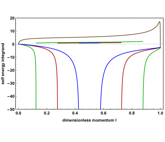
Figure 10: Discontinuities of the integrand over quasimomentum $l$.  The jumps appear at two points, Eq.(49) for all frequencies between the location of the ARPES satellite peak and negative phonon frequency $-\Omega_{s}$.

There are discontinuities at

$$l_{1,2}=\frac{1}{2}\left(1\pm\sqrt{1+4\left(w+\Omega\right)}\right),$$ (49)

when the argument of function $I_{1}\left(a\right)$ equals $1$. The integration was performed in any region separately.

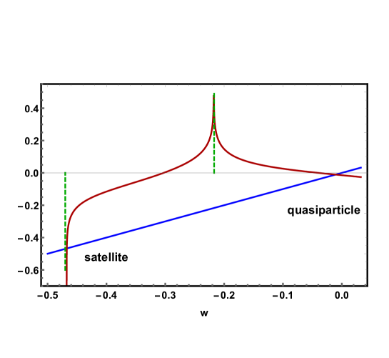
Figure 11: Graphcal soluton of the $w=\Sigma\left(k_{F},w\right)$ equation. Two solutions corresponding to the ARPES satellite peak (negative energy) and the main quasiparticle excitation near zero are apparent.

It is important to note that the discontinuity disappears at $l=1/2$ when $1+4\left(w+\Omega\right)=0$, determining the discontinuity of the integral to be at $w^{-}=-\Omega-1/4$ The equation is solved graphically in Fig. 11 and numerically in Fig. 12  for $\Omega_{h}$ and $\Omega_{s}$. Returning to physical units, for $\Omega_{s}=51.6mev$ one obtains $\omega^{-}=-90.0mev$ with divergence of the spectral weight appearing at $\omega^{peak}=-89.5mev$.

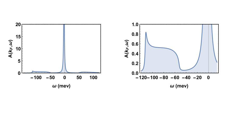
Figure 12: Spectral weight of electron - like excitation. Left: overview of the main quasiparticle and two satellites (ARPES and inverse ARPES).

VI.3 The shape of the quasiparticle satellites

The shape of the spectral weight $A\left(\mathbf{k},\omega\right)$ at $\left|\mathbf{k}\right|=k_{F}$ was calculated for $\Omega=\Omega_{s}$ (see Fig.12, left panel). One observes that beyond the dominant sharp quasiparticle peak near $\omega=0$, there are two small ”satellite” structures created by the soft phonon mode. The one with the spectral weight of $0.13$, observed in ARPES Lee12 ; isotopeGuo , extends (see Fig. 12 right panel) from the phonon mode $\omega=-\Omega_{s}$ all the way to the peak at the satellite location slightly above $\omega=-\Omega_{s}-E_{F}/\hbar\approx-100mev$. The satellite excitation, associated with the hard mode $\Omega_{h}$, would appear at much lower energies and with lower weight.

VI.4 Dimensionless electron - electron coupling $\lambda$

The coupling constant is defined in terms of the self energy analytically continued to the physical frequencies in the limit $\omega\rightarrow 0$)

$$\lambda=-\frac{d}{d\omega}\Sigma\left(k_{F},\omega\right)|_{\omega=0}=\frac{\left(Z_{O}e^{2}\rho\right)^{2}}{8\pi^{2}M\Omega}\int_{l=0}^{2k_{F}}le^{-2l/q_{0}}I_{\lambda}\left(l\right)$$ (50)

One again accounts for the step function $\Theta\left[-\xi_{l,\phi}\right]$ function as $l+2k_{F}\cos\phi<0$, leading to the limiting value of $\phi_{0}=\arccos\left[-l/2k_{F}\right]$:

$$I_{\lambda}\left(l\right) = \int_{\phi=0}^{2\pi}\left(\frac{\Theta\left[-\xi_{l,\phi}\right]}{\left(\xi_{l,\phi}-\Omega\right)^{2}}+\frac{\Theta\left[\xi_{l,\phi}\right]}{\left(\xi_{l,\phi}+\Omega\right)^{2}}\right)$$

$$= \int_{\phi=\phi_{0}}^{\pi}\frac{2}{\left(\frac{l+2k_{F}\cos\phi}{2m^{\ast}}l-\Omega\right)^{2}}+\int_{\phi=0}^{\phi_{0}}\frac{2}{\left(\frac{l+2k_{F}\cos\phi}{2m^{\ast}}l+\Omega\right)^{2}}\text{.}$$

It is important to perform the angle exactly in terms of analytic functions $f_{\lambda}^{1}$, $f_{\lambda}^{2}$ that are somewhat cumbersome. Direct numerical integration suffers from extreme sensitivity near the Fermi level. Changing the variable again to dimensionless $\overline{l}=l/2k_{F}\rightarrow l$, and $\widetilde{\Omega}=\frac{m^{\ast}}{2k_{F}^{2}}\Omega$ one writes,

$$I_{\lambda}\left(l\right)=\frac{m^{\ast 2}}{2k_{F}^{4}l^{2}}\left(f_{\lambda}^{1}\left[l-\widetilde{\Omega}/l\right]+f_{\lambda}^{2}\left[-l-\widetilde{\Omega}/l\right]\right)\text{,}$$ (52)

where

$$f_{\lambda}^{1}\left[a\right] = \frac{1}{a^{2}-1}\left\{\frac{\sqrt{1-l^{2}}}{a+l}+\frac{a}{\sqrt{\left|a^{2}-1\right|}}R^{1}\left[a\right]\right\}$$ (53)

$$f_{\lambda}^{1,2}\left[a\right] = \frac{1}{a^{2}-1}\left\{\frac{\sqrt{1-l^{2}}}{a\mp l}+\frac{a}{\sqrt{\left|a^{2}-1\right|}}R^{1,2}\left[a\right]\right\}$$

$$R^{1}\left[a\right] = \left\{\begin{array}[]{c}2\ \text{arccot}\left[\frac{\sqrt{a^{2}-1}}{a-1}\tan\frac{\phi_{0}}{2}\right]\text{ for }a<-1\\ \text{Re log}\frac{\sqrt{1-a^{2}}\tan\left[\phi_{0}/2\right]+a+1}{\sqrt{1-a^{2}}\tan\left[\phi_{0}/2\right]-a-1}\text{ for }-1<a<-l\end{array}\right|;$$ (56)

$$R^{2}\left[a\right] = \left\{\begin{array}[]{c}2\text{ arctan}\left[\frac{\sqrt{a^{2}-1}}{a-1}\tan\frac{\phi_{0}}{2}\right]\text{ for }a<-1\\ -\text{Re log}\frac{\sqrt{1-a^{2}}\tan\left[\phi_{0}/2\right]+a-1}{\sqrt{1-a^{2}}\tan\left[\phi_{0}/2\right]-a+1}\text{ for }-1<a<-l\end{array}\right|.$$ (59)

The dimensionless coupling constant therefore becomes

$$\lambda=\frac{g^{2}k_{F}^{2}}{\widetilde{\Omega}}\int_{l=0}^{1}\frac{e^{-4k_{F}l/q_{c}}}{l}\left(f_{\lambda}^{1}\left[l-\widetilde{\Omega}/l\right]+f_{\lambda}^{2}\left[-l-\widetilde{\Omega}/l\right]\right)\text{,}$$ (60)

where the electron - phonon coupling definition, Eq.(44) was used. This is convergent (the term in brackets is proportional to $\widetilde{l}$ at small $\widetilde{l}$) and was calculated numerically.  The standard dimensionless electron phonon coupling is from Eq. (52) for the soft and hard modes are $\lambda_{s}=0.23$ and $\lambda_{h}=0.07$ respectively. The first is larger than estimated from the satellite experimentsisotopeGuo , while the second is smaller. However the theoretical formula used in the estimateLee12 ; JohnsonNJP16 ; Kulic was derived on an assumption of delta - like forward scattering peak for the hard mode. The soft mode value alone would not be sufficient, if the BCS formula is applied: $T_{c}=1.14\Omega e^{-1/\lambda_{s}}=9K$. Higher $T_{c}$ value above is caused by the forward peak that is however just exponential, see Eq.(16), much wider than conjectured delta function assumed in ref.Lee12 ; JohnsonNJP16 ; Kulic .

VII Discussion and conclusions.

To summarize, using a microscopic model of the ionic lattice vibrations in the STO substrate below one unit cell $FeSe$, an ”additional” $\Omega_{s}=50mev$ LO interface mode is identified, see Fig.6. The soft mode propagating mainly in the first $TiO_{2}$ layer (”$O$ chains”) has stronger electron - phonon coupling to electron gas in $FeSe$ than a well known $\Omega_{h}=100mev$ hard mode. The increase seem to be solely due to reduced frequency since the matrix elements of the electron - phonon interactions Grimvall ; Eliashberg are very similar for the two modes (numerous other phonon modes DFT16 ; DFTnew have significantly lower matrix elements).

The coupling constant, critical temperature, replica band are calculated. The numerical solution of the gap equations (as well as the Eliashberg approximation to it) results in the $T_{c}=51K$ (while for the ${}^{18}O$ isotope it becomes $T_{c}=49K$). This result is both due to the reduced phonon frequency and due to the spatial separation between the two dimensional electron gas in the $FeSe$ layer and vibrating ions. The later manifests itself in an exponential forward peak in the electron - phonon scattering. It leads to a deviation from the BCS dependence of critical temperature on $\lambda$. The coupling constant, $\lambda=0.23$, is strong enough in this case to account for most if not all of the huge enhancement of the superconductivity on the $STO$ substrate compared to parent compound $FeSe$. The peak is clearly not as sharp as assumed in recent theories Lee12 ; JohnsonNJP16 ; Kulic .

As to remarkable normal state properties of the 1UC $FeSe/STO$, the results are following. The violation of the Migdal theorem is confirmed and satellite excitations due to phonons appear in the spectral weight appear, Fig. 12. The satellite is broad, but unlike in the delta function scattering peak theory Lee12 ; JohnsonNJP16 ; Kulic its divergence appears at frequency much higher than $\Omega_{s}$ consistent with observations. We discuss next possible signatures of the soft mode and generalizations of the mechanism to other high $T_{c}$ materials.

The transversal (TO) counterpart of the LO soft mode considered here indicates a close proximity of the ferroelectric instability of the displacement type due to oxygen ”empty site”, see Fig. 5. Can this be related to known phonon characteristics? Of course $STO$ is a perovskite with very high dielectric constant ”close” to ferroelectric transitionMahan . First the soft surface mode considered here is not related to the displacive structural transitionMahan ; Petzelt in bulk $STO$ at $105K$ (so called $A_{1g}$ mode has large frequencies at low temperature at become soft at $105K$). There exists however another bulk $TO$ modeMahan ; Petzelt ($E_{u}+A_{2u}$), that might be associated with the surface soft mode. Its frequency strongly decreases with temperature and it contributes to the large dielectric constant. Numerous surface measurementsXue16phonon ; phonon and density functional calculationsDFT16 ; DFTnew of phonons in the 1UC $FeSe$/$STO$ system indicate that there are a few possible candidates in the relevant energy domain.

The present approach is a phenomenological in the sense that instead of directly relying on the DFT simulations results for the phonon spectrum, one utilizes the DFT results for the charge distributions in conjunction with the experimental direct studies of the crystalline structure (greatly enhances recently in view of progress in the STM and X rays techniques) in the strongly ionic layers adjacent to 2D electron gas to infer about both the dispersion of the relevant phonon modes and their coupling to charged layer. These are factors that directly affects Cooper pairing. The explicit identification of the dominant degrees of freedom is necessary for a qualitative understanding of the pairing mechanism without the background of plethora of other modes that exist in both the $FeSe$ unit cell and the substrate material. Note that, unlike in other approaches, semi - macroscopic quantities like dielectric constants are included on the microscopic level.

Similar soft modes might exist in other high $T_{c}$ superconductors. For example recently fabricated ultra - thin $CuO_{2}$ films on the $BiO$ surfaces of the $Bi-2212$ crystals were shownXueBSCCO to exhibits large s-wave gap in the $CuO_{2}$ layers. This perovskite allows the microscopic approach outlined in the present work.

Acknowledgements.

We are grateful Prof. Y. Guo, D. Li and L. L.Wang for helpful discussions. Work of B.R. was supported by NSC of R.O.C. Grants No. 98-2112-M-009-014-MY3.

VIII Appendix A. The $TiO_{2}$ oxygen vibration modes

The dominant degree of freedom (oxygen atoms in the interface $TiO_{2}$ on two sublattices directly beneath the $4d$ $Fe$ orbitals) were described in the text. The vibrations along the $z$ direction is also safely neglected. The Hamiltonian for these degrees of freedom is

$$H_{ph}=K_{ph}+W\text{,}$$ (61)

where kinetic energy is

$$K_{ph}=\frac{M}{2}\sum\nolimits_{\mathbf{n}}\left\{\left(\frac{d}{dt}\mathbf{u}_{\mathbf{n}}^{1}\right)^{2}+\left(\frac{d}{dt}\mathbf{u}_{\mathbf{n}}^{2}\right)^{2}\right\}\text{,}$$ (62)

and the potential energy part consists of interatomic potentials defined in Eq.(4) and Table 1. Only interactions of the ”dynamic” oxygen atoms in the $TiO_{2}$ with neighboring $SrO$ below and $Se$ above are taken into account:

$$W = \frac{1}{2}\sum\nolimits_{\mathbf{n,m},A}\left\{v^{TiO}\left[-\mathbf{r}_{\mathbf{m}}^{A}-\mathbf{u}_{\mathbf{m}}^{A}\right]+v^{SrO}\left[\mathbf{R}_{\mathbf{n}}^{Sr}-\mathbf{r}_{\mathbf{m}}^{A}-\mathbf{u}_{\mathbf{m}}^{A}\right]+v^{SeO}\left[\mathbf{R}_{\mathbf{n}}^{Se}-\mathbf{r}_{\mathbf{m}}^{A}-\mathbf{u}_{\mathbf{m}}^{A}\right]+v^{OO}\left[\mathbf{R}_{\mathbf{n}}^{O}-\mathbf{r}_{\mathbf{m}}^{A}-\mathbf{u}_{\mathbf{m}}^{A}\right]\right\}$$

$$+\frac{1}{2}\sum\nolimits_{\mathbf{n\not=m},A}v^{OO}\left[\mathbf{r}_{\mathbf{n}}^{A}-\mathbf{r}_{\mathbf{m}}^{A}+\mathbf{u}_{\mathbf{n}}^{A}-\mathbf{u}_{\mathbf{m}}^{A}\right]+\sum\nolimits_{\mathbf{n,m}}v^{OO}\left[\mathbf{r}_{\mathbf{n}}^{1}-\mathbf{r}_{\mathbf{m}}^{2}+\mathbf{u}_{\mathbf{n}}^{1}-\mathbf{u}_{\mathbf{m}}^{2}\right]\text{.}$$

Here the positions of the heavy $Ti,Sr,Se$ atoms and oxygen atoms of the $SrO$ layer are,

$$\mathbf{R}_{\mathbf{n}}^{Ti} = a\left(n_{x},n_{y},0\right);$$ (64)

$$\mathbf{R}_{\mathbf{n}}^{Sr} = \mathbf{R}_{\mathbf{n}}^{Se}=a\left(n_{x}+\frac{1}{2},n_{y}+\frac{1}{2},z_{Sr}\right);$$

$$\mathbf{R}_{\mathbf{n}}^{O} = a\left(n_{x},n_{y},z_{Sr}\right)\text{,}$$

see Figs. 1-3. Vibrations of heavy atoms and even oxygen in other planes are not expected to be significant due to their mass or distance from the $TiO$ layer oxygen atoms. Some effects of those vibrations is accounted for by the effective oxygen mass, while more remote $Fe$ later above and next $TiO_{2}$ below the important layer were checked to be negligible.

Harmonic approximation consists of expansion around a stable minimum of the energy. The matrix of the second derivatives include:

$$\frac{d^{2}W}{du_{\mathbf{m}}^{\alpha 1}du_{\mathbf{l}}^{\beta 1}} = -\delta_{\mathbf{ml}}\sum\nolimits_{\mathbf{n}}\left\{v_{\alpha\beta}^{TiO}\left[\mathbf{R}_{\mathbf{n}}^{Ti}-\mathbf{r}_{\mathbf{m}}^{1}\right]+v_{\alpha\beta}^{SrO}\left[\mathbf{R}_{\mathbf{n}}^{Sr}-\mathbf{r}_{\mathbf{m}}^{1}\right]+v_{\alpha\beta}^{SeO}\left[\mathbf{R}_{\mathbf{n}}^{Se}-\mathbf{r}_{\mathbf{m}}^{1}\right]+v_{\alpha\beta}^{OO}\left[\mathbf{R}_{\mathbf{n}}^{O}-\mathbf{r}_{\mathbf{m}}^{1}\right]\right\}$$

$$+\delta_{\mathbf{ml}}\sum\nolimits_{\mathbf{n\not=m}}v_{\alpha\beta}^{OO}\left[\mathbf{r}_{\mathbf{m}}^{1}-\mathbf{r}_{\mathbf{n}}^{1}\right]-v_{\alpha\beta}^{OO}\left[\mathbf{r}_{\mathbf{m}}^{1}-\mathbf{r}_{\mathbf{l}}^{1}\right]\sum\nolimits_{\mathbf{n\not=m}}\delta_{\mathbf{nl}}+\delta_{\mathbf{ml}}\sum\nolimits_{\mathbf{n}}v_{\alpha\beta}^{OO}\left[\mathbf{r}_{\mathbf{m}}^{1}-\mathbf{r}_{\mathbf{n}}^{2}\right];$$

$$\frac{d^{2}W}{du_{\mathbf{m}}^{\alpha 1}du_{\mathbf{l}}^{\beta 2}} = -v_{\alpha\beta}^{OO}\left[\mathbf{r}_{\mathbf{m}}^{1}-\mathbf{r}_{\mathbf{l}}^{2}\right];\text{ \ }\frac{d^{2}W}{du_{\mathbf{m}}^{\alpha 2}du_{\mathbf{l}}^{\beta 1}}=-v_{\alpha\beta}^{OO}\left[\mathbf{r}_{\mathbf{m}}^{2}-\mathbf{r}_{\mathbf{l}}^{1}\right];$$

$$\frac{d^{2}W}{du_{\mathbf{m}}^{\alpha 2}du_{\mathbf{l}}^{\beta 2}} = -\delta_{\mathbf{ml}}\sum\nolimits_{\mathbf{n}}\left\{v_{\alpha\beta}^{TiO}\left[\mathbf{R}_{\mathbf{n}}^{Ti}-\mathbf{r}_{\mathbf{m}}^{2}\right]+v_{\alpha\beta}^{SrO}\left[\mathbf{R}_{\mathbf{n}}^{Sr}-\mathbf{r}_{\mathbf{m}}^{2}\right]+v_{\alpha\beta}^{SeO}\left[\mathbf{R}_{\mathbf{n}}^{Se}-\mathbf{r}_{\mathbf{m}}^{2}\right]+v_{\alpha\beta}^{OO}\left[\mathbf{R}_{\mathbf{n}}^{O}-\mathbf{r}_{\mathbf{m}}^{2}\right]\right\}$$

$$+\delta_{\mathbf{ml}}\sum\nolimits_{\mathbf{n\not=m}}v_{\alpha\beta}^{OO}\left[\mathbf{r}_{\mathbf{m}}^{2}-\mathbf{r}_{\mathbf{n}}^{2}\right]+v_{\alpha\beta}\left[\mathbf{r}_{\mathbf{m}}^{2}-\mathbf{r}_{\mathbf{l}}^{2}\right]\sum\nolimits_{\mathbf{n\not=m}}\delta_{\mathbf{nl}}+\delta_{\mathbf{ml}}\sum\nolimits_{\mathbf{n}}v_{\alpha\beta}^{OO}\left[\mathbf{r}_{\mathbf{n}}^{1}-\mathbf{r}_{\mathbf{m}}^{2}\right]\text{.}$$

Here

$$v_{\alpha\beta}^{XY}\left[\mathbf{r}\right]\equiv\frac{d^{2}v^{XY}}{dr_{\alpha}dr_{\beta}}=\frac{e^{2}Z_{X}Z_{Y}}{r^{5}}\left(3r^{\alpha}r^{\beta}-\delta^{\alpha\beta}r^{2}\right)+\frac{\sqrt{A_{X}A_{Y}}b}{r^{3}}\left\{-\delta_{\alpha\beta}r^{2}+r_{\alpha}r_{\beta}\left(1+br\right)\right\}e^{-br}\text{,}$$ (66)

with $b\equiv\frac{1}{2}\left(b^{X}+b^{Y}\right)$.

Fourier transform defined as

$$\mathbf{u}_{\mathbf{k}}^{A}=\frac{1}{N_{s}}\sum\nolimits_{\mathbf{m}}exp\left[-\frac{2\pi yi}{N_{s}}\mathbf{k\cdot m}\right]\mathbf{u}_{\mathbf{m}}^{A}\text{,}$$ (67)

where $N_{s}^{2}$ is the number of unit cells. This leads to the following expression for the dynamic matrix

$$D_{\mathbf{k}}^{\alpha 1\beta 2} = -\frac{1}{N_{s}}\sum\nolimits_{\mathbf{n}}\exp\left[-\frac{2\pi i}{N_{s}}\mathbf{k\cdot n}\right]v_{\alpha\beta}^{OO}\left[\mathbf{r}_{\mathbf{n}}^{1}-\mathbf{r}_{\mathbf{0}}^{2}\right];$$ (68)

$$D_{\mathbf{k}}^{\alpha 2\beta 1} = -\frac{1}{N_{s}}\sum\nolimits_{\mathbf{n}}\exp\left[-\frac{2\pi i}{N_{s}}\mathbf{k\cdot n}\right]v_{\alpha\beta}^{OO}\left[\mathbf{r}_{\mathbf{0}}^{1}-\mathbf{r}_{\mathbf{n}}^{2}\right];$$

$$D_{\mathbf{k}}^{\alpha 1\beta 1} = D_{\mathbf{k}}^{\alpha 2\beta 2}=\frac{1}{N_{s}}\left\{\begin{array}[]{c}\sum\nolimits_{\mathbf{n}}v_{\alpha\beta}^{OO}\left[\mathbf{r}_{\mathbf{n}}^{1}-\mathbf{r}_{\mathbf{0}}^{2}\right]\\ -\sum\nolimits_{\mathbf{n}}\left\{v_{\alpha\beta}^{TiO}\left[\mathbf{R}_{\mathbf{n}}^{Ti}-\mathbf{r}_{\mathbf{0}}^{2}\right]+v_{\alpha\beta}^{SrO}\left[\mathbf{R}_{\mathbf{n}}^{Sr}-\mathbf{r}_{\mathbf{0}}^{2}\right]+v_{\alpha\beta}^{SeO}\left[\mathbf{R}_{\mathbf{n}}^{Se}-\mathbf{r}_{\mathbf{0}}^{2}\right]+v_{\alpha\beta}^{OO}\left[\mathbf{R}_{\mathbf{n}}^{O}-\mathbf{r}_{\mathbf{0}}^{2}\right]\right\}\\ +\sum\nolimits_{\mathbf{n\not=0}}\left(1-\exp\left[-\frac{2\pi i}{N_{s}}\mathbf{k\cdot n}\right]\right)v_{\alpha\beta}^{OO}\left[\mathbf{r}_{\mathbf{n}}^{2}-\mathbf{r}_{\mathbf{0}}^{2}\right]\end{array}\right\}\text{.}$$ (72)

These determine the eigenvalues and polarizations presented in Figs. 5 and Fig. 6 respectively.

IX Appendix B. Derivation of Gorkov equations for a two band system

We derive the Gorkov’s equations within the functional integral approachNO ; frontiers starting from the effective electron action Eqs.(9),(13) for grassmanian fields $\psi_{\mathbf{k},n}^{\ast\sigma A}$ and $\psi_{\mathbf{k},n}^{\sigma A}$:

$$\mathcal{A}\left[\psi\right]=T^{-1}\sum\nolimits_{\mathbf{k}n}\psi_{\mathbf{k}n}^{\ast\sigma A}\left(G_{\mathbf{k}n}^{0}\right)^{-1}\psi_{\mathbf{k}n}^{\sigma A}+\frac{1}{2T}\sum\nolimits_{\mathbf{q}.n}n_{\mathbf{q}n}^{Y}v_{\mathbf{q}n}^{YX}n_{-\mathbf{q,}n}^{X}\text{.}$$ (73)

To simplify the presentation it is useful to lump the quasi - momentum and the Matsubara frequency into a single subscript, $\left\{\mathbf{k},n\right\}\rightarrow\kappa$. In this form (all the repeated indices are assumed to be summed over), the action is:

$$\mathcal{A}\left[\psi\right]=T^{-1}\psi_{\alpha}^{\ast\sigma A}\left(G_{\alpha}^{0}\right)^{-1}\psi_{\alpha}^{\sigma A}+\frac{1}{2T}\psi_{\beta}^{\ast\sigma Y}\psi_{\chi+\beta}^{\sigma Y}v_{\chi}^{YX}\psi_{\gamma}^{\ast\rho X}\psi_{\gamma-\chi}^{\rho X}\text{.}$$ (74)

Functional derivative of the partition sum,

$$Z=\int_{\psi}e^{-\mathcal{A}\left[\psi^{\ast},\psi\right]-J_{\alpha}^{\ast\sigma A}\psi_{\alpha}^{\sigma A}-\psi_{\alpha}^{\ast\sigma A}J_{\alpha}^{\sigma A}}\text{,}$$ (75)

to the following gaussian average of the ”equations of state”,

$$J_{\beta}^{\sigma B} = -\left\langle\frac{\delta\mathcal{A}}{\delta\psi_{\beta}^{\ast\sigma B}}\right\rangle=-\left(G_{\beta}^{0}\right)^{-1}\psi_{\beta}^{\sigma B}+v_{\chi}^{BX}\left\langle\psi_{\gamma}^{\ast\rho X}\psi_{\chi+\beta}^{\sigma B}\right\rangle\psi_{\gamma-\chi}^{\rho X}$$

$$+v_{\chi}^{BX}\left\langle\psi_{\chi+\beta}^{\sigma B}\psi_{\gamma-\chi}^{\rho X}\right\rangle\psi_{\gamma}^{\ast\rho X}-v_{\chi}^{BX}\left\langle\psi_{\gamma}^{\ast\rho X}\psi_{\gamma-\chi}^{\rho X}\right\rangle\psi_{\chi+\beta}^{\sigma B}\text{.}$$

Translation invariance and the s-wave Ansatz,

$$\left\langle\psi_{\mathbf{\beta}}^{\rho B}\psi_{\mathbf{\alpha}}^{\ast\sigma A}\right\rangle = \delta_{\alpha-\beta}\delta^{\sigma\rho}G_{\alpha}^{AB};$$ (77)

$$\left\langle\psi_{\mathbf{\alpha}}^{\sigma A}\psi_{\beta}^{\rho B}\right\rangle = \delta_{\alpha+\beta}\varepsilon^{\sigma\rho}F_{\alpha}^{AB};$$

$$\left\langle\psi_{\mathbf{\alpha}}^{\ast\sigma A}\psi_{\beta}^{\ast\rho B}\right\rangle = \delta_{\alpha+\beta}\varepsilon^{\sigma\rho}F_{\alpha}^{+AB}\text{,}$$

lead lead to:

$$J_{\beta}^{\sigma B}=-\left(G_{\beta}^{0}\right)^{-1}\psi_{\beta}^{\sigma B}-v_{\chi}^{BX}G_{\chi+\beta}^{XB}\psi_{\beta}^{\sigma X}+\varepsilon^{\sigma\rho}v_{\chi}^{BX}F_{\chi+\beta}^{BX}\psi_{\mathbf{-}\beta}^{\ast\rho X}+2v_{0}^{BX}\psi_{\beta}^{\sigma B}G_{\chi}^{XX}\text{.}$$ (78)

Similarly

$$J_{\beta}^{\ast\sigma B} = \left\langle\frac{\delta\mathcal{A}}{\delta\psi_{\beta}^{\sigma B}}\right\rangle=-\left(G_{\beta}^{0}\right)^{-1}\psi_{\beta}^{\ast\sigma B}-v_{\chi}^{BX}\left\langle\psi_{\beta-\chi}^{\ast\sigma B}\psi_{\gamma}^{\ast\rho X}\right\rangle\psi_{\gamma-\chi}^{\rho X}$$

$$+v_{\chi}^{BX}\left\langle\psi_{\beta-\chi}^{\ast\sigma B}\psi_{-\chi+\gamma}^{\rho X}\right\rangle\psi_{\gamma}^{\ast\rho X}-v_{\chi}^{BX}\psi_{\beta-\chi}^{\ast\sigma B}\left\langle\psi_{\gamma}^{\ast\rho X}\psi_{-\chi+\gamma}^{\rho X}\right\rangle$$

$$= \left(G_{\beta}^{0}\right)^{-1}\psi_{\beta}^{\ast\sigma B}-\varepsilon^{\sigma\rho}v_{\chi}^{BX}F_{\beta-\chi}^{+BX}\psi_{-\beta}^{\rho X}-v_{\chi}^{BX}G_{\beta-\chi}^{XB}\psi_{\beta}^{\ast\sigma X}+2v_{0}^{BX}\psi_{\beta}^{\ast\sigma B}G_{\chi}^{XX}\text{.}$$

The second derivatives with respect to fields are${}_{\text{,}}$

$$\frac{\delta J_{\beta}^{\ast\sigma B}}{\delta\psi_{\gamma}^{\rho C}} = -\delta_{\beta+\gamma}\varepsilon^{\sigma\rho}v_{\chi}^{BC}F_{\beta-\chi}^{+BC};$$ (80)

$$\frac{\delta J_{\beta}^{\ast\sigma B}}{\delta\psi_{\gamma}^{\ast\rho C}} = \delta_{\beta-\gamma}\delta^{\sigma\rho}\left(\delta^{BC}\left(G_{\beta}^{0}\right)^{-1}-v_{\chi}^{BC}G_{\beta-\chi}^{CB}-2\delta^{BC}v_{0}^{BX}G_{\chi}^{XX}\right);$$

$$\frac{\delta J_{\beta}^{\sigma B}}{\delta\psi_{\gamma}^{\rho C}} = \delta^{\sigma\rho}\delta_{\beta-\gamma}\left(-\delta^{BC}\left(G_{\beta}^{0}\right)^{-1}-v_{\chi}^{BC}G_{\chi+\beta}^{BC}+2\delta^{BC}v_{0}^{BX}G_{\chi}^{XX}\right);$$

$$\frac{\delta J_{\beta}^{\sigma B}}{\delta\psi_{\gamma}^{\ast\rho C}} = \varepsilon^{\sigma\rho}\delta_{\beta+\gamma}v_{\chi}^{BC}F_{\chi+\beta}^{BC}\text{.}$$

The Gorkov equations are obtained from the following identity

$$\left\langle\psi_{\beta}^{\ast\sigma B}\psi_{\alpha}^{\theta A}\right\rangle\frac{\delta J_{\beta}^{\sigma B}}{\delta\psi_{\gamma}^{\ast\rho C}}+\left\langle\psi_{\alpha}^{\theta A}\psi_{\beta}^{\sigma B}\right\rangle\frac{\delta J_{\beta}^{\ast\sigma B}}{\delta\psi_{\gamma}^{\ast\rho C}} = 0;$$ (81)

$$\left\langle\psi_{\alpha}^{\theta A}\psi_{\beta}^{\ast\sigma B}\right\rangle\frac{\delta J^{\sigma B}}{\delta\psi_{\gamma}^{\rho C}}+\left\langle\psi_{\alpha}^{\theta A}\psi_{\beta}^{\sigma B}\right\rangle\frac{\delta J_{\beta}^{\ast\sigma B}}{\delta\psi^{\rho C}} = \delta^{\theta\rho}\delta^{AC}\text{.}$$

Substituting Eqs.(7780), one finally obtains the first,

$$G_{\alpha}^{CA}\left(G_{\alpha}^{0}\right)^{-1}+\sum\nolimits_{B}G_{\alpha}^{BA}v_{\chi}^{BC}G_{\chi+\alpha}^{BC}-2\sum\nolimits_{X}G_{\alpha}^{CA}v_{0}^{CX}G_{\chi}^{XX}+\sum\nolimits_{B}v_{\chi}^{BC}F_{\alpha}^{AB}F_{-\alpha-\chi}^{+BC}=\delta^{AC}\text{,}$$ (82)

and the second Gorkov equations,

$$F_{\alpha}^{AC}\left(G_{-\alpha}^{0}\right)^{-1}+G_{\alpha}^{BA}v_{\chi}^{BC}F_{\chi+\alpha}^{BC}+F_{\alpha}^{AB}v_{\chi}^{BC}G_{-\alpha-\chi}^{CB}+2F_{\alpha}^{AC}\sum\nolimits_{X}v_{0}^{CX}G_{\chi}^{XX}=0\text{.}$$ (83)

The system of Gorkov equations, Eqs.(82,83) simplifies near the criticality. The last term in Eq.(82) is of order $F^{2}$ and thus negligible. The second and the third terms are small corrections to the normal state Greens function at weak electron - phonon coupling. Therefore one obtains from Eq.(82)

$$G_{\alpha}^{AB}=\delta^{AB}G_{\alpha}^{0}\text{.}$$ (84)

Substituting this into the second Gorkov equation, Eq.(83), one obtains:

$$F_{\alpha}^{AC}+K_{\alpha}^{C}v_{\chi}^{AC}F_{\chi+\alpha}^{AC}=0\text{,}$$ (85)

where

$$K_{\alpha}^{C}=\frac{G_{-\alpha}^{0}G_{\alpha}^{0}}{1+G_{-\alpha}^{0}v_{\chi}^{CC}G_{-\alpha-\chi}^{0}+2G_{-\alpha}^{0}\sum\nolimits_{X}v_{0}^{CX}G_{\chi}^{0}}\text{.}$$ (86)

In the denominator one argues that at weak coupling the first order corrections can be neglected.

X Appendix C. Solution of the gap equation in the Eliashberg approximation

In polar coordinates for an angle independent gap function, $\Delta_{\mathbf{p,}m}^{AC}=\Delta_{k_{F}\mathbf{,}m}^{AC}\equiv\Delta_{m}^{AC}$, and shifting the integration variables as the equation for momentum $\mathbf{q}$ on the Fermi surface, $\varepsilon_{\mathbf{q}}=\varepsilon_{F}$, takes a form:

$$-T_{c}\sum\nolimits_{m}\frac{1}{\left(2\pi\right)^{2}}\int_{\mathbf{l}}\frac{v_{\mathbf{l},n-m}^{AC}}{\left(\omega_{m}^{e}\right)^{2}+\left(\epsilon_{\left|\mathbf{q+l.}\right|}-\epsilon_{F}\right)^{2}}\Delta_{m}^{AC}=\Delta_{n}^{AC}\text{.}$$ (87)

The left hand side of the equation using the fit Eq.(16), can be written in polar coordinates as

$$\frac{T_{c}\left(Z^{O}e^{2}\right)^{2}\rho^{2}}{M\left(2\pi\right)^{2}}\sum\nolimits_{m}\frac{\Delta_{m}^{AC}}{\left(\omega_{n-m}^{b}\right)^{2}+\Omega^{2}}\int_{l=0}^{1/a}le^{-2l/q_{0}}\int_{\phi=0}^{2\pi}\frac{1}{\left(\omega_{m}^{f}\right)^{2}+\xi_{l,\phi}^{2}}\text{,}$$ (88)

Rescaling, $\widetilde{l}=l/2k_{F}$, one obtains:

$$\frac{T_{c}\left(Z_{O}e^{2}\rho m^{\ast}\right)^{2}}{4\pi^{2}Mk_{F}^{2}}\sum\nolimits_{m}\frac{\Delta_{m}^{AC}}{\left(\omega_{n-m}^{b}\right)^{2}+\Omega^{2}}\int_{\widetilde{l}=0}^{1}\frac{e^{-4k_{F}\overline{l}/q_{0}}}{\widetilde{l}}\int_{\phi=0}^{2\pi}\frac{1}{\left(m^{\ast}\omega_{m}^{f}\right)^{2}/\left(2k_{F}^{2}\widetilde{l}\right)^{2}+\left(\overline{l}+\cos\phi\right)^{2}}\text{.}$$ (89)

Integrating exactly over the angle $\phi$,

$$\frac{1}{2\pi}\int_{\phi=0}^{2\pi}\frac{1}{\left(s/l\right)^{2}+\left(l+\cos\phi\right)^{2}}=\frac{l}{s}\text{Re}\left[\left(1+s^{2}/l^{2}-2is-l^{2}\right)^{-1/2}\right]\text{,}$$ (90)

one obtains, dropping tilde over $\widetilde{l}$ in what follows:

$$\frac{\left(Z^{O}e^{2}\rho\right)^{2}m^{\ast}}{\pi^{2}M}\sum\nolimits_{m}\frac{\Delta_{m}^{AC}}{\left(\left(\omega_{n-m}^{b}\right)^{2}+\Omega^{2}\right)\left|2m+1\right|}f\left[\frac{\omega_{m}^{f}m^{\ast}}{2k_{F}^{2}}\right]\text{.}$$ (91)

Here the function is defined as an integral:

$$f\left[z\right]=\int_{l=0}^{1}e^{-4k_{F}l/q_{0}}\text{Re}\left[\frac{1}{\sqrt{1+z^{2}/l^{2}-2iz-l^{2}}}\right]\text{.}$$ (92)

The function $f\left[z\right]$ and its rational fit $f\left[z\right]=0.3\frac{1+z}{1+z+4z^{2}}$ are shown in Fig 13.

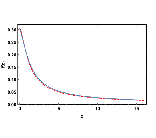
Figure 13: Function $f\left[z\right]$ in the gap equation, Eq.(22) in the main text.

Changing the variables to $\eta_{n}=\sqrt{f\left(\omega_{n}^{f}m^{\ast}/2k_{F}^{2}\right)/\left|\omega_{m}^{f}\right|}\Delta_{n}$, makes the kernel matrix of the integral equation,

$$\sum\nolimits_{m}K_{mn}\eta_{m}=\eta_{n}\text{,}$$ (93)

symmetric,

$$K_{mn}=\frac{\left(\rho Z^{O}e^{2}\right)^{2}m^{\ast}}{\pi^{2}M\left(\left(\omega_{n-m}^{b}\right)^{2}+\Omega^{2}\right)}\sqrt{\frac{f\left(\omega_{m}^{f}m^{\ast}/2k_{F}^{2}\right)f\left(\omega_{n}^{f}m^{\ast}/2k_{F}^{2}\right)}{\left|2m+1\right|\left|2n+1\right|}}\text{.}$$ (94)

Critical temperature is obtained when the largest eigenvalue of the matrix $K$ is unit. This was done numerically by limiting variable $n$ to $\left|n\right|<200$.

Assuming as usualEliashberg , that the dependence of $\Delta$ on $\mathbf{k}$ is weak, $\Delta_{\mathbf{k,}n}^{AB}=\Delta_{n}^{AB}$, substituting the soft mode $v_{\mathbf{l},n-m}^{AC}$ and integrating over polar angle of $l$, the eigenvalue equation simplifies to

$$\frac{\left(Z_{O}e^{2}\rho\right)^{2}m^{\ast}}{\pi^{2}\Omega^{2}M}\sum\nolimits_{m}\frac{f\left[\omega_{m}^{f}m^{\ast}/2k_{F}^{2}\right]}{\left(\left(\omega_{n-m}^{b}/\Omega\right)^{2}+1\right)\left|2m+1\right|}\Delta_{m}^{AC}=\Delta_{n}^{AC}\text{,}$$ (95)

Critical temperature is obtained when the largest eigenvalue of the matrix in Eq.(95) is unit. The numerical results are the following. $T_{c}=51K$, while for isotope ${}^{18}O$ it becomes $T_{c}=49K$.

References

- (1) E. Dagotto, Rev. Mod. Phys. 66, 763 (1994); P. A. Lee, N. Nagaosa, and X.-G.Wen, Rev. Mod. Phys. 78, 17 (2006).
- (2) Q.-Y. Wang, et al, Chin. Phys. Lett. 29, 037402 (2012); D. Liu,et al, Nature Com. 3, 931 (2012); S. He, et al, Nature Mater. 12, 605 (2013); Q. Wang, et al, 2D Mater. 2, 044012 (2015); D. Huang and J. F. Hoffman, Ann. Rev. Cond. Mat. Phys. 8, 311 (2017).
- (3) P. Zhang et al, Phys. Rev. B 94, 104510 (2016).
- (4) S. N. Rebec, T. Jia, C. Zhang, M. Hashimoto, D.H. Lu, R. G. Moore, and Z.X. Shen, Phys. Rev. Lett., 118, 067002 (2017).
- (5) H. Ding, Y.-F. Lv, K. Zhao, W.-L. Wang, L. Wang, C.-L. Song, X. Chen, X.-C. Ma, and Q.-K. Xue. Phys. Rev. Lett., 117, 067001 (2016).
- (6) R. Peng et al, Nature Com. 5, 5044 (2014).
- (7) L. Wang X, Ma, and Q. - K. Xue, Supercond. Sci. Technol. 29, 123001 (2016).
- (8) Y. Zhong et al, Science Bull. 61, 1239 (2016).
- (9) D. - H. Lee, Chinese Physics B 24, 117405 (2015).
- (10) P. Dai, J, Hu, and E. Dagotto, Nat. Phys. 8, 709 (2012).
- (11) M. Z. Shi, N. Z. Wang, B. Lei, C. Shang, F. B. Meng, L. K. Ma, F. X. Zhang, D. Z. Kuang, and X. H. Chen, Phys. Rev. Materials 2, 074801 (2018).
- (12) B. Rosenstein, B.Ya. Shapiro, I. Shapiro, and D. Li, Phys. Rev. B 94, 024505 (2016).
- (13) L. P. Gorkov, Phys. Rev. B 93, 054517, 060507(R) (2016).
- (14) L. Rademaker, Y. Wang, T. Berlijn and T. Johnston, New J. Phys. 18, 022001 (2016)
- (15) M. L. Kulić and O. V. Dolgov, New J. Phys. 19, 013020 (2017).
- (16) Q. Song et al, Nature Com. 10, 758 (2019).
- (17) S. Zhang, J. Guan, X. Jia, B. Liu, W. Wang, F. Li, L. Wang, X. Ma, Q. Xue, J. Zhang, E.W. Plummer, X. Zhu, J. Guo, Phys. Rev. B 94, 081116(R) (2016).
- (18) L. Zhao et al Nature Com. 10, 1038 (2016).
- (19) Y. Y. Xiang, F. Wang, D. Wang, Q. H. Wang, and D. H. Lee, Phys. Rev. B 86, 134508 (2012).
- (20) Y. Wang, K. Nakatsukasa, L. Rademaker, T. Berlijn and S. Johnston, Supercond. Sci. Technol. 29, 054009 (2016).
- (21) M. L. Kulić, Phys. Rep. 38, 1 (2000).
- (22) A. Aperis and P. M. Oppeneer, Phys. Rev. B 97, 060501(R) (2018).
- (23) B. Li, Z. W. Xing, G. Q. Huang, and D. Y. Xing, J. Appl. Phys. 115, 193907 (2014); Y. Xie, H.-Y. Cao, Y. Zhou, S. Chen, H. Xiang, and X.-G. Gong, Sci. Rep. 5, 10011 (2015); Y. Zhou and A. J. Millis, Phys. Rev. B 93, 224506 (2016); Y. N. Huang and W. E. Pickett, Phys. Rev. B 95, 165107 (2017).
- (24) A. A. Abrahamson, Phys. Rev. 178, 76 (1969).
- (25) J. J. Lee et al, Nature 515, 245 (2014).
- (26) R. A. Evarestov, ”Quantum Chemistry of Solids”, Second Edition, Springer Series in Solid-State Sciences 153, Springer, London, 2012.
- (27) L. Wang, X. Ma, and Q. - K. Xue, Supercond. Sci. Technol. 29, 123001 (2016); F. Li, Q. Zhang, C. Tang, C. Liu, J. Shi, C.N. Nie, G. Zhou , Z. Li, W. Zhang, C.-L. Song, 2D materials, 3, 024002 (2016).
- (28) F. Zheng, Z. Wang, W. Kang & P. Zhang, Scientific Rep. 3, 2213 (2013).
- (29) G. M. Eliashberg, ZETF 38, 966 (1960); 39, 1437 (1960) [English translation: Soviet Phys. JETP 11, 696 (1960); 12, 1000 (1961)]; W.L. McMillan, Phys. Rev. 167, 331 (1968).
- (30) G. Grimvall, ”Electron - phonon interactions in metals”, North Holland publishing co, Amsterdam, 1981.
- (31) G. G. Mahan, ”Condensed matter in a nutshell”, Princeton University Press, 2011.
- (32) M.E. Lines and A.M. Glass, Principles and Applications of Ferroelectrics and Related Materials, Claredone Press, Oxford, 2004.
- (33) Q. Fan, et al, Nature Phys., 11, 946 (2015); C. Tang, C. Liu, G. Zhou, F. Li, H. Ding, Z. Li, D. Zhang, Z. Li, C. Song, S. Ji, K. He, L. Wang, X. Ma, Q.K. Xue, Phys. Rev. B 93, 020507(R) (2016).
- (34) S. Zhang, J. Guan, Y. Wang, T. Berlijn, S. Johnston, X. Jia, B. Liu, Q. Zhu, Q. An, S. Xue, Y. Cao, F. Yang, W. Wang, J. Zhang, E.W. Plummer, X. Zhu, J. Guo, Phys. Rev. B 97, 035408 (2018); F. Li and G. A. Sawatzky, Phys. Rev. Let. 120, 237001 (2018).
- (35) Petzelt et al, Phys. Rev. B 64, 184111 (2001).
- (36) J. W. Negele and H. Orland, “Quantum Many-particle Systems”, Perseus Books, 1998; G. Giuliani and G. Vignale,“Quantum Theory of the Electron Liquid”, Cambridge University Press, 2008.
- (37) D. Li, B. Rosenstein, B. Ya Shapiro, and I. Shapiro, Frontiers Phys., 10, 303 (2015).