Fast Convergence of Natural Gradient Descent
for Overparameterized Neural Networks
Abstract
Natural gradient descent has proven effective at mitigating the effects of pathological curvature in neural network optimization, but little is known theoretically about its convergence properties, especially for nonlinear networks. In this work, we analyze for the first time the speed of convergence of natural gradient descent on nonlinear neural networks with squared-error loss. We identify two conditions which guarantee efficient convergence from random initializations: (1) the Jacobian matrix (of network’s output for all training cases with respect to the parameters) has full row rank, and (2) the Jacobian matrix is stable for small perturbations around the initialization. For two-layer ReLU neural networks, we prove that these two conditions do in fact hold throughout the training, under the assumptions of nondegenerate inputs and overparameterization. We further extend our analysis to more general loss functions. Lastly, we show that K-FAC, an approximate natural gradient descent method, also converges to global minima under the same assumptions, and we give a bound on the rate of this convergence.
1 Introduction
Because training large neural networks is costly, there has been much interest in using second-order optimization to speed up training (Becker and LeCun, 1989; Martens, 2010; Martens and Grosse, 2015), and in particlar natural gradient descent (Amari, 1998, 1997). Recently, scalable approximations to natural gradient descent have shown practical success in a variety of tasks and architectures (Martens and Grosse, 2015; Grosse and Martens, 2016; Wu et al., 2017; Zhang et al., 2018a; Martens et al., 2018). Natural gradient descent has an appealing interpretation as optimizing over a Riemannian manifold using an intrinsic distance metric; this implies the updates are invariant to transformations such as whitening (Ollivier, 2015; Luk and Grosse, 2018). It is also closely connected to Gauss-Newton optimization, suggesting it should achieve fast convergence in certain settings (Pascanu and Bengio, 2013; Martens, 2014; Botev et al., 2017).
Does this intuition translate into faster convergence? Amari (1998) provided arguments in the affirmative, as long as the cost function is well approximated by a convex quadratic. However, it remains unknown whether natural gradient descent can optimize neural networks faster than gradient descent — a major gap in our understanding. The problem is that the optimization of neural networks is both nonconvex and non-smooth, making it difficult to prove nontrivial convergence bounds. In general, finding a global minimum of a general non-convex function is an NP-complete problem, and neural network training in particular is NP-complete (Blum and Rivest, 1992).
However, in the past two years, researchers have finally gained substantial traction in understanding the dynamics of gradient-based optimization of neural networks. Theoretically, it has been shown that gradient descent starting from a random initialization is able to find a global minimum if the network is wide enough (Li and Liang, 2018; Du et al., 2018b, a; Zou et al., 2018; Allen-Zhu et al., 2018; Oymak and Soltanolkotabi, 2019). The key technique of those works is to show that neural networks become well-behaved if they are largely overparameterized in the sense that the number of hidden units is polynomially large in the size of the training data. However, most of these works have focused on standard gradient descent, leaving open the question of whether similar statements can be made about other optimizers.
Most convergence analysis of natural gradient descent has focused on simple convex quadratic objectives (e.g. (Martens, 2014)). Very recently, the convergence properties of NGD were studied in the context of linear networks (Bernacchia et al., 2018). While the linearity assumption simplifies the analysis of training dynamics (Saxe et al., 2013), linear networks are severely limited in terms of their expressivity, and it’s not clear which conclusions will generalize from linear to nonlinear networks.
In this work, we analyze natural gradient descent for nonlinear networks. We give two simple and generic conditions on the Jacobian matrix which guarantee efficient convergence to a global minimum. We then apply this analysis to a particular distribution over two-layer ReLU networks which has recently been used to analyze the convergence of gradient descent (Li and Liang, 2018; Du et al., 2018a; Oymak and Soltanolkotabi, 2019). We show that for sufficiently high network width, NGD will converge to the global minimum. We give bounds on the convergence rate of two-layer ReLU networks that are much better than the analogous bounds that have been proven for gradient descent (Du et al., 2018b; Wu et al., 2019; Oymak and Soltanolkotabi, 2019), while allowing for much higher learning rates. Moreover, in the limit of infinite width, and assuming a squared error loss, we show that NGD converges in just one iteration. The main contributions of our work are summarized as follows:
-
•
We provide the first convergence result for natural gradient descent in training randomly-initialized overparameterized neural networks where the number of hidden units is polynomially larger than the number of training samples. We show that natural gradient descent gives an improvement in convergence rate given the same learning rate as gradient descent, where is a Gram matrix that depends on the data.
-
•
We show that natural gradient enables us to use a much larger step size, resulting in an even faster convergence rate. Specifically, the maximal step size of natural gradient descent is for (polynomially) wide networks.
-
•
We show that K-FAC (Martens and Grosse, 2015), an approximate natural gradient descent method, also converges to global minima with linear rate, although this result requires a higher level of overparameterization compared to GD and exact NGD.
-
•
We analyze the generalization properties of NGD, showing that the improved convergence rates provably don’t come at the expense of worse generalization.
2 Related Works
Recently, there have been many works studying the optimization problem in deep learning, i.e., why in practice many neural network architectures reliably converge to global minima (zero training error). One popular way to attack this problem is to analyze the underlying loss surface (Hardt and Ma, 2016; Kawaguchi, 2016; Kawaguchi and Bengio, 2018; Nguyen and Hein, 2017; Soudry and Carmon, 2016). The main argument of those works is that there are no bad local minima. It has been proven that gradient descent can find global minima (Ge et al., 2015; Lee et al., 2016) if the loss surface satisfies: (1) all local minima are global and (2) all saddle points are strict in the sense that there exists at least one negative curvature direction. Unfortunately, most of those works rely on unrealistic assumptions (e.g., linear activations (Hardt and Ma, 2016; Kawaguchi, 2016)) and cannot generalize to practical neural networks. Moreover, Yun et al. (2018) shows that small nonlinearity in shallow networks can create bad local minima.
Another way to understand the optimization of neural networks is to directly analyze the optimization dynamics. Our work also falls within this category. However, most work in this direction focuses on gradient descent. Bartlett et al. ; Arora et al. (2019a) studied the optimization trajectory of deep linear networks and showed that gradient descent can find global minima under some assumptions. Previously, the dynamics of linear networks have also been studied by Saxe et al. (2013); Advani and Saxe (2017). For nonlinear neural networks, a series of papers (Tian, 2017; Brutzkus and Globerson, 2017; Du et al., 2017; Li and Yuan, 2017; Zhang et al., 2018b) studied a specific class of shallow two-layer neural networks together with strong assumptions on input distribution as well as realizability of labels, proving global convergence of gradient descent. Very recently, there are some works proving global convergence of gradient descent (Li and Liang, 2018; Du et al., 2018b, a; Allen-Zhu et al., 2018; Zou et al., 2018; Gao et al., 2019) or adaptive gradient methods (Wu et al., 2019) on overparameterized neural networks. More specifically, Li and Liang (2018); Allen-Zhu et al. (2018); Zou et al. (2018) analyzed the dynamics of weights and showed that the gradient cannot be small if the objective value is large. On the other hand, Du et al. (2018b, a); Wu et al. (2019) studied the dynamics of the outputs of neural networks, where the convergence properties are captured by a Gram matrix. Our work is very similar to Du et al. (2018b); Wu et al. (2019). We note that these papers all require the step size to be sufficiently small to guarantee the global convergence, leading to slow convergence.
To our knowledge, there is only one paper (Bernacchia et al., 2018) studying the global convergence of natural gradient for neural networks. However, Bernacchia et al. (2018) only studied deep linear networks with infinitesimal step size and squared error loss functions. In this sense, our work is the first one proving global convergence of natural gradient descent on nonlinear networks.
There have been many attempts to understand the generalization properties of neural networks since Zhang et al. (2016)’s seminal paper. Researchers have proposed norm-based generalization bounds (Neyshabur et al., 2015, 2017; Bartlett and Mendelson, 2002; Bartlett et al., 2017; Golowich et al., 2017), compression bounds (Arora et al., 2018) and PAC-Bayes bounds (Dziugaite and Roy, 2017, 2018; Zou et al., 2018). Recently, overparameterization of neural networks together with good initialization has been believed to be one key factor of good generalization. Neyshabur et al. (2019) empirically showed that wide neural networks stay close to the initialization, thus leading to good generalization. Theoretically, researchers did prove that overparameterization as well as linear convergence jointly restrict the weights to be close to the initialization (Du et al., 2018b, a; Allen-Zhu et al., 2018; Zou et al., 2018; Arora et al., 2019b). The most closely related paper is Arora et al. (2019b), which shows that the optimization and generalization phenomenon can be explained by a Gram matrix. The main difference is that our analysis is based on natural gradient descent, which converges faster and provably generalizes as well as gradient descent.
Concurrently and independently, Cai et al. (2019) showed that natural gradient descent (they call it Gram-Gauss-Newton) enjoys quadratic convergence rate guarantee for overparameterized networks on regression problems. Additionally, they showed that it is much cheaper to precondition the gradient in the output space when the number of data points is much smaller than the number of parameters.
3 Convergence Analysis of Natural Gradient Descent
We begin our convergence analysis of natural gradient descent – under appropriate conditions – for the neural network optimization problem. Formally, we consider a generic neural network with a single output and squared error loss for simplicity111It is easy to extend to multi-output networks and other loss functions, here we focus on single-output and quadratic just for notational simplicity., where denots all parameters of the network (i.e. weights and biases). Given a training dataset , we want to minimize the following loss function:
| (1) |
One main focus of this paper is to analyze the following procedure:
| (2) |
where is the step size, and is the Fisher information matrix associated with the network’s predictive distribution over (which is implied by its loss function and is for the squared error loss) and the dataset’s distribution over .
As shown by Martens (2014), the Fisher is equivalent to the generalized Gauss-Newton matrix, defined as if the predictive distribution is in the exponential family, such as categorical distribution (for classification) or Gaussian distribution (for regression). is the Jacobian matrix of with respect to the parameters and is the Hessian of the loss with respect to the network prediction (which is in our setting). Therefore, with the squared error loss, the Fisher matrix can be compactly written as (which coincides with classical Gauss-Newton matrix), where is the Jacobian matrix for the whole dataset. In practice, when the number of parameters is larger than number of samples we have, the Fisher information matrix is surely singular. In that case, we take the generalized inverse (Bernacchia et al., 2018) with , which gives the following update rule:
| (3) |
where and .
We now introduce two conditions on the network that suffice for proving the global convergence of NGD to a minimizer which achieves zero training loss (and is therefore a global minimizer). To motivate these two conditions we make the following observations. First, the global minimizer is characterized by the condition that the gradient in the output space is zero for each case (i.e. ). Meanwhile, local minima are characterized by the condition that the gradient with respect to the parameters is zero. Thus, one way to avoid finding local minima that aren’t global is to ensure that the parameter gradient is zero if and only if the output space gradient (for each case) is zero. It’s not hard to see that this property holds as long as remains non-singular throughout optimization (or equivalently that always has full row rank). The following two conditions ensure that this happens, by first requiring that this property hold at initialization time, and second that changes slowly enough that it remains true in a big enough neighborhood around .
Condition 1 (Full row rank of Jacobian matrix).
The Jacobian matrix at the initialization has full row rank, or equivalently, the Gram matrix is positive definite.
Remark 1.
Condition 1 implies that , which means the Fisher information matrix is singular and we have to use the generalized inverse except in the case where .
Condition 2 (Stable Jacobian).
There exists such that for all parameters that satisfy , we have
| (4) |
This condition shares the same spirit with the Lipschtiz smoothness assumption in classical optimization theory. It implies (with small ) that the network is close to a linearized network (Lee et al., 2019) around the initialization and therefore natural gradient descent update is close to the gradient descent update in the output space. Along with Condition 1, we have the following theorem.
Theorem 1 (Natural gradient descent).
To be noted, is the squared error loss up to a constant. Due to space constraints we only give a short sketch of the proof here. The full proof is given in Appendix B.
Proof Sketch. Our proof relies on the following insights. First, if the Jacobian matrix has full row rank, this guarantees linear convergence for infinitesimal step size. The linear convergence property restricts the parameters to be close to the initialization, which implies the Jacobian matrix is always full row rank throughout the training, and therefore natural gradient descent with infinitesimal step size converges to global minima. Furthermore, given the network is close to a linearized network (since the Jacobian matrix is stable with respect to small perturbations around the initialization), we are able to extend the proof to discrete time with a large step size.
In summary, we prove that NGD exhibits linear convergence to the global minimizer of the neural network training problem, under Conditions 1 and 2. We believe our arguments in this section are general (i.e., architecture-agnostic), and can serve as a recipe for proving global convergence of natural gradient descent in other settings.
3.1 Other Loss Functions
We note that our analysis can be easily extended to more general loss function class. Here, we take the class of functions that are -strongly convex with -Lipschitz gradients as an example. Note that strongly convexity is a very mild assumption since we can always add regularization to make the convex loss strongly convex. Therefore, this function class includes regularized cross-entropy loss (which is typically used in classification) and squared error (for regression). For this type of loss, we need a strong version of Condition 2.
Condition 3 (Stable Jacobian).
There exists such that for all parameters that satisfy where
| (6) |
Theorem 2.
The key step of proving Theorem 2 is to show if is large enough, then natural gradient descent is approximately gradient descent in the output space. Thus the results can be easily derived according to standard bounds for convex optimization. Due to the page limit, we defer the proof to the Appendix C.
Remark 2.
In Theorem 2, the convergence rate depends on the condition number , which can be removed if we take into the curvature information of the loss function. In other words, we expect that the bound has no dependency on if we use the Fisher matrix rather than the classical Gauss-Newton (assuming Euclidean metric in the output space (Luk and Grosse, 2018)) in Theorem 2.
4 Optimizing Overparameterized Neural Networks
In Section 3, we analyzed the convergence properties of natural gradient descent, under the abstract Conditions 1 and 2. In this section, we make our analysis concrete by applying it to a specific type of overparameterized network (with a certain random initialization). We show that Conditions 1 and 2 hold with high probability. We therefore establish that NGD exhibits linear convergence to a global minimizer for such networks.
4.1 Notation
We let . We use , to denote the Kronecker and Hadamard products. And we use and to denote row-wise and column-wise Khatri-Rao products, respectively. For a matrix , we use to denote its -th entry. We use to denote the Euclidean norm of a vector or spectral norm of a matrix and to denote the Frobenius norm of a matrix. We use and to denote the largest and smallest eigenvalue of a square matrix, and and to denote the largest and smallest singular value of a (possibly non-square) matrix. For a positive definite matrix , we use to denote its condition number, i.e., . We also use to denote the standard inner product between two vectors. Given an event , we use to denote the indicator function for .
4.2 Problem Setup
Formally, we consider a neural network of the following form:
| (8) |
where is the input, is the weight matrix (formed into a vector) of the first layer, is the output weight of hidden unit and is the ReLU activation function (acting entry-wise for vector arguments). For , we initialize the weights of first layer and output weight .
Assumption 1.
For all i, and . For any , .
This very mild condition simply requires the inputs and outputs have standardized norms, and that different input vectors are distinguishable from each other. Datasets that do not satisfy this condition can be made to do so via simple pre-processing.
Following Du et al. (2018b); Oymak and Soltanolkotabi (2019); Wu et al. (2019), we only optimize the weights of the first layer222We fix the second layer just for simplicity. Based on the same analysis, one can also prove global convergence for jointly training both layers., i.e., . Therefore, natural gradient descent can be simplified to
| (9) |
Though this is only a shallow fully connected neural network, the objective is still non-smooth and non-convex (Du et al., 2018b) due to the use of ReLU activation function. We further note that this two-layer network model has been useful in understanding the optimization and generalization of deep neural networks (Xie et al., 2016; Li and Liang, 2018; Du et al., 2018b; Arora et al., 2019b; Wu et al., 2019), and some results have been extended to multi-layer networks (Du et al., 2018a).
Definition 1 (Limiting Gram Matrix).
The limiting Gram matrix is defined as follows. For - entry, we have
| (10) |
This matrix coincides with neural tangent kernel (Jacot et al., 2018) for ReLU activation function. As shown by Du et al. (2018b), this matrix is positive definite and we define its smallest eigenvalue . In the same way, we can define its finite version with -entry .
4.3 Exact Natural Gradient Descent
In this subsection, we present our result for this setting. The main difficulty is to show that Conditions 1 and 2 hold. Here we state our main result.
Theorem 3 (Natural Gradient Descent for overparameterized Networks).
Under Assumption 1, if we i.i.d initialize , for , we set the number of hidden nodes , and the step size , then with probability at least over the random initialization we have for
| (11) |
Even though the objective is non-convex and non-smooth, natural gradient descent with a constant step size enjoys a linear convergence rate. For large enough , we show that the learning rate can be chosen up to , so NGD can provably converge within steps. Compared to analogous bounds for gradient descent (Du et al., 2018a; Oymak and Soltanolkotabi, 2019; Wu et al., 2019), we improve the maximum allowable learning rate from to and also get rid of the dependency on . Overall, NGD (Theorem 3) gives an improvement over gradient descent.
Our strategy to prove this result will be to show that for the given choice of random initialization, Condition 1 and 2 hold with high probability. For proving Condition 1 hold, we used matrix concentration inequalities. For Condition 2, we show that , which implies the Jacobian is stable for wide networks. For detailed proof, we refer the reader to the Appendix D.1.
4.4 Approximate Natural Gradient Descent with K-FAC
Exact natural gradient descent is quite expensive in terms of computation or memory. In training deep neural networks, K-FAC (Martens and Grosse, 2015) has been a powerful optimizer for leveraging curvature information while retaining tractable computation. The K-FAC update rule for the two-layer ReLU network is given by
| (12) |
where denotes the matrix formed from the input vectors (i.e. ), and is the matrix of pre-activation derivatives. Under the same argument as the Gram matrix , we get that is strictly positive definite with smallest eigenvalue (see Appendix D.3 for detailed proof).
We show that for sufficiently wide networks, K-FAC does converge linearly to a global minimizer. We further show, with a particular transformation on the input data, K-FAC does match the optimization performance of exact natural gradient for two-layer ReLU networks. Here we state the main result.
Theorem 4 (K-FAC).
Under the same assumptions as in Theorem 3, plus the additional assumption that , if we set the number of hidden units and step size , then with probability at least over the random initialization, we have for
| (13) |
The key step in proving Theorem 4 is to show
| (14) |
Remark 3.
Remark 4.
The dependence of the convergence rate on in Theorem 4 may seem paradoxical, as K-FAC is invariant to invertible linear transformations of the data (including those that would change ). But we note that said transformations would also make the norms of the input vectors non-uniform, thus violating Assumption 1 in a way that isn’t repairable. Interestingly, there exists an invertible linear transformation which, if applied to the input vectors and followed by normalization, produces vectors that simultaneously satisfy Assumption 1 and the condition (thus improving the bound in Theorem 4 substantially). See Appendix A for details. Notably, K-FAC is not invariant to such pre-processing, as the normalization step is a nonlinear operation.
To quantify the degree of overparameterization (which is a function of the network width ) required to achieve global convergence under our analysis, we must estimate . To this end, we observe that , and then apply the following lemma:
Lemma 1.
[Schur (1911)] For two positive definite matrices and , we have
| (15) | ||||
The diagonal entries of are all since the inputs are normalized. Therefore, we have according to Lemma 1, and hence K-FAC requires a slightly higher degree of overparameterization than exact NGD under our analysis.
4.5 Bounding
As pointed out by Allen-Zhu et al. (2018), it is unclear if is small or even polynomial. Here, we bound using matrix concentration inequalities and harmonic analysis. To leverage harmonic analysis, we have to assume the data are drawn i.i.d. from the unit sphere333This assumption is not too stringent since the inputs are already normalized. Moreover, we can relax the assumption of unit sphere input to separable input, which is used in Li and Liang (2018); Allen-Zhu et al. (2018); Zou et al. (2018). See Oymak and Soltanolkotabi (2019) (Theorem I.1) for more details..
Theorem 5.
Under this assumption on the training data, with probability ,
| (16) |
Basically, Theorem 5 says that the Gram matrix should have high chance of having large smallest eigenvalue if the training data are uniformly distributed. Intuitively, we would expect the smallest eigenvalue to be very small if all are similar to each other. Therefore, some notion of diversity of the training inputs is needed. We conjecture that the smallest eigenvalue would still be large if the data are -separable (i.e., for any pair ), an assumption adopted by Li and Liang (2018); Allen-Zhu et al. (2018); Zou et al. (2018).
5 Generalization analysis
It is often speculated that NGD or other preconditioned gradient descent methods (e.g., Adam) perform worse than gradient descent in terms of generalization (Wilson et al., 2017). In this section, we show that NGD achieves the same generalization bounds which have been proved for GD, at least for two-layer ReLU networks.
Consider a loss function . The expected risk over the data distribution and the empirical risk over a training set are defined as
| (17) |
It has been shown (Neyshabur et al., 2019) that the Redemacher complexity (Bartlett and Mendelson, 2002) for two-layer ReLU networks depends on . By the standard Rademacher complexity generalization bound, we have the following bound (see Appendix E.1 for proof):
Theorem 6.
Given a target error parameter and failure probability . Suppose and . For any 1-Lipschitz loss function, with probability at least over random initialization and training samples, the two-layer neural network trained by NGD for iterations has expected loss bounded as:
| (18) |
6 Conclusion
We’ve analyzed for the first time the rate of convergence to a global optimum for (both exact and approximate) natural gradient descent on nonlinear neural networks. Particularly, we identified two conditions which guarantee the global convergence, i.e., the Jacobian matrix with respect to the parameters has full row rank and stable for perturbations around the initialization. Based on these insights, we improved the convergence rate of gradient descent by a factor of on two-layer ReLU networks by using natural gradient descent. Beyond that, we also showed that the improved convergence rates don’t come at the expense of worse generalization.
Acknowledgements
We thank Jeffrey Z. HaoChen, Shengyang Sun and Mufan Li for helpful discussion.
References
- Advani and Saxe (2017) Madhu S Advani and Andrew M Saxe. High-dimensional dynamics of generalization error in neural networks. arXiv preprint arXiv:1710.03667, 2017.
- Allen-Zhu et al. (2018) Zeyuan Allen-Zhu, Yuanzhi Li, and Zhao Song. A convergence theory for deep learning via over-parameterization. arXiv preprint arXiv:1811.03962, 2018.
- Amari (1997) Shun-ichi Amari. Neural learning in structured parameter spaces-natural riemannian gradient. In Advances in neural information processing systems, pages 127–133, 1997.
- Amari (1998) Shun-Ichi Amari. Natural gradient works efficiently in learning. Neural computation, 10(2):251–276, 1998.
- Arora et al. (2018) Sanjeev Arora, Rong Ge, Behnam Neyshabur, and Yi Zhang. Stronger generalization bounds for deep nets via a compression approach. arXiv preprint arXiv:1802.05296, 2018.
- Arora et al. (2019a) Sanjeev Arora, Nadav Cohen, Noah Golowich, and Wei Hu. A convergence analysis of gradient descent for deep linear neural networks. In International Conference on Learning Representations, 2019a. URL https://openreview.net/forum?id=SkMQg3C5K7.
- Arora et al. (2019b) Sanjeev Arora, Simon S Du, Wei Hu, Zhiyuan Li, and Ruosong Wang. Fine-grained analysis of optimization and generalization for overparameterized two-layer neural networks. arXiv preprint arXiv:1901.08584, 2019b.
- Bartlett and Mendelson (2002) Peter L Bartlett and Shahar Mendelson. Rademacher and gaussian complexities: Risk bounds and structural results. Journal of Machine Learning Research, 3(Nov):463–482, 2002.
- (9) Peter L Bartlett, David P Helmbold, and Philip M Long. Gradient descent with identity initialization efficiently learns positive-definite linear transformations by deep residual networks. Neural computation, pages 1–26.
- Bartlett et al. (2017) Peter L Bartlett, Dylan J Foster, and Matus J Telgarsky. Spectrally-normalized margin bounds for neural networks. In Advances in Neural Information Processing Systems, pages 6240–6249, 2017.
- Becker and LeCun (1989) S. Becker and Y. LeCun. Improving the convergence of backpropagation learning with second order methods. In Proceedings of the 1988 Connectionist Models Summer School, 1989.
- Bernacchia et al. (2018) Alberto Bernacchia, Mate Lengyel, and Guillaume Hennequin. Exact natural gradient in deep linear networks and its application to the nonlinear case. In Advances in Neural Information Processing Systems, pages 5945–5954, 2018.
- Blum and Rivest (1992) Avrim Blum and Ronald L. Rivest. Training a 3-node neural network is np-complete. Neural Networks, 5:117–127, 1992.
- Botev et al. (2017) Aleksandar Botev, Hippolyt Ritter, and David Barber. Practical Gauss-Newton optimisation for deep learning. In International Conference on Machine Learning, 2017.
- Boyd and Vandenberghe (2004) Stephen Boyd and Lieven Vandenberghe. Convex optimization. Cambridge university press, 2004.
- Brutzkus and Globerson (2017) Alon Brutzkus and Amir Globerson. Globally optimal gradient descent for a convnet with gaussian inputs. In Proceedings of the 34th International Conference on Machine Learning-Volume 70, pages 605–614. JMLR. org, 2017.
- Cai et al. (2019) Tianle Cai, Ruiqi Gao, Jikai Hou, Siyu Chen, Dong Wang, Di He, Zhihua Zhang, and Liwei Wang. A gram-gauss-newton method learning overparameterized deep neural networks for regression problems. arXiv preprint arXiv:1905.11675, 2019.
- Du et al. (2017) Simon S Du, Jason D Lee, and Yuandong Tian. When is a convolutional filter easy to learn? arXiv preprint arXiv:1709.06129, 2017.
- Du et al. (2018a) Simon S Du, Jason D Lee, Haochuan Li, Liwei Wang, and Xiyu Zhai. Gradient descent finds global minima of deep neural networks. arXiv preprint arXiv:1811.03804, 2018a.
- Du et al. (2018b) Simon S Du, Xiyu Zhai, Barnabas Poczos, and Aarti Singh. Gradient descent provably optimizes over-parameterized neural networks. arXiv preprint arXiv:1810.02054, 2018b.
- Dziugaite and Roy (2017) Gintare Karolina Dziugaite and Daniel M Roy. Computing nonvacuous generalization bounds for deep (stochastic) neural networks with many more parameters than training data. arXiv preprint arXiv:1703.11008, 2017.
- Dziugaite and Roy (2018) Gintare Karolina Dziugaite and Daniel M Roy. Data-dependent pac-bayes priors via differential privacy. In Advances in Neural Information Processing Systems, pages 8440–8450, 2018.
- Forster (2002) Jürgen Forster. A linear lower bound on the unbounded error probabilistic communication complexity. Journal of Computer and System Sciences, 65(4):612–625, 2002.
- Gao et al. (2019) Weihao Gao, Ashok Makkuva, Sewoong Oh, and Pramod Viswanath. Learning one-hidden-layer neural networks under general input distributions. In The 22nd International Conference on Artificial Intelligence and Statistics, pages 1950–1959, 2019.
- Ge et al. (2015) Rong Ge, Furong Huang, Chi Jin, and Yang Yuan. Escaping from saddle points—online stochastic gradient for tensor decomposition. In Conference on Learning Theory, pages 797–842, 2015.
- Golowich et al. (2017) Noah Golowich, Alexander Rakhlin, and Ohad Shamir. Size-independent sample complexity of neural networks. arXiv preprint arXiv:1712.06541, 2017.
- Grosse and Martens (2016) Roger Grosse and James Martens. A Kronecker-factored approximate Fisher matrix for convolution layers. In International Conference on Machine Learning, 2016.
- Hardt and Ma (2016) Moritz Hardt and Tengyu Ma. Identity matters in deep learning. arXiv preprint arXiv:1611.04231, 2016.
- Jacot et al. (2018) Arthur Jacot, Franck Gabriel, and Clément Hongler. Neural tangent kernel: Convergence and generalization in neural networks. In Advances in neural information processing systems, pages 8580–8589, 2018.
- Kawaguchi (2016) Kenji Kawaguchi. Deep learning without poor local minima. In Advances in neural information processing systems, pages 586–594, 2016.
- Kawaguchi and Bengio (2018) Kenji Kawaguchi and Yoshua Bengio. Depth with nonlinearity creates no bad local minima in resnets. arXiv preprint arXiv:1810.09038, 2018.
- LeCun et al. (1998) Yann LeCun, Léon Bottou, Yoshua Bengio, Patrick Haffner, et al. Gradient-based learning applied to document recognition. Proceedings of the IEEE, 86(11):2278–2324, 1998.
- Lee et al. (2019) Jaehoon Lee, Lechao Xiao, Samuel S Schoenholz, Yasaman Bahri, Jascha Sohl-Dickstein, and Jeffrey Pennington. Wide neural network of any depth evolve as linear models under gradient descent. arXiv preprint arXiv:1902.06720, 2019.
- Lee et al. (2016) Jason D Lee, Max Simchowitz, Michael I Jordan, and Benjamin Recht. Gradient descent converges to minimizers. arXiv preprint arXiv:1602.04915, 2016.
- Li and Liang (2018) Yuanzhi Li and Yingyu Liang. Learning overparameterized neural networks via stochastic gradient descent on structured data. In Advances in Neural Information Processing Systems, pages 8168–8177, 2018.
- Li and Yuan (2017) Yuanzhi Li and Yang Yuan. Convergence analysis of two-layer neural networks with relu activation. In Advances in Neural Information Processing Systems, pages 597–607, 2017.
- Luk and Grosse (2018) Kevin Luk and Roger Grosse. A coordinate-free construction of scalable natural gradient. arXiv preprint arXiv:1808.1340, 2018.
- Martens (2010) James Martens. Deep learning via hessian-free optimization. In ICML, volume 27, pages 735–742, 2010.
- Martens (2014) James Martens. New insights and perspectives on the natural gradient method. arXiv preprint arXiv:1412.1193, 2014.
- Martens and Grosse (2015) James Martens and Roger Grosse. Optimizing neural networks with kronecker-factored approximate curvature. In International conference on machine learning, pages 2408–2417, 2015.
- Martens et al. (2018) James Martens, Jimmy Ba, and Matt Johnson. Kronecker-factored curvature approximations for recurrent neural networks. In International Conference on Learning Representations, 2018.
- Mohri et al. (2018) Mehryar Mohri, Afshin Rostamizadeh, and Ameet Talwalkar. Foundations of machine learning. 2018.
- Neyshabur et al. (2015) Behnam Neyshabur, Ryota Tomioka, and Nathan Srebro. Norm-based capacity control in neural networks. In Conference on Learning Theory, pages 1376–1401, 2015.
- Neyshabur et al. (2017) Behnam Neyshabur, Srinadh Bhojanapalli, and Nathan Srebro. A pac-bayesian approach to spectrally-normalized margin bounds for neural networks. arXiv preprint arXiv:1707.09564, 2017.
- Neyshabur et al. (2019) Behnam Neyshabur, Zhiyuan Li, Srinadh Bhojanapalli, Yann LeCun, and Nathan Srebro. The role of over-parametrization in generalization of neural networks. In International Conference on Learning Representations, 2019. URL https://openreview.net/forum?id=BygfghAcYX.
- Nguyen and Hein (2017) Quynh Nguyen and Matthias Hein. The loss surface of deep and wide neural networks. In Proceedings of the 34th International Conference on Machine Learning-Volume 70, pages 2603–2612. JMLR. org, 2017.
- Ollivier (2015) Yann Ollivier. Riemannian metrics for neural networks I: Feedforward networks. Information and Inference, 4:108–153, 2015.
- Oymak and Soltanolkotabi (2019) Samet Oymak and Mahdi Soltanolkotabi. Towards moderate overparameterization: global convergence guarantees for training shallow neural networks. arXiv preprint arXiv:1902.04674, 2019.
- Pascanu and Bengio (2013) Razvan Pascanu and Yoshua Bengio. Revisiting natural gradient for deep networks. arXiv preprint arXiv:1301.3584, 2013.
- Saxe et al. (2013) Andrew M Saxe, James L McClelland, and Surya Ganguli. Exact solutions to the nonlinear dynamics of learning in deep linear neural networks. arXiv preprint arXiv:1312.6120, 2013.
- Schur (1911) Jssai Schur. Bemerkungen zur theorie der beschränkten bilinearformen mit unendlich vielen veränderlichen. Journal für die reine und Angewandte Mathematik, 140:1–28, 1911.
- Soudry and Carmon (2016) Daniel Soudry and Yair Carmon. No bad local minima: Data independent training error guarantees for multilayer neural networks. arXiv preprint arXiv:1605.08361, 2016.
- Tian (2017) Yuandong Tian. An analytical formula of population gradient for two-layered relu network and its applications in convergence and critical point analysis. In Proceedings of the 34th International Conference on Machine Learning-Volume 70, pages 3404–3413. JMLR. org, 2017.
- Tropp et al. (2015) Joel A Tropp et al. An introduction to matrix concentration inequalities. Foundations and Trends® in Machine Learning, 8(1-2):1–230, 2015.
- Wilson et al. (2017) Ashia C Wilson, Rebecca Roelofs, Mitchell Stern, Nati Srebro, and Benjamin Recht. The marginal value of adaptive gradient methods in machine learning. In Advances in Neural Information Processing Systems, pages 4148–4158, 2017.
- Wu et al. (2019) Xiaoxia Wu, Simon S Du, and Rachel Ward. Global convergence of adaptive gradient methods for an over-parameterized neural network. arXiv preprint arXiv:1902.07111, 2019.
- Wu et al. (2017) Yuhuai Wu, Elman Mansimov, Shun Liao, Roger Grosse, and Jimmy Ba. Scalable trust-region method for deep reinforcement learning using Kronecker-factored approximation. In Neural Information Processing Systems, 2017.
- Xie et al. (2016) Bo Xie, Yingyu Liang, and Le Song. Diverse neural network learns true target functions. arXiv preprint arXiv:1611.03131, 2016.
- Yun et al. (2018) Chulhee Yun, Suvrit Sra, and Ali Jadbabaie. Small nonlinearities in activation functions create bad local minima in neural networks. arXiv preprint arXiv:1802.03487, 2018.
- Zhang et al. (2016) Chiyuan Zhang, Samy Bengio, Moritz Hardt, Benjamin Recht, and Oriol Vinyals. Understanding deep learning requires rethinking generalization. arXiv preprint arXiv:1611.03530, 2016.
- Zhang et al. (2018a) Guodong Zhang, Shengyang Sun, David Duvenaud, and Roger Grosse. Noisy natural gradient as variational inference. In International Conference on Machine Learning, pages 5847–5856, 2018a.
- Zhang et al. (2018b) Xiao Zhang, Yaodong Yu, Lingxiao Wang, and Quanquan Gu. Learning one-hidden-layer relu networks via gradient descent. arXiv preprint arXiv:1806.07808, 2018b.
- Zou et al. (2018) Difan Zou, Yuan Cao, Dongruo Zhou, and Quanquan Gu. Stochastic gradient descent optimizes over-parameterized deep relu networks. arXiv preprint arXiv:1811.08888, 2018.
Appendix A The Forster Transform
In a breakthrough paper in the area of communication complexity, Forster [2002] used the existence of a certain kind of dataset transformation as the key technical tool in the proof of his main result. The Theorem which establishes the existence of this transformation is paraphrased below.
Theorem 7 (Forster [2002], Theorem 4.1).
Suppose is a matrix such that all subsets of size at most of its rows are linearly independent. Then there exists an invertible matrix such that if we post-multiply by (i.e. apply to each row), and then normalize each row by its 2-norm, the resulting matrix satisfies .
Remark 5.
Note that the technical condition about linear independence can be easily be made to hold for an arbitrary by adding an infinitesimal random perturbation, assuming it doesn’t hold to begin with.
This result basically says that for any set of vectors, there is a linear transformation of said vectors which makes their normalized versions (given by the rows of ) satisfy . So by combining this linear transformation with normalization we produce a set of vectors that simultaneously satisfy Assumption 1, while also satisfying .
Forster’s proof of Theorem 7 can be interpreted as defining a transformation function on (initialized at ), and showing that it has a fixed point with the required properties. One can derive an algorithm from this by repeatedly applying the transformation to , which consists of "whitening" followed by normalization, until is sufficiently close to . The matrix is then simply the product of the "whitening" transformation matrices, up to a scalar constant. While no explicit finite-time convergence guarantees are given for this algorithm by Forster [2002], we have implemented it and verified that it does indeed converge at a reasonable rate. The algorithm is outlined below.
Appendix B Proof of Theorem 1
We prove the result in two steps: we first provide a convergence analysis for natural gradient flow, i.e., natural gradient descent with infinitesimal step size, and then take into account the error introduced by discretization and show global convergence for natural gradient descent.
To guarantee global convergence for natural gradient flow, we only need to show that the Gram matrix is positive definite throughout the training. Intuitively, for successfully finding global minima, the network must satisfy the following condition, i.e., the gradient with respect to the parameters is zero only if the gradient in the output space is zero. It suffices to show that the Gram matrix is positive definite, or equivalently, the Jacobian matrix is full row rank.
By Condition 1 and Condition 2, we immediately obtain the following lemma that if the parameters stay close to the initialization, then the Gram matrix is positive definite throughout the training.
Lemma 2.
If , then we have .
Proof of Lemma 2.
Based on the inequality that where denotes singular value, we have
| (19) |
By Condition 2, we have , thus we get which completes the proof. ∎
With the assumption that throughout the training, we are now ready to prove global convergence for natural gradient flow. Recall the dynamics of natural gradient flow in weight space,
| (20) |
Accordingly, we can calculate the dynamics of the network predictions.
| (21) | ||||
Since the Gram matrix is positive definite, its inverse does exist. Therefore, we have
| (22) |
By the chain rule, we get the dynamics of the loss in the following form:
| (23) |
By integrating eqn. (23), we find that .
That completes the continuous time analysis, under the assumption that the parameters stay close to the initialization. The discrete case follows similarly, except that we need to account for the discretization error. Analogously to eqn. (21), we calculate the difference of predictions between two consecutive iterations.
| (24) | ||||
where we have defined .
Next we bound the norm of the second term () in the RHS of eqn. (24). Using Condition 2 and Lemma 2 we have that
| (25) | ||||
In the first inequality, we used the fact (based on Condition 2) that
| (26) | ||||
Lastly, we have
| (27) | ||||
In the last inequality of eqn. (27), we use the assumption that .
So far, we have assumed the parameters fall within a certain radius around the initialization. We now justify this assumption.
Proof of Lemma 3.
We use the norm of each update to bound the distance of the parameters to the initialization.
| (29) | ||||
This completes the proof. ∎
At first glance, the proofs in Lemma 2 and 3 seem to be circular. Here, we prove that their assumptions continue to be jointly satisfied.
Proof.
We prove the lemma by contradiction. Suppose the conclusion does not hold for all iterations. Let’s say (1) holds at iteration but not iteration . Then we know, there must exist such that from , otherwise we can show that (1) holds at iteration as well by Lemma 3. However, by Lemma 2, we know that since (1) holds for , contradiction. ∎
Appendix C Proof of Theorem 2
Here, we prove Theorem 2 by induction. Our inductive hypothesis is the following condition.
Condition 4.
At the -th iteration, we have .
We first use the norm of the gradient to bound the distance of the weights. Here we slightly abuse notation, .
| (30) | ||||
where . The second inequality is based on the -Lipschitz gradient assumption444That the gradient of is -Lipschitz implies the gradient of is also -Lipschitz. and the fact that . Also, we have
| (31) |
In analogy to eqn. (24), . Next, we introduce a well-known Lemma for -strongly convex and -Lipschitz gradient loss.
Lemma 5 (Co-coercivity for -strongly convex loss).
If the loss function is -strongly convex with -Lipschitz gradient, for any , the following inequality holds.
| (32) |
Now, we are ready to bound :
| (33) | ||||
For the second inequality we used Lemma 5 and the fact that . For the third inequality we used the result of Condition 3 that . For the last inequality we used the fact that the loss is -strongly convex and .
Proof of Lemma 5.
For convex function with Lipschtiz gradient, we have the following co-coercivity property [Boyd and Vandenberghe, 2004]:
| (34) |
Then, for -strongly convex loss, we can define , which is a convex function with Lipschitz gradient. By co-coercivity of , we get
| (35) |
After plugging and some manipulations, we have
| (36) |
This completes the proof. ∎
Appendix D Proofs for Section 4
D.1 Proof of Theorem 3
Our strategy to prove this result will be to show that for the given choice of random initialization, Conditions 1 and 2 hold with high probability.
We start with Condition 1, which requires that the inital Gram matrix is non-singular, or equivalently that has full row rank. Because is a sum of random matrices, where the expectation of each random matrix is , we can bound its smallest eigenvalue using matrix concentration inequalities. Doing so gives us the following lemma.
Lemma 6.
If , then we have with probability at least that (which implies that has full row rank).
Next we introduce another lemma, which we will use to show that Condition 2 holds with high probability.
Lemma 7.
With probability at least , for all weight vectors that satisfy , we have the following bound:
| (37) |
Notably, Lemma 7 says that as long as the weights are close to the random initialization, the corresponding Jacobian matrix also stays close to the Jacobian matrix of inital weights. Therefore, we might expect that if the distance to the initialization is sufficiently small, then Condition 2 would hold with high probability.
By taking in eqn. (37), we have . Therefore, we know that Condition 2 holds if . Furthermore, by Assumption 1 we have
| (38) |
Thus by Markov’s inequality, we have probability at least , . Thus the condition on can be written as . We note that the larger is, the smaller the constant in Condition 2 is (). We now finish the proof.
Proof of Lemma 6.
Proof of Lemma 7.
Let denote the -th smallest entry of after sorting its entries in terms of absolute value. We first state a intermediate lemma we prove later.
Lemma 8.
Given an integer , suppose
| (41) |
holds for . Then, we have
| (42) |
By taking , we have . To complete the proof, all that remains is to prove .
Observe that for and all distribute as , though they depend on each other. We begin by proving that with probability at least , at most of the hidden units, we have . To this aim, we define to be the number for which where . By anti-concentration of Gaussian, trivially obeys . Now let . We note that
| (43) |
By applying Markov’s inequality, we obtain
| (44) |
Therefore, we have . ∎
Proof of Lemma 8.
We prove the lemma by contradiction. First, we define the event
| (45) |
We can then bound the Jacobian perturbation.
| (46) |
If eqn. (46) does not hold, then we know there must exist an with such that with has at least non-zero entries. Let be entries of and at these non-zero locations respectively, then we have (by definition, )
| (47) | ||||
The second inequality, we used the fact that . ∎
D.2 Proof of Theorem 4
Based on the update in the weight space, we can get the update in output space accordingly.
| (48) | ||||
We first analyze the first term by expanding :
| (49) | ||||
The first equality we used properties of Khatri-Rao, Hadamard and Kronecker products while the second equality used the generalized inverse.
Next, we need to show is small (negligible) compared to . Similar to exact natural gradient, we first assume two conditions hold. However, the first condition is slightly different in the sense that we assume the positive definiteness of (instead of ). We also need a stronger version of Condition 2 in the sense that the Jacobian matrix is stable for two consecutive steps . With these two conditions, we are ready to bound the term .
| (50) | ||||
The key of bounding is to analyze . For convenience, we denote this term as . By the identity of , we have
| (51) | ||||
According to Lemma 1, we have
| (52) |
Also, we have
| (53) |
By choosing a slightly larger , we can show that . Therefore, we can safely ignore in eqn. (48) and get
| (54) | ||||
In the last second inequality we used the fact that and the step size .
Next, we move on to show the weights of the network remain close to the initialization point.
| (55) | ||||
Based on matrix pertubation analysis (similar to Lemma 7), it is easy to show that if and step size , we have
| (56) |
D.3 Proof of Positive Definiteness of
Following Du et al. [2018b]’s proof that is strictly positive definite, we apply the same argument to . Recall that which is the pre-activation derivative. In our setting, . For each , it induces an infinite-dimensional feature map , where is the Hilbert space of integrable -dimensional vector fields on d.
Now to prove that is strictly positive definite, it is equivalent to show are linearly independent. Suppose that there are such that
| (57) |
We now prove that for all .
We define . As shown by Du et al. [2018b], . For a fixed , we can choose . We can pick a small enough radius such that . Let , where .
For , is continuous in the neighborhood of , therefore for any there is a small enough such that
| (58) |
Let be Lebesgue measure on d, we have
| (59) |
Now recall that , we have
| (60) | ||||
where is the Kronecker delta. We complete the proof.
D.4 Proof of Theorem 5
It has been shown that the Gram matrix for infinite width networks has the following form [Xie et al., 2016, Arora et al., 2019b]:
| (61) |
We note that any function defined on the unit sphere has a spherical harmonic decomposition:
| (62) |
where is a spherical harmonic basis. In eqn. (62), we sort the spectrum by magnitude. As shown by Xie et al. [2016], , where . Then we can also define the truncated function:
| (63) |
Due to the fact that is PSD, we can then bound the smallest eigenvalue of . Define a matrix whose rows are
| (64) |
for . It is easy to show and . So we only need to bound . Observe that is the sum of random matrices . Based on the properties of spherical harmonic basis , we have . Observe that all random matrices are PSD and upper-bounded in the sense
| (65) |
Therefore, the matrix Chernoff bound gives
| (66) |
According to Xie et al. [2016], decays slower than . This completes the proof.
Appendix E Proofs for Section 5
E.1 Proof of Theorem 6
Similar to Neyshabur et al. [2019], Arora et al. [2019b], we analyze the generalization error based on Rademacher Complexity [Bartlett and Mendelson, 2002]. Based on Rademacher complexity, we have the following generalization bound.
Lemma 9 (Generalization bound with Rademacher Complexity [Mohri et al., 2018]).
Suppose the loss function is bounded in and is -Lipschitz in the first argument. Then with probability at least over sample of size :
| (67) |
Therefore, to get the generalization bound, we only need to calculate the Rademacher complexity of a certain function class. Lemma 3 suggests that the learned function from NGD is in a restricted class of neural networks whose weights are close to the initialization . The following lemma bounds the Rademacher complexity of this function class.
Lemma 10 (Rademacher Complexity for a Restricted Class Neural Nets [Arora et al., 2019b]).
For given , with probability at least over the random initialization, the following function class
| (68) |
has empirical Rademacher complexity bounded as
| (69) |
With Lemma 9 and 10 at hand, we are only left to bound the distance of the weights to their initialization. Recall the update rule for :
| (70) |
The following lemma upper bounds the distance for each hidden unit.
Lemma 11.
If two conditions hold for , then we have
| (71) |
To analyze the whole weight vector, we start with ideal case – infinite width network. In that case, both and are constant matrix throughout the training, and the function error decay exponentially. It is easy to show that the distance is given by
| (72) |
In the case of finite wide networks, and would change along the weights, but we can bound the changes and show the norms are small if the network are wide enough. Therefore, the distance is dominated by eqn. (72). From Lemma 3, we know . According to Lemma 7, it is easy to show that and . With these bounds at hand, we are ready to bound for finite wide networks.
Lemma 12.
Under the same setting as Theorem 3, with probability at least over the random initialization, we have
| (73) |
Finally, we know that for any sample drawn from data distribution , with probability at least over the random initialization, the following hold simutaneously:
- 1.
-
2.
The learned function belongs to the restricted function class (68).
-
3.
The function class has Rademacher complexity bounded as
(76)
Also, with the probability at least over the sample , we have
| (77) |
Taking a union bound, we have know that with probability at least over the sample and the random initialization, we have
| (78) |
which implies
| (79) |
E.2 Technical Proofs for Generalization Analysis
Proof of Lemma 11.
From Theorem 3, we have
| (80) |
Recall the natural gradient update rule:
| (81) |
By , we have and then
| (82) |
Therefore, we have
| (83) | ||||
∎
Proof of Lemma 12.
To bound the norm of distance, we first decompose the total distance into the sum of each weight update.
| (84) | ||||
We then analyze the term , which evolves as follows.
Lemma 13.
Under the same setting as Theorem 3, with probability at least over the random initialization, we have
| (85) |
where
The RHS term in above equation is considered perturbation and we can upper bound their norm easily. By Lemma 13, we have
| (87) |
Plugging eqn. (87) into eqn. (84), we have
| (88) | ||||
For , we have by using the following inequality:
| (89) |
For , we have
| (90) |
In eqn (90), we need first bound . The following lemma bounds this norm by expanding the inverse with an infinite series.
Lemma 14.
Under the same setting as Theorem 3, with probability at least over the random initialization, we have
| (91) |
It is easy to show that both and are . Plugging them back into eqn. (90), we have
| (92) |
Similarly, we can bound as follows,
| (93) |
We also bound the first term in eqn. (88):
| (94) | ||||
Proof of Lemma 13.
Proof of Lemma 14.
Notice that , as long as is small enough so that is positive definite. Therefore, instead of bounding directly, we can upper bound the following quantity:
| (99) |
Let denote , we then have the following recursion:
| (100) |
Recall that and , we have
| (101) |
Also we can easily bound the deviation of from as follows,
| (102) | ||||
Plugging eqn. (102) into eqn. (101), we have
| (103) |
With basic techniques of series theory and the fact , we have the following result:
| (104) |
Plugging eqn. (104) back into eqn. (99), we get
| (105) | ||||
and
| (106) |
This completes the proof. ∎
Appendix F Asymptotic analysis
As shown by Lee et al. [2019], infinitely wide neural networks are linearized networks in the sense that the first-order Taylor expansion is accurate and the training dynamics of wide neural networks are well captured by linearized models in practice. Assume linearity (i.e., the Jacobian matrix is constant over ), we have the following result:
| (107) | ||||
So it is easy to show that
| (108) |
which means exact natural gradient descent can converge with one iteration if we take , demonstrating the effectiveness of natural gradient descent.
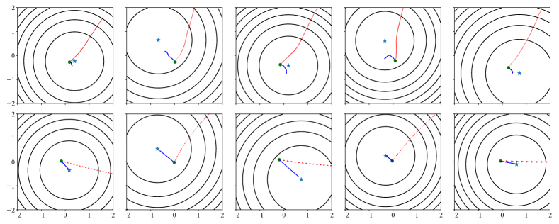
Moreover, under the linearized network, we can conveniently analyze the trajectories of GD and NGD. Notably, we analyze the paths taken by GD and NGD in both output space and weight space. The dynamics with infinitesimal step size are summarized as follow.
| (109) |
By standard matrix differential equation theory, we have
| (110) | ||||
By some manipulations, we can show , which means that gradient descent and natural gradient descent converge to the same point, though these two paths are typically different. Notably, the limiting distance (for both GD and exact NGD) converges to min-norm least squares solution.