Search of QCD phase transition points in the canonical approach of the NJL model

Abstract

We study the Lee-Yang zeros in the canonical approach to search phase transition points at finite temperature and density in the Nambu-Jona-Lasinio (NJL) model as an effective model of QCD. The canonical approach is a promising method to avoid the sign problem in lattice QCD at finite density. We find that a set of Lee-Yang zeros computed with finite degrees of freedom can be extrapolated to those with infinite degrees of freedom, providing the correct phase transition point. We propose the present method as a useful method for actual lattice simulations for QCD.

1 Introduction

The role of Quantum Chromodynamics (QCD), the theory of the strong interaction, at finite temperature and density is increasing as it provides basic inputs in the fundamental questions such as the matter generation in the early universe, formation of galaxies and stars, and mysterious stellar objects such as neutron stars and black-halls. Especially, the latter objects are under active discussions due to the recent observation of gravitational waves [1, 2] and black-halls [3]. Experimentally, those problems are approached by the high energy accelerators at such as J-PARC (KEK/JAEA), FAIR (GSI) and NICA (JINR), which will be expected to operate in the near future. Theoretically, lattice QCD is known as a unique method for the first principle calculations of QCD.

However, lattice QCD suffers from the sign problem at finite density. Many methods have been proposed toward avoiding the sign problem. Meanwhile, a method called the canonical approach [4] has been recently developed rapidly with multiple-precision arithmetic [5, 6, 7, 8, 9, 10, 11, 12, 13, 14, 15, 16, 17, 18]. In the canonical approach physical quantities are calculated at pure imaginary chemical potentials, in which the sign problem does not exist. Information at physical real finite chemical potentials is extracted. The canonical approach can predict physical observable such as particle distributions in heavy ion collisions and reveal the phase structure at high densities.

In Ref. [18], one of the present authors studied the so-called Lee-Yang zeros (LYZs), which are zeros of grand canonical partition functions as functions of the fugacity parameter. LYZs provide us with various information of phase transitions [19, 20]. However, numerical simulations can be only available with finite degrees of freedom, which should be extrapolated to the real situation with infinite degrees of freedom. Currently, such extrapolation method is not known.

To attack this problem, we propose to study in an effective model of QCD, the Nambu-Jona-Lasinio (NJL) model [21, 22]. Because phase properties are known well in the model e.g. [23, 24], we can study exclusively the effect of finite degrees of freedom. We show how the LYZs with finite degrees of freedom are smoothly extrapolated to those with infinite degrees of freedom. Moreover, we also study an additional approximation for the number density as a function of imaginary chemical potential which has been used in the lattice simulations [14, 15, 16, 17, 18]. Taking into account the two features, phase transition points are well determined from the data of finite degrees of freedom.

We will begin, in Sec. 2, by briefly describing the canonical approach in the NJL model. In Sec. 3, we introduce LYZs and a computational method of LYZs. In Sec. 4, the numerical results are shown. After that, we discuss the extrapolation procedure from the analysis of finite degrees of freedom to the case of infinite degrees of freedom. Section 5 is devoted to the summary.

2 Canonical approach in the NJL model

Let us begin with a brief review of the canonical approach. The grand canonical partition function $Z_{GC}$ at a quark chemical potential $\mu$, a temperature $T$ and a volume $V$ of the system can be written as

$$Z_{\rm GC}(\mu,T,V) = \sum_{n=-\infty}^{\infty}\left\langle n\right|e^{-\left(\hat{H}-\mu\hat{N}\right)/T}\left|n\right\rangle$$ (1)

$$= \sum_{n=-\infty}^{\infty}Z_{C}(n,T,V)\xi^{n}\ ,$$

where $\hat{H}$, $\hat{N}$, $\xi$ and $Z_{C}(n,T,V)$ are the Hamiltonian operator, the quark number operator, the quark fugacity defined by $\xi=e^{\mu/T}$ and the canonical partition functions, respectively. Applying Fourier transformation to $Z_{GC}$ at the pure imaginary chemical potential $\mu=i\mu_{I}$ $(\mu_{I}\in\mathbb{R})$, we obtain the canonical partition functions,

$$\!\!\!\!\!\!\!\!Z_{C}(n,T,V) = \int_{0}^{2\pi}\frac{d\theta}{2\pi}\,e^{-in\theta}Z_{\rm GC}(i\mu_{I},T,V)\ ,\ \ \$$ (2)

where $\theta=\frac{\mu_{I}}{T}$. In order to suppress the cancellation of significant digits that comes from the high frequency of $e^{-in\theta}$ at large $n$, we perform Fourier transformation with multiple-precision arithmetic.

In lattice QCD calculations, moreover, the integration method [14, 15, 16, 17, 18] is used to extract $Z_{C}$ for large $n$. In the integration method, $Z_{GC}(i\mu_{I})$ is evaluated from the number density,

$$\frac{n_{q}}{T^{3}}(i\mu_{I}) = \frac{1}{VT^{2}}\frac{\partial}{\partial(i\mu_{I})}\ln Z_{GC}(i\mu_{I})\ .$$ (3)

Since $Z_{GC}(i\mu_{I})$ is a real quantity, we define $n_{q}$ by the real valued $n_{qI}$ by $n_{q}=in_{qI}$ at $\mu=i\mu_{I}$. It is well known that $n_{qI}$ can be approximated by a Fourier series,

$$\frac{n_{qI}}{T^{3}}(\theta) = \sum_{k=1}^{N_{{\sin}}}f_{k}\sin(k\theta)\ ,$$ (4)

with a finite number of terms of $N_{\sin}$ [25, 26]. Fitting the Fourier series to $n_{qI}$, we can evaluate $Z_{GC}$ at the imaginary $\mu$ in good approximation from

$$\!\!\!\!\!\!\!\!\!\!\!\!Z_{\rm GC}(i\mu_{I},T,V) = C\exp{\left\{-V\int^{\theta}_{0}d\theta^{\prime}\,n_{qI}(\theta^{\prime})\right\}}$$ (5)

$$= C\exp{\left\{VT^{3}\sum_{k=1}^{N_{\sin}}\frac{f_{k}}{k}\cos\left(k\theta\right)\right\}}\ ,\ \ \ \ \$$

where $C$ is an integration constant.

In this paper, we compute $n_{qI}$ in Eq. (4) in the NJL model. The Lagrangian density of the NJL model is

$$\!\!\!\!\!\!\!\!\!\!\!\!\!\cal{L} = \bar{\psi}\left(i\gamma^{\nu}\partial_{\nu}-m_{q}\right)\psi+G\left[\left(\bar{\psi}\psi\right)^{2}+\left(\bar{\psi}i\gamma_{5}\vec{\tau}\psi\right)^{2}\right]\,,\ \ \ \$$ (6)

where $\psi$ is the quark field with two flavors ($N_{f}=2$) and three colors ($N_{c}=3$) [23, 24]. Given the current quark mass $m_{q}=5.5$ [MeV], the remaining parameters, the coupling constant $G$ and the cutoff $\Lambda$ are determined such that the pion decay constant $f_{\pi}=93$ [MeV] and the constituent quark mass $m_{q}=335$ [MeV] are reproduced in the mean field approximation, $G=5.5$  [GeV^-2] and $\Lambda=631$ [MeV]. First we investigate the case of infinite volume. In this case, the thermodynamic potential (per unit volume) $\omega$ is defined by utilizing the Matsubara formula as

$$\!\!\!\!\!\!\!\!\!\!\!\!\!\omega(T,\mu)$$ (7)

$$\!\!\!\!\!\!\!\!\!\!\!\!\!\!\!\!\!\!\!\!\!\!=\ \frac{1}{2G}\left(M-m_{q}\right)^{2}$$

$$\!\!\!\!\!\!\!\!\!\!\!\!\!\!\!\!\!\!\!\!\!\!-\ 2N_{c}N_{f}\int\frac{d^{3}p}{\left(2\pi\right)^{3}}\Big{\{}E_{p}+T\ln\left[1+e^{-\left(E_{p}+\mu\right)/T}\right]$$

$$\ \ \ \ \ \ \ \ \ \ \ \ \ \ \ \ \ \ \ \ +T\ln\left[1+e^{-\left(E_{p}-\mu\right)/T}\right]\Big{\}}\,,\ \ \ \$$

where the energy and the constituent quark mass are given as $E_{p}=\sqrt{p^{2}+M^{2}}$ and $M=m_{q}-G\sigma$, respectively. The chiral condensate $\sigma\equiv\langle\bar{\psi}\psi\rangle$ is evaluated from the stationary condition $\partial\omega/\partial\sigma=0$.

Since the number density $n_{q}$ is defined as $n_{q}\equiv-\partial\omega/\partial\mu$, we find in the NJL model

$$\!\!\!\!\!\!\!\!\!\!\!\!\!n_{qI}(\theta) = \frac{1}{G}\frac{\partial M}{\partial\mu_{I}}\left(M-m_{q}\right)$$ (8)

$$- 2N_{c}N_{f}\int\frac{d^{3}p}{\left(2\pi\right)^{3}}\Bigg{\{}\frac{\partial E_{p}}{\partial\mu_{I}}$$

$$-\frac{\partial E_{p}}{\partial\mu_{I}}\frac{2\left(1+e^{E_{p}/T}\cos\theta\right)}{\left(1+e^{E_{p}/T}\cos\theta\right)^{2}+e^{2E_{p}/T}\sin^{2}\theta}$$

$$-\frac{2e^{E_{p}/T}\sin\theta}{\left(1+e^{E_{p}/T}\cos\theta\right)^{2}+e^{2E_{p}/T}\sin^{2}\theta}\Bigg{\}}\,.$$

Note that the constituent quark mass $M$ in Eq. (8) obeys the following gap equation:

$$\!\!\!\!\!\!\!\!\!\!\!\!\!\!\!M\!\!\!\! = \!\!\!\!m_{q}+2N_{c}N_{f}GM$$

$$\times \!\!\!\!\!\!\int\!\!\frac{d^{3}p}{\left(2\pi\right)^{3}}\frac{1}{E_{p}}\Bigg{\{}1-\frac{2\left(1+e^{E_{p}/T}\cos\theta\right)}{\left(1+e^{E_{p}/T}\cos\theta\right)^{2}+e^{2E_{p}/T}\sin^{2}\theta}\Bigg{\}}.\!$$

Table 1: Results for fitting coefficients $f_{k}$ from the data of $n_{qI}/T^{3}$ for each temperature. The values of $f_{k}$ in the list are rounded to three significant digits although errors for all $f_{k}$ are very small, $\delta f_{k}<3\times 10^{-15}$.

$T$ [MeV]	$f_{1}$	$f_{2}$	$f_{3}$	$f_{4}$	$f_{5}$	$f_{6}$	$f_{7}$
29	$6.51\times 10^{-4}$	$1.87\times 10^{-9}$	—	—	—	—	—
39	$8.56\times 10^{-3}$	$6.15\times 10^{-7}$	$6.52\times 10^{-11}$	—	—	—	—
49	$3.69\times 10^{-2}$	$1.81\times 10^{-5}$	$1.31\times 10^{-8}\,\,$	$1.11\times 10^{-11}$	—	—	—
59	$9.31\times 10^{-2}$	$1.63\times 10^{-4}$	$4.24\times 10^{-7}\,\,$	$1.29\times 10^{-9}\,\,$	$4.30\times 10^{-12}$	—	—
79	$2.69\times 10^{-1}$	$2.28\times 10^{-3}$	$2.86\times 10^{-5}\,\,$	$4.19\times 10^{-7}\,\,$	$6.65\times 10^{-9}\,\,$	$1.11\times 10^{-10}$	$1.91\times 10^{-12}$

3 Lee-Yang zeros

In numerical calculations, the fugacity expansion of the grand canonical partition function in Eq. (1) is truncated at a finite value $N_{\rm max}$ as

$$\!\!\!\!\!\!\!Z_{\rm GC}(\mu,T,V) = \sum_{n=-N_{\rm max}}^{N_{\rm max}}Z_{C}(n,T,V)\xi^{n}\ .$$ (10)

Since $N_{\rm max}$ is the maximal value of the net-quark number in the system, degrees of freedom of the system are limited by the finite $N_{\rm max}$. Therefore, we need to take the limit $N_{\rm max}\to\infty$ because a system with a finite degree of freedom does not have a phase transition in the real finite chemical potential.

The theorems of Yang and Lee [19, 20] are of universal and powerful use to investigate phase structures for a system with finite degrees of freedom. The so-called Lee-Yang zeros (LYZs), which are the zeros of grand canonical partition functions in complex fugacity plane, provide us with various information of phase transitions. LYZs are given as roots of the polynomial equation of degree of $2N_{\rm max}$,

$$\xi^{N_{\rm max}}\sum_{n=-N_{\rm max}}^{N_{\rm max}}Z_{C}(n,T,V)\xi^{n} = 0\ ,$$ (11)

in the complex $\xi$ plane. As $N_{\rm max}$ increases, a distribution of LYZs forms one-dimensional curves in the complex $\xi$ plane. If there is a point where LYZs accumulate and are stable as $N_{\rm max}$ increases, the point represents the phase transition point. Therefore, we investigate the $N_{\rm max}$ dependence of distributions of LYZs near the real positive axis of $\xi$.

A polynomial equation of high degree of $2N_{\rm max}$ such as Eq. (11) is known as an ill-posed problem because of significant cancelations. A new method to overcome the difficulty was proposed in Ref. [27]: the cut Baum-Kuchen (cBK) algorithm with multiple-precision arithmetic. In order to solve the equation, we implement the cBK algorithm and a multiple-precision arithmetic package, FMLIB [28].

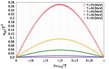
Figure 1: (color online). The $\theta$ dependence of the imaginary number density.

Due to the following properties of $Z_{C}$, it is sufficient to search the LYZs only inside the upper half of the unit circle in the complex $\xi$ plane, (i) $Z_{C}$ satisfy

$$Z_{C}(+n,T,V) = Z_{C}(-n,T,V)\ ,$$ (12)

which comes form the charge-parity invariance of quarks, and (ii) $Z_{C}$ are real. If there is a LYZ at $\xi$, LYZs also exist at $\xi^{-1}$ and $\xi^{\ast}$ because of the properties (i) and (ii), respectively. In this paper, we only show LYZs inside the upper half of the unit circle in the complex $\xi$ plane since whole LYZs can be reconstructed from them.

4 Numerical results

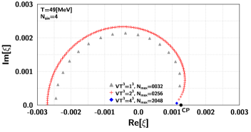
Figure 2: (color online). The $V$ dependence of LYZs in the complex $\xi$ plane. The black filled circle corresponds to the expected critical point (CP) calculated at the real finite chemical potential.

4.1 Imaginary number density

Figure 1 shows the pure imaginary chemical potential dependence of the imaginary number density. We calculate the number density $n_{qI}/T^{3}$ at 161 values of $\mu_{I}$ for various temperature. Since there is an anti-symmetry, $n_{qI}(\pi+\theta)=-n_{qI}(\pi-\theta)$, the figure only shows the region $0\leq\theta\leq\pi$. Because the critical point in the NJL model is already known as $(T_{\rm CP},\mu_{\rm CP})\simeq(49,327)$ [MeV], we choose the temperatures at $T_{\rm CP}$ (49 [MeV]), below $T_{\rm CP}$ (29 and 39 [MeV]) and above $T_{\rm CP}$ (59 and 79 [MeV]). It turns out that $n_{qI}$ is well fitted by the Fourier series of Eq. (4) with the coefficients $f_{k}$ as listed in Table 1.

4.2 Distributions of LYZs

We calculate the canonical partition functions from the imaginary number density by performing Fourier transforms in Eq. (2) with 5,000 significant digits in decimal notation. After the cBK algorithm is carried out with 300 significant digits, we obtain LYZs. Because, in the cBK algorithm, coordinates of LYZs are identified with finite sizes of the annulus sectors, LYZs have the systematic errors of the cBK algorithm: $\delta|\xi|/|\xi|<1.6\times 10^{-2}$ and $\delta\left({\rm arg}\left(\xi\right)\right)/{\rm arg}\left(\xi\right)<6.5\times 10^{-2}$ for all LYZs. The systematic errors are tiny compared to values of LYZs. Therefore, the systematic errors are not displayed in the following figures.

In Fig. 2, we present the distributions of LYZs. LYZs form an one-dimensional curve like a circle in the complex $\xi$ plane. The black filled point labeled by CP corresponds to the expected critical point evaluated from calculations at real chemical potential.

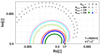
Figure 3: (color online). The $N_{\rm max}$ and $N_{\sin}$ dependences of LYZs in the complex $\xi$ plane. The black filled circle corresponds to the expected critical point (CP) calculated at the real finite chemical potential.

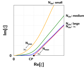
Figure 4: (color online). Schematic flows of the right edges of LYZs as $N_{\rm max}$ and $N_{\sin}$ are varied.

We also show the volume dependence of LYZs in Fig. 2. The imaginary number density in Fig. 1 is calculated in the NJL model with infinite volume. However, the finite volume effect of the system appears from Eq. (5) in the canonical approach. Following Refs. [27, 18], we choose $N_{\rm max}$ so that the value of $N_{\rm max}/V$ is approximately unchanged when $V$ changes. Figure 2 indicates that the right edges of LYZs, which is defined by a position of $\min[{\rm Im}(\xi)]$ in the first quadrant in the complex $\xi$ plane, approach the expected CP as $V$ increases. Note that we only calculate the right edge of LYZs for $VT^{3}=4^{3}$ due to a large computational time in the cBK algorithm. Because the right edges of LYZs are close to the expected CP at $VT^{3}\geq 2^{3}$, we can safely discuss extraction of the expected CP from LYZs at $VT^{3}=2^{3}$.

4.3 $N_{\rm max}$ and $N_{\sin}$ dependences and fitting curves

In the canonical approach, there are two parameters, $N_{\rm max}$ and $N_{\sin}$. In Fig. 3, we show how the right edge depends on these parameters. We find that for finite $N_{\sin}$ as $N_{\rm max}$ increases, the right edges of LYZs pass over the expected CP and go to the origin. The behavior is more noticeable for smaller $N_{\sin}$. The reason why the right edges do not approach the CP but do the origin in large-$N_{\rm max}$ limit is that the imaginary number density is approximated by a Fourier series with finite terms as in Eq. (4). In this case, phase transitions do not occur in the real chemical potential. Schematic flows of the right edges of LYZs against $N_{\rm max}$ and $N_{\sin}$ changes are summarized in Fig. 4.

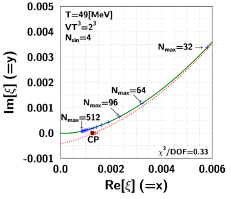
Figure 5: (color online). The $N_{\rm max}$ dependence of LYZs at $T=49$ [MeV] in the complex $\xi$ plane. The blue crosses stand for the right edges of LYZs. The solid and dotted curves represent the fitting function of the right edges of LYZs and the curve subtracting the first term from the fitting function. The red open circle means a point, $\xi=(x_{0},0)$, where is the intersection of the dotted curve and the real axis. The black filled circle corresponds to the expected critical point (CP) calculated at the real finite chemical potential.

To obtain more insight on the results and to extract the phase transition point by the data with finite $N_{\rm max}$ and $N_{\sin}$, we try to fit the right edges of LYZs by a trial function. Figure 5 shows the $N_{\rm max}$ dependence of the right edges of LYZs. The points are computed at $N_{\rm max}=32\mathchar 45\relax$512 by a step 32 as shown there. We chose a fitting function as

$$\!\!\!\!\!\!\!y = \frac{b\left(cx_{0}-dx_{0}^{2}\right)}{x+b}+c\left(x-x_{0}\right)+d\left(x-x_{0}\right)^{2}\ ,\ \ \ \ \$$ (13)

where $y={\rm Im}[\xi]$, $x={\rm Re}[\xi]$ with the parameters $b$, $c$, $d$ and $x_{0}$. This functional form is inspired by the expected behavior in the presence of the phase transition satisfying $y(x_{0})=0$ in the limit $N_{\rm max},N_{\sin}\to\infty$. This is implemented by the polynomial term which is nothing but the Taylor expansion at $x_{0}$, and hence $y(x_{0})=0$ is automatically satisfied. In contrast, for finite $N_{\sin}$, $y$ deviates from that and should approach the origin in the limit $N_{\rm max}\to\infty$. Indeed by adding the first term the trial functions satisfies $y(0)=0$. In the absence of the phase transition, this argument can not be applied but is replaced by an instability of the fitting as we will discuss shortly.

In Fig. 5, the right edges of LYZs computed at $N_{\sin}=4$ and at various $N_{\rm max}$ from 32 to 512 with a step 32 are shown by blue cross points. The green solid line is the fitted function by Eq. (13) and the red dotted line the one of the polynomial term. The fitting is performed by the weighted least-squares method where the weights $1/(\delta y_{i})^{2}$ are given by the systematic errors of the cBK algorithm $\delta y_{i}$. We find that the data points of the right edges of the LYZs are reproduced with good accuracy: $\chi^{2}/{\rm DOF}=3.95/12$. As if to prove that the first term is the finite $N_{\sin}$ effect, the curve subtracting the first term, which is represented by the dotted curve, crosses the real axis at $x_{0}=1.33(14)\times 10^{-3}$. The result is consistent with the value of expected CP, $\xi_{\rm CP}=1.26\times 10^{-3}$. Note that the other parameters $c$ and $d$ in the resulting curve are also the same as the ones of the fitting function: $c=4.15(34)\times 10^{-1}$ and $d=7.26(15)\times 10$.

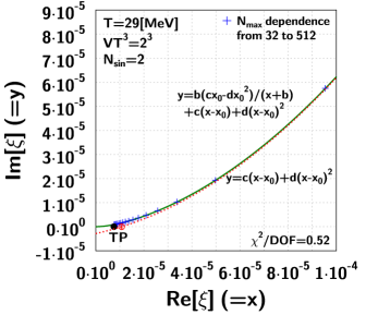
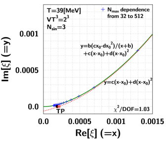
Figure 6: (color online). The $N_{\rm max}$ dependence of LYZs at $T=29$ and 39 [MeV] in the complex $\xi$ plane. The blue crosses stand for the right edges of LYZs. The black filled circle corresponds to the expected transition point (TP) calculated at the real finite chemical potential.

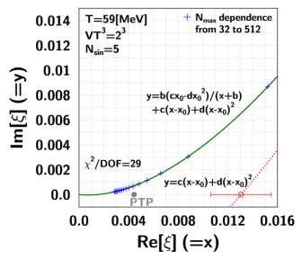
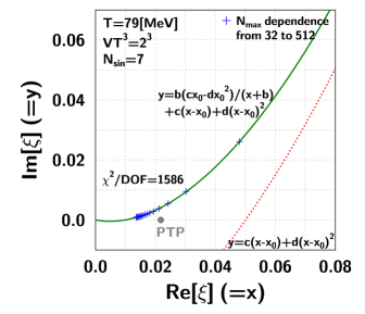
Figure 7: (color online). The $N_{\rm max}$ dependence of LYZs at $T=59$ and 79 [MeV] in the complex $\xi$ plane. The blue crosses stand for the right edges of LYZs. The gray filled circle corresponds to the expected pseudo transition point (PTP) calculated at the real finite chemical potential. In the right figure ($T=79$ [MeV]), the intersection of the dotted curve and the real axis is not represented because the intersection has a large error, $x_{0}=0.050(137)$.

In Fig. 6, we also show the $N_{\rm max}$ dependence of LYZs at low temperatures, 29 and 39 [MeV]. Then, we find that the extrapolation procedure performed in the simulation at $T=49$ [MeV] works well to obtain the expected transition points (TP) with good accuracy. Therefore, we can conclude that the extrapolation procedure of LYZs is reasonable to extract the correct transition points from the canonical approach.

Finally, Figure 7 shows the $N_{\rm max}$ dependence at high temperatures, 59 and 79 [MeV] where there is no phase transition. It is interesting to see how the extrapolation procedure works in this case. From values of $\chi^{2}/{\rm DOF}=29$ ($T=59$ [MeV]) and 1586 ($T=79$ [MeV]), we find that the fits of the LYZs become unstable at high temperatures. In Fig. 7 we also show the peaks of susceptibility of the number density at the crossover represented as the pseudo transition points (PTP). Our results obtained from the extrapolation procedure are far from the PTP, which is consistent with the disappearance of phase transition points. The results indicate that the stability of the fit of the right edges of LYZs distinguishes between regions with and without phase transition points.

5 Summary

We have investigated phase transition points from LYZs calculated in the canonical approach of the two-flavor NJL model. After we have extracted the canonical partition functions from the imaginary number density by using the integration method and multiple-precision arithmetic, the LYZs have been evaluated with the cBK algorithm. In the integration method, we have fitted a Fourier series to the 161 data of the number densities as functions of imaginary chemical potential. Because phase transition structures of the NJL model are already known with the critical point, $(T_{\rm CP},\mu_{\rm CP})\simeq(49,327)$ [MeV], simulations have been carried out at several temperatures around $T_{\rm CP}$, $T=29$, 39, 49, 59 and 79 [MeV].

We have shown how the LYZs behave as functions of the volume of the system $V$, $N_{\sin}$ and $N_{\rm max}$. The results of the $V$ dependence at $T=49$ [MeV] have shown that the simulation $VT^{3}=2^{3}$ has a sufficiently large $V$.

In the investigation of the $N_{\rm max}$ dependence of LYZs, we have extrapolated the right edges of LYZs from finite $N_{\rm max}$ to the infinite $N_{\rm max}$. We have succeeded in subtracting a term associated with an artifact due to finite $N_{\sin}$ from the fitted function at $T\leq T_{\rm CP}$. We have found that the curve with the finite $N_{\sin}$ effect subtracted crosses the real axis of $\xi$ near the expected transition point calculated at the real finite chemical potential. The extrapolation procedure becomes unstable at $T>T_{\rm CP}$, which is consistent with the lack of phase transition points at the real chemical potential. The results indicate that the accuracy of the fitting of the right edges of LYZs distinguishes between regions with and without phase transition points.

In this paper, we have discussed LYZs of the NJL model and have found a reasonable extrapolation procedure. Whether the extrapolation procedure has universality for models or not is open to discussion.

References

- [1] B. P. Abbott et al. [LIGO Scientific and Virgo Collaborations], “Observation of Gravitational Waves from a Binary Black Hole Merger,” Phys. Rev. Lett. 116, no. 6, 061102 (2016) [arXiv:1602.03837 [gr-qc]].
- [2] B. P. Abbott et al. [LIGO Scientific and Virgo Collaborations], “GW170817: Observation of Gravitational Waves from a Binary Neutron Star Inspiral,” Phys. Rev. Lett. 119, no. 16, 161101 (2017) [arXiv:1710.05832 [gr-qc]].
- [3] K. Akiyama et al. [Event Horizon Telescope Collaboration], “First M87 Event Horizon Telescope Results. VI. The Shadow and Mass of the Central Black Hole,” Astrophys. J. 875, no. 1, L6 (2019).
- [4] A. Hasenfratz and D. Toussaint, “Canonical ensembles and nonzero density quantum chromodynamics,” Nucl. Phys. B 371, 539 (1992).
- [5] K. Morita, V. Skokov, B. Friman and K. Redlich, “Net baryon number probability distribution near the chiral phase transition,” Eur. Phys. J. C 74, 2706 (2014) [arXiv:1211.4703 [hep-ph]].
- [6] R. Fukuda, A. Nakamura and S. Oka, “Canonical approach to finite density QCD with multiple precision computation,” Phys. Rev. D 93, no. 9, 094508 (2016) [arXiv:1504.06351 [hep-lat]].
- [7] A. Nakamura, S. Oka and Y. Taniguchi, “QCD phase transition at real chemical potential with canonical approach,” JHEP 1602, 054 (2016) [arXiv:1504.04471 [hep-lat]].
- [8] P. de Forcrand and S. Kratochvila, “Finite density QCD with a canonical approach,” Nucl. Phys. Proc. Suppl. 153, 62 (2006) [hep-lat/0602024].
- [9] S. Ejiri, “Canonical partition function and finite density phase transition in lattice QCD,” Phys. Rev. D 78, 074507 (2008) [arXiv:0804.3227 [hep-lat]].
- [10] A. Li, A. Alexandru, K. F. Liu and X. Meng, “Finite density phase transition of QCD with and using canonical ensemble method,” Phys. Rev. D 82, 054502 (2010) [arXiv:1005.4158 [hep-lat]].
- [11] A. Li, A. Alexandru and K. F. Liu, “Critical point of QCD from lattice simulations in the canonical ensemble,” Phys. Rev. D 84, 071503 (2011) [arXiv:1103.3045 [hep-ph]].
- [12] J. Danzer and C. Gattringer, “Properties of canonical determinants and a test of fugacity expansion for finite density lattice QCD with Wilson fermions,” Phys. Rev. D 86, 014502 (2012) [arXiv:1204.1020 [hep-lat]].
- [13] C. Gattringer and H. P. Schadler, “Generalized quark number susceptibilities from fugacity expansion at finite chemical potential for = 2 Wilson fermions,” Phys. Rev. D 91, no. 7, 074511 (2015) [arXiv:1411.5133 [hep-lat]].
- [14] D. L. Boyda, V. G. Bornyakov, V. A. Goy, V. I. Zakharov, A. V. Molochkov, A. Nakamura and A. A. Nikolaev, “Novel approach to deriving the canonical generating functional in lattice QCD at a finite chemical potential,” JETP Lett. 104, no. 10, 657 (2016) [Pisma Zh. Eksp. Teor. Fiz. 104, no. 10, 673 (2016)].
- [15] V. A. Goy, V. Bornyakov, D. Boyda, A. Molochkov, A. Nakamura, A. Nikolaev and V. Zakharov, “Sign problem in finite density lattice QCD,” PTEP 2017, no. 3, 031D01 (2017) [arXiv:1611.08093 [hep-lat]].
- [16] V. G. Bornyakov, D. L. Boyda, V. A. Goy, A. V. Molochkov, A. Nakamura, A. A. Nikolaev and V. I. Zakharov, “New approach to canonical partition functions computation in lattice QCD at finite baryon density,” Phys. Rev. D 95, no. 9, 094506 (2017) [arXiv:1611.04229 [hep-lat]].
- [17] D. Boyda, V. G. Bornyakov, V. Goy, A. Molochkov, A. Nakamura, A. Nikolaev and V. I. Zakharov, “Lattice Study of QCD Phase Structure by Canonical Approach - Towards determining the phase transition line,” arXiv:1704.03980 [hep-lat].
- [18] M. Wakayama, V. G. Borynakov, D. L. Boyda, V. A. Goy, H. Iida, A. V. Molochkov, A. Nakamura and V. I. Zakharov, “Lee-Yang zeros in lattice QCD for searching phase transition points,” Phys. Lett. B 793, 227 (2019) [arXiv:1802.02014 [hep-lat]].
- [19] C. N. Yang and T. D. Lee, “Statistical theory of equations of state and phase transitions. 1. Theory of condensation,” Phys. Rev. 87, 404 (1952).
- [20] T. D. Lee and C. N. Yang, “Statistical theory of equations of state and phase transitions. 2. Lattice gas and Ising model,” Phys. Rev. 87, 410 (1952).
- [21] Y. Nambu and G. Jona-Lasinio, “Dynamical Model of Elementary Particles Based on an Analogy with Superconductivity. 1.,” Phys. Rev. 122, 345 (1961). doi:10.1103/PhysRev.122.345
- [22] Y. Nambu and G. Jona-Lasinio, “Dynamical Model Of Elementary Particles Based On An Analogy With Superconductivity. Ii,” Phys. Rev. 124, 246 (1961). doi:10.1103/PhysRev.124.246
- [23] T. Kunihiro, “Quark number susceptibility and fluctuations in the vector channel at high temperatures,” Phys. Lett. B 271, 395 (1991). doi:10.1016/0370-2693(91)90107-2
- [24] T. Hatsuda and T. Kunihiro, “QCD phenomenology based on a chiral effective Lagrangian,” Phys. Rept. 247, 221 (1994) doi:10.1016/0370-1573(94)90022-1 [hep-ph/9401310].
- [25] M. D’Elia and F. Sanfilippo, “Thermodynamics of two flavor QCD from imaginary chemical potentials,” Phys. Rev. D 80, 014502 (2009) [arXiv:0904.1400 [hep-lat]].
- [26] T. Takaishi, P. de Forcrand and A. Nakamura, “Equation of State at Finite Density from Imaginary Chemical Potential,” PoS LAT 2009, 198 (2009) [arXiv:1002.0890 [hep-lat]].
- [27] A. Nakamura and K. Nagata, “Probing QCD phase structure using baryon multiplicity distribution,” PTEP 2016, no. 3, 033D01 (2016) [arXiv:1305.0760 [hep-ph]].
- [28] D. M. Smith, Multiple Precision Computation, FMLIB1.3 (2015). http://myweb.lmu.edu/dmsmith/FMLIB.html.