Incremental Learning Using a Grow-and-Prune Paradigm with Efficient Neural Networks

Abstract

Deep neural networks (DNNs) have become a widely deployed model for numerous machine learning applications. However, their fixed architecture, substantial training cost, and significant model redundancy make it difficult to efficiently update them to accommodate previously unseen data. To solve these problems, we propose an incremental learning framework based on a grow-and-prune neural network synthesis paradigm. When new data arrive, the neural network first grows new connections based on the gradients to increase the network capacity to accommodate new data. Then, the framework iteratively prunes away connections based on the magnitude of weights to enhance network compactness, and hence recover efficiency. Finally, the model rests at a lightweight DNN that is both ready for inference and suitable for future grow-and-prune updates. The proposed framework improves accuracy, shrinks network size, and significantly reduces the additional training cost for incoming data compared to conventional approaches, such as training from scratch and network fine-tuning. For the LeNet-300-100 and LeNet-5 neural network architectures derived for the MNIST dataset, the framework reduces training cost by up to 64% (63%) and 67% (63%) compared to training from scratch (network fine-tuning), respectively. For the ResNet-18 architecture derived for the ImageNet dataset and DeepSpeech2 for the AN4 dataset, the corresponding training cost reductions against training from scratch (network fine-tunning) are 64% (60%) and 67% (62%), respectively. Our derived models contain fewer network parameters but achieve higher accuracy relative to conventional baselines.

1 Introduction

In recent years, deep neural networks (DNNs) have achieved remarkable success and emerged as an extraordinarily powerful tool for a wide range of machine learning applications. Their ability to represent input data through increasingly more abstract layers of feature representations and knowledge distillation has been shown to be extremely effective in numerous application areas, such as image recognition, speech recognition, disease diagnosis, and neural machine translation [1, 2, 3, 4, 5, 6]. With increased access to large amounts of labeled training data (e.g., ImageNet [7] with 1.2 million training images from 1,000 different categories) and computational resources, DNNs have resulted in human-like or even super-human performance on a variety of tasks.

A typical development process of a DNN starts with training a model based on the target dataset that contains a large amount of labeled training instances. The DNN learns to distill intelligence and extract features from the dataset in this process. The well-trained model is then used to make predictions for incoming unseen data [8]. In such a setting, all the labeled data are presented to the network all-at-once for one training session. While effective, this may be too idealized for many real-world scenarios where training data and their associated labels may be collected in a continuous and incremental manner, and only some data instances may be used initially to obtain the first trained model. For example, biomedical datasets are typically updated regularly when the number of data points obtained from patients increases, or disease trends shift across time [9]. This makes it necessary to update a DNN model frequently to accommodate the new data and capture the new information effectively.

A widely-used approach for updating DNNs to learn new information involves discarding the existing model and retraining the DNN weights from scratch using all the data acquired so far [10, 8]. This method leads to a complete loss of all the previously accumulated knowledge in the pre-trained network, and suffers from three major problems:

• Vast training cost: Training from scratch at each update is computationally- and time-intensive. Ideally, an incremental learning system should combine existing knowledge with new knowledge in a continuous and efficient manner, hence minimizing additional computational costs of an update.

• Fixed network capacity: Conventional DNN models have fixed and static architectures. As new data become available, it is not possible to increase their capacity during the entire training process.

• Massive redundancy: The generated DNN models derived for large real-world datasets are typically over-parameterized [11] and can easily contain millions of parameters, as shown in Table I. Such a large model size incurs substantial storage and memory cost during inference.

TABLE I: Model size of DNNs for real-world applications

Network	Task	#Parameters
AlexNet [1]	Image classification	61M
VGG-16 [12]	Image classification	138M
ResNet-18[13]	Image classification	12M
ResNet-152 [13]	Image classification	60M
DeepSpeech2 [14]	Speech recognition	50M
Seq2Seq [5]	Machine translation	384M

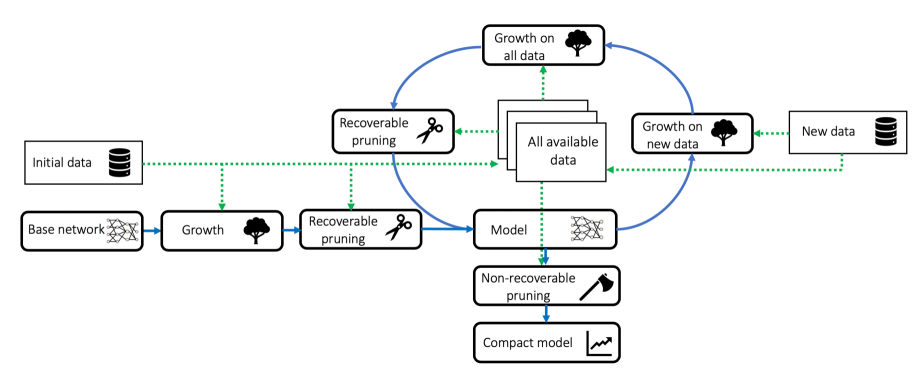
Figure 1: Flowchart of the proposed incremental framework.

To address the above problems, we propose an incremental learning framework based on a grow-and-prune neural network synthesis paradigm. It consists of two sequential training stages in a model update process: gradient-based growth and magnitude-based pruning. We depict the flowchart of the framework in Fig. 1, where the green dashed and blue solid lines depict the data flow path and model update process, respectively. We first grow and prune a model with the initial data. When new data arrive, the network undergoes a growth phase (first, based on new data and then on all available data) that increases its size to accommodate new data and knowledge. Then, we employ a pruning phase to remove redundant parameters to obtain a compact inference model. In this stage, we first use a concept called recoverable pruning to acquire a compact model that is subjected to the next grow-and-prune update, and then use non-recoverable pruning to achieve ultra compactness if the use scenario imposes a very strict resource constraint. We validate our approach across different DNN architectures, datasets, and learning tasks, including LeNets on the MNIST dataset, ResNet-18 on the ImageNet dataset, and DeepSpeech2 on the AN4 dataset. Our incremental learning framework consistently leads to improved accuracy, faster model training, and more compact final inference models relative to conventional approaches, such as training from scratch (TFS) and network fine-tuning (NFT).

The rest of this paper is organized as follows. We review related work in Section 2. In Section 3, we introduce background material that describes the scope and goal of incremental learning as well as hidden-layer long short-term memory (H-LSTM) [15] cells that we use in our experiments. Then, we discuss our proposed incremental learning methodology in detail in Section 4. In Section 5, we present experimental results for both image classification and speech recognition tasks. In Section 6, we discuss the inspirations of our proposed framework from the human brain. Finally, we draw conclusions in Section 7.

2 Related work

Various methods and algorithms have been proposed in the past to design DNN-based incremental learning frameworks and execution-efficient DNNs. We discuss these approaches next.

2.1 Incremental learning

The world of digitized data generates new information at each moment, thus fueling the need for machine learning models that can learn as the new data arrive. We summarize such techniques next.

Transfer learning based approaches: Transfer learning provides a promising solution to the problem of efficient incremental learning with DNNs. It effectively conserves existing knowledge by maintaining the weights and connections of the first several convolutional layers, which are known to be generic feature extractors [16]. For example, Li et al. propose a framework called ‘Learning without Forgeting’ to train the transferred network with only new data while achieving performance improvements. This also obviates the need to learn from scratch for new tasks [17]. Yan et al. exploit common feature sharing in a hierarchical convolutional neural network (CNN) model to achieve better performance compared to their NFT baseline [18]. Another promising approach to efficient incremental learning is to transfer knowledge from a small network to a large one. This yields significant training cost reduction and accuracy gain, as shown by Chen et al. [19].

Architectural evolution approaches: Another way to accommodate new data is to adaptively evolve the network architecture and update the weights simultaneously. Xiao et al. propose an incremental training algorithm that grows a tree-structured network hierarchically [20]. Roy et al. also utilize such tree-structured networks to reduce the training cost by 20% [21]. Alternative methods focus on adding new layers or new nodes to increase network capacity. For instance, Rusu et al. suggest that a progressive neural network can learn to solve complex sequences of tasks by adding additional layers and leveraging prior knowledge with lateral connections [22]. Terekhov et al. also propose an algorithm to reuse existing network capacity and add new blocks of neurons, where the generated model outperforms the baseline network that is trained from scratch [23].

2.2 Efficient and compact neural networks

Most DNNs are computationally intensive and over-parameterized [11]. Several different approaches have been put forward in the literature to design efficient DNNs. These approaches include designing novel compact neural network architectures and compressing existing models. We summarize them next.

Compact architecture design: Exploiting efficient building blocks and operations can significantly cut down on the DNN computation cost. For example, MobileNetV2 effectively shrinks the model size and cuts down the number of floating-point operations (FLOPs) with inverted residual building blocks [24]. Ma et al. propose another compact CNN architecture that utilizes channel shuffle operation and depth-wise convolution [25]. Wu et al. suggest replacing spatial convolution layers with shift-based modules that have zero FLOPs. The generated ShiftNet has substantially reduced computation and storage costs [26]. Besides, automated compact architecture design also provides a promising solution [27]. Dai et al. develop an automated architecture adaptation and search framework based on efficient performance predictors [28]. The searched models deliver up to 8.5% absolute top-1 accuracy gain on the ImageNet dataset compared to MobileNetV2 while reducing latency.

Model compression: Apart from compact architecture design, compressing and simplifying existing models have also emerged as a promising approach [29]. By removing redundant connections and neurons, network pruning has been shown to be very successful at DNN compression. For instance, Han et al. have shown that more than 92% of the connections in VGG-16 can be pruned away without any accuracy loss [11]. A recent work combines pruning with network growth and improves the compression ratio of VGG-16 by another 2.5$\times$ [30]. Furthermore, structured sparsity and pruning can reduce the run-time latency significantly [31]. For example, Yin et al. achieve $2.4\times$ latency reduction for speech recognition on an Nvidia GPU based on hardware-aware structured column and row sparsity [32]. Besides, low-bit quantization is another powerful tool for reducing the storage cost [33]. For instance, Zhu et al. show that replacing a full-precision (32-bit) weight representation with ternary weight quantization only incurs a minor accuracy loss for ResNet-18, but significantly reduces the storage and memory costs [34].

3 Background

In this section, we discuss background material on the scope and goal of incremental learning and H-LSTMs that were used in some of the experiments.

3.1 Scope and aim of incremental learning

Incremental learning refers to the process of learning when input data gradually become available [35]. The goal of incremental learning is to let the machine learning model preserve existing knowledge and adapt to new data at the same time. However, aiming to achieve these two goals simultaneously suffers from the well-known stability-plasticity dilemma [36]: a purely stable model is able to conserve all prior knowledge, but cannot accommodate any new data or information, whereas a completely plastic model has the opposite problem.

Ideally, an incremental learning framework should have the following characteristics [10]:

• Flexible capacity: It should be able to dynamically adjust the model’s learning capability to accommodate newly available data and information.

• Efficient update: Updating the model when new data become available should be efficient and incur only minimal overhead.

• Preserving knowledge: It should maintain existing knowledge in the update process, and avoid restarting training from scratch.

In this work, we introduce another design aim for DNN-based incremental learning systems:

• Compact inference model: It is beneficial to generate a lightweight DNN model for efficient inference.

We will show later how our framework addresses the stability-plasticity dilemma and satisfies all the above requirements.

3.2 Hidden-layer LSTM

As mentioned earlier, we use the H-LSTM concept proposed in [15] in our experiments for time-series data analysis. An H-LSTM is an LSTM variant with improved performance and efficiency. It introduces multi-level abstraction in the control gates of conventional LSTMs that utilize multi-layer perceptron (MLP) neural networks, as shown in Fig. 2, where $\textbf{c}_{t-1}$ and $\textbf{h}_{t-1}$ refer to the cell state tensor and hidden state tensor, respectively, at step $t-1$; $\textbf{x}_{t}$, $\textbf{h}_{t}$, $\textbf{c}_{t}$, $\textbf{f}_{t}$, $\textbf{i}_{t}$, $\textbf{o}_{t}$, and $\textbf{g}_{t}$, refer to the input tensor, hidden state tensor, cell state tensor, forget gate, input gate, output gate, and tensor for cell updates at step $t$, respectively; and $\otimes$ and $\oplus$ refer to the element-wise multiplication operator and element-wise addition operator, respectively.

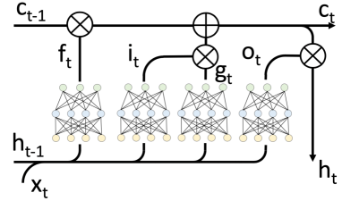
Figure 2: Schematic diagram of an H-LSTM cell. MLP neural networks are used in the control gates.

The MLP gates in an H-LSTM enhance gate control and increase the learning capability of the cell. Moreover, they enable drop-out to be used to optimize the control gates and thus alleviate the regularization difficulty problem faced by conventional LSTM cells [15]. As a result, an H-LSTM based recurrent neural network (RNN) achieves higher accuracy with much fewer parameters and lower run-time latency compared to an LSTM based RNN for many applications, e.g., image captioning and speech recognition.

4 Methodology

In this section, we discuss our proposed incremental learning framework in detail. We first give a high-level overview of the framework, and then detailed descriptions of the specific growth and pruning algorithms.

4.1 Incremental learning framework

As mentioned earlier, the proposed framework is based on a grow-and-prune paradigm, which enables the model to dynamically and adaptively adjust its architecture to accommodate new data and information. We illustrate the growth and pruning process in Fig. 3, where the double and single dashed lines refer to the newly grown and pruned connections, respectively. The initial network inherits the architecture and weights from the model derived in the last update (or uses random weight initialization when starting from scratch for the first model). In the model update process, our framework utilizes two sequential steps to update the DNN model: gradient-based growth and magnitude-based pruning. The network gradually grows new connections based on the gradient information (extracted using the back-propagation algorithm) obtained in the growth phase. Then, it iteratively removes redundant connections based on their magnitudes in the pruning phase. Finally, it rests at a compact and accurate inference model that is ready for deployment and the next update.

Next, we explain the gradient-based growth and magnitude-based pruning procedures in detail.

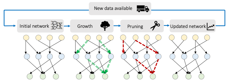
Figure 3: Illustration of the grow-and-prune paradigm in the proposed incremental learning framework.

4.2 Growth phase

4.2.1 Gradient-based growth policy

When new data become available, we use a gradient-base growth approach to adaptively increase the network capacity in order to accommodate new knowledge. The pre-growth network is typically a sparse and partially-connected DNN. In our current implementation, we use a mask tensor Msk to disregard the ‘dangling’ connections (connections that are not used in the network) for each weight tensor W. Msk tensors only have binary values (0 or 1) and have the same size as their corresponding W tensor.

We employ three sequential steps to grow new connections:

• Gradient evaluation: We first evaluate the gradient for all the ‘dangling’ connections. In the network training process, we extract the gradient of all weights ($\textbf{W}.grad$) for each mini-batch of training data with the back-propagation algorithm. We repeat this process and accumulate $\textbf{W}.grad$ over a whole training epoch. Then, we calculate the average gradients over the entire epoch. Note that we pause the parameter update in the gradient evaluation procedure.

• Connection growth: We activate the connections with large gradients. Specifically, we activate a connection $w$ by manually setting the value of its corresponding mask to be 1 if and only if the following condition is met:

  $$|w.grad|\geq\alpha^{th}\text{percentile of}\ \ |\textbf{W}.grad|$$ (1)

  where $\alpha$ is a pre-defined parameter. We typically use $30\leq\alpha\leq 50$ in our experiments. This policy helps us activate connections that are the most efficient at reducing the loss function $L$. This is because connections with large gradients also have large derivatives of $L$:

  $$w.grad=\frac{\partial L}{\partial w}$$ (2)

• Weight initialization: We initialize the weights of newly added connections to $\eta\times w.grad$, where $\eta$ is the current learning rate for training.

Connection growth and parameter training are interleaved in the growth phase, where we periodically conduct connection growth during training. We employ stochastic gradient descent in both the architecture space and parameter space in this process.

The connection growth policy effectively adapts the model architecture to accommodate newly available data and information. To illustrate this, we extract and plot the total number of connections from each input image pixel to the first hidden layer of the post-growth LeNet-300-100 [37] (for the MNIST dataset, in which the images are hand-written digits of size 28$\times$ 28) in Fig. 4. The initial model [Fig. 4(a)] is trained with data that has the label ‘1’ or ‘2’, and thus the connection density distribution is similar to an overlap of digits ‘1’ and ‘2’. Then, we add an additional class with labels ‘0’, ‘6’, and ‘7’, and plot the corresponding connection density distribution of the post-growth network in Fig. 4(b), (c), and (d), respectively. We observe that the network architecture evolves to adapt to the new class of data.

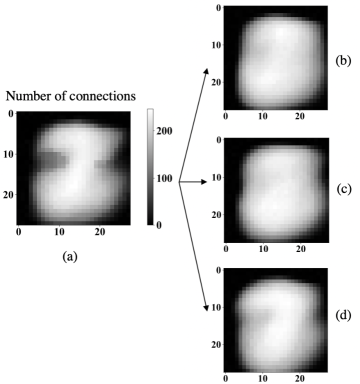
Figure 4: Illustration of the grown connections from the input layer to the first hidden layer of LeNet-300-100 with different training data added.

4.2.2 Growth on new data

To reduce the training cost of a model update, we introduce a mechanism to speed up the growth phase. Specifically, we first employ connection growth and parameter training only on the previously unseen data for a pre-defined number of epochs whenever new data become available. Then, we merge the new data with all the previously available training data, and perform growth and training on all existing data.

This ‘new data first’ policy enables a rapid learning process and architecture update on the new data and significantly reduces overall training cost in the growth phase. We compare the number of training epochs for LeNet-300-100 in Table II using two different approaches:

• Merged training: Merge the new data and existing data, and conduct connection growth and parameter training on all data.

• New data first: Perform growth and training on new data first, then combine the new data and existing data, and finally grow and train on all available data.

In Table II, the initial model is trained on 90% of the MNIST training data. New data and all data refer to the remaining 10% of training data and the entire MNIST training set, respectively. To reach the same target accuracy of 98.67%, our proposed method only requires 15 and 20 training epochs first on new data and then on all data, respectively. Since the number of training instances in new data is 10$\times$ smaller than in all data, the cost of 15 training epochs on new data is equivalent to only 1.5 epochs of training on all data. Thus, the training cost of our proposed approach (15 epochs on new data plus 20 epochs on all data) is equivalent to 21.5 epochs of training on all data. As a result, our proposed method reduces the growth phase training cost by 2.3$\times$ compared to merged training, which requires 49 epochs of training on all data.

TABLE II: Training cost comparison between merged training and ‘new data first’ approaches

Approach	#Training epochs		Accuracy
	New data1	All data
Merged training	-	49	98.67%
New data first (ours)	15	20	98.67%
1: The size of new data is 10$\times$ smaller than the size of all data.

4.3 Pruning phase

We discuss the pruning approach next.

4.3.1 Magnitude-based pruning policy

DNNs are typically very over-parameterized. Pruning has been shown to be very effective in removing redundancy [11]. Thus, we prune away redundant connections for compactness and to ensure efficient inference after the growth phase.

The pruning policy removes weights based on their magnitudes. In the pruning process, we remove a connection $w$ by setting its value as well as the value of its corresponding mask to 0 if and only if the following condition is satisfied:

$$|w|\leq\beta^{th}\text{percentile of}\ \ |\textbf{W}|$$ (3)

where $\beta$ is a pre-defined pruning ratio. Typically, we use $3\leq\beta\leq 5$ in our experiments. Note that connection pruning is an iterative process. In each iteration, we prune the weights that have the smallest values (e.g., smallest 5%), and retrain the network to recover its accuracy. Once the desired accuracy is achieved, we start the next pruning iteration.

4.3.2 Recoverable and non-recoverable pruning

It is important for the incremental learning framework to be sustainable and support long-term learning. This is because we need to update the model frequently for a long period of time in many real-world scenarios. In such settings, the growth and pruning process needs to be executed over numerous cycles. To support long-term learning, the gradient-based growth phase should be able to fully recover the network capacity, architecture, and accuracy from the last post-pruning model. To achieve this, we employ recoverable pruning in the main grow-and-prune based model update process. We explain the recoverable pruning policy next.

We define a pruning process to be recoverable if and only if both of the following conditions are satisfied:

• No neuron pruning: Each neuron in the post-pruning network has at least one input connection and one output connection. This ensures gradient flow in the growth phase in the next update.

• No accuracy loss: The post-pruning model has the same or higher accuracy than the pre-pruning model. This prevents information loss in the pruning phase.

In addition, we use a leaky rectified linear unit (ReLU) with a reverse slope of 0.01 as the activation function $f$ in the entire model update process:

$$f(x)=max(0.01x,x)$$ (4)

This prevents the ‘dying’ neuron problem (a ReLU with constant 0 output has no back-propagated gradient). It keeps all the neurons active and thus the number of neurons does not decrease even after numerous cycles of growth and pruning.

Some real-world scenarios (e.g., real-time video processing on mobile platforms and local inference on edge devices) may have very stringent computation cost constraints [38]. Thus, we introduce non-recoverable pruning as an optional post-processing step to trade in accuracy and recoverability for extreme compactness. In this process, both conditions for recoverable pruning can be violated, and there is no guarantee that another gradient-based growth phase can fully recover the architecture. However, non-recoverable pruning effectively shrinks the model size further with only a minor loss in accuracy in our experiments. For example, it provides an additional 1.8$\times$ compression on top of recoverable pruning on LeNet-300-100, with only a 0.07% absolute accuracy loss on the MNIST dataset. We provide a detailed comparison between the models derived from recoverable and non-recoverable pruning in Table III, where the error rates for ResNet-18 and DeepSpeech2 refer to the top-5 error rate and the word error rate (WER), respectively.

TABLE III: Comparison of models derived from recoverable and non-recoverable pruning

Network	Pruning method	Error rate (%)	#Parameters
LeNet-300-100	Recoverable	1.33	21.7K
	Non-recoverable	1.40	12.2K
LeNet-5	Recoverable	0.83	7.9K
	Non-recoverable	0.88	5.4K
ResNet-18	Recoverable	11.12	3.9M
	Non-recoverable	11.25	2.8M
DeepSpeech2	Recoverable	11.7	5.7M
	Non-recoverable	12.4	3.1M

5 Experimental results

We implement our framework using PyTorch [39] on Nvidia GeForce GTX 1060 GPU (with 1.708 GHz frequency and 6 GB memory) and Tesla P100 GPU (with 1.329 GHz frequency and 16 GB memory). We employ CUDA 8.0 and CUDNN 5.1 libraries in our experiments. We report our experimental results for image classification on the MNIST and ImageNet datasets as well as speech recognition on the AN4 dataset.

To validate the effectiveness of our method, we compare our proposed incremental learning framework with two widely-used conventional methods (TFS and NFT) [8, 17]. We explain these two approaches next:

• TFS: Whenever a model update is needed, we train a model from scratch with all available data, and then prune it for compactness. We illustrate the TFS approach in Fig. 5.

• NFT: We maintain a model with all the connections activated and train it on all available data whenever an update is required. The generated model can be used for the next update. Then, we make a copy of the model and prune it for compactness. We illustrate the NFT approach in Fig. 6.

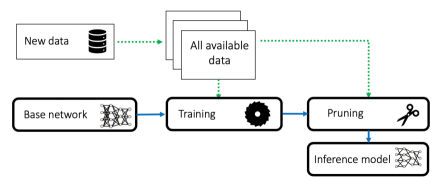
Figure 5: Illustration of the training-from-scratch approach.

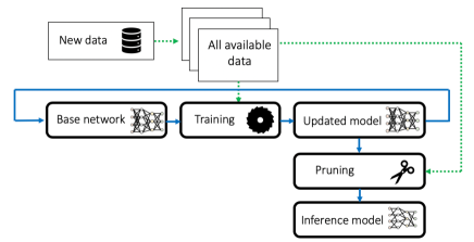
Figure 6: Illustration of the network fine-tunning approach.

We provide details of the experimental settings and results next.

5.1 LeNets on MNIST

We first show the effectiveness of our proposed methodology using LeNet-300-100 and LeNet-5 on the MNIST dataset.

TABLE IV: Experimental results for LeNet-300-100 on the MNIST dataset

Training	Error rate (%)			#Parameters (K)			#Training epochs
data used	TFS	NFT	Ours	TFS	NFT	Ours	TFS	NFT	Ours
10%	2.27	2.27	2.19	19.4	19.4	13.9	141	141	166
20%	1.80	1.84	1.70	22.7	20.5	17.6	131	136	109
30%	1.66	1.68	1.60	23.9	21.5	17.0	136	130	93
40%	1.63	1.62	1.55	20.5	22.7	13.8	131	124	79
50%	1.58	1.66	1.51	26.5	23.9	17.0	135	135	85
60%	1.43	1.51	1.39	27.8	29.3	26.5	140	109	71
70%	1.41	1.42	1.35	25.1	26.5	21.2	139	133	70
80%	1.41	1.42	1.36	29.3	27.8	21.1	141	127	66
90%	1.41	1.43	1.33	27.8	30.9	20.8	134	124	58
100%	1.40	1.41	1.33	31.3	32.5	21.7	137	131	49

TABLE V: Experimental results for LeNet-5 on the MNIST dataset

Training	Error rate (%)			#Parameters (K)			#Training epochs
data used	TFS	NFT	Ours	TFS	NFT	Ours	TFS	NFT	Ours
10%	1.62	1.62	1.45	5.3	5.3	4.9	148	148	162
20%	1.28	1.30	1.23	5.9	6.5	5.5	141	126	110
30%	1.01	1.05	0.97	6.5	6.2	6.2	136	118	92
40%	0.97	0.99	0.92	6.5	6.8	5.9	151	134	80
50%	0.95	1.00	0.93	7.2	6.8	6.0	135	141	83
60%	0.93	0.97	0.90	8.8	7.6	7.5	120	119	69
70%	0.90	0.94	0.87	8.0	8.4	6.3	129	99	66
80%	0.90	0.90	0.87	7.6	8.8	7.1	131	119	52
90%	0.88	0.91	0.87	10.9	9.8	7.9	124	127	56
100%	0.88	0.90	0.83	10.3	10.2	7.9	129	115	43

Architectures: We target two different base networks in the experiments: LeNet-300-100 and LeNet-5. These two networks were proposed in [37]. LeNet-300-100 is an MLP neural network. It has two hidden layers with 300 and 100 neurons each. LeNet-5 is a CNN with four hidden layers [two convolutional and two fully-connected (FC) layers]. The two convolutional layers share the same kernel size of 5$\times$5 and contain 6 and 16 filters, respectively, whereas the two FC layers have 120 and 84 neurons, respectively. The total number of network parameters in LeNet-300-100 and LeNet-5 is 266K and 59K, respectively.

Dataset: We report results on the MNIST dataset [37]. It has 70K (60K for training and 10K for testing) hand-written digit images of size 28$\times$28. We randomly reserve 5K images from the training set to build the validation set. We introduce affine distortions to the training instances for data augmentation, same as in [37].

Training: We split the training set (with 55K images) randomly into ten different parts of equal size. In the incremental learning experiments, we start with one part to train the initial model for subsequent updates. We then add one part as new data each time in the incremental learning scenario. For each update, we perform growth on new data and all data for 15 epochs and 20 epochs in the growth phase, respectively. Then, we prune the post-growth network for compactness. As for the two baselines (TFS and NFT), we train the model for 60 epochs, then prune the model iteratively. Note that all the models share the same recoverable pruning policy for a fair comparison of model size.

We compare the test error rate, number of parameters, and number of training epochs for the three approaches on LeNet-300-100 and LeNet-5 in Table IV and Table V, respectively. We execute incremental learning ten times in our experiments. In all the cases except the first round, our proposed method simultaneously delivers higher accuracy, reduced or equal model size, and less training cost relative to both baseline approaches. For example, when we add the last 10% training data to the existing 90% data, our grow-and-prune paradigm based incremental learning algorithm leads to 0.07% (0.08%) absolute accuracy gain, 31% (33%) model size reduction, and 64% (63%) training cost reduction compared to the conventional TFS (NFT) approach on LeNet-300-100. We observe similar improvements on LeNet-5.

Note that our incremental learning framework has higher training cost for the initial model (where only 10% training data are available). This is as expected since there is no existing model or knowledge for the initial model to start from, and thus all three approaches have to employ random initialization and start from scratch (TFS is equivalent to NFT in this case). However, whenever a pre-trained model with existing knowledge is available, our incremental learning approach always produces reduced training cost due to its capability of preserving existing knowledge effectively and distilling knowledge from new data efficiently.

5.2 ResNet-18 on ImageNet

TABLE VI: Experimental results for ResNet-18 on the ImageNet dataset

Training	Top-5 error rate (%)			#Parameters (M)			#Training epochs
data used	TFS	NFT	Ours	TFS	NFT	Ours	TFS	NFT	Ours
10%	30.40	30.40	30.36	2.8	2.8	1.9	229	229	269
20%	21.48	21.52	21.37	2.9	3.0	2.1	239	232	221
30%	17.88	17.90	17.78	3.1	2.8	2.5	204	209	170
40%	15.50	15.49	15.44	3.3	2.9	2.4	227	217	159
50%	14.09	14.17	14.03	3.5	3.5	2.6	260	240	130
60%	12.77	12.90	12.70	3.5	3.5	2.9	231	195	139
70%	12.17	12.31	12.15	3.9	4.1	3.3	198	206	109
80%	11.51	11.52	11.47	3.9	4.1	3.4	207	199	99
90%	11.47	11.64	11.44	4.3	4.9	3.3	259	187	92
100%	11.25	11.27	11.12	4.7	5.2	3.9	241	213	86

We now scale up the network architecture to ResNet-18 and the dataset to ImageNet, which is a widely-used benchmark for image recognition.

Architecture: ResNet is a milestone CNN architecture [13]. The introduced residual connections alleviate the exploding and vanishing gradient problem in the training of DNNs with large depth, and yield substantial accuracy improvements. We use ResNet-18 as the base network in our experiment. It has 17 convolutional layers and one FC layer. The total number of parameters in ResNet-18 is 11.7M.

Dataset: We report the results on the ImageNet dataset [7]. This is a large-scale dataset for image-classifying DNNs. It has 1.2M and 50K images from 1,000 distinct categories for training and validation, respectively. Since there is no publicly available test set, we randomly withhold 50 images from each class in the training set to build a validation set (50K images in all), and use the original validation set as the test set. We report the test accuracy in our experiment.

Training: Similar to the previous experiments on the MNIST dataset, we separate the training set evenly and randomly into ten different chunks. We use one chunk as the initially available data and add one chunk as new data each time. We perform growth on new data and all data for 20 epochs and 30 epochs in the growth phase in our proposed approach, respectively. We train the model for 90 epochs for the two baselines. In the pruning phase, all methods share the same recoverable pruning policy for a fair model size comparison.

Table VI compares three different metrics (top-5 error rate, number of parameters, and number of training epochs) for the three different approaches. Our proposed approach again outperforms both baselines except the training cost for the initial model. For example, it achieves up to 64% (60%) training cost reduction for model update compared to the TFS (NFT) approach, while delivering 0.13% (0.15%) higher top-5 accuracy, and 17% (25%) smaller model size at the same time.

5.3 DeepSpeech2 on AN4

TABLE VII: Experimental results for DeepSpeech2 with H-LSTM on the AN4 dataset

Training	WER (%)			#Parameters (M)			#Training epochs
data used	TFS	NFT	Ours	TFS	NFT	Ours	TFS	NFT	Ours
40%	48.1	48.1	45.8	4.8	4.8	4.0	267	267	313
50%	35.6	37.7	34.7	4.7	5.1	4.0	251	241	189
60%	33.9	34.0	32.4	5.5	5.3	4.4	281	220	160
70%	25.1	23.5	22.9	6.0	6.0	5.2	247	249	127
80%	20.9	21.8	20.1	5.9	6.7	4.8	230	196	129
90%	15.8	15.3	15.4	7.0	8.2	5.7	272	219	101
100%	12.4	12.6	11.7	7.4	7.6	5.7	269	232	88

We now consider another important machine learning application: speech recognition. We target the DeepSpeech2 [2] architecture with an H-LSTM on the AN4 dataset [40], and provide experimental details next.

Architecture: DeepSpeech2 is a popular architecture for speech recognition. It has three convolutional layers, three recurrent layers, one FC layer, and one connectionist temporal classification layer [15]. The inputs of the network are Mel-frequency cepstral coefficients of the sound power spectrum. We use bidirectional H-LSTM recurrent layers in our experiments and set the hidden state width for the H-LSTM cells to 800, same as reported in [15]. We introduce a dropout ratio of 0.2 for the hidden layers in the H-LSTM cells.

Dataset: The speech recognition dataset in our experiment is the AN4 dataset [40], which has 948 and 130 utterances for training and validation, respectively. We randomly reserve 100 utterances from the training set as the validation set, and use the original validation set as the test set.

Training: We first divide the training set evenly and randomly into ten different parts. We start with training an initial model based on partial training data, and then update the model based on the remaining parts. To train an initial model with acceptable accuracy, we find the minimum amount of training data to be 40% of all available training data (i.e., four parts). A decrease in this amount leads to an abrupt drop in accuracy ($>$80% WER when only three parts are used). Then, we add one part each time to update the model. For the model growth phase, we first grow the network for 20 epochs based on only the newly added data, and then 30 epochs when the new part is merged with existing ones. We train the model for 120 epochs for both conventional baselines. We conduct recoverable pruning for all the methods in pursuit of model compactness.

We compare the WER and number of parameters for the models derived from the three different approaches as well as their corresponding training epochs in Table VII. We observe a significant improvement in the trade-offs among accuracy, model size, and training cost in our proposed incremental learning framework. For example, when we add the last 10% training data, our model achieves 0.7% (0.9%) lower WER and 30% (33%) additional compression ratio with 67% (62%) less training cost compared to the TFS (NFT) approach.

6 Discussions

In this section, we discuss the learning mechanism of human brains and the underlying inspirations of our proposed incremental learning framework.

Our brains are plastic. They continually remold numerous synaptic connections as we acquire new knowledge and information [41]. Recent discoveries in neuroscience have unveiled the fact that our brain’s synaptic connections change every second over our entire lifetime. Furthermore, it has been shown that most new knowledge acquisition and information learning process in our brains result from the brain remodeling and synaptic connection rewiring mechanism (referred to as ‘neuroplasticity’) [41]. This is very different from the current DNNs that have fixed architectures with weights trained only with back-propagation to distill intelligence from a dataset.

To mimic the learning mechanism of human brains, we utilize gradient-based growth and magnitude-based pruning to train DNN architectures in our framework. During training, we adaptively adjust the connectivity of synaptic connections for the model to accommodate previously unseen data and acquire new knowledge. Such a brain-inspired algorithm delivers an efficient and accurate inference model at a significantly reduced learning cost. Future work could entail dynamic rewiring to adapt DNN depth as well as architecture learning for arbitrary feedforward neural networks.

7 Conclusions

In this paper, we proposed a brain-inspired incremental learning framework based on a grow-and-prune paradigm. We combine gradient-based growth and magnitude-based pruning in the model update process. We show the effectiveness and efficiency of our proposed methodology for different tasks on different datasets. For LeNet-300-100 (LeNet-5) on the MNIST dataset, we cut down the training cost by up to 64% (67%) compared to the TFS approach and 63% (63%) compared to the NFT approach. For ResNet-18 on the ImageNet dataset (DeepSpeech2 on the AN4 dataset), we reduce the training epochs by up to 64% (67%) compared to the TFS approach and 60% (62%) compared to the NFT approach. The derived models have improved accuracy (or reduced error rate) and more compact network architecture.

References

- [1] A. Krizhevsky, I. Sutskever, and G. E. Hinton, “ImageNet classification with deep convolutional neural networks,” in Proc. Advances in Neural Information Processing Systems, 2012, pp. 1097–1105.
- [2] D. Amodei, S. Ananthanarayanan, R. Anubhai, J. Bai, E. Battenberg, C. Case, J. Casper, B. Catanzaro, Q. Cheng, G. Chen et al., “Deep speech 2: End-to-end speech recognition in English and Mandarin,” in Proc. Int. Conf. Machine Learning, 2016, pp. 173–182.
- [3] H. Zhang, P.-H. Chen, and P. Ramadge, “Transfer learning on fMRI datasets,” in Proc. Int. Conf. Artificial Intelligence and Statistics, 2018.
- [4] P.-H. Chen, X. Zhu, H. Zhang, J. S. Turek, J. Chen, T. L. Willke, U. Hasson, and P. Ramadge, “A convolutional autoencoder for multi-subject fMRI data aggregation,” arXiv preprint arXiv:1608.04846, 2016.
- [5] I. Sutskever, O. Vinyals, and Q. V. Le, “Sequence to sequence learning with neural networks,” in Proc. Advances in Neural Information Processing Systems, 2014, pp. 3104–3112.
- [6] S. Arik, J. Chen, K. Peng, W. Ping, and Y. Zhou, “Neural voice cloning with a few samples,” in Proc. Advances in Neural Information Processing Systems, 2018, pp. 10 019–10 029.
- [7] J. Deng, W. Dong, R. Socher, L.-J. Li, K. Li, and F.-F. Li, “ImageNet: A large-scale hierarchical image database,” in Proc. IEEE Conf. Computer Vision and Pattern Recognition, 2009, pp. 248–255.
- [8] R. Istrate, A. C. I. Malossi, C. Bekas, and D. Nikolopoulos, “Incremental training of deep convolutional neural networks,” arXiv preprint arXiv:1803.10232, 2018.
- [9] H. Yin and N. K. Jha, “A health decision support system for disease diagnosis based on wearable medical sensors and machine learning ensembles,” IEEE Trans. Multi-Scale Computing Systems, vol. 3, no. 4, pp. 228–241, 2017.
- [10] R. Polikar, L. Upda, S. S. Upda, and V. Honavar, “Learn++: An incremental learning algorithm for supervised neural networks,” IEEE Trans. Systems, Man, and Cybernetics, vol. 31, no. 4, pp. 497–508, 2001.
- [11] S. Han, J. Pool, J. Tran, and W. J. Dally, “Learning both weights and connections for efficient neural network,” in Proc. Advances in Neural Information Processing Systems, 2015, pp. 1135–1143.
- [12] K. Simonyan and A. Zisserman, “Very deep convolutional networks for large-scale image recognition,” arXiv preprint arXiv:1409.1556, 2014.
- [13] K. He, X. Zhang, S. Ren, and J. Sun, “Deep residual learning for image recognition,” in Proc. IEEE Conf. Computer Vision and Pattern Recognition, 2016, pp. 770–778.
- [14] Y. Lin, S. Han, H. Mao, Y. Wang, and W. J. Dally, “Deep gradient compression: Reducing the communication bandwidth for distributed training,” arXiv preprint arXiv:1712.01887, 2017.
- [15] X. Dai, H. Yin, and N. K. Jha, “Grow and prune compact, fast, and accurate LSTMs,” arXiv preprint arXiv:1805.11797, 2018.
- [16] J. Yosinski, J. Clune, Y. Bengio, and H. Lipson, “How transferable are features in deep neural networks?” in Proc. Advances in Neural Information Processing Systems, 2014, pp. 3320–3328.
- [17] Z. Li and D. Hoiem, “Learning without forgetting,” IEEE Trans. on Pattern Analysis and Machine Intelligence, vol. 40, no. 12, pp. 2935–2947, 2018.
- [18] Z. Yan, H. Zhang, R. Piramuthu, V. Jagadeesh, D. DeCoste, W. Di, and Y. Yu, “HD-CNN: Hierarchical deep convolutional neural networks for large scale visual recognition,” in Proc. IEEE Int. Conf. Computer Vision, 2015, pp. 2740–2748.
- [19] T. Chen, I. Goodfellow, and J. Shlens, “Net2Net: Accelerating learning via knowledge transfer,” arXiv preprint arXiv:1511.05641, 2015.
- [20] T. Xiao, J. Zhang, K. Yang, Y. Peng, and Z. Zhang, “Error-driven incremental learning in deep convolutional neural network for large-scale image classification,” in Proc. ACM Int. Conf. on Multimedia. ACM, 2014, pp. 177–186.
- [21] D. Roy, P. Panda, and K. Roy, “Tree-CNN: A hierarchical deep convolutional neural network for incremental learning,” arXiv preprint arXiv:1802.05800, 2018.
- [22] A. A. Rusu, N. C. Rabinowitz, G. Desjardins, H. Soyer, J. Kirkpatrick, K. Kavukcuoglu, R. Pascanu, and R. Hadsell, “Progressive neural networks,” arXiv preprint arXiv:1606.04671, 2016.
- [23] A. V. Terekhov, G. Montone, and J. K. O’Regan, “Knowledge transfer in deep block-modular neural networks,” in Proc. Conf. Biomimetic and Biohybrid Systems. Springer, 2015, pp. 268–279.
- [24] M. Sandler, A. Howard, M. Zhu, A. Zhmoginov, and L.-C. Chen, “MobilenetV2: Inverted residuals and linear bottlenecks,” in Proc. IEEE Conf. Computer Vision and Pattern Recognition, 2018, pp. 4510–4520.
- [25] N. Ma, X. Zhang, H.-T. Zheng, and J. Sun, “Shufflenet V2: Practical guidelines for efficient CNN architecture design,” in Proc. European Conf. Computer Vision, 2018, pp. 116–131.
- [26] B. Wu, A. Wan, X. Yue, P. Jin, S. Zhao, N. Golmant, A. Gholaminejad, J. Gonzalez, and K. Keutzer, “Shift: A zero FLOP, zero parameter alternative to spatial convolutions,” in Proc. IEEE Conf. Computer Vision and Pattern Recognition, 2018, pp. 9127–9135.
- [27] M. Tan, B. Chen, R. Pang, V. Vasudevan, and Q. V. Le, “MnasNet: Platform-aware neural architecture search for mobile,” arXiv preprint arXiv:1807.11626, 2018.
- [28] X. Dai, P. Zhang, B. Wu, H. Yin, F. Sun, Y. Wang, M. Dukhan, Y. Hu, Y. Wu, Y. Jia, P. Vajda, M. Uyttendaele, and N. K. Jha, “ChamNet: Towards efficient network design through platform-aware model adaptation,” in Proc. IEEE Conf. Computer Vision and Pattern Recognition, 2019.
- [29] S. Hassantabar, Z. Wang, and N. K. Jha, “SCANN: Synthesis of compact and accurate neural networks,” arXiv preprint arXiv:1904.09090, 2019.
- [30] X. Dai, H. Yin, and N. K. Jha, “NeST: A neural network synthesis tool based on a grow-and-prune paradigm,” IEEE Trans. on Computers, 2019.
- [31] W. Wen, C. Wu, Y. Wang, Y. Chen, and H. Li, “Learning structured sparsity in deep neural networks,” in Proc. Advances in Neural Information Processing Systems, 2016, pp. 2074–2082.
- [32] H. Yin, G. Chen, Y. Li, S. Che, W. Zhang, and N. K. Jha, “Hardware-guided symbiotic training for compact, accurate, yet execution-efficient LSTM,” arXiv preprint arXiv:1901.10997, 2019.
- [33] S. Han, H. Mao, and W. J. Dally, “Deep compression: Compressing deep neural networks with pruning, trained quantization and Huffman coding,” arXiv preprint arXiv:1510.00149, 2015.
- [34] C. Zhu, S. Han, H. Mao, and W. J. Dally, “Trained ternary quantization,” arXiv preprint arXiv:1612.01064, 2016.
- [35] S. S. Sarwar, A. Ankit, and K. Roy, “Incremental learning in deep convolutional neural networks using partial network sharing,” arXiv preprint arXiv:1712.02719, 2017.
- [36] S. Grossberg, “Nonlinear neural networks: Principles, mechanisms, and architectures,” Neural Networks, vol. 1, no. 1, pp. 17–61, 1988.
- [37] Y. Lecun, L. Bottou, Y. Bengio, and P. Haffner, “Gradient-based learning applied to document recognition,” Proceedings of the IEEE, vol. 86, no. 11, pp. 2278–2324, 1998.
- [38] H. Yin, Z. Wang, and N. K. Jha, “A hierarchical inference model for Internet-of-Things,” IEEE Trans. Multi-Scale Computing Systems, vol. 4, no. 3, pp. 260–271, 2018.
- [39] A. Paszke, S. Gross, S. Chintala, G. Chanan, E. Yang, Z. DeVito, Z. Lin, A. Desmaison, L. Antiga, and A. Lerer, “Automatic differentiation in PyTorch,” NIPS Workshop Autodiff, 2017.
- [40] A. Acero, “Acoustical and environmental robustness in automatic speech recognition,” in Proc. IEEE Int. Conf. Acoustic, Speech, and Signal Processing, 1990.
- [41] S. N. Burke and C. A. Barnes, “Neural plasticity in the ageing brain,” Nature Reviews Neuroscience, vol. 7, no. 1, p. 30, 2006.