HVAC Energy Cost Optimization for a Multi-zone Building via A Decentralized Approach

Abstract

It has been well acknowledged that buildings account for a large proportion of the world’s energy consumption. However, the energy use of buildings, especially the heating, ventilation and air-conditioning (HVAC), is far from being efficient. There still exists a dramatic potential to save energy through improving building energy efficiency. Therefore, this paper studies the control of HVAC system for multi-zone buildings with the objective to reduce energy consumption cost while satisfying thermal comfort. In particular, the thermal couplings due to the heat transfer between the adjacent zones are incorporated in the optimization. Considering that a centralized method is generally computationally prohibitive for large buildings, an efficient decentralized approach is developed, based on the Accelerated Distributed Augmented Lagrangian (ADAL) method [1]. To evaluate the performance of the proposed method, we first compare it with a centralized method, in which the optimal solution of a small-scale problem can be obtained. We find that this decentralized approach can almost approach the optimal solution of the problem. Further, this decentralized approach is compared with the Distributed Token-Based Scheduling Strategy (DTBSS) [2]. The numeric results reveal that when the number of zones is relatively small (less than 20), the two decentralized methods can achieve a comparable performance regarding the cost of the HVAC system. However, with an increase of the number of zones in the building, the proposed decentralized approach demonstrates better performance with a considerable reduction of the total cost. Moreover, the decentralized approach proposed in this paper demonstrate better scalability with less average computation required.

Note to Practitioners

Buildings accounts for a large proportion of the world’s energy consumption, especially the HVAC system. How to improve the energy efficiency of HVAC system has been recognized as an important and urgent problem for a sustainable future. Motivated by this important problem, this paper is focused on the intelligent control of HVAC system for multi-zone buildings with the objective to reduce energy consumption cost for the HVAC system while maintaining zone thermal comfort. Considering that a centralized method usually encounters computation difficulties with a large number of zones, this paper aims to develop an efficient decentralized solution. In terms of the problem, there usually exist various couplings between different zones, which both arise from the heat transfer between the neighbouring zones and the operation limits of the HVAC system. Moreover, this problem is nonconvex and nonlinear. Therefore, it is generally difficult to find an existing decentralized or distributed method, which are mostly established for convex optimization problems. Motivated by the recent progress on decentralized or distributed optimization for nonconvex problems, this paper proposes an efficient decentralized approach, which mainly contains three steps. In the first step, the original optimization problem is relaxed by introducing some auxiliary decision variables. In the relaxed optimization problem, there only exist linear constraints, however, the recursive feasibility of the solution can’t be guaranteed. In the second step, the ADAL method [1] is applied to solve the relaxed optimization problem in a decentralized manner. Specifically, each individual zone can determine its local decision variables by solving a small-scale subproblem in parallel at each iteration. In the last step, a heuristic methods is proposed to recover the recursive feasibility of the solution for the original optimization problem by exploring the structures of the problem. In this paper, the performance of this decentralized approach is first evaluated through comparison with a centralized method, in which the optimal solution can be obtained. We find that this decentralized approach can almost approach the optimal solution of the problem. Moreover, we compare the decentralized approach with the DTBSS method [2]. The numeric results reveal that the decentralized approach proposed in this paper demonstrates better performance both in reducing the cost of the HVAC systems as well as in improving the computational efficiency when the number of zones is large.

I Introduction

It has been well acknowledged that buildings are responsible for a large proportion of the world’s energy consumption. Specifically, about $40\%$ of the primal energy and $70\%$ of the electricity is consumed in buildings [3]. In particular, about $40\%$-$50\%$ of this consumption is attributed to heating, ventilation and air-conditioning (HVAC) systems [3]. In tropical countries, like Singapore, Malaysia, and India etc., the proportion of energy consumption caused by HVAC is even higher [2]. However, the energy consumption in buildings, especially the HVAC systems, is far from being efficient. There still exists dramatic potential to reduce unnecessary energy consumption through improving building energy efficiency [2].

Over the years, the control of HVAC systems and the management of building energy systems have been extensively investigated via various methods including model predictive control (MPC) [4, 5, 6, 7], mixed-integer linear programming (MILP) [8, 9], sequential quadratic programming (SQP) [10, 11, 12], intelligent control based on fuzzy logic or genetic algorithm [13, 14, 15], and rule-based methods [16, 17]. However, most of these methods are carried out in a centralized manner. For large buildings with multiple zones, these methods can be computationally prohibitive or not scalable. Therefore, to deal with such situation, this paper focuses on developing an efficient decentralized approach for thermal comfort control of HVAC systems for large multi-zone buildings.

It’s challenging to achieve optimal control of an HVAC system. For multi-zone buildings, where a number of thermal zones share a central HVAC system, the problem is more complicated and challenging. First, there exist various decision variables. Both the temperature and mass flow rates for all zones need to be coordinated to save energy while satisfying the indoor thermal comfort requirements. Second, there exist various couplings between different thermal zones. The couplings both arise from the heat transfer between the adjacent zones and the operation limits of the HVAC system. Therefore, there usually exist various temporally and spatially coupled constraints. Third, the problem is nonlinear and nonconvex. More specifically, both the system dynamics and the global objective function of the problem are nonlinear and nonconvex. Most of the existing decentralized or distributed methods, such as distributed primal-dual subgradient methods [18], dual decomposition [19], distributed Alternating Direction Method of Multipliers (ADMM) [20] can’t be directly applied to solve the problem. Because these decentralized or distributed methods are generally established for convex problems and some of them even can only accommodate linear constraints.

This paper investigates the control of HVAC systems in multi-zone buildings with the objective to reduce energy cost while guaranteeing indoor thermal comfort, which incorporates the thermal couplings due to heat transfer between adjacent zones. The main contributions of the paper are summarized as follows. Based on decentralized optimization for nonconvex problems with some special structures [1, 21], an efficient decentralized approach for the control of multi-zone HVAC systems is developed in this paper. This decentralized approach mainly contains three steps. Specifically, the first step is to relax the original optimization problem. This can be achieved by defining some auxiliary decision variables. In the relaxed optimization problem, there only exist linear constraints, however, the recursive feasibility of the solution can’t be guaranteed. In the second step, an Accelerated Distributed Augmented Lagrangian (ADAL) method proposed in [1] is applied to solve the nonconvex relaxed optimization problem with only linear constraints. Last but very important, the recursive feasibility of the solution is recovered from the optimal solution of the relaxed optimization problem through an heuristic method. In this decentralized approach, all thermal zones can determine their own mass flow rates and zone temperature by solving local subproblems in parallel at each iteration, therefore this method is scalable to large buildings with a large number of zones. To evaluate the performance of this decentralized approach, we first compare it with a centralized method, in which the optimal solution can be obtained. We find that the decentralized approach can almost approach the optimal solution of the problem. Moreover, this decentralized approach is compared with a distributed Token-Based Scheduling Strategy (TBSS) proposed in [2]. The numeric results demonstrate that when the number of zones is relatively small (less than $20$), the decentralized approach can achieve a comparable performance compared with the distributed TBSS method with about $2\%\sim 4\%$ reduction of the cost. However, the decentralized approach outperforms the distributed TBSS both in reducing the cost of the HVAC system and in reducing the average computation with a large number of zones in the building.

The remainder of this paper is outlined as follows. In Section II, the related works regarding the decentralized or distributed control of HVAC systems for multi-zone buildings are reviewed. In Section III, the problem formulation is presented. In Section IV, the decentralized approach is introduced. In Section V, the performance and scalability of the decentralized approach is validated through case studies. In Section VI, we briefly conclude this paper.

II Related Works

As aforementioned, there already exist various centralized methods for control of HVAC systems. However, decentralized or distributed methods for the control of HVAC system in multi-zone buildings have not been well studied. Generally, the existing decentralized or distributed methods can be divided into two categories based on the decision variables. The first category is mainly focused on zone temperature regulation [22, 23, 24]. In this category of works, the zone temperature are regarded as the decision variables. However, how to control the HVAC systems to achieve the desired zone temperature is circumvented and not discussed. In these studies, the zone temperature dynamics are usually assumed to be linear and the problems are convex. Decentralized methods based on decoupling [22], incentive price [23] and Dantzig-Wolf decomposition [24] have been applied to solve the problems. In the other category, the control of the HVAC system is directly discussed. In this case, the thermal dynamic of each individual zone is usually nonlinear, which not only depends on its own local decision variables but also depends on those of the adjacent zones due to thermal couplings. The problem is usually very complicated and difficult. In the literature, most of the existing works ignore the thermal couplings between the adjacent zones [25, 26]. In [25], a real-time decentralized algorithm based on Lyapunov optimization and some approximation techniques was proposed. In [26], to protect privacy, a decentralized method based on a multi-level virtual market was proposed. Different from the above works where the heat transfer between neighbouring thermal zones is ignored, [2, 27] regarded the heat transfer from the adjacent zone as external thermal disturbances that are measured through sensors or learned from data at the beginning of each planning horizon. To cope with the difficulties and challenges to solve the problem, a hierarchical distributed method was proposed, in which the original optimization problem was divided into three-level subproblems and each corresponds to a part of the global objective function. Different from those mentioned above, [28, 29] studied the steady-state temperature regulation of the HVAC system for an energy-efficient building via a decentralized primal-dual gradient method while relaxing the global objective function. The problem was formulated as a static optimization problem without considering the thermal dynamics and the thermal coupling among the neighboring zones.

Generally speaking, in most of the related works, the thermal couplings among the neighbouring or adjacent zones are ignored or not explicitly considered, which may lead to the degradation of performance in practice. On one hand, the actual energy cost of HVAC may rise due to the heat transfer between the neighbouring zones ignored in the optimization. On the other hand, the realistic thermal condition of each individual zone may deviate from the comfortable range. An attempt was reported in [30], which studied the distributed MPC strategy for HVAC system in a multi-zone building, where the thermal couplings between the neighbouring zones are explicitly discussed. To cope with the difficulties due to the nonlinearity and nonconvexity, a distributed ADMM method was applied based on some convexity approximation.

Complementary to the existing works, this paper considers the thermal couplings among the neighbouring zones. To improve scalability of the method, an efficient decentralized approach based on ADAL is developed.

III Problem Formulation

III-A HVAC Systems for Multi-zone Buildings

A typical schematic of an HVAC system in a multi-zone building is shown in Fig. 1. The main parts of the system include the Air Handling Unit (AHU), the Variable Air Volume (VAV) box, and the chiller. The central AHU is shared by multi-zones, which is equipped with a damper, a cooling/heating coil and a supply fan. The damper is responsible for mixing the return air from inside and the freash air from outside. The heating/cooling coil can cool down/heat up the mixed air to a setpoint temperature. Without loss of generality, this paper considers the cooling mode of the HVAC system. Generally, the temperature of the supply air out of AHU is $12$-$16^{\circ}$C in the cooling mode. Besides, there is a local VAV box related to each zone, which consists of a damper and a heating coil. This damper can regulate air flow rate supplied to the zone, while the heating coil can reheat the supply air before supplied to the zone if necessary (in this paper, the heating coil of the local VAV box is not discussed). More details regarding HVAC systems for multi-zone buildings can refer to [10, 29].

In terms of the control of HVAC systems in multi-zone buildings, one important problem is how to improve energy efficiency while satisfying the thermal comfort of each zone. This problem is complicated and difficult due to the various couplings between different zones. On one hand, the thermal dynamics of different zones are usually coupled with each other due to heat transfer. On the other hand, the control of the HVAC system shared by different zones is generally coupled by the operation limits and the nonlinear energy consumption cost of the system.

In this paper, the problem is discussed in a discrete-time framework. The optimization horizon (one day) is equally divided into $T=48$ stages, each corresponding to a decision interval of $\Delta_{t}=30$ mins.

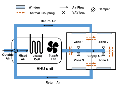
Figure 1: The schematic of an HVAC system in a multi-zone building.

III-B Zone Thermal Dynamics

In this paper, we consider a multi-zone building with $I$ thermal zones, which are indexed by $\mathcal{I}=\{1,2,\cdots,I\}$. The control of the HVAC system over the optimization horizon $\mathcal{T}=\{0,1,\cdots,T-1\}$ is studied. The thermal dynamics of zone $i$ ($\forall i\in\mathcal{I}$) can be described based on the Resistance-Capacitance (RC) network [31, 32], i.e.,

$$\begin{split}C_{i}(T^{i}_{t+1}&-T^{i}_{t})=\sum_{j\in\mathcal{N}_{i}}\frac{T^{j}_{t}-T^{i}_{t}}{R_{ij}}\Delta_{t}\\ &+\frac{T^{o}_{t}-T^{i}_{t}}{R_{oi}}\Delta_{t}+c_{p}m^{zi}_{t}(T^{c}_{t}-T^{i}_{t})\Delta_{t}+Q^{i}_{t}\Delta_{t}\end{split}$$ (1)

where $C_{i}$ is the heat capacity of the indoor air in zone $i$. $T^{i}_{t}$ is the temperature of zone $i$ at time $t$. $T^{o}_{t}$ denotes the outside air temperature at time $t$. $R_{oi}$ is the thermal resistance of the window between zone $i$ and the outside. $R_{ij}$ denotes the thermal resistance between zone $i$ and zone $j$. $\mathcal{N}_{i}$ denotes the collection of adjacent zones of zone $i$. $c_{p}$ is the specific heat of air. $m^{zi}_{t}$ denotes the air flow rate supplied to zone $i$. $Q^{i}_{t}$ denotes the total heat generation in zone $i$, which may result from occupants, devices and solar radiation, etc.

If we define $A^{ii}=1-(\sum_{j\in\mathcal{N}_{i}}\frac{\Delta_{t}}{R_{ij}C_{i}}+\frac{\Delta_{t}}{C_{i}R_{oi}})$, $A^{ij}=\frac{\Delta_{t}}{C_{i}R_{ij}}$, $C^{ii}=-\frac{\Delta_{t}\cdot c_{p}}{C_{i}}$, and $D^{ii}_{t}=\frac{\Delta_{t}T^{o}_{t}}{C_{i}R_{oi}}+\frac{\Delta_{t}\cdot Q^{i}_{t}}{C_{i}}$. the zone thermal dynamics in (1) can be equivalently described as

$$T^{i}_{t+1}=A^{ii}T^{i}_{t}+\sum_{j\in\mathcal{N}_{i}}A^{ij}T^{j}_{t}+C^{ii}m^{zi}_{t}(T^{i}_{t}-T^{c}_{t})+D^{ii}_{t}$$ (2)

III-C The AHU

As introduced in Section II-A, the AHU is responsible for cooling down the mixed air to a setpoint temperature before supplied to each individual zone. The main parameters related to the AHU include 1) $d_{r}$ ($0\!\leq\!d_{r}\!\leq\!1$): the fraction of the return air from inside. 2) $T^{r}_{t}$: the average temperature of the return air from inside. 3) $T^{m}_{t}$: the average temperature of the mixed air before supplied to the AHU. 4) $T^{c}_{t}$: the setpoint temperature of the suppy air by the AHU. The settings of $d_{r}$ and $T^{c}_{t}$ are usually determined based on experience. The average temperature of the return air from inside at time $t$ is determined by

$$\begin{split}T^{r}_{t}=\frac{\sum_{i=1}^{I}m^{zi}_{t}T^{i}_{t}}{\sum_{i=1}^{I}m^{zi}_{t}}\end{split}$$ (3)

And the average temperature of the mixed air that supplied to the AHU at time $t$ can be determined by

$$\begin{split}T^{m}_{t}&=(1-d_{r})T^{o}_{t}+d_{r}T^{r}_{t}\\ &=(1-d_{r})T^{o}_{t}+d_{r}\frac{\sum_{i=1}^{I}m^{zi}_{t}T^{i}_{t}}{\sum_{i=1}^{I}m^{zi}_{t}}\end{split}$$ (4)

As aforementioned, the AHU is mainly composed of the cooling coil and the supply fan. Therefore, the main energy consumption of the AHU consists of two parts. The first part is caused by the cooling coil, which can be determined by

$$\begin{split}P^{c}_{t}=c_{p}\eta(\sum_{i=1}^{I}m^{zi}_{t})(T^{m}_{t}-T^{c}_{t})\end{split}$$ (5)

where $\eta$ is the reciprocal of the coefficient of performance (COP) of the chiller, which captures the ratio of provided heating or cooling to the total consumed electrical energy.

By substituting (4) into (5), we have

$$\begin{split}P^{c}_{t}\!\!=\!\!c_{p}\eta(1\!-\!d_{r})\!\!\sum_{i=1}^{I}\!m^{zi}_{t}\!(T^{o}_{t}\!-\!T^{c}_{t})\!+\!c_{p}\eta d_{r}\sum_{i=1}^{I}\!m^{zi}_{t}(T^{i}_{t}\!-\!T^{c}_{t})\\ \end{split}$$ (6)

From (6), we note that the cooling power of the AHU can be divided into two parts. The first part is to cool down the proportion of the outside fresh air to the setpoint temperature. And the second part is to cool down the proportion of the return air from inside.

The second part of the energy consumption results from the supply fan. According to [26] and [30], the energy consumption of the supply fan depends on the cube of the total zone air flow rate, i.e.,

$$\begin{split}P^{f}_{t}=\kappa_{f}(\sum_{i=1}^{I}m^{zi}_{t})^{3}\end{split}$$ (7)

where $\kappa_{f}$ is a fixed parameter that captures the efficiency of the supply fan.

Therefore, the total power consumed by the HVAC system at time $t$ can be calculated as

$$\begin{split}&P^{c}_{t}+P^{f}_{t}\!=\!c_{p}(1-d_{r})\sum_{i=1}^{I}m^{zi}_{t}(T^{o}_{t}-T^{c}_{t})\!\\ &\quad\quad\quad+\!c_{p}d_{r}\sum_{i=1}^{I}m^{zi}_{t}(T^{i}_{t}-T^{c}_{t})+\kappa_{f}(\sum_{i=1}^{I}{m^{zi}_{t}})^{3}\\ \end{split}$$ (8)

From (8), we note that the power consumption of the HVAC system is a nonlinear function with respect to the decision variables $m^{zi}_{t}$ and state variables $T^{i}_{t}$ of each individual zone $i$ ($i\in\mathcal{I}$).

III-D System Constraints

In terms of the control of the HVAC system in multi-zone building, there exist various constraints. First of all, the thermal comfort requirement of each individual zone should be guaranteed. In this paper, we use temperature ranges to describe the thermal comfort requirements of different zones, thus we have

$$\begin{split}\underline{T}^{i}&\leq T^{i}_{t}\leq\overline{T}^{i},\quad\forall i\in\mathcal{I},~{}t\in\mathcal{T}\end{split}$$ (9)

where $\underline{T}^{i}$ and $\overline{T}^{i}$ represent the lower and upper bound of the comfortable temperature for zone $i$, respectively. To accommodate personalized thermal comfort, $\underline{T}^{i}$ and $\overline{T}^{i}$ may be different for different zones.

Also, the zone air flow rate is usually bounded, i.e.,

$$\begin{split}&\underline{m}^{zi}\leq m^{zi}_{t}\leq\overline{m}^{zi},\quad\forall i\in\mathcal{I},~{}t\in\mathcal{T}\\ \end{split}$$ (10)

where $\underline{m}^{zi}$ and $\overline{m}^{zi}$ denote the lower and upper bound of the air flow rate for zone $i$, respectively. The lower and upper bound of the zone air flow rates are generally determined by the pressure supplied by the fan in the duct system [2].

Besides, there usually exist operation limits for the central AHU that shared by the multi-zones, i.e.,

$$\begin{split}&\sum_{i=1}^{I}m^{zi}_{t}\leq\overline{m},~{}\forall t\in\mathcal{T}\\ \end{split}$$ (11)

where $\overline{m}$ denotes the maximum total air flow rate that can be supplied by the AHU at the same time.

III-E The Optimization Problem

To improve energy efficiency, the problem is how to reduce the energy cost of the HVAC system while guaranteeing the thermal comfort of different zones. Therefore, the optimization problem can be described as follows.

$$\min_{m^{zi}_{t},T^{i}_{t}}J=\sum_{t=0}^{T-1}c_{t}\cdot\Big{\{}P^{c}_{t}+P^{f}_{t}\Big{\}}\cdot\Delta_{t}$$ (P1)

$$\textrm{{{Constraints:}}}~{}(\ref{zone temperature dynamics}),(\ref{temperature range})-(\ref{total air flow rate bound})\quad\quad$$

where $c_{t}$ denotes the electricity price at time $t$.

In (P1), the total energy consumption cost of the HVAC system over the optimization horizon $\mathcal{T}$ is selected as the global objective function. We note that this global objective function is non-separable and nondecomposable with respect to the thermal zones. Becides, there exist various coupled nonlinear constraints due to the thermal coupling among different zones and the operation limits of the HVAC system. The problem (P1) is a nonlinear and nonconvex optimization problem, which is difficult to find an existing decentralized or distributed method to solve it. Because most of the existing decentralized or distributed methods [33, 34, 35, 18, 19, 20], such as distributed primal-dual subgradient methods [18], dual decomposition [19], distributed ADMM [20] are developed for convex optimization problems and some of them can only tackle linear constraints.

IV Decentralized Approach

As aforementioned, it is challenging and nontrivial to find an existing decentralized or distributed solution method for (P1) due to the nonconvexity and nonlinearity of the problem. To cope with the difficulties, this paper proposes an efficient decentralized approach to solve problem (P1). Generally, this decentralized approach mainly contains three steps. In the first step, the original optimization problem (P1) is relaxed by introducing some appropriate auxiliary decision variables. For the relaxed optimization problem, there only exist linear (coupled and decoupled) constraints. However, the recursive feasibility of the solution cannot be guaranteed. In the second step, an ADAL method [1] is applied to solve the nonconvex relaxed optimization problem in a decentralized manner. Last but very important, the third step is focused on recovering the recursive feasibility of the solution for (P1).

To deal with the nonlinear constraints of problem (P1), we first introduce the following auxilliary decision variables, i.e., $X^{i}_{t}=m^{zi}_{t}(T^{i}_{t}-T^{c}_{t})\geq 0$ ($\forall i\in\mathcal{I},t\in\mathcal{T}$) and $Y_{t}=\sum_{i=1}^{I}m^{zi}_{t}$ ($\forall t\in\mathcal{T}$). We note that $X^{i}_{t}$ can be regarded as the “cooling power” supplied to zone $i$ at time $t$, and $Y_{t}$ can be regarded as the total air flow rate supplied by the AHU to all zones in the building at time $t$.

According to [36] and [30], these auxiliary decision variables $X^{i}_{t}$ ($\forall i\in\mathcal{I}$, $t\in\mathcal{T}$) are bounded by their convex and concave envelopes, respectively. Therefore, we have

$$\begin{split}&X^{i}_{t}=m^{zi}_{t}(T^{i}_{t}-T^{c}_{t})\\ &\!\geq\!\max\!\Big{\{}\underline{m}^{zi}\!(T^{i}_{t}\!-\!T^{c}_{t})\!+\!m^{zi}_{t}(\underline{T}^{i}\!-\!T^{c}_{t})\!-\!\underline{m}^{zi}(\underline{T}^{i}-T^{c}_{t}),\\ &\quad\quad\quad\overline{m}^{zi}(T^{i}_{t}\!-\!T^{c}_{t})\!+\!m^{zi}_{t}(\overline{T}^{i}\!-\!T^{c}_{t})\!-\!\overline{m}^{zi}(\overline{T}^{i}\!-\!T^{c}_{t})\Big{\}},\\ &X^{i}_{t}=m^{zi}_{t}(T^{i}_{t}-T^{c}_{t})\\ &\leq\min\Big{\{}m^{zi}_{t}(\overline{T}^{i}\!-\!T^{c}_{t})\!+\!\underline{m}^{zi}(T^{i}_{t}\!-\!T^{c}_{t})\!-\!\underline{m}^{zi}(\overline{T}^{i}\!-\!T^{c}_{t}),\\ &\quad\quad\quad\overline{m}^{zi}(T^{i}_{t}\!-\!T^{c}_{t})\!+\!m^{zi}(\underline{T}^{i}\!-\!T^{c}_{t})\!-\!\overline{m}^{zi}(\underline{T}^{i}-T^{c}_{t})\Big{\}},\\ &\quad\quad\quad\quad\forall i\in\mathcal{I},~{}t\in\mathcal{T}.\\ \end{split}$$ (12)

Therefore, by introducing these auxiliary decision variables, we can obtain the following relaxed optimization problem (P2) regarding the original optimization problem (P1):

$$\min_{m^{zi}_{t},T^{i}_{t},X^{i}_{t},Y_{t}}J=\sum_{t=0}^{T-1}c_{t}\cdot\Big{\{}c_{p}\eta(1-d_{r})(T^{o}_{t}-T^{c}_{t})Y_{t}\quad\quad\quad$$

$$\quad\quad\quad\quad\quad\quad+\kappa_{f}(Y_{t})^{3}+c_{p}\eta d_{r}\sum_{i=1}^{I}X^{i}_{t}\Big{\}}\cdot\Delta_{t}\quad$$ (P2)

subject to

$$T^{i}_{t+1}=A^{ii}T^{i}_{t}+\sum_{j\in\mathcal{N}_{i}}A^{ij}T^{j}_{t}+C_{ii}X^{i}_{t}+D^{ii}_{t},$$ (13a)

$$\underline{m}^{zi}\leq m^{zi}_{t}\leq\overline{m}^{zi},$$ (13b)

$$\underline{T}^{i}\leq T^{i}_{t}\leq\overline{T}^{i},$$ (13c)

$$X^{i}_{t}\!\geq\!\underline{m}^{zi}(\!T^{i}_{t}\!-\!T^{c}_{t})\!+\!m^{zi}_{t}(\underline{T}^{i}-T^{c}_{t})-\underline{m}^{zi}(\underline{T}^{i}-T^{c}_{t}),$$ (13d)

$$X^{i}_{t}\!\geq\!\overline{m}^{zi}(T^{i}_{t}-T^{c}_{t})\!+\!m^{zi}_{t}(\overline{T}^{i}\!-\!T^{c}_{t})\!-\!\overline{m}^{zi}(\overline{T}^{i}-T^{c}_{t}),$$ (13e)

$$X^{i}_{t}\!\leq\!m^{zi}_{t}(\overline{T}^{i}\!-\!T^{c}_{t})\!+\!\underline{m}^{zi}(T^{i}_{t}-T^{c}_{t})-\underline{m}^{zi}(\overline{T}^{i}-T^{c}_{t}),$$ (13f)

$$X^{i}_{t}\!\leq\!\overline{m}^{zi}(T^{i}_{t}-T^{c}_{t})\!+\!m^{zi}(\underline{T}^{i}\!-\!T^{c}_{t})\!-\!\overline{m}^{zi}(\underline{T}^{i}-T^{c}_{t}),$$ (13g)

$$\quad\quad\quad\quad\quad\forall i\in\mathcal{I},~{}t\in\mathcal{T}.$$

$$\sum_{i=1}^{I}m^{zi}_{t}\leq Y_{t},$$ (13h)

$$\sum_{i=1}^{I}m^{zi}_{t}\leq\overline{m},\forall t\in\mathcal{T}.$$ (13i)

In (P2), Constraints (13d)-(13g) correspond to Constraints (12), which relate to the auxiliary decision variable $X^{i}_{t}$. And Constraints (13h) relate to the auxiliary decision variable $Y_{t}$. We note that problem (P2) is still nonconvex due to the global objective function, however, there only exist linear constraints. This problem can be tackled by the ADAL method [1], which has been established for problems with nonconvex global objective function but with only linear coupled constraints. Therefore, in the second step, we apply the ADAL method to solve problem (P2) in a decentralized manner. More specifically, we assume that there are $I+1$ agents, which are indexed by $\mathcal{I}\cup\{0\}$. The collection of the agents $\mathcal{I}$ corresponds to the $I$ zones in the building. In addition, we define a virtual Agent $0$, to regulate the total air flow rate supplied by the AHU.

For each Agent $i$ that related to zone $i$ ($\forall i\in\mathcal{I}$), the local decision variables at time $t$ can be gathered as

$$\begin{split}\bm{x}^{i}_{t}=&\Big{(}T^{i}_{t},m^{zi}_{t},X^{i}_{t}\Big{)}^{T},~{}\forall i\in\mathcal{I},t\in\mathcal{T}.\end{split}$$ (14)

For Agent $0$, the local decision variable at time $t$ is defined as

$$\bm{x}^{0}_{t}=Y_{t},~{}\forall t\in\mathcal{T}.$$ (15)

For notation, we use the vectors $\bm{x}^{i}=[(\bm{x}^{i}_{0})^{T},(\bm{x}^{i}_{1})^{T},\cdots,$ $(\bm{x}^{i}_{T-1})^{T}]^{T}$ to represent the local decision variables of Agent $i$ ($\forall i\in\mathcal{I}\cup\{0\}$) over the optimization horizon $\mathcal{T}$.

Accordingly, the global objective function in (P2) can be decomposed with respect to the agents.

$$\begin{split}&\textrm{For $i\in\mathcal{I}$, we have }\\ &\quad\quad J_{i}(\bm{x}^{i})\!\!=\!\sum_{t=0}^{T-1}\!c_{t}\!\cdot\Big{\{}c_{p}\eta d_{r}\!X^{i}_{t}\!\Big{\}}\cdot\Delta_{t}\\ &\textrm{For $i=0$, we have}\\ &J_{0}(\bm{x}^{0})\!=\!\!\!\sum_{t=0}^{T-1}\!\!c_{t}\!\cdot\!\Big{\{}c_{p}\eta(1\!-\!d_{r})(T^{o}_{t}-T^{c}_{t})Y_{t}\!+\!\kappa_{f}(Y_{t})^{3}\Big{\}}\!\cdot\!\Delta_{t}\end{split}$$ (16)

It’s straightforward that $J=\sum_{i=0}^{I}J_{i}(\bm{x}^{i})$, where $J_{i}(\bm{x}^{i})$ can be regarded as the local objective function of Agent $i$.

Before we can apply the ADAL method to solve problem (P2), we first need to convert the problem to the specific structures as required by the method. First of all, problem (P2) can be transformed to (P3) as follows. The details of the transformation can be found in Appendix A.

$$\min_{\bm{x}^{i},i=0,1,2,\cdots,I}\sum_{i=0}^{I}J_{i}(\bm{x}_{i})$$

$$s.t.\quad \bm{A}_{d}^{ii}\bm{x}^{i}+\sum_{j\in\mathcal{N}_{i}}\bm{A}_{d}^{ij}\bm{x}^{j}=\bm{b}_{d}^{i},\forall i\in\mathcal{I}.$$

$$\sum_{i=0}^{I}\bm{B}_{d}^{i}\bm{x}^{i}\leq\bm{0}.$$ (P3)

$$\sum_{i=1}^{I}\bm{B}_{d}^{i}\bm{x}^{i}\leq\bm{c}_{d}.$$

$$\bm{x}^{i}\in\mathcal{X}^{i},\forall i\in\mathcal{I}.$$

where we have

$$\bm{A}_{d}^{ii}=\left(\begin{array}[]{cccccc}\overline{A}^{ii}&-\mathbf{I}_{1}&\bm{0}&\cdots&\cdots&\cdots\\ \bm{0}&\overline{A}^{ii}&-\mathbf{I}_{1}&\bm{0}&\cdots&\cdots\\ \bm{0}&\bm{0}&\overline{A}^{ii}&-\mathbf{I}_{1}&\bm{0}&\cdots\\ \end{array}\right)\in\mathbb{R}^{(T-1)\times 3T},$$

$\bm{A}_{d}^{ij}=\left(\begin{array}[]{ccccc}\overline{A}^{ij}&\bm{0}&\cdots&\cdots&\cdots\\ \bm{0}&\overline{A}^{ij}&\bm{0}&\cdots&\cdots\\ \bm{0}&\bm{0}&\overline{A}^{ij}&\bm{0}&\cdots\\ \end{array}\right)\in\mathbb{R}^{(T-1)\times 3T},\quad\quad$ and $\bm{b}_{d}^{i}\!=\!(\overline{D}^{ii}_{0},\overline{D}^{ii}_{1},\cdots,\overline{D}^{ii}_{T-1})^{T}\!\!\in\!\mathbb{R}^{T-1},$ with $\overline{A}^{ii}\!=\!(A^{ii}~{}~{}0$ $~{}~{}C^{ii})$, $\overline{A}^{ij}=(A^{ij}~{}~{}0~{}~{}0)$ $(i,j\in\mathcal{I})$. $\mathbf{I}_{1}\!=\!(1~{}0~{}0)$. $\overline{D}^{ii}_{t}=-D^{ii}_{t}.$

$\bm{B}_{d}^{i}\!=\!\!\!\left(\begin{array}[]{ccccc}\overline{B}^{i}\!&\!\bm{0}\!&\cdots\!&\cdots&\cdots\\ \bm{0}\!&\!\overline{B}^{i}\!&\bm{0}\!&\cdots&\cdots\\ \bm{0}\!&\!\bm{0}\!&\overline{B}^{i}\!&\bm{0}&\cdots\\ \end{array}\!\!\right)\in\mathbb{R}^{T\times 3T}$, with $\overline{B}^{i}\!=\!(0~{}1~{}0)$ $(\forall i\in\mathcal{I}).$ $\bm{B}_{d}^{0}=\left(\begin{array}[]{ccccc}\overline{B}^{0}&\bm{0}&\bm{0}&\cdots\\ \bm{0}&\overline{B}^{0}&\bm{0}&\cdots\\ \bm{0}&\bm{0}&\overline{B}^{0}&\cdots\\ \end{array}\right)\in\mathbb{R}^{T\times T}$ with $\overline{B}^{0}=(-1)$, $\bm{c}_{d}\!\!=\!\!(\overline{m}~{}~{}\overline{m}~{}\cdots~{}\overline{m})^{T}\in\mathbb{R}^{T}.$ For notation, we use the set $\mathcal{X}^{i}$ to represent the collection of admissible control trajectories for Agent $i$ ($i\in\mathcal{I}$), which can be constructed by the local constraints (13b)-(13g) related to zone $i$.

Observe (P3), we see that there not only exist coupled equality constraints but also exist coupled inequality constraints, the latter of which can not be tackled efficiently by the ADAL method [1]. To overcome the difficulty, we introduce two other auxiliary decision variables $\bm{s}^{1}$ and $\bm{s}^{2}$ as discussed in [37]. In this case, (P3) is equivalent to (P4) as follows.

$$\min_{\bm{x}^{i},i=0,1,2,\cdots,I,\bm{s}^{1},\bm{s}^{2}}\sum_{i=0}^{I}J_{i}(\bm{x}_{i})$$

$$s.t.\quad \bm{A}_{d}^{ii}\bm{x}^{i}+\sum_{j\in\mathcal{N}_{i}}\bm{A}_{d}^{ij}\bm{x}^{j}=\bm{b}_{d}^{i},\quad\forall i\in\mathcal{I}.$$

$$\sum_{i=0}^{I}\bm{B}_{d}^{i}\bm{x}^{i}+\bm{s}^{1}=\bm{0}.$$ (P4)

$$\sum_{i=1}^{I}\bm{B}_{d}^{i}\bm{x}^{i}-\bm{c}_{d}+\bm{s}^{2}=\bm{0}.$$

$$\bm{x}^{i}\in\mathcal{X}^{i},~{}\forall i\in\mathcal{I}.$$

$$\bm{s}^{1},\bm{s}^{2}\geq\bm{0}.$$

where $\bm{s}^{1}=[s^{1}_{0},s^{1}_{1},\cdots,s^{1}_{T-1}]^{T}\in\mathbb{R}^{T}$ and $\bm{s}^{2}=[s^{2}_{0},s^{2}_{1},$ $\cdots,s^{2}_{T-1}]^{T}\in\mathbb{R}^{T}$ are auxiliary decision variables.

In (P4), there only exist coupled linear equality constraints, which corresponds well to the special structures required by the ADAL method [1]. Therefore, in the second step, the ADAL method is applied to tackle problem (P4). More specifically, we first define the following augmented Lagrangian function to eliminate the coupled equality constraints, i.e.,

$$\begin{split}\mathbb{L}_{\rho}&(\bm{x}^{0},\bm{x}^{1},\cdots,\bm{x}^{I},\bm{s}^{1},\bm{s}^{2},\bm{\lambda},\bm{\gamma},\bm{\eta})=\sum_{i=0}^{I}J_{i}\\ &+\sum_{i=1}^{I}(\bm{\lambda}^{i})^{T}\Big{(}\bm{A}_{d}^{ii}\bm{x}^{i}+\sum_{j\in\mathcal{N}_{i}}\bm{A}_{d}^{ij}\bm{x}^{j}-\bm{b}_{d}^{i}\Big{)}\\ &+\sum_{i=1}^{I}\frac{\rho}{2}\Big{\lvert}\Big{\lvert}\bm{A}_{d}^{ii}\bm{x}^{i}+\sum_{j\in\mathcal{N}_{i}}\bm{A}_{d}^{ij}\bm{x}^{j}-\bm{b}_{d}^{i}\Big{\rvert}\Big{\rvert}^{2}\\ &\!+\!\bm{\gamma}^{T}\Big{(}\sum_{i=0}^{I}\bm{B}_{d}^{i}\bm{x}^{i}+\bm{s}^{1}\Big{)}\!+\!\frac{\rho}{2}\Big{\|}\sum_{i=0}^{I}\bm{B}_{d}^{i}\bm{x}^{i}+\bm{s}^{1}\Big{\|}^{2}\\ &\!+\!\bm{\eta}^{T}\Big{(}\sum_{i=1}^{I}\bm{B}_{d}^{i}\bm{x}^{i}\!-\!\bm{c}_{d}\!+\!\bm{s}^{2}\Big{)}\!+\!\frac{\rho}{2}\Big{\|}\sum_{i=1}^{I}\bm{B}_{d}^{i}\bm{x}^{i}\!-\!\bm{c}_{d}\!+\!\bm{s}^{2}\Big{\|}^{2}\end{split}$$ (17)

where $\bm{\lambda},\bm{\gamma}$ and $\bm{\eta}$ are Lagrangian multipliers, we have $\bm{\lambda}=[(\bm{\lambda}^{1})^{T},(\bm{\lambda}^{2})^{T},\cdots,(\bm{\lambda}^{I})^{T}]^{T}$, with $\bm{\lambda}^{i}\in\mathbb{R}^{(T-1)\times 3T}$, and $\bm{\gamma},\bm{\eta}\in\mathbb{R}^{T}$. $\rho>0$ is a penalty parameter.

Thus, the primal problem of (P4) can be described as

$$\begin{split}\min_{\bm{x}^{0},\bm{x}^{1},\cdots,\bm{x}^{I},\bm{s}^{1},\bm{s}^{2}}&\mathbb{L}_{\rho}(\bm{x}^{0},\bm{x}^{1},\cdots,\bm{x}^{I},\bm{s}^{1},\bm{s}^{2},\bm{\lambda},\bm{\gamma},\bm{\eta})\\ s.t.\quad&\bm{x}^{i}\in\mathcal{X}^{i},\forall i\in\mathcal{I}.\\ &\bm{s}^{1}\geq\bm{0}.\\ &\bm{s}^{2}\geq\bm{0}.\end{split}$$ (18)

When the ADAL method is applied to solve (P4), the primal problem (18) can be tackled in a decentralized manner. The details of the algorithm are displayed in Algorithm 1. Hereafter, we use the superscript $k$ to represent the number of iteration. In Algorithm 1, the local objective functions for each zone $i$ ($i\in\mathcal{I}\cup\{0\}$) at iteration $k$ is defined as follows.

$$\begin{split}&\mathbb{L}^{i}_{\rho}(\bm{x}^{i},\bm{x}^{-i,k},\bm{s}^{1,k},\bm{s}^{2,k},\bm{\lambda}^{k},\bm{\gamma}^{k},\bm{\eta}^{k})=J_{i}(\bm{x}^{i})\\ &+\sum_{j\in\mathcal{N}_{i}\cup\{i\}}({\bm{\lambda}^{k}_{j}})^{T}\bm{A}_{d}^{ji}\bm{x}^{i}\\ &+\frac{\rho}{2}\sum_{j\in\mathcal{N}_{i}\cup\{i\}}\Big{\|}\bm{A}_{d}^{ji}\bm{x}^{i}+\sum_{l\in\mathcal{N}_{j}}\bm{A}^{jl}\bm{x}^{l,k}-\bm{b}_{d}^{j}\Big{\|}^{2}\\ &+(\bm{\gamma}^{k})^{T}\bm{B}_{d}^{i}\bm{x}^{i}+\frac{\rho}{2}\Big{\|}\bm{B}_{d}^{i}\bm{x}^{i}+\sum_{\mathclap{l=0,l\neq i}}^{I}\bm{B}_{d}^{l}\bm{x}^{l,k}+\bm{s}^{1,k}\Big{\|}^{2}\\ &+(\bm{\eta}^{k})^{T}\bm{B}_{d}^{i}\bm{x}^{i}\!+\!\frac{\rho}{2}\Big{\|}\bm{B}_{d}^{i}\bm{x}^{i}\!+\!\sum_{\mathclap{l=1,l\neq i}}^{I}\bm{B}_{d}^{l}\bm{x}^{l}\!-\!\bm{c}_{d}\!+\!\bm{s}^{2,k}\Big{\|}^{2},\\ &\quad\quad\quad~{}\forall i\in\mathcal{I}.\\ \end{split}$$ (19)

$$\begin{split}&\mathbb{L}^{0}_{\rho}(\bm{x}^{0},\bm{s}^{1},\bm{s}^{2},\bm{x}^{-0,k},\bm{\lambda}^{k},\bm{\gamma}^{k},\bm{\eta}^{k})=J_{0}(\bm{x}^{0})\\ &+\bm{\gamma}^{T}(\bm{B}_{d}^{0}\bm{x}^{0}+\bm{s}^{1})+\frac{\rho}{2}\Big{\|}\bm{B}_{d}^{0}\bm{x}^{0}+\bm{s}^{1}+\sum_{i=1}^{I}\bm{B}_{d}^{i}\bm{x}^{i,k}\Big{\|}^{2}\\ &+\bm{\eta}^{T}\bm{s}^{2}+\frac{\rho}{2}\Big{\|}\sum_{i=1}^{I}\bm{B}_{d}^{i}\bm{x}^{i,k}-\bm{c}_{d}+\bm{s}^{2}\Big{\|}^{2}\\ \end{split}$$ (20)

For notation, we use $\bm{x}^{k}=((\bm{x}^{0,k})^{T},(\bm{x}^{1,k})^{T},$ $\cdots,(\bm{x}^{I,k})^{T})^{T}$ to represent the collection of control trajectories for all zones at iteration $k$. $\bm{x}^{-i,k}=\big{(}(\bm{x}^{0,k})^{T},\cdots,(\bm{x}^{i-1,k})^{T},(\bm{x}^{i+1,k})^{T},\cdots,$ $(\bm{x}^{I,k})^{T}\big{)}^{T}$ denotes the collection of control trajectories for all zones except zone $i$. In Algorithm 1, the residual error of all the coupled constraints is utilized as the stopping criterion, which is defined as

$$\begin{split}&r(\bm{x^{k}},\!\bm{s}^{1,k},\!\bm{s}^{2,k})\!=\!\sum_{i=1}^{I}\Big{\|}\bm{A}_{d}^{ii}\bm{x}^{i,k}\!+\!\!\sum_{j\in\mathcal{N}_{i}}\bm{A}_{d}^{ij}\bm{x}^{j,k}\!-\!\bm{b}_{d}^{i}\Big{\|}_{2}\\ &\!+\!\Big{\|}\sum_{i=0}^{I}\bm{B}_{d}^{i}\bm{x}^{i,k}\!+\!\bm{s}^{1,k}\Big{\|}_{2}+\Big{\|}\sum_{i=1}^{I}\bm{B}_{d}^{i}\bm{x}^{i,k}\!-\!\bm{c}_{d}\!+\!\bm{s}^{2,k}\Big{\|}_{2}\end{split}$$ (21)

In Algorithm 1, it’s not difficult to note that the subproblems related to the $I$ zones are quadratic programming (QP) problems, which can be efficiently tackled by many existing toolboxes, such as CPLEX. Though Subproblem $0$ is a nonlinear optimization problem due to the local objective function, this subproblem is a small-scale problem with only simple local constraints. Therefore, Subproblem $0$ also can be solved efficiently. $\epsilon$ is a constant threshold, which is determined by the suboptimality of solution as required.

Algorithm 1 Accerlerated Distributed Augmented Lagrangian (ADAL)

1:Initialization: $k\leftarrow 0$, set $\bm{\lambda}^{0}$, $\bm{\gamma}^{0}$, $\bm{\eta}^{0}$, $\bm{x}^{i,0}$ ($\forall i\in\{0\}\cup\mathcal{I}$) and $s^{1,0}$, $\bm{s}^{2,0}$.

2:Iteration:

3:For $i=0$, obtain $\bm{x}^{0,k+1}$, $\bm{s}^{1,k+1}$, $\bm{s}^{2,k+1}$ by solving Subproblem $0$, i.e.,

$$\begin{split}&(\bm{x}^{0,k+1},\bm{s}^{1,k+1},\bm{s}^{s,k+1})\\ &\quad=\arg\min_{\bm{x}^{0},\bm{s}^{1},\bm{s}^{2}}\mathbb{L}^{0}_{\rho}(\bm{x}^{0},\bm{s}^{1},\bm{s}^{2},\bm{x}^{-0,k},\bm{\lambda}^{k},\bm{\gamma}^{k},\bm{\eta}^{k})\\ &s.t.\quad\quad~{}~{}\bm{x}^{0}\in\mathbb{R}.\\ &\quad\quad\quad\quad\bm{s}^{1},\bm{s}^{2}\geq\bm{0}.\\ \end{split}$$ (22)

4:For $i\in\mathcal{I}$, obtain $\bm{x}^{i,k+1}$ by solving Subproblem $i$, i.e.,

$$\begin{split}&\bm{x}^{i,k+1}\!\!=\!\arg\min_{\bm{x}^{i}}\mathbb{L}^{i}_{\rho}\!(\bm{x}^{i},\!\bm{x}^{-i,k},\bm{s}^{1,k},\bm{s}^{2,k},\bm{\lambda}^{k},\bm{\gamma}^{k},\bm{\eta}^{k})\\ &\quad s.t.\quad\quad\bm{x}^{i}\in\mathcal{X}^{i}\\ \end{split}$$ (23)

5:Evaluate the residual of the coupled constraints $r(\bm{x}^{k+1},\bm{s}^{1,k+1},\bm{s}^{2,k+1})$ according to (21). If we have $r(\bm{x}^{k+1},\bm{s}^{1,k+1},\bm{s}^{2,k+1})\leq\epsilon$, then stop and obtain the solution $\bm{x}^{k+1,*}$, othewise continue.

6:Update the Lagrangian multipliers according to

$$\begin{split}&\bm{\lambda}^{i,k+1}\!=\!\!\bm{\lambda}^{i,k}\!+\!\rho\Big{(}\bm{A}_{d}^{ii}\bm{x}^{i,k+1}\!+\!\!\sum_{j\in\mathcal{N}_{i}}\bm{A}_{d}^{ij}\bm{x}^{j,k+1}\!\!-\!\!\bm{b}_{d}^{i}\Big{)},\\ &\quad\quad\quad\quad\quad\quad\quad\quad\quad\quad\quad\quad\quad\forall i\in\mathcal{I}.\\ &\bm{\gamma}^{k+1}\!=\!\bm{\gamma}^{k}\!+\!\rho\Big{(}\sum_{i=0}^{I}\bm{B}_{d}^{i}\bm{x}^{i,k+1}\!+\!\bm{s}^{1,k+1}\Big{)}\\ &\bm{\eta}^{k+1}\!=\!\bm{\eta}^{k}\!+\!\rho\Big{(}\sum_{i=1}^{I}\bm{B}_{d}^{i}\bm{x}^{i,k+1}\!-\!\bm{c}_{d}\!+\!\bm{s}^{2,k+1}\Big{)}\end{split}$$

7:Set $k\rightarrow k+1$ and go to Step 3.

We use $\bm{x}^{*}=((\bm{x}^{0,*})^{T},(\bm{x}^{1,*})^{T},\cdots,(\bm{x}^{I,*})^{T})^{T}$ to represent the optimal solution of problem (P4), which can be obtained through Algorithm 1 as introduced above. Whereas we should note that $\bm{x}^{*}$ may be infeasible to the original problem (P1). Because the recursive feasibility of the solution can’t be guaranteed in the relaxed problem (P4). To be specific, the recursive equality $X^{i}_{t}=m^{zi}_{t}(T^{i}_{t}-T^{c}_{t})$ ($\forall i\in\mathcal{I},t\in\mathcal{T}$) in (P1) is relaxed in (P4). Therefore, the remaining important problem is how to recover the recursive feasibility of the solution for (P1) based on the optimal solution of (P4) while still guaranteeing a satisfactory performance. To achieve this objective, an effective heuristic method is developed by exploring the special structures of problem (P1). Specifically, we note that the decision variables $X^{i}_{t}$ appear in the global objective function of (P1), which “dominate” the cost of the HVAC system compared with the decision variable $m^{zi}_{t}$ ($\kappa_{f}$ is a relatively small parameter). Meanwhile, the decision variables $X^{i}_{t}$ determines the temperature of zone $i$ ($i\in\mathcal{I}$). Therefore, when we try to recover the recursive feasibility of the solution, if high priority is distributed to the decision variables $X^{i}_{t}$, the performance of the recovered solution (the cost of the HVAC system and the zone temperature) can be guaranteed. Following the above ideas, a heuristic method is proposed to recover the recursive feasibility of the solution, which is shown in Algorithm 2. We use $\hat{m}^{zi}_{t}$, $\hat{T}^{i}_{t}$ and $\hat{X}^{i}_{t}$ to represent the recovered solution for (P1). We note that a recovered control sequence ($\hat{m}^{zi}_{t}$, $\hat{T}^{i}_{t}$ and $\hat{X}^{i}_{t}$) for (P1) is obtained stage by stage. Specifically, the zone air flow rate $\hat{m}^{zi}_{t}$ is first determined by assuming $\hat{X}^{i}_{t}=X^{i,*}_{t}$. Meanwhile, the upper and lower bounds of the zone air flow rate should be complied (Step 5). When the decision variable $\hat{m}^{zi}_{t}$ and $\hat{X}^{i}_{t}$ are determined, the temperature of each zone should be updated accordingly before we proceed to next stage (Step 7). The recovered control sequence ($\hat{T}^{i}_{t}$, $m^{zi}_{t}$ and $X^{i}_{t}$) for each zone $i$ ($i\in\mathcal{I}$) can be obtained by repeating this process until the end of the optimization horizon $\mathcal{T}$.

Algorithm 2 Heuristic Method to Recover the Recursive Feasibility of the Solution

1:Obtain the optimal solution $\bm{x}^{*}=((\bm{x}^{0,*})^{T},(\bm{x}^{1,*})^{T},\cdots,$ $(\bm{x}^{I,*})^{T})^{T}$, $\bm{X}^{*}=((\bm{X}^{0,*})^{T},(\bm{X}^{1,*})^{T},\cdots,$ $(\bm{X}^{I,*})^{T})^{T}$ of the relaxed problem (P4) according to Algorithm 1.

2:Obtain the initial zone temperature $\hat{T}^{i}_{0}=T^{i}_{0}$ ($\forall i\in\mathcal{I}$).

3:for $t\in\mathcal{T}$ do

4:     for $i\in\mathcal{I}$ do

5:         Determine the air flow rate of zone $i$ by

$$\begin{split}&\overline{m}^{zi}_{t}=\min\big{(}\overline{m}^{zi},X^{i,*}_{t}/(\hat{T}^{i}_{t}-T^{c}_{t})\big{)},\\ &\hat{m}^{zi}_{t}=\max\big{(}\overline{m}^{zi}_{t},\underline{m}^{zi})\big{)}.\end{split}$$ (24)

6:         Determine the auxiliary variable $\hat{X}^{i}_{t}$ of zone $i$ by

$$\hat{X}^{i}_{t}=\hat{m}^{zi}_{t}(\hat{T}^{i}_{t}-T^{c}_{t})$$ (25)

7:         Update the temperature of zone $i$ by

$$\hat{T}^{i}_{t+1}=A^{ii}\hat{T}^{i}_{t}+\sum_{j\in\mathcal{N}_{i}}A^{ij}\hat{T}^{j}_{t}+C^{i}i\hat{X}^{i}_{t}+D^{ii}_{t}$$ (26)

8:     end for

9:end for

10:Output the recovered solution $\hat{m}^{zi}_{t}$ and $\hat{T}^{i}_{t}$ ($\forall i\in\mathcal{I},t\in\mathcal{T}$) of the original optimization problem (P1).

V Numeric Results

In this chapter, the performance of the decentralized approach is evaluated through applications. First of all, to evaluate and capture the suboptimality of the solution, we compare the decentralized approach with a centralized method, in which an optimal solution for a small-scale problem can be obtained. Further, the scalability of the decentralized approach is validated through comparison with the DTBSS method [2].

V-A Performance Evaluation

We first consider a small-scale case study with $I=2$ thermal zones. Without loss of generality, the comfortable temperature range for all zones is set as $24$-$26^{\circ}$C [38, 39] (we should note that the decentralized approach of this paper can be applied to the case with various thermal comfort requirements for different zones). The outlet air temperature of the AHU is set as $T^{c}_{t}=15^{\circ}$C ($t\in\mathcal{T}$). Considering that the internal thermal load of each individual zone is affected by various factors including the occupancy pattern, the usage of devices, etc., we randomly generate thermal load curves for each zone according to a uniform distribution, i.e., $Q^{i}_{t}\sim U[0,1]kW$ ($i\in\mathcal{I},t\in\mathcal{I}$) in the following case studies. In the two-zone case study, there exist heat transfer between the two zones. And the initial zone temperature is set as $[26,28]^{\circ}$C, respectively. The outside air temperature usually fluctuates over the time as shown in Fig. 2. The time-of-use (TOU) electricity price is shown in Fig. 3, which refers to [8]. The other parameters are gathered in TABLE I.

TABLE I: System Parameters

Param.	Value	Units
$C_{i}(i\in\mathcal{I})$	$1.375\times 10^{3}$	$J/(kg\cdot K)$
$c_{p}$	$1.012$	$kJ/(kg\cdot K)$
$R^{oi}$	$50$	$kW/K$
$R^{ij}(i,j\in\mathcal{I})$	$14$	$kW/K$
$k_{f}$	$0.08$	-
$\eta$	1	-

TABLE II: Performance of the Centralized and Decentralized Methods

#Zones	Methods	Cost (s$)	Computation (s)
$I=2$	Centralized Method	24.01	52.71
	Decentralized Approach	24.20	3.09

Figure 2: The outside air temperature

Figure 3: The TOU electricicty price

Figure 4: The thermal load curves for $I=5$ zones

TABLE III: Performance Gap of the Decentralized Approach

#Zones	Method	Cost (s$)
$I=5$	Centralized Method for (P1)	60.20
	Decentralized Approach for (P1)	62.05
	ADAL for (P2)	60.63

In the two-zone case study, the performance of the decentralized approach is compared with a centralized method, in which the optimal solution of problem can be obtained by solving the small-scale nonlinear problem (P1) using the IPOPT solver. When the two methods are applied, the total energy consumption cost of the HVAC system over the optimization horizon $\mathcal{T}$ and the average computation time for each stage are contrasted in TABLE II. First, we note that the total energy consumption cost of the HVAC system under the two methods are comparable. Specifically, compared with the optimal solution (centralized method), there only exist a slight performance degradation when the decentralized approach is adopted. However, the average computation time for each stage is apparently reduced. Therefore, we can preliminarily conclude that the decentralized approach can approach the optimal solution of the problem while reveals a substantial improvement on computation efficiency compared with a centralized method.

Further, to evaluate the performance of the decentralized approach, we consider another case study with $I=5$ zones. In this case study, we assume there exist heat transfer between any two of the zones. Without loss of generality, the initial temperature for the $I=5$ zones are set as $[26,28,28,27,27]^{\circ}$C, respectively. Similarly, the thermal load curves for the $I=5$ zones are randomly generated according to the uniform distribution, which are shown in Fig. 4. The other parameters can refer to the two-zone case study.

When the decentralized approach is applied, the curves of the zone temperature are plotted in Fig. 5. We see that over the optimization horizon, the temperature of each individual zone can be maintained in the desired comfortable temperature range $24$-$26^{\circ}$C. This implies that when the decentralized approach is employed, the thermal comfort of each individual zone can be guaranteed. Besides, from Fig. 5, we can observe some coincident valley points regarding the zone temperature. And these points correspond well to the time instances when the electricity price (as shown in Fig. 3) begin to rise. This phenomenon is reasonable, because each zone tends to pre-cool the area before the electricity price goes up to save the energy consumption cost. Besides, the zone air flow rates for all zones are plotted in Fig. 6. We see that over the optimization horizon, the zone flow rates for all zones are maintained in the admissible range $[0,0.5]~{}kg/s$. To further evaluate the suboptimality of the solution, the energy consumption cost of the HVAC systems incurred by the decentralized approach and the centralized method are compared in TABLE III. We note that the performance degradation is about $3.05\%$ when the decentralized approach is applied. Besides, the optimal cost of the relaxed optimization problem (P2) is also evaluated in the case study, which can serve as the lower bound of the globally optimal cost for the original optimization problem (P1). We note that the optimal cost of the relaxed optimization problem (P2) that can be achieved by the ADAL method (the second step of the decentralized approach) is very close to that of the centralized method. This implies that the performance loss of the decentralized approach is attributed to the heuristic method that adopted to recover the recursive feasibility of the solution (the third step of the decentralized approach).

Figure 5: The zone temperature for $I$ zones

Figure 6: The air mass flow rate for $I$ zones

Further, to explore the possibility to accelerate the decentralized approach, we analyze the convergence rate of the decentralized approach with different penalty parameter $\rho$. In the case study with $I=5$ zones, the convergence rates of the decentralized approach are compared under the different penalty parameters , i.e., $\rho=1$, $\rho=3$, $\rho=5$, $\rho=10$, $\rho=15$ and $\rho=20$. The convergence rates regarding the primal cost under the different penalty parameters are contrasted in Fig. 7. We find that a larger penalty parameter $\rho$ seems to accelerate the convergence rate of the decentralized approach. Besides, the convergence rate regarding the residual error of the coupled constraints are also compared in Fig. 8. Accordingly, we see that the decentralized approach presents a faster convergence rate with a relatively larger $\rho$. Whereas when $\rho\geq 15$, the convergence rate of the decentralized approch both regarding the primal cost and the residual error are comparable. Therefore, to guarantee a faster convergence rate, we set $\rho=15$ in all the following case studies.

Figure 7: The convergence rate of objective function the decentralized approach with different penalty parameters $\rho$.

Figure 8: The convergence rate of the residual error of the decentralized approach with different penalty parameters $\rho$.

V-B Scalability

In this part, the scalability of the decentralized approach is evaluated through a series of case studies with a larger number of zones. In particular, we compare the decentralized approach with the DTBSS method [2], which has been applied to the control of HVAC system in multi-zone buildings. Generally speaking, the DTBSS method is a heuristic hierarchical distributed method, in which the original optimization problem (P1) is divided into three level subproblems. Each of the subproblems consists of part of the overall cost function and a few related constraints. To guarantee a fair comparison, the duct pressure constraints and the specification for the chiller efficiency mentioned in [2] is relaxed in the case studies of this part. Besides, in the DTBSS method, the thermal couplings among the neighbouring zones are regarded as disturbances, which are needed to be estimated or measured ahead of the scheduling. Therefore, to guarantee the implementation of the DTBSS method, both of the two decentralized methods are carried out in a model predictive control (MPC) framework according to [2] in this part. In this case, the disturbances due to the thermal coupling in the DTBSS method can be estimated based on the control trajectories computed over the previous planning horizon. In general, when the DTBSS method is applied to solve problem (P1), the first step of the method keeps unchanged with the objective to minimize the total energy consumption cost of the cooling power. And this subproblem can be decomposed with respect to the zones. Since the constraints due to duct pressure and chiller efficiency are omitted, the second step of the DTBSS method can be skipped. And the third step is necessary with the objective to regulate the energy consumption cost of the fan within the AHU as well as accommodating the coupling constraints related to the operation limit of the HVAC system. That means a nonlinear centralized optimization problem (the third subproblem) needs to be tacked in the third step over each planning horizon. The details of the DTBSS method can refer to [2]. In the two decentralized methods, the planning horizon is selected as $H=10$. Since in the third step of the DTBSS method, a centralized problem is required to be tackled, the planning horizon of the third step of the DTBSS method is shorted to $H^{{}^{\prime}}=5$ to reduce computation as suggested in [2].

We consider a number of case studies with different number of zones in this part, i.e., $I=5$, $I=20$, $I=50$, $I=100$, $I=200$, $I=300$, $I=500$. We can use a network with $I+1$ nodes (Node $0$ represents the outside) to describe the thermal coupling between different zones in the building. For any two node $i,j$ ($i,j\in\mathcal{I}$) of the network, we use $v^{ij},v^{ji}=1$ to indicate that there exist thermal coupling (heat transfer) between zone $i$ and zone $j$, otherwise we have $v^{ij},v^{ji}=0$. Accordingly, we use $R^{ij}$ ($R^{ji}$) to represent the thermal resistance between zone $i$ and zone $j$. In these case studies, we randomly generate some networks to describe the thermal connectivity of different zones in the case studies. In accord with the common practice, the maximum number of adjacent zones for each zone is set as $4$. The other paramters of the case studies in this part can refer to TABLE I. When the two decentralized methods are applied, the energy consumption cost of the HVAC system as well as the average computation time for each individual zone at each stage are contrasted in TABLE IV.

TABLE IV: Performance of the decentralized approach and the DTBSS

#Zones	DTBSS		ADAL		Cost
	Cost($s\$$)	Time(s)	Cost($s\$$)	Time(s)	Reduced (%)
5	63.57	2.11	62.05	1.39	2.39
20	266.09	2.71	258.79	1.38	2.74
50	713.07	4.47	687.23	2.35	3.62
100	$1.69\!\!\times\!\!10^{3}$	6.90	$1.61\!\!\times\!\!10^{3}$	2.56	4.73
200	$5.73\!\!\times\!\!10^{3}$	10.32	$5.10\!\!\times\!\!10^{3}$	5.04	11.00
300	$1.51\!\!\times\!\!10^{4}$	17.89	$1.27\!\!\times\!\!10^{4}$	8.80	15.89
500	$5.57\!\!\times\!\!10^{4}$	28.01	$4.49\!\!\times 10^{4}$	13.46	19.39

From TABLE IV, we see that when the number of zones is relatively small (less than $20$), the energy consumption costs of the HVAC system under the two decentralized methods are comparable. There only exits a slight decrease ($2\%\!\!\sim\!\!3\%$) of the cost when the decentralized approach proposed in this paper is applied compared with the DTBSS method. However, with the increase of the number of zones in the building, the decentralized approach reveals remarkably better performance in reducing the total energy cost. Specifically, when the number of zones is $I=100$, the total energy consumption cost of the HVAC system can be reduced by about $11.0\%$ . And when the number of zones in the building is increased to $I=300$, the cost can be reduced by about o $15.89\%$. When the number of zones is $I=500$, the total energy consumption cost of the HVAC system can be cut down by about $19.39\%$ compared with that of the DTBSS method. The numeric results imply that the decentralized approach proposed in this paper outperforms the DTBSS method in reducing the total cost of the HVAC system for buildings with a large number of zones. In fact, it’s not difficult to figure out the reasons for the superior performance of the decentralized approach in reducing the total cost of the HVAC system compared with the DTBSS method. Generally, in the DTBSS method, the total energy consumption cost of the HVAC system (the cooling power and the fan power) is distributed in the subproblems of different level. More Specifically, ths DTBSS method first distributes high priority to minimize the energy consumption cost of the cooling power related to each zone without considering the energy consumption cost cause by the fan within the AHU. After that the energy consumption of the fan is regulated in the third step provided that the cooling demand of each individual zone in Step one is ensured. We should note that the third step of the DTBSS method may result in an increase of the cost for cooling power by reducing the cost of fan power. However, in the decentralized approach proposed in this paper, both the energy consumption cost caused by the cooling power and the fan power is coordinated at the same time. Therefore, the decentralized approach tends to reduce more energy consumption cost for the HVAC system. Besides, as aforementioned, we find that when the number of zones is relatively small (less than $20$), there doesn’t exist any evident difference between the cost under the two decentralized methods. The reason is attributed to the fact that when the number of zones is small, the fan power within the AHU has a much smaller effect on the total cost of the HVAC system ( the fan power depends on the cube of the total zone air flow rate) compared with the cooling power, which results in the small performance gap between the two methods. However, for buildings with a large number of zones, the effect of the fan power on the total cost of the HVAC system will be increased rapidly. Therefore, it will make an apparent difference in the total cost of the HVAC system when the energy consumption of the cooling power and the fan power is coordinated in the decentralized approach.

Further, we compare the computation time of the two decentralized methods. Considering that both of the two decentralized methods can be carried out in a parallel mode, the average computation time for each individual zone at each stage is contrasted in TABLE IV. We find that the two decentralized methods are both computationally efficient. However, the decentralized approach outperforms the DTBSS method with less average computation time required by each individual zone at each stage. The reasons are attributed to several aspects: 1) the decentralized approach presents a fast convergence due to the fast convergence of the ADAL method, which can be seen in Fig. 7. 2) in the decentralized approach, each subproblem corresponding to each individual zone is a samll-scale QP problem, which can be efficiently tacked by many existing toolbox. However, in the first step of the DTBSS method, a nonlinear and nonconvex subproblem is needed to be tacked by each individual zone. 3) in the DTBSS method, a centralized problem related to all the thermal zones is needed to be solved in the third step with the objective to regulate the fan power of the AHU and the coupled constraints of the problem. Therefore, with the number of zones increased, the computation related to the DTBSS method will increase rapidly. Thus, the numeric results imply that the decentralized approach proposed in this paper demonstrates a satisfactory performance both in reducing the cost of the HVAC system along with improving the computational efficiency.

VI Conclusion

This paper studies the control of the HVAC systems in multi-zone buildings with the objective to reduce the energy consumption cost while guaranteeing the zone thermal comfort. Considering that centralized methods are usually time-consuming or intractable for buildings with a large number of zones, an efficient decentralized approach based on the Accelerated Distributed Augmented Lagrangian (ADAL) method [1] is developed in this paper. Through comparison with a centralized method, we find that the decentralized approach can approach the optimal solution of the problem. Besides, to evaluate the performance and the scalability of the decentralized approach, we compare it with the Distributed Token-Based Scheduling Strategy (DTBSS) method [2], which has been developed for the control of HVAC systems for multi-zone buildings. We find that when the number of zones is relatively small (less than $20$), there only exist a narrow performance gap ($2\%\!\!\sim\!\!3\%$) regarding the cost of the HVAC system. However, with an increasing number of zones, the decentralized approach can reduce a considerable amount of the energy consumption cost for the HVAC system compared with the DTBSS method. In particular, when the number of zones is $I=500$, the total energy consumption cost of the HVAC system can be reduced by about $19.39\%$. Moreover, we find that the decentralized method shows better performance with an apparantly decrese of the computation time.

Appendix A Problem P3

The temperature dynamics of zone $i$ can be described as

$$\begin{split}&T^{i}_{t+1}=\left(\begin{array}[]{ccc}A^{ii}&0&C^{ii}\\ \end{array}\right)\left(\begin{array}[]{c}T^{i}_{t}\\ m^{zi}_{t}\\ X^{i}_{t}\end{array}\right)\\ &\quad\quad\quad\quad\quad+\sum_{j\in\mathcal{N}_{i}}\left(\begin{array}[]{ccc}A^{ij}&0&0\\ \end{array}\right)\left(\begin{array}[]{c}T^{j}_{t}\\ m^{zj}_{t}\\ X^{j}_{t}\end{array}\right)+D^{ii}_{t}\\ \end{split}$$ (27)

If we define $\overline{A}^{ii}=\left(\begin{array}[]{ccc}A^{ii}&0&C^{ii}\\ \end{array}\right)$, $\overline{A}^{ij}=\left(\begin{array}[]{ccc}A^{ij}&0&0\\ \end{array}\right)$ and $\overline{D}^{ii}_{t}\!\!=\!\!-D^{ii}_{t}$, and the decision variable $\bm{x}^{i}=((\bm{x}^{i}_{0})^{T},(\bm{x}^{i}_{1})^{T},\cdots(\bm{x}^{i}_{T-1})^{T})^{T}$ ($\forall i\in\mathcal{I}$) with $\bm{x}^{i}_{t}=(T^{i}_{t},m^{zi}_{t},X^{i}_{t})$, the temperature dynamics for all the thermal zones can be combined by

$$\begin{split}&\left(\begin{array}[]{ccccc}\overline{A}_{ii}&-\bm{I}_{1}&\cdots&\cdots&\cdots\\ \bm{0}&\overline{A}_{ii}&-\bm{I}_{1}&\cdots&\cdots\\ \bm{0}&\bm{0}&\overline{A}_{ii}&-\bm{I}_{1}&\cdots\\ \end{array}\right)\bm{x}^{i}\\ &\quad\quad+\sum_{j\in\mathcal{N}_{i}}\left(\begin{array}[]{cccccc}\overline{A}_{ij}&\bm{0}&\cdots&\cdots&\cdots\\ \bm{0}&\overline{A}_{ij}&\bm{0}&\cdots&\cdots\\ \bm{0}&\bm{0}&\overline{A}_{ij}&\bm{0}&\cdots\\ \end{array}\right)\bm{x}^{j}\\ &\quad\quad\quad\quad+\left(\begin{array}[]{c}\overline{D}^{ii}_{0}\\ \vdots\\ \overline{D}^{ii}_{T-1}\\ \end{array}\right)=\bm{0}\end{split}$$ (28)

Further, we define

$$\bm{A}_{d}^{ii}=\left(\begin{array}[]{cccccc}\overline{A}^{ii}&-\bm{I}_{1}&\bm{0}&\cdots&\cdots&\cdots\\ \bm{0}&\overline{A}^{ii}&-\bm{I}_{1}&\bm{0}&\cdots&\cdots\\ \bm{0}&\bm{0}&\overline{A}^{ii}&-\bm{I}_{1}&\bm{0}&\cdots\\ \end{array}\right)\in\mathbb{R}^{(T-1)\times 3T},$$

$\bm{A}_{d}^{ij}=\left(\begin{array}[]{ccccc}\overline{A}^{ij}&\bm{0}&\cdots&\cdots&\cdots\\ \bm{0}&\overline{A}^{ij}&\bm{0}&\cdots&\cdots\\ \bm{0}&\bm{0}&\overline{A}^{ij}&\bm{0}&\cdots\\ \end{array}\right)\in\mathbb{R}^{(T-1)\times 3T},\quad\quad$ and $\bm{b}_{d}^{i}=(\overline{D}^{ii}_{0},~{}\overline{D}^{ii}_{1},\cdots,\overline{D}^{T-1}_{ii})^{T}\in\mathbb{R}^{(T-1)}$

Thus, the dynamics in (28) is eqivalent to

$$\begin{split}\bm{A}_{d}^{i}\bm{x}^{i}+\sum_{j\in\mathcal{N}_{i}}\bm{A}_{d}^{ij}\bm{x}^{j}=\bm{b}_{d}^{i}\end{split}$$ (29)

Similarly, the coupled constraints in (13h) can be written as

$$\begin{split}\sum_{i=0}^{I}\left(\begin{array}[]{ccc}0&1&0\end{array}\right)\left(\begin{array}[]{c}T^{i}_{t}\\ m^{zi}_{t}\\ X^{i}_{t}\end{array}\right)-Y_{t}\leq 0\end{split}$$ (30)

If we define $\overline{B}^{i}=(0~{}~{}1~{}~{}0)$ ($\forall i\in\mathcal{I}$) and $\overline{B}^{0}=(-1)$. The coupled constraints in (30) over the optimization horizon $\mathcal{T}$ can be collected as

$$\begin{split}\sum_{i=0}^{I}\left(\begin{array}[]{cccc}\overline{B}^{i}&\bm{0}&\bm{0}&\cdots\\ \bm{0}&\overline{B}^{i}&\bm{0}&\cdots\\ \bm{0}&\bm{0}&\overline{B}^{i}&\cdots\\ \end{array}\right)\bm{x}^{i}\leq\bm{0}\end{split}$$ (31)

If we define $\bm{B}_{d}^{i}\!\!=\!\!\left(\begin{array}[]{cccc}\overline{B}^{i}&\bm{0}&\bm{0}&\cdots\\ \bm{0}&\overline{B}^{i}&\bm{0}&\cdots\\ \bm{0}&\bm{0}&\overline{B}^{i}&\cdots\\ \end{array}\right)\in\mathbb{R}^{T\times 3T}$ ($\forall i\in\mathcal{I}$), (31) is equivalent to

$$\begin{split}\sum_{i=0}^{I}\bm{B}_{d}^{i}\bm{x}^{i}\leq 0\end{split}$$ (32)

Accordingly, the constraints (13i) can be described as

$$\begin{split}\sum_{i=1}^{I}\bm{B}_{d}^{i}\bm{x}^{i}\leq\bm{c}_{d}\end{split}$$ (33)

where we have $\bm{c}_{d}=(\overline{m},\overline{m}\cdots\overline{m})^{T}\in\mathbb{R}^{T}$

References

- [1] N. Chatzipanagiotis and M. M. Zavlanos, “On the convergence of a distributed augmented lagrangian method for nonconvex optimization,” IEEE Transactions on Automatic Control, vol. 62, no. 9, pp. 4405–4420, 2017.
- [2] N. Radhakrishnan, Y. Su, R. Su, and K. Poolla, “Token based scheduling for energy management in building hvac systems,” Applied energy, vol. 173, pp. 67–79, 2016.
- [3] K. Ku, J. Liaw, M. Tsai, T. Liu, et al., “Automatic control system for thermal comfort based on predicted mean vote and energy saving.,” IEEE Trans. Automation Science and Engineering, vol. 12, no. 1, pp. 378–383, 2015.
- [4] Y. Ma, S. Vichik, and F. Borrelli, “Fast stochastic mpc with optimal risk allocation applied to building control systems,” in Decision and Control (CDC), 2012 IEEE 51st Annual Conference on, pp. 7559–7564, IEEE, 2012.
- [5] Y. Ma, F. Borrelli, B. Hencey, B. Coffey, S. Bengea, and P. Haves, “Model predictive control for the operation of building cooling systems,” IEEE Transactions on control systems technology, vol. 20, no. 3, pp. 796–803, 2012.
- [6] Y. Ma, J. Matusko, and F. Borrelli, “Stochastic model predictive control for building hvac systems: Complexity and conservatism.,” IEEE Trans. Contr. Sys. Techn., vol. 23, no. 1, pp. 101–116, 2015.
- [7] A. Afram and F. Janabi-Sharifi, “Theory and applications of hvac control systems–a review of model predictive control (mpc),” Building and Environment, vol. 72, pp. 343–355, 2014.
- [8] Z. Xu, G. Hu, C. J. Spanos, and S. Schiavon, “Pmv-based event-triggered mechanism for building energy management under uncertainties,” Energy and Buildings, vol. 152, pp. 73–85, 2017.
- [9] Z. Xu, Q.-S. Jia, and X. Guan, “Supply demand coordination for building energy saving: Explore the soft comfort,” IEEE Transactions on Automation Science and Engineering, vol. 12, no. 2, pp. 656–665, 2015.
- [10] A. Kelman and F. Borrelli, “Bilinear model predictive control of a hvac system using sequential quadratic programming,” in Ifac world congress, vol. 18, pp. 9869–9874, 2011.
- [11] J. Sun and A. Reddy, “Optimal control of building hvac&r systems using complete simulation-based sequential quadratic programming (csb-sqp),” Building and environment, vol. 40, no. 5, pp. 657–669, 2005.
- [12] M. Maasoumy and A. Sangiovanni-Vincentelli, “Total and peak energy consumption minimization of building hvac systems using model predictive control,” IEEE Design & Test of Computers, vol. 29, no. 4, pp. 26–35, 2012.
- [13] M. Killian, B. Mayer, and M. Kozek, “Cooperative fuzzy model predictive control for heating and cooling of buildings,” Energy and Buildings, vol. 112, pp. 130–140, 2016.
- [14] N. Nassif, S. Kajl, and R. Sabourin, “Optimization of hvac control system strategy using two-objective genetic algorithm,” HVAC&R Research, vol. 11, no. 3, pp. 459–486, 2005.
- [15] S. Wang and X. Jin, “Model-based optimal control of vav air-conditioning system using genetic algorithm,” Building and Environment, vol. 35, no. 6, pp. 471–487, 2000.
- [16] I. Mitsios, D. Kolokotsa, G. Stavrakakis, K. Kalaitzakis, and A. Pouliezos, “Developing a control algorithm for cen indoor environmental criteria-addressing air quality, thermal comfort and lighting,” in Control and Automation, 2009. MED’09. 17th Mediterranean Conference on, pp. 976–981, IEEE, 2009.
- [17] J. H. Yoon, R. Baldick, and A. Novoselac, “Dynamic demand response controller based on real-time retail price for residential buildings,” IEEE Transactions on Smart Grid, vol. 5, no. 1, pp. 121–129, 2014.
- [18] D. Yuan, D. W. Ho, and S. Xu, “Regularized primal-dual subgradient method for distributed constrained optimization.,” IEEE Trans. Cybernetics, vol. 46, no. 9, pp. 2109–2118, 2016.
- [19] H. Terelius, U. Topcu, and R. Murray, “Decentralized multi-agent optimization via dual decomposition,” in 18th IFAC World Congress, 28 August 2011 through 2 September 2011, Milano, Italy, pp. 11245–11251, 2011.
- [20] S. Boyd, N. Parikh, E. Chu, B. Peleato, J. Eckstein, et al., “Distributed optimization and statistical learning via the alternating direction method of multipliers,” Foundations and Trends® in Machine learning, vol. 3, no. 1, pp. 1–122, 2011.
- [21] S. Magnússon, P. C. Weeraddana, M. G. Rabbat, and C. Fischione, “On the convergence of alternating direction lagrangian methods for nonconvex structured optimization problems,” IEEE Transactions on Control of Network Systems, vol. 3, no. 3, pp. 296–309, 2016.
- [22] P.-D. Moroşan, R. Bourdais, D. Dumur, and J. Buisson, “Building temperature regulation using a distributed model predictive control,” Energy and Buildings, vol. 42, no. 9, pp. 1445–1452, 2010.
- [23] S. K. Gupta, K. Kar, S. Mishra, and J. T. Wen, “Incentive-based mechanism for truthful occupant comfort feedback in human-in-the-loop building thermal management,” IEEE Systems Journal, 2017.
- [24] P.-D. Morosan, R. Bourdais, D. Dumur, and J. Buisson, “Distributed mpc for multizone temperature regulation with coupled constraints,” in IFAC World Congress, pp. 729–737, 2011.
- [25] L. Yu, D. Xie, T. Jiang, Y. Zou, and K. Wang, “Distributed real-time hvac control for cost-efficient commercial buildings under smart grid environment,” IEEE Internet of Things Journal, vol. 5, no. 1, pp. 44–55, 2018.
- [26] H. Hao, C. D. Corbin, K. Kalsi, and R. G. Pratt, “Transactive control of commercial buildings for demand response,” IEEE Transactions on Power Systems, vol. 32, no. 1, pp. 774–783, 2017.
- [27] N. Radhakrishnan, S. Srinivasan, R. Su, and K. Poolla, “Learning-based hierarchical distributed hvac scheduling with operational constraints,” IEEE Transactions on Control Systems Technology, 2017.
- [28] X. Zhang, W. Shi, X. Li, B. Yan, A. Malkawi, and N. Li, “Decentralized temperature control via hvac systems in energy efficient buildings: An approximate solution procedure,” in Signal and Information Processing (GlobalSIP), 2016 IEEE Global Conference on, pp. 936–940, IEEE, 2016.
- [29] X. Zhang, W. Shi, B. Yan, A. Malkawi, and N. Li, “Decentralized and distributed temperature control via hvac systems in energy efficient buildings,” arXiv preprint arXiv:1702.03308, 2017.
- [30] Z. Wang, G. Hu, and C. J. Spanos, “Distributed model predictive control of bilinear hvac systems using a convexification method,” in Control Conference (ASCC), 2017 11th Asian, pp. 1608–1613, IEEE, 2017.
- [31] Y. Lin, T. Middelkoop, and P. Barooah, “Issues in identification of control-oriented thermal models of zones in multi-zone buildings,” in Decision and Control (CDC), 2012 IEEE 51st Annual Conference on, pp. 6932–6937, IEEE, 2012.
- [32] M. Maasoumy, A. Pinto, and A. Sangiovanni-Vincentelli, “Model-based hierarchical optimal control design for hvac systems,” in ASME 2011 Dynamic Systems and Control Conference and Bath/ASME Symposium on Fluid Power and Motion Control, pp. 271–278, American Society of Mechanical Engineers, 2011.
- [33] J. C. Duchi, A. Agarwal, and M. J. Wainwright, “Dual averaging for distributed optimization: Convergence analysis and network scaling,” IEEE Transactions on Automatic control, vol. 57, no. 3, pp. 592–606, 2012.
- [34] A. Nedic and A. Ozdaglar, “Distributed subgradient methods for multi-agent optimization,” IEEE Transactions on Automatic Control, vol. 54, no. 1, pp. 48–61, 2009.
- [35] M. Zhu and S. Martínez, “On distributed convex optimization under inequality and equality constraints,” IEEE Transactions on Automatic Control, vol. 57, no. 1, pp. 151–164, 2012.
- [36] G. P. McCormick, “Computability of global solutions to factorable nonconvex programs: Part i—convex underestimating problems,” Mathematical programming, vol. 10, no. 1, pp. 147–175, 1976.
- [37] T.-H. Chang, “A proximal dual consensus admm method for multi-agent constrained optimization,” IEEE Transactions on Signal Processing, vol. 64, no. 14, pp. 3719–3734, 2016.
- [38] R. Jia, R. Dong, S. S. Sastry, and C. J. Sapnos, “Privacy-enhanced architecture for occupancy-based hvac control,” in Cyber-Physical Systems (ICCPS), 2017 ACM/IEEE 8th International Conference on, pp. 177–186, IEEE, 2017.
- [39] S. Nagarathinam, A. Vasan, V. Ramakrishna P, S. R. Iyer, V. Sarangan, and A. Sivasubramaniam, “Centralized management of hvac energy in large multi-ahu zones,” in Proceedings of the 2nd ACM International Conference on Embedded Systems for Energy-Efficient Built Environments, pp. 157–166, ACM, 2015.