FPC-BI: Fast Probabilistic Consensus within Byzantine Infrastructures

Abstract

This paper presents a novel leaderless protocol (FPC-BI: Fast Probabilistic Consensus within Byzantine Infrastructures) with a low communicational complexity and which allows a set of nodes to come to a consensus on a value of a single bit. The paper makes the assumption that part of the nodes are Byzantine, and are thus controlled by an adversary who intends to either delay the consensus, or break it (this defines that at least a couple of honest nodes come to different conclusions). We prove that, nevertheless, the protocol works with high probability when its parameters are suitably chosen. Along this the paper also provides explicit estimates on the probability that the protocol finalizes in the consensus state in a given time. This protocol could be applied to reaching consensus in decentralized cryptocurrency systems. A special feature of it is that it makes use of a sequence of random numbers which are either provided by a trusted source or generated by the nodes themselves using some decentralized random number generating protocol. This increases the overall trustworthiness of the infrastructure. A core contribution of the paper is that it uses a very weak consensus to obtain a strong consensus on the value of a bit, and which can relate to the validity of a transaction.

1 Introduction

Increasingly, distributed systems need to provide a consensus on the current state of the infrastructure within given time limits, and to a high degree of accuracy. At the core of cryptocurrency transactions, for example, is that miners must achieve a consensus on the current state of transactions. This works well when all the nodes are behaving correctly, but a malicious agent could infect the infrastructure, and try and change the consensus [1].

Suppose that there is a network composed of $n$ nodes, and these nodes need to come to consensus on the value of a bit. Some of these nodes, however, may belong to an adversary, an entity which aims to delay the consensus or prevent it from happening altogether. This paper focuses on this situation - and which is typical in the cryptocurrency applications - when the number $n$ of nodes is large, and where they are possibly (geographically) spread out. This makes the communicational costs important whereas computational complexity and the memory usage are often of a lesser concern.

1.1 Key contributions

The key contribution of this paper is a protocol which allow a large number of adversarial nodes which may be a (fixed) proportion of the total number of nodes, while keeping the communicational complexity low (see Corollary 4.3). It then guarantees fast convergence for all initial conditions. It is important to note that here we do not require that with high probability the consensus should be achieved on the initial majority value. Rather, what we need, is:

• if, initially, no significant majority of nodes prefer $1$, then the final consensus should be $0$ whp;

• if, initially, a supermajority of nodes prefer $1$, then the final consensus should be $1$ whp.

Along with these assumptions, another important assumption that we make is that, among the totality of $n$ nodes, there are $qn$ adversarial (Byzantine) nodes, who may not follow the proposed protocol and who may act maliciously in order to prevent the consensus (of the honest nodes) from being achieved.

1.2 Context

To understand the importance of this work to cryptocurrency applications, consider a situation when there are two contradicting transactions. For example, if one transfers all the balance of address $A_{1}$ to address $A_{2}$, while the other transfers all the balance of address $A_{1}$ to address $A_{3}\neq A_{2}$. If those two transactions appear roughly at the same time, then neither of the two transactions will be strongly preferred by the nodes of the network, they can then be declared invalid - just in case. On the other hand, it would not be a good idea to always declare them invalid, as a malicious actor (Eve) could be able to exploit this. For example, Eve could place a legitimate transaction, such as buying some goods from a merchant. When she receives the goods, she publishes a double-spending transaction - as above - in the hope that both will be canceled, and so she would effectively receive her money back (or at least take the money away from the merchant). To avoid this kind of threat, it would be desirable if the first transaction (payment to the merchant) which, by that time, would have probably gained some confidence from the nodes, would stay confirmed, and only the subsequent double-spend gets canceled.

2 Related Work

There is a wide range of classical work on (probabilistic) Byzantine consensus protocols [2, 3, 4, 5, 6, 7]. The disadvantage of the approach of these papers is, however, that they typically require that the nodes exchange $O(n^{2})$ messages in each round (which means $O(n)$ messages for each node). In the situation where the communicational complexity matters, this can be a major barrier.

A good deal of work focuses on failures within a network infrastructure, rather than on malicious agents. The work of Liu [8] defines FastBFT, and which is a fast and scalable BFT (Byzantine fault tolerance) protocol. Within this, the work integrates trusted execution environments (TEEs) with lightweight secret sharing, and results in a low latency infrastructure. Crain et al [9] define Democratic Byzantine Fault Tolerance (DBFT) and which is a leaderless Byzantine consensus. This provides a robust infrastructure where there is a failure in the leader of the consensus network. The core contribution is that nodes will process message whenever they receive them, instead of waiting for a co-ordinate to confirm messages. Another Byzantine Fault Tolerant method which does not require a leader node is Honey Badger [10]. This method is asynchronous in its scope and can cope with corrupted nodes. Unfortunately, it does not actually make any commitments around the timing of the delivery of a message, and where even if Eve controls the scheduling of messages, there will be no impact on the overall consensus.

There has also been much research on the probabilistic models where, in each round, a node only contacts a small number of other nodes in order to learn their opinions, and possibly change its own. This type of models is usually called voter models, and which were introduced in the 70s by Holley and Liggett [11] and Clifford and Sudbury [12]. A very important observation is that, in most cases, voter models have only two extremal invariant measures: one concentrated on the “all-$0$” configuration, and the other one concentrated on the “all-$1$” – we can naturally call these two configurations “consensus states”. Since then, there has been a range of work on voter models; in particular, let us cite [13, 14, 15, 16, 17, 18] which are specifically aimed at reaching consensus and have low communicational complexity (typically, $O(n\ln n)$). However, in these works, the presence of adversarial nodes is usually either not allowed, or is supposed to be very minimal (the system can admit only roughly $O(\sqrt{n})$ adversarial nodes, so the allowed proportion of the adversarial nodes is asymptotically zero).

3 Model Definition

The developed model assumes that adversarial nodes can exchange information freely between themselves and can agree on a common strategy. In fact, they all may be controlled by a single individual or entity. We also assume that the adversary is omniscient: at each moment of time, he is aware of the current opinion of every honest node. While this assumption may seem a bit too extreme, note that the adversarial nodes can query the honest ones a bit more frequently to be aware of the current state of the network; also, even if the “too frequent” queries are somehow not permitted, the adversary can still infer (with some degree of confidence) about the opinion of a given honest node by analyzing the history of this node’s interactions with all the adversarial nodes.

The remaining $(1-q)n$ nodes are honest, i.e., they follow the recommended protocol. We assume that they are numbered from $1$ to $(1-q)n$; this will enter into several notations below.

Our protocol will be divided into epochs which we call rounds; for now, let us assume that the end of the previous round (which coincides with the beginning of the next round) occur at predetermined time instances. The basic feature of it is that, in each round, each node may query $k$ other nodes about their current opinion (i.e., the preferred value of the bit). We allow $k$ to be relatively large (say, $k=50$ or so), but still assume that $k\ll n$. We also assume that the complete list of the nodes is known to all the participants, and any node can directly query any other node. For the sake of clarity of the presentation, for now we assume that all nodes (honest and adversarial) always respond to the queries; in Section 6 we deal with the general situation when nodes can possibly remain silent. This, by the way, will result in a new “security threshold” $\phi^{-2}\approx 0.38$ (where $\phi$ is the Golden Ratio), different from the “usual” security thresholds $\frac{1}{2}$ and $\frac{1}{3}$.

With respect to the behavior of the adversarial nodes, there are two important cases to be distinguished:

• Cautious adversary: any adversarial node must maintain the same opinion in the same round, i.e., respond the same value to all the queries it receives in that round.

• Berserk adversary: an adversarial node may respond differently to things for different queries in the same round.

To explain the reason why the adversary may choose to be cautious, first note that we also assume that nodes have identities and sign all their messages; this way, one can always prove that a given message originates from a given node. Now, if a node is not cautious, this may be detected by the honest nodes (e.g., two honest nodes may exchange their query history and verify that the same node passed contradicting information to them). In such a case, the offender may be penalized by all the honest nodes (the nodes who discovered the fraud would pass that information along, together with the relevant proof). Since, in the sequel, we will see that the protocol provides more security and converges faster against a cautious adversary, it may be indeed a good idea for the honest nodes to adopt additional measures in order to detect the “berserk” behavior. Also, since $k$ would be typically large and each node is queried $k$ times on average during each round, we make a further simplifying assumption that a cautious adversary just chooses (in some way) the opinions of all his nodes before the current round starts and then communicates these opinions to whoever asks.

3.1 Random numbers

The protocol we are going to describe requires the system to use, from time to time (more precisely, once in each round), a random number available to all the participants (this is very similar to the “global-coin” approach used in many works on Byzantine consensus, see e.g. [2]). For the sake of cleanness of the presentation and the arguments, in this paper we mainly assume that these random numbers are provided by a trusted source, not controlled by the adversary. We observe that such random number generation can be done in a decentralized way as well (provided that the proportion $q$ of the adversarial nodes is not too large), see e.g. [20, 21, 22, 23, 24]. If a “completely decentralized” solution proves to be too expensive (from the point of view of computational and/or communicational complexity), one can consider “intermediate” ones, such as using a smaller committee for this, and/or making use of many publicly available RNGs. It is important to observe that (as we will see from the analysis below), even if from time to time the adversary can get (total or partial) control of the random number, this can only lead to delayed consensus, but he cannot convince different honest nodes of different things, i.e., safety is not violated. Also, it is not necessary that really all honest nodes agree on the same number; if most of them do, this is already fine. This justifies the idea that, in our context, both decentralization and “strong consensus” are not of utter importance for the specific task of random number generation. We postpone the rest of this discussion to Section 6, since the methods we employ for proving our results are relevant for it.

Before actually describing our protocol, it is important to note that we assume that there is no central entity that “supervises” the network and can somehow know that the consensus was achieved and therefore it is time to stop. This means that each node must decide when to stop using a local rule, i.e., using only the information locally available to it. A quick example of such a decision rule might be the following: “if during the last $10$ rounds at least $2/3$ of my queries were answered with opinion ‘$1$’, then I consider this opinion to be final”.

3.2 Parameter setup

The protocol depends on a set of integer and real parameters:

• $1/2<a\leq b<1$, the threshold limits in the first round;

• $\beta\in(0,1/2)$, the threshold limit parameter in the subsequent rounds;

• $m_{0}\in{\mathbb{N}}$, the cooling-off period;

• $\ell\in{\mathbb{N}}$, the number of consecutive rounds (when the cooling-off period is over) with the same opinion after which it becomes final, for one node.

Now, let us describe our protocol. First, we assume that each node decides on the initial value of the bit, according to any reasonable rule. Then, we describe the first round of the protocol in the following way:

• in the first round, each honest node $j$ randomly queries other nodes $k$ times (repetitions and self-queries are allowed) and records the number $\eta_{1}(j)$ of $1$-opinions it receives;

• after that, the value of the random variable $X_{1}\sim U[a,b]$ is made available to the nodes;

• then, each honest node uses the following decision rule: if $k^{-1}\eta_{1}(j)\geq X_{1}$, it adopts opinion $1$, otherwise it adopts opinion $0$.

In the subsequent rounds, the dynamics is almost the same, we only change the interval where the uniform random variable lives:

• in the round $m\geq 2$, each honest node $j$ randomly queries other nodes $k$ times, and records the number $\eta_{m}(j)$ of $1$-opinions it receives;

• after that, the value of the random variable $X_{m}\sim U[\beta,1-\beta]$ is made available to the nodes;

• then, each honest node which does not yet have final opinion uses the following decision rule: if $k^{-1}\eta_{m}(j)\geq X_{m}$, it adopts opinion $1$, otherwise it adopts opinion $0$.

As mentioned above, if an honest node has the same opinion during $\ell$ consecutive rounds after the cooling-off period (i.e., counting from time $m_{0}+1$ on) this opinion becomes final.

3.3 Consensus mechanism

Let us now explain informally what makes our protocol converge fast to the consensus even in the Byzantine setting. The general idea is the following: if the adversary (Eve) knows the decision rules that the honest nodes use, she can then predict their behaviour and adjust her strategy accordingly, in order to be able to delay the consensus and further mess with the system. Therefore, let us make these rules unknown to all the participants, including Eve. Specifically, even though Eve’s nodes can control (to some extent) the expected proportion of $1$-responses among the $k$ queries, she cannot control the value that the “threshold” random variable assumes. As a consequence, the decision threshold $X_{1}$ will likely be “separated” from that typical proportion.

When this separation happens, the opinions of the honest nodes would tend very strongly in one of the directions whp. Then, it will be extremely unlikely that the system leaves this “pre-consensus” state, due to the fact that the decision thresholds, however random, are always uniformly away from $0$ and $1$. Also, we mention that a similar protocol with intended cryptocurrency applications was considered in [25]. However, there only “fixed thresholds” were used, which gives Eve much more control, so that, in particular, then she could delay the consensus a great deal. As a last remark, it is important to note that having “independently random thresholds” (i.e., each node independently chooses its own decision threshold) is not enough to achieve the effect described above — these “locally random” decisions will simply average out; that is, having common random numbers is indeed essential.

4 Results

We define two events relative to the final consensus value:

$$H_{i}=\{\text{all honest nodes eventually reach final opinion }i\},\quad i=0,1.$$ (1)

Thus, the union $H_{0}\cup H_{1}$ stands for the event that all honest nodes agree on the same value, i.e., that the consensus was achieved.

For $0<q<\beta<\frac{1}{2}$, abbreviate

$$\varphi_{\beta,q,k}=\frac{\beta-q}{2(1-q)}-e^{-\frac{1}{2}k(\beta-q)^{2}}.$$

In the following, we assume that $k$ is large enough so that $\varphi_{\beta,q,k}>0$ (indeed, the first term in the above display is strictly positive, and the second one converges to $0$ as $k\to\infty$). Let us also denote, for $n,k,m_{0},\ell$ as above and a generic non negative integer $u$

$$W(n,k,m_{0},\ell,u) =(1-q)n\Big{(}\big{(}1-\big{(}1-e^{-\frac{1}{2}k(\beta-q)^{2}}\big{)}^{\ell}\big{)}^{u}+\Big{(}\frac{e^{-\frac{1}{2}k(\beta-q)^{2}}}{1-e^{-\frac{1}{2}k(\beta-q)^{2}}}\Big{)}^{\ell-1}\Big{)}$$

$$\qquad+(m_{0}+\ell u)e^{-2(1-q)n\varphi_{\beta,q,k}^{2}},$$ (2)

and

$$\psi_{cau}(n,k) =2\exp\big{(}-\tfrac{1}{8}n\tfrac{(\beta-q)^{2}}{4(1-q)}\big{)}+(1-2\beta)^{-1}\sqrt{2k^{-1}\ln\tfrac{4(1-q)}{\beta-q}},$$ (3)

$$\psi_{ber}(n,k) =2\exp\big{(}-\tfrac{1}{8}n\tfrac{(\beta-q)^{2}}{4(1-q)}\big{)}+\frac{q+\sqrt{2k^{-1}\ln\tfrac{4(1-q)}{\beta-q}}}{1-2\beta}.$$ (4)

(in the above notation, we omit the dependence on $q$ and $\beta$). As it will become clear shortly, we will need $W(n,k,m_{0},\ell,u)$ to be small, and $\psi$’s (which, as the reader probably have noted, relate to cautious and berserk adversaries) to be strictly less than $1$. It is not difficult to see (we elaborate more on that below) that (recall that $q<\beta$) the value of the expression in (2) will be small indeed if $n$ is large and $k$ is at least $C\ln n$ for a large $C$ (indeed, with other parameters fixed, note that each of the two terms in the second parentheses will be polynomially small in $k$, with the factor $C$ entering to the negative power; a fixed $C>(\beta-q)^{-2}$ works for all large enough $n$). Then, the first term in the expression in (3) will be very small for large $n$, while the second term will also be small for a sufficiently large $k$. As for (4), it shares the same first term with (3); the second term, however, will be of constant order, and if we want it to be strictly less than $1$ for a large $k$, we need the constraint $q<1-2\beta$ to hold.

Now, we begin formulating our main results. Let $\mathcal{N}$ be the number of rounds until all honest nodes achieve their final opinions. The next result controls both the number of necessary rounds and the probability that the final consensus is achieved (i.e., the event $H_{0}\cup H_{1}$ occurs):

Theorem 4.1.

• For any strategy of a cautious adversary, it holds that

  $${\mathbb{P}}\big{[}(H_{0}\cup H_{1})\cap\{\mathcal{N}\leq m_{0}+\ell u\}\big{]}\geq 1-W(n,k,m_{0},\ell,u)-\big{(}\psi_{cau}(n,k)\big{)}^{m_{0}}.$$ (5)

• For any strategy of a berserk adversary, we have

  $${\mathbb{P}}\big{[}(H_{0}\cup H_{1})\cap\{\mathcal{N}\leq m_{0}+\ell u\}\big{]}\geq 1-W(n,k,m_{0},\ell,u)-\big{(}\psi_{ber}(n,k)\big{)}^{m_{0}}.$$ (6)

Note that the first term in (2) decreases in $u$ while the second one increases in $u$; however, the second term is typically of much smaller value (since it has a exponentially small in $n$ factor) and therefore one may obtain better estimates in (5) and (6) with some strictly positive values of $u$. Note also that the only difference between (5) and (6) is in the second terms of (3) and (4). As we will see in the proofs, these terms enter into the part which is “responsible” for the estimates on the time moment when the adversary loses control on the situation which permits one of the opinions to reach a supermajority; from that moment on, there is essentially no difference if the adversary is cautious or berserk.

Corollary 4.2.

For a cautious adversary we need that $q<\beta$, while for a berserk adversary we also need that $q<1-2\beta$. Recalling also that $\beta$ must belong to $(0,1/2)$, it is not difficult to see that

• for a cautious adversary, for any $q<1/2$ and all large enough $n$ we are able to adjust the parameters $k,\beta,m_{0},\ell$ in such a way that the protocol works whp (in particular, a $\beta$-value sufficiently close to $1/2$ would work);

• however, for a berserk adversary, we are able to do the same only for $q<1/3$ (here, $\beta=1/3$ would work).

Corollary 4.3.

One may be interested in asymptotic results, for example, of the following kind: assume that the number of nodes $n$ is fixed (and large), and the proportion of Byzantine nodes $q$ is acceptable (i.e., less than $1/2$ for the case of cautious adversary, or less than $1/3$ for the case of berserk adversary, as discussed above). We then want to choose the parameters of the protocol in such a way that the probabilities in (5) and (6) are at least $1-\varepsilon(n)$, where $\varepsilon(n)$ is polynomially small in $n$ (i.e., $\varepsilon(n)=O(n^{-h})$ for some $h>0$).

First, $\beta=1/3$ works in both cases; then, a quick analysis of (5)–(6) shows that one possibility is: chose $k=C\ln n$ (with a sufficiently large constant in front), $\ell$ (the number of consecutive rounds with the same opinion before finalization) of constant order, and $m_{0}=O\big{(}\frac{\ln n}{\ln\ln n}\big{)}$ for cautious adversary or $m_{0}=O(\ln n)$ for a berserk one.

That is, the overall communicational complexity will be at most $O\big{(}\frac{n\ln^{2}n}{\ln\ln n}\big{)}$ for a cautious adversary and $O(n\ln^{2}n)$ for a berserk one.

Next, let ${\hat{p}}_{0}$ be the initial proportion of $1$-opinions among the honest nodes. Our second result shows that if, initially, no significant majority of nodes prefer $1$, then the final consensus will be $0$ whp, and if the supermajority of nodes prefer $1$, then the final consensus will be $1$ whp (recall (i)–(ii) on page 3), and it is valid in the general case (i.e., for both cautious and berserk adversaries).

Theorem 4.4.

• First, suppose that ${\hat{p}}_{0}(1-q)+q<a$, and assume that $k$ is sufficiently large so that

  $$e^{-2k(a-{\hat{p}}_{0}(1-q)-q)^{2}}\leq\frac{\beta-q}{4(1-q)}.$$

  Then, we have

  $${\mathbb{P}}\big{[}H_{0}\cap\{\mathcal{N}\leq m_{0}+\ell u\}\big{]} \geq 1-\exp\big{(}-\tfrac{1}{8}n\tfrac{(\beta-q)^{2}}{4(1-q)}\big{)}-W(n,k,m_{0},\ell,u).$$ (7)

• Now, suppose that ${\hat{p}}_{0}(1-q)>b$, and assume that $k$ is sufficiently large so that

  $$e^{-2k({\hat{p}}_{0}(1-q)-b)^{2}}\leq\frac{\beta-q}{4(1-q)}.$$

  Then, the same estimate (7) holds for ${\mathbb{P}}[H_{1}\cap\{\mathcal{N}\leq m_{0}+\ell u\}]$.

We also mention that the estimates (5) and (6) are usually not quite sharp because we have used some union bounds and other “worst-case” arguments when proving them. In practice, one might resort to simulations to possibly achieve better estimates; since the present paper is mostly devoted to a theoretical analysis of the protocol in the simplest setting, we defer this discussion to Section 8. For a quick concrete example on the number of necessary rounds until consensus (with different parameters), see Figure 1 (courtesy of Sebastian Müller).

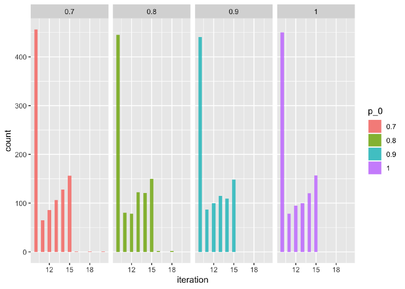
Figure 1: Number of rounds till the protocol finalizes, with $n=1000$, $a=0.75$, $b=0.85$, $m_{0}=\ell=5$, $k=20$, and $q=0.1$. Here, $p_{0}$ is the initial proportion of $1$-opinions among honest nodes; the round counts are on the horizontal axes, and on the vertical axes are numbers of nodes that have finalized on the $1$-opinion after that number of rounds.

It is interesting to observe that, in most cases, the protocol finalizes after the minimal number $m_{0}+\ell=10$ of rounds and the probability that it lasts for more than $20$ rounds seems to be very small.

Before starting with the proofs, let us mention that, for reader’s convenience, we provide the list of most important notations of this paper in Section 7 (page 7).

5 Proofs

We start with some preliminaries. Denote by $\mathcal{B}(m,p)$ the Binomial distribution with parameters $m\geq 1$ and $p\in[0,1]$. Let us recall the Hoeffding’s inequality [26]: if $\gamma\in(0,1)$ is a parameter and $S_{m}\sim\mathcal{B}(m,p)$ with $0<\gamma<p<1$, then

$${\mathbb{P}}\big{[}m^{-1}S_{m}\leq\gamma\big{]}\leq\exp\{-2m(p-\gamma)^{2}\};$$ (8)

the same estimate also holds for ${\mathbb{P}}[m^{-1}S_{m}\geq\gamma]$ in the case $0<p<\gamma<1$.

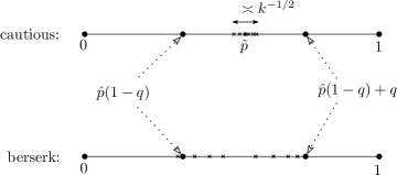
Figure 2: What cautious and berserk adversaries can achieve

To better understand the difference between cautious and berserk adversaries, look at Figure 2. Here, ${\hat{p}}$ is the initial proportion of $1$-opinions between the honest nodes, and the crosses mark the proportion of $1$-responses to the $k$ queries that the honest nodes obtain. The cautious adversary can choose any ${\tilde{p}}\in[{\hat{p}}(1-q),{\hat{p}}(1-q)+q]$ (by adjusting the opinions of his nodes appropriately, so that the overall proportion of $1$-opinions would be ${\tilde{p}}$), and then those crosses will be (mostly) concentrated in the interval of length of order $k^{-1/2}$ around ${\tilde{p}}$. On the other hand, the berserk adversary can cause the crosses to be distributed in any way on the whole interval $[{\hat{p}}(1-q),{\hat{p}}(1-q)+q]$, with some of them even going a bit out of it (on the distance of order $k^{-1/2}$ again).

Next, we need an auxiliary result on a likely outcome of a round in the case when the adversary cannot make the typical proportion of $1$-responses to be close to the decision threshold. Let $\eta(j)$ be the number of $1$-responses among $k$ queries that $j$th honest node receives; in general, the random variables $(\eta(j),j=1,\ldots,(1-q)n)$ are not independent, but they are conditionally independent given the adversary’s strategy. (Note that $\eta(j)\sim\mathcal{B}(k,{\tilde{p}})$ with some possibly random ${\tilde{p}}$ if the adversary is cautious, but the situation may be more complicated for a berserk one.) For a fixed $\lambda\in(0,1)$, define a random variable

$${\hat{p}}=\frac{1}{(1-q)n}\sum_{j=1}^{(1-q)n}{\mathbf{1}}{\{\eta(j)\geq\lambda k\}};$$

so that ${\hat{p}}$ is the new proportion of $1$-opinions among the honest nodes, given that the “decision threshold” equals $\lambda$. Then, the following result holds:

Lemma 5.1.

• Assume that, conditioned on any adversarial strategy, there are some positive $c$ and $\theta$ such that $\eta(j)$ is stochastically dominated by $\mathcal{B}(k,\lambda-c)$ for all $j=1,\ldots,(1-q)n$, and ${\mathbb{P}}[\mathcal{B}(k,\lambda-c)\geq\lambda k]\leq\theta$. Then, for any $v>0$

  $${\mathbb{P}}[{\hat{p}}>\theta+v]\leq e^{-2(1-q)nv^{2}}.$$ (9)

• Assume that, conditioned on any adversarial strategy, $\eta(j)$ stochastically dominates $\mathcal{B}(k,\lambda+c)$ for all $j=1,\ldots,(1-q)n$, and ${\mathbb{P}}[\mathcal{B}(k,\lambda+c)\leq\lambda k]\leq\theta$. Then, for any $v>0$

  $${\mathbb{P}}[{\hat{p}}<1-\theta-v]\leq e^{-2(1-q)nv^{2}}.$$ (10)

Proof.

For (i), we observe that $(1-q)n{\hat{p}}$ is stochastically dominated by $\mathcal{B}(n,\theta)$, and then (9) follows from (8). The proof of the part (ii) is completely analogous. ∎

Note that, by (8), ${\mathbb{P}}[\mathcal{B}(k,\lambda-c)\geq\lambda k]\leq e^{-2kc^{2}}$ (and the same holds for ${\mathbb{P}}[\mathcal{B}(k,\lambda+c)\leq\lambda k]$), so we will normally use Lemma 5.1 with $\theta=e^{-2kc^{2}}$.

Another elementary fact we need is

Lemma 5.2.

Let $(\xi_{m}^{(j)},m\geq 1),j=1,\ldots,N$ be $N$ sequences of independent Bernoulli trials with success probability $h\in(0,1)$. For $j=1,\ldots,N$ define

$$\tau^{(1)}_{j}=\min\big{\{}m\geq\ell:\xi_{m}^{(j)}=\xi_{m-1}^{(j)}=\ldots=\xi_{m-\ell+1}^{(j)}=1\big{\}}$$

and

$$\tau^{(0)}_{j}=\min\big{\{}m\geq\ell:\xi_{m}^{(j)}=\xi_{m-1}^{(j)}=\ldots=\xi_{m-\ell+1}^{(j)}=0\big{\}}$$

to be the first moments when runs of $\ell$ ones (respectively, zeros) are observed in $j$th sequence. Then, for all $u\in{\mathbb{N}}$,

$${\mathbb{P}}[\tau^{(1)}_{j}\leq\ell u,\tau^{(1)}_{j}<\tau^{(0)}_{j}]\geq 1-(1-h^{\ell})^{u}-\Big{(}\frac{1-h}{h}\Big{)}^{\ell-1}$$ (11)

for all $j=1,\ldots,N$, and

$${\mathbb{P}}[\tau^{(1)}_{j}\leq\ell u,\tau^{(1)}_{j}<\tau^{(0)}_{j},\forall j=1,\ldots,N]\geq 1-N\Big{(}(1-h^{\ell})^{u}+\Big{(}\frac{1-h}{h}\Big{)}^{\ell-1}\Big{)}.$$ (12)

Proof.

First, it is clear that

$${\mathbb{P}}[\tau^{(1)}_{j}\leq\ell u]\geq 1-(1-h^{\ell})^{u}$$ (13)

(divide the time interval $[1,\ell u]$ into $u$ subintervals of length $\ell$ and note that each of these subintervals is all-$1$ with probability $h^{\ell}$). Then, the following is an easy exercise on computing probabilities via conditioning (for the sake of completeness, we prove this fact in the Appendix):

$${\mathbb{P}}[\tau^{(1)}_{j}<\tau^{(0)}_{j}]=1-\frac{(1-h)^{\ell-1}(1-h^{\ell})}{h^{\ell-1}+(1-h)^{\ell-1}-(h(1-h))^{\ell-1}}.$$ (14)

Observe that (14) implies that (since $1-h^{\ell}\leq 1$ and $(1-h)^{\ell-1}-(h(1-h))^{\ell-1}\geq 0$)

$${\mathbb{P}}[\tau^{(1)}_{j}<\tau^{(0)}_{j}]\geq 1-\Big{(}\frac{1-h}{h}\Big{)}^{\ell-1},$$

and so, using the above together with (13) and the union bound, we obtain (11). The relation (12) is then a direct consequence of (11) (again, with the union bound). ∎

To prove our main results, we need some additional notation. Let $\varrho(j)$ be the round when the $j$th (honest) node finalizes its opinion. Denote

$$R_{m}=\{j:\varrho(j)\leq m\}$$

to be the subset of honest nodes that finalized their opinions by round $m$. Let also ${\hat{\xi}}_{m}(j)$ be the opinion of $j$th node after the $m$th round and

$${\hat{p}}_{m}=\frac{1}{(1-q)n}\sum_{j=1}^{(1-q)n}{\hat{\xi}}_{m}(j)$$ (15)

be the proportion of $1$-opinions among the honest nodes after the $m$th round in the original system.

Proof of Theorem 4.1..

Let us define the random variable

$$\Psi=\min\Big{\{}m\geq 1:{\hat{p}}_{m}\leq\frac{\beta-q}{2(1-q)}\text{ or }{\hat{p}}_{m}\geq 1-\frac{\beta-q}{2(1-q)}\Big{\}}$$ (16)

to be the round after which the proportion of $1$-opinions among the honest nodes either becomes “too small”, or “too large”. We now need the following fact:

Lemma 5.3.

For all $s\leq m_{0}+\ell$, it holds that (recall (3) and (4))

$${\mathbb{P}}[\Psi>s]\leq\begin{cases}\big{(}\psi_{cau}(n,k)\big{)}^{s-1},&\text{for cautious adversary},\\ \big{(}\psi_{ber}(n,k)\big{)}^{s-1},\vphantom{\int\limits^{B}}&\text{for berserk adversary}.\end{cases}$$ (17)

Proof.

Observe that $s\leq m_{0}+\ell$ implies that a node cannot finalize its opinion before round $s$. Consider first the case of a cautious adversary. Abbreviate (for this proof) $\mu=\frac{\beta-q}{4(1-q)}$. Let $m\geq 2$ and observe that, for any fixed $h\in[0,1]$ we have (recall that $X_{m}\sim U[\beta,1-\beta]$)

$${\mathbb{P}}\big{[}e^{-2k(X_{m}-h)^{2}}\geq\mu\big{]} ={\mathbb{P}}\Big{[}(X_{m}-h)^{2}\leq\frac{\ln\mu^{-1}}{2k}\Big{]}$$

$$={\mathbb{P}}\Big{[}h-\sqrt{\frac{\ln\mu^{-1}}{2k}}\leq X_{m}\leq h+\sqrt{\frac{\ln\mu^{-1}}{2k}}\Big{]}$$

$$\leq(1-2\beta)^{-1}\sqrt{\frac{2\ln\mu^{-1}}{k}}.$$ (18)

Now, assume that ${\tilde{p}}_{m-1}=h$. Under this, using (8) and (18), we obtain by conditioning on the value of $X_{m}$

$${\mathbb{P}}[{\hat{p}}_{m}\in(2\mu,1-2\mu)] ={\mathbb{E}}{\mathbb{P}}[{\hat{p}}_{m}\in(2\mu,1-2\mu)\mid X_{m}]$$

$$={\mathbb{E}}\big{(}{\mathbb{P}}[{\hat{p}}_{m}\in(2\mu,1-2\mu)\mid X_{m}]{\mathbf{1}}{\{e^{-2k(X_{m}-h)^{2}}<\mu\}}$$

$$\qquad+{\mathbb{P}}[{\hat{p}}_{m}\in(2\mu,1-2\mu)\mid X_{m}]{\mathbf{1}}{\{e^{-2k(X_{m}-h)^{2}}\geq\mu\}}\big{)}$$

$$\leq{\mathbb{E}}\big{(}{\mathbb{P}}[{\hat{p}}_{m}>2\mu\mid X_{m}]{\mathbf{1}}{\{e^{-2k(X_{m}-h)^{2}}<\mu,h<X_{m}\}}$$

$$\qquad+{\mathbb{P}}[{\hat{p}}_{m}<1-2\mu\mid X_{m}]{\mathbf{1}}{\{e^{-2k(X_{m}-h)^{2}}<\mu,h>X_{m}\}}$$

$$\qquad+{\mathbf{1}}{\{e^{-2k(X_{m}-h)^{2}}\geq\mu\}}\big{)}$$

$$\leq 2{\mathbb{P}}\big{[}((1-q)n)^{-1}{\cal B}((1-q)n,e^{-2k(1-\mu)})<1-2\mu\big{]}$$

$$\qquad+{\mathbb{P}}[e^{-2k(X_{m}-h)^{2}}\geq\mu]$$

$$\leq\psi_{cau}(n,k),$$ (19)

recall (3). This implies the first comparison in (17).

For a berserk adversary, the calculation is quite analogous (recall Figure 2), so we omit it. ∎

Next, we need a result that shows that if one of the opinions has already reached a supermajority, then this situation is likely to be preserved.

Figure 3: Transition from ${\hat{p}}_{m}$ to ${\hat{p}}_{m+1}$: after $m$th round, being ${\hat{p}}_{m}\leq\frac{\beta-q}{2(1-q)}$, the adversary may “grow” the proportion of $1$s to ${\hat{p}}_{m}(1-q)+q\leq\frac{\beta+q}{2}$. Then, since the difference between that and “the least possible threshold” $\beta$ is at least $\frac{\beta-q}{2}$, the probability that an undecided node would have opinion $1$ in the next round is at most $e^{-\frac{1}{2}k(\beta-q)^{2}}$. Then, with overwhelming probability ${\hat{p}}_{m+1}$ will be at most $\frac{\beta-q}{2(1-q)}$, and so it goes.

Lemma 5.4.

Let $m\geq 2$; in the following, $A$ will denote a subset of $\{1,\ldots,(1-q)n\}$.

• Let $G_{0}$ be the event that ${\hat{p}}_{m}\leq\frac{\beta-q}{2(1-q)}$, $R_{m-1}=A$, and ${\hat{\xi}}_{m-1}(j)=0$ for all $j\in A$. Then

  $${\mathbb{P}}\Big{[}{\hat{p}}_{m+1}\leq\frac{\beta-q}{2(1-q)}\;\big{|}\;G_{0}\Big{]}\geq 1-e^{-2(1-q)n\varphi_{\beta,q,k}^{2}}.$$ (20)

• Let $G_{1}$ be the event that ${\hat{p}}_{m}\geq 1-\frac{\beta-q}{2(1-q)}$, $R_{m-1}=A$, and ${\hat{\xi}}_{m-1}(j)=1$ for all $j\in A$. Then

  $${\mathbb{P}}\Big{[}{\hat{p}}_{m+1}\geq 1-\frac{\beta-q}{2(1-q)}\;\big{|}\;G_{1}\Big{]}\geq 1-e^{-2(1-q)n\varphi_{\beta,q,k}^{2}}.$$ (21)

Proof.

We prove only part (i), the proof of the other part is completely analogous. Now, look at Figure 3: essentially, this is a direct consequence of Lemma 5.1 with $\theta=e^{-2k(\frac{\beta-q}{2})^{2}}=e^{-\frac{1}{2}k(\beta-q)^{2}}$ and $v=\varphi_{\beta,q,k}$. Observe also that, if some honest nodes already decided on $0$ definitely, it holds that $(1-q)n{\hat{p}}_{m+1}$ is stochastically dominated by $\mathcal{B}\big{(}(1-q)n,e^{-\frac{1}{2}k(\beta-q)^{2}}\big{)}$. ∎

Now, we are able to conclude the proof of Theorem 4.1. Let us introduce the random variable

$$Z=\begin{cases}\min\Big{\{}m>\Psi:{\hat{p}}_{m}>\frac{\beta-q}{2(1-q)}\Big{\}}&\text{on }{\hat{p}}_{\Psi}\leq\frac{\beta-q}{2(1-q)},\\ \min\Big{\{}m>\Psi:{\hat{p}}_{m}<1-\frac{\beta-q}{2(1-q)}\Big{\}}\vphantom{\int\limits^{A^{A}}}&\text{on }{\hat{p}}_{\Psi}\geq 1-\frac{\beta-q}{2(1-q)}\end{cases}$$ (22)

to be the first moment after $\Psi$ when the honest nodes’ opinion has drifted away from supermajority. Denote also

$${\hat{\tau}}^{(1)}_{j}=\min\big{\{}m\geq m_{0}+\ell:{\hat{\xi}}_{m}^{(j)}={\hat{\xi}}_{m-1}^{(j)}=\ldots={\hat{\xi}}_{m-\ell+1}^{(j)}=1\big{\}}$$

and

$${\hat{\tau}}^{(0)}_{j}=\min\big{\{}m\geq m_{0}+\ell:{\hat{\xi}}_{m}^{(j)}={\hat{\xi}}_{m-1}^{(j)}=\ldots={\hat{\xi}}_{m-\ell+1}^{(j)}=0\big{\}}.$$

Next, observe that

$$(H_{0}\cup H_{1})\cap\{\mathcal{N}\leq m_{0}+\ell u\}\subset D_{1}\cap D_{2}\cap D_{3},$$

where

$$D_{1} =\{\Psi\leq m_{0}\},$$

$$D_{2} =\{Z\geq m_{0}+\ell u\},$$

$$D_{3} =\big{\{}\text{there is }i\in\{0,1\}\text{ such that }{\hat{\tau}}^{(i)}_{j}\leq m_{0}+\ell u,{\hat{\tau}}^{(i)}_{j}<{\hat{\tau}}^{(1-i)}_{j}$$

$$\qquad\qquad\qquad\qquad\qquad\qquad\qquad\qquad\text{ for all }j=1,\ldots,(1-q)n\big{\}}.$$

To obtain the estimates (5) and (6), it is enough to note that the lower bounds on, respectively, ${\mathbb{P}}[D_{1}]$, ${\mathbb{P}}[D_{2}]$, and ${\mathbb{P}}[D_{3}]$, follow from, respectively, Lemma 5.3, Lemma 5.4, and Lemma 5.2 (and also the union bound). ∎

Proof of Theorem 4.4..

We prove only the part (i); the proof of the other part is completely analogous. In fact, to obtain the proof it is enough to observe that, if $a-{\hat{p}}_{0}(1-q)-q>0$ and $e^{-2k(a-{\hat{p}}_{0}(1-q)-q)^{2}}\leq\frac{\beta-q}{4(1-q)}$, then, by (8), with probability at least $1-\exp\big{(}-\tfrac{1}{8}n\tfrac{(\beta-q)^{2}}{4(1-q)}\big{)}$ it happens that ${\hat{p}}_{1}\leq\frac{\beta-q}{2(1-q)}$ (so, in particular, $\Psi=1$); next, the same argument as in the proof of Theorem 4.1 does the work. ∎

6 Further generalizations

In this section we argue that our protocol is robust, that is, it is possible to adapt it in such a way that it is able to work well in more “practical” situations. Specifically, observe that nodes may not always respond queries, and the adversarial nodes sometimes may do so deliberately. The protocol described in Section 3 is not designed to handle this, so it needs to be amended. There are at least two natural ways to deal with this situation:

• let each node to take the decision based on the responses that it effectively received (i.e., instead of $k^{-1}\eta_{m}(j)$ use $\eta_{m}(j)/\zeta_{m}(j)$, where $\zeta_{m}(j)$ is the number of responses that the $j$th node received in the $m$th round);

• each node queries more than $k$ nodes, say, $2k$ or more; since whp the number of responses received will be at least $k$ (for definiteness, let us assume that the probability that a query is left unresponded is less than $\frac{1}{2}$), the node then keeps exactly $k$ responses and discards the rest;

and it is of course also possible to combine them. The practical difference between these two options is probably not so big at least in the case of reasonably large values of $k$ (because then the proportions of $1$s in the responses should be roughly the same in most cases due to the Law of Large Numbers); for the sake of formulating the results in a more clean way, let us assume that a node simply issues queries sequentially until getting exactly $k$ responses.

Now, we define the notion of a semi-cautious adversary: every node it controls will not give contradicting responses (i.e., $0$ to one node and $1$ to another node in the same round) but can sometimes remain silent; since it does not make sense for a node to remain silent altogether in a given round (that would just reduce the fraction of the adversarial nodes in the network), there are two possible adversarial node behaviours:

• a node answers “$0$” to some queries and does not answer other queries;

• a node answers “$1$” to some queries and does not answer other queries.

Here is the result we have for a semi-cautious adversary:

Theorem 6.1.

If the adversary is semi-cautious, assume that $\frac{1}{2-q}-\beta+\sqrt{2k^{-1}\ln\tfrac{4(1-q)}{\beta-q}}<1-2\beta$. Then, for any adversarial strategy, we have

$${\mathbb{P}}\big{[}(H_{0}\cup H_{1})\cap\{\mathcal{N}\leq m_{0}+\ell u\}\big{]} \geq 1-\big{(}\psi_{semi}(n,k)\big{)}^{m_{0}}-W(n,k,m_{0},\ell,u),$$ (23)

where

$$\psi_{semi}(n,k)=2\exp\big{(}-\tfrac{1}{8}n\tfrac{(\beta-q)^{2}}{4(1-q)}\big{)}+\frac{\frac{1}{2-q}-\beta+\sqrt{2k^{-1}\ln\tfrac{4(1-q)}{\beta-q}}}{1-2\beta}.$$ (24)

In this situation, the fact corresponding to Corollary 4.2 will be the following (in particular, note the new “security threshold” $\phi^{-2}\in(\frac{1}{3},\frac{1}{2})$ that we obtain here):

Corollary 6.2.

For a semi-cautious adversary, we need that $\frac{1}{2-q}-\beta<1-2\beta$, or, equivalently, $q<2-\frac{1}{1-\beta}$ (it is only in this case that we will be able to find large enough $k$ such that the hypothesis of Theorem 6.1 is satisfied). Since we also still need that $q<\beta$, solving $\beta=2-\frac{1}{1-\beta}$, we obtain that $q$ must be less than $\frac{3-\sqrt{5}}{2}=\frac{1}{1+\phi}=\phi^{-2}\approx 0.38$, where $\phi=\frac{1+\sqrt{5}}{2}$ is the Golden Ratio. Then, as before, it is straightforward to show that, for a semi-cautious adversary, for any $q<\frac{1}{1+\phi}$ and all large enough $n$ we are able to adjust the parameters $k,\beta,m_{0},\ell$ in such a way that the protocol works whp (in particular, a $\beta$-value sufficiently close to $\frac{1}{1+\phi}$ would work).

Proof of Theorem 6.1.

As observed before, an “always-silent” strategy is not interesting for an adversarial node, since this will, in practice, only reduce their quantity. Now, assume that, for some $\gamma\in[0,1]$,

• $\gamma qn$ adversarial nodes reply “$0$” or remain silent;

• $(1-\gamma)qn$ adversarial nodes reply “$1$” or remain silent.

Then, if the adversary wants to decrease a honest node’s confidence in the $1$-opinion, those nodes who may answer “$1$” will remain silent, and so with probability $\frac{1-q}{1-q+\gamma q}$ the response will be obtained from a honest node, while with probability $\frac{\gamma q}{1-q+\gamma q}$ the response will be obtained from an adversarial node. This gives

$${\hat{p}}\frac{1-q}{1-q+\gamma q}=\frac{{\hat{p}}(1-q)}{1-(1-\gamma)q}$$

as the “lower limit” for the (expected) proportion of $1$s in the queries. Analogously, if the adversary wants to increase an honest node’s confidence in the $1$-opinion those nodes who may answer “$0$” will remain silent, and so with probability $\frac{1-q}{1-q+(1-\gamma)q}$ the response will be obtained from a honest node, while with probability $\frac{(1-\gamma)q}{1-q+(1-\gamma)q}$ the response will be obtained from an adversarial node. This gives

$${\hat{p}}\frac{1-q}{1-q+(1-\gamma)q}+\frac{(1-\gamma)q}{1-q+(1-\gamma)q}=\frac{{\hat{p}}(1-q)+(1-\gamma)q}{1-\gamma q}$$

as the corresponding “upper limit”. So, analogously to Figure 2, the semi-cautious adversary can achieve the “crosses” to be distributed on the interval

$$\mathcal{I}_{\gamma}:=\Big{[}\frac{{\hat{p}}(1-q)}{1-(1-\gamma)q},\frac{{\hat{p}}(1-q)+(1-\gamma)q}{1-\gamma q}\Big{]}$$ (25)

in any way. Now, it is elementary to see that both endpoints of the above interval decrease when $\gamma$ increases; if we want to make it symmetric (around $\frac{1}{2}$), we need to solve

$$\frac{{\hat{p}}(1-q)}{1-(1-\gamma)q}=1-\frac{{\hat{p}}(1-q)+(1-\gamma)q}{1-\gamma q},$$

or, equivalently

$$\frac{{\hat{p}}}{1-(1-\gamma)q}=\frac{1-{\hat{p}}}{1-\gamma q}$$

for $\gamma$. This gives the solution $\gamma^{*}=q^{-1}(2{\hat{p}}-1)+(1-{\hat{p}})$. After substituting $\gamma^{*}$ to (25), the symmetrized interval becomes

$$\mathcal{I}_{\gamma^{*}}=\Big{[}\frac{1-q}{2-q},\frac{1}{2-q}\Big{]}$$

(somewhat unexpectedly, because it doesn’t depend on ${\hat{p}}$ anymore).

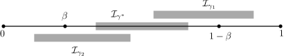
Figure 4: The “intervals of control” of a semi-cautious adversary, for $\gamma_{1}<\gamma^{*}<\gamma_{2}$

It is actually worth noting that $\gamma^{*}$ does not necessarily belong to $[0,1]$ (so it is not always possible to make this interval symmetric), but it does not pose a problem due to the following. Look at Figure 4: due to the monotonicity,

$$\max_{\gamma\in[0,1]}\big{|}[\beta,1-\beta]\cap\mathcal{I}_{\gamma}\big{|}\leq\frac{1}{2-q}-\beta;$$ (26)

indeed, for all $\gamma$ we see that either the interval $[\beta,\frac{1-q}{2-q})$ or the interval $(\frac{1}{2-q},1-\beta]$ is a subset of $[\beta,1-\beta]\setminus\mathcal{I}_{\gamma}$.

This essentially takes care of the argument in the proof of Lemma 5.3 (since we now understand what is the minimal length of the interval that the adversary cannot control), and the rest of the proof is completely analogous to that of Theorem 4.1: indeed, as observed before, the adversary loses control after the random time $\Psi$. ∎

We also observe that Theorem 4.4 remains valid also for a semi-cautious adversary.

Next, let us discuss what do we really need from the (decentralized) random number generator. In fact, it is not so much: we need that, regardless of the past, with probability at least $\theta$ (where $\theta>0$ is a fixed parameter) the next outcome is a uniform random variable which is “unpredictable” for the adversary; this random number is seen by at least (1-$\delta$) proportion of honest nodes, where $\delta$ is reasonably small. What we can prove in such a situation depends on what the remaining $\delta(1-q)n$ honest nodes use as their decision thresholds: they can use some “second candidate” (in case there is an alternative source of common randomness), or they can choose their thresholds independently and randomly, etc. Each of such situations would need to be treated separately, which is certainly doable, but left out of this paper. Let us note, though, that the “worst-case” assumption is that the adversary can “feed” the (fake) decision thresholds to those $\delta(1-q)n$ honest nodes. This would effectively mean that these nodes would behave as cautious adversaries in the next round (which matters if the random time $\Psi$ did not yet occur). Therefore, for the sake of obtaining bounds like (5)–(6) and (23) we can simply pretend that the value of $q$ is increased by $\delta$.

Now, assuming that $\delta=0$, it is easy to figure out how this will affect our results: indeed, in our proofs, all random thresholds matter only until $\Psi$. It is then straightforward to obtain the following fact:

Proposition 6.3.

Assume the above on the random number generation (with $\theta\in(0,1)$ and $\delta=0$). Then, the estimates (5)–(6) and (23) remain valid with $1-\theta+\theta\psi_{*}(n,k)$ on the place of $\psi_{*}(n,k)$ (with $*\in\{\text{cau},\text{ber},\text{semi}\}$).

In view of the above result, let us stress that one of the main ideas of this paper is: we use a “rather weak” consensus (on the random numbers, as above) to obtain a “strong” consensus on the value of a bit (i.e., validity of a transaction). Also, let us observe that a partial control of the random numbers does not give access to a lot of power (in the worst case the adversary would delay the consensus a bit, but that is all), so there is not much need to be restrictive on the degree of decentralization for that part: a smaller subcommittee can take care of the random numbers’ generation, and some VDF-based random number generation scheme (such as [21]) may be used to further prevent this subcommittee from leaking the numbers before the due time).

7 Notations used in this paper

Here, for reader’s convenience, we provide a list of most important notations used in the paper.

• $n\in{\mathbb{N}}$ is the total number of nodes in the system, $k\in{\mathbb{N}}$ is the number of queries each node makes in one round, $q\in[0,1)$ is the proportion of adversarial nodes;

• $1/2<a\leq b<1$ are the threshold limits in the first round, $\beta\in(0,1/2)$ is the threshold limit parameter in the subsequent rounds;

• in the same round, a cautious adversarial node always responds the queries in the same way, a berserk one can give any responses (including not responding at all), and a semi-cautious one may ignore some of the queries but has to respond the others in the same way;

• for our protocol to work, for all cases we need to assume that $q<\beta$; additionally, we also need to assume that $q<1-2\beta$ for berserk adversary and $q<2-\frac{1}{1-\beta}$ for semi-cautious adversary;

• $m_{0}\in{\mathbb{N}}$, the cooling-off period, $\ell\in{\mathbb{N}}$ is the number of consecutive rounds with the same opinion after which it becomes final;

• $\eta_{m}(j)\in\{1,\ldots,k\}$ is the number of $1$-opinions that $j$th node receives in $m$th round;

• $U[s,r]$ is the Uniform probability distribution of the interval $[s,r]$ and $\mathcal{B}(m,p)$ is the Binomial distribution with parameters $m\geq 1$ and $p\in[0,1]$;

• $W(\cdot,\cdot,\cdot,\cdot,\cdot)$ is defined in (2), $\psi_{cau}(\cdot,\cdot)$ and $\psi_{ber}(\cdot,\cdot)$ are defined in (3)–(4), and $\psi_{semi}(\cdot,\cdot)$ is defined in (24);

• $H_{0}\cap H_{1}$ is the “consensus event” (i.e., either all honest nodes finalize on $0$ or all honest nodes finalize on $1$);

• $\mathcal{N}$ is the number of rounds until all honest nodes finalize their opinions;

• ${\hat{p}}_{0}$ is the initial proportion of $1$-opinions among the honest nodes;

• ${\hat{p}}_{m}$ is the proportion of $1$-opinions among the honest nodes after the $m$th round;

• $R_{m}\subset\{1,\ldots,n\}$ is the set of honest nodes that finalized their opinions by round $m$;

• $\Psi\in{\mathbb{N}}$ is the (random) moment when the adversary “looses control” (formally defined in (16)).

8 Conclusions and Future Work

In this paper we described a consensus protocol which is able to withstand a substantial proportion of Byzantine nodes, and obtained some explicit estimates on its safety and liveness. A special feature of our protocol is that it uses a sequence of random numbers (produced by some external source or by the nodes themselves) in order to have a “randomly moving decision threshold” which quickly defeats the adversary’s attempts to mess with the consensus. It is also worth noting that the “quality” of those random numbers is not critically important – only the estimates on $\Psi$ (Lemma 5.3) will be affected in a non-drastic way. In particular, one can permit that the random numbers might be biased, or even that the adversary might get control of these numbers from time to time. Also, it is clear from the proofs that there is no need for the honest nodes to achieve consensus on the actual values of these random numbers: if some (not very large) proportion of honest nodes does not see the same number as the others, this will not cause problems. All this is due to the fact that, when the proportion of $1$-opinions among the honest nodes becomes “too small” or “too large” (i.e., less than $\frac{\beta-q}{2(1-q)}$ or greater than $1-\frac{\beta-q}{2(1-q)}$ in our proofs), the adversary does not have any control anymore.

As mentioned above, this paper primarily contains a rigorous analysis of the simplest version of the protocol. It is of course tempting to consider other versions, in particular, where the neighborhood relation between nodes is not that of a complete graph. However, as is frequently the case, introducing a nontrivial graph structure makes the problem hardly tractable in a purely analytic way, which means that it has to be approached via simulations. For that approach, we refer to the paper [27], which can be considered as a complementary work to the present one (note that simulations also permit one to obtain better estimates the failure probabilities since, as noted above, the estimates (5) and (6) of the present paper are usually not quite sharp).

Also, when considering the behavior of the adversary nodes, a number of “worst-case” assumptions were made (notably, that all the adversarial nodes are controlled by a single entity and that the adversary is omniscient). Again, analysing a system with independent adversaries with possibly incomplete information is an interesting but analytically difficult program; in this case the simulations approach seems to be more adequate as well.

We need to comment on anti-Sybil measure in practical implementations: indeed, it would be quite unfortunate if the adversary is able to deploy an excessively large number of nodes, thus inflating the value of $q$. One of the possible approaches is using a variant of Proof-of-Stake; with it, when querying, one needs to choose the node proportionally to its weight (stake). This is partly the subject of an ongoing research effort [28].

Appendix A Runs of zeros and ones in Bernoulli trials

Here we prove a simple fact about runs of zeros and ones in a sequence of Bernoulli trials, which will imply (14). Namely, let $\xi_{1},\xi_{2},\xi_{3},\ldots$ be i.i.d. random variables with ${\mathbb{P}}[\xi_{i}=1]=1-{\mathbb{P}}[\xi_{i}=0]=h$, and let, for $r,s\in{\mathbb{N}}$

$$\tau=\min\{m\geq r:\xi_{m}=\xi_{m-1}=\ldots=\xi_{m-r+1}=1\}$$

and

$$\sigma=\min\{m\geq s:\xi_{m}=\xi_{m-1}=\ldots=\xi_{m-s+1}=0\}$$

to be the first moments when we see runs of $r$ ones (respectively, $s$ zeros).

Proposition A.1.

It holds that

$${\mathbb{P}}[\tau<\sigma]=\frac{h^{r-1}(1-(1-h)^{s})}{h^{r-1}+(1-h)^{s-1}-h^{r-1}(1-h)^{s-1}}.$$ (27)

Proof.

To prove (27), we use conditioning. Abbreviate $p_{0}={\mathbb{P}}[\tau<\sigma\mid\xi_{1}=0]$ and $p_{1}={\mathbb{P}}[\tau<\sigma\mid\xi_{1}=1]$. Then, conditioning on the number of consecutive zeros in the beginning, we write

$$p_{0}=\sum_{j=1}^{s-1}(1-h)^{j-1}hp_{1}=(1-(1-h)^{s-1})p_{1},$$ (28)

and, conditioning on the number of consecutive ones in the beginning, we obtain that

$$p_{1}=\sum_{j=1}^{r-1}h^{j-1}(1-h)p_{0}+\sum_{j=r}^{\infty}h^{j-1}(1-h)\times 1=(1-h^{r-1})p_{0}+h^{r-1}.$$ (29)

Solving (28)–(29) for $p_{0,1}$ yields

$$p_{0} =\frac{h^{r-1}(1-(1-h)^{s-1})}{h^{r-1}+(1-h)^{s-1}-h^{r-1}(1-h)^{s-1}},$$

$$p_{1} =\frac{h^{r-1}}{h^{r-1}+(1-h)^{s-1}-h^{r-1}(1-h)^{s-1}},$$

and we then obtain (27) by using the obvious relation ${\mathbb{P}}[\tau<\sigma]=(1-h)p_{0}+hp_{1}$. ∎

References

- [1] Z. Zheng, S. Xie, H. Dai, X. Chen, and H. Wang, “An overview of blockchain technology: Architecture, consensus, and future trends,” in 2017 IEEE International Congress on Big Data (BigData Congress). IEEE, 2017, pp. 557–564.
- [2] M. K. Aguilera and S. Toueg, “The correctness proof of Ben-Or’s randomized consensus algorithm,” Distributed Computing, vol. 25, no. 5, pp. 371–381, 2012.
- [3] M. Ben-Or, “Another advantage of free choice: Completely asynchronous agreement protocols (extended abstract),” in Proceedings of the 2nd ACM Annual Symposium on Principles of Distributed Computing, Montreal, Quebec, 1983, pp. 27–30.
- [4] G. Bracha, “Asynchronous Byzantine agreement protocols,” Information and Computation, vol. 75, no. 2, pp. 130–143, 1987.
- [5] P. Feldman and S. Micali, “An optimal probabilistic algorithm for synchronous Byzantine agreement,” in International Colloquium on Automata, Languages, and Programming. Springer, 1989, pp. 341–378.
- [6] R. Friedman, A. Mostefaoui, and M. Raynal, “Simple and efficient oracle-based consensus protocols for asynchronous Byzantine systems,” IEEE Transactions on Dependable and Secure Computing, vol. 2, no. 1, pp. 46–56, 2005.
- [7] M. O. Rabin, “Randomized Byzantine generals,” in 24th Annual Symposium on Foundations of Computer Science (sfcs 1983). IEEE, 1983, pp. 403–409.
- [8] J. Liu, W. Li, G. O. Karame, and N. Asokan, “Scalable Byzantine consensus via hardware-assisted secret sharing,” IEEE Transactions on Computers, vol. 68, no. 1, pp. 139–151, 2018.
- [9] T. Crain, V. Gramoli, M. Larrea, and M. Raynal, “Dbft: Efficient leaderless Byzantine consensus and its application to blockchains,” in 2018 IEEE 17th International Symposium on Network Computing and Applications (NCA). IEEE, 2018, pp. 1–8.
- [10] A. Miller, Y. Xia, K. Croman, E. Shi, and D. Song, “The honey badger of bft protocols,” in Proceedings of the 2016 ACM SIGSAC Conference on Computer and Communications Security. ACM, 2016, pp. 31–42.
- [11] R. A. Holley, T. M. Liggett et al., “Ergodic theorems for weakly interacting infinite systems and the voter model,” The annals of probability, vol. 3, no. 4, pp. 643–663, 1975.
- [12] P. Clifford and A. Sudbury, “A model for spatial conflict,” Biometrika, vol. 60, no. 3, pp. 581–588, 1973. [Online]. Available: http://www.jstor.org/stable/2335008
- [13] L. Becchetti, A. Clementi, E. Natale, F. Pasquale, and L. Trevisan, “Stabilizing consensus with many opinions,” in Proceedings of the twenty-seventh annual ACM-SIAM symposium on Discrete algorithms. SIAM, 2016, pp. 620–635.
- [14] C. Cooper, R. Elsässer, and T. Radzik, “The power of two choices in distributed voting,” in International Colloquium on Automata, Languages, and Programming. Springer, 2014, pp. 435–446.
- [15] C. Cooper, R. Elsässer, T. Radzik, N. Rivera, and T. Shiraga, “Fast consensus for voting on general expander graphs,” in International Symposium on Distributed Computing. Springer, 2015, pp. 248–262.
- [16] R. Elsässer, T. Friedetzky, D. Kaaser, F. Mallmann-Trenn, and H. Trinker, “Rapid asynchronous plurality consensus,” arXiv preprint arXiv:1602.04667, 2016.
- [17] G. Fanti, N. Holden, Y. Peres, and G. Ranade, “Communication cost of consensus for nodes with limited memory,” arXiv preprint arXiv:1901.01665, 2019.
- [18] J. Cruise and A. Ganesh, “Probabilistic consensus via polling and majority rules,” Queueing Syst. Theory Appl., vol. 78, no. 2, pp. 99–120, Oct. 2014. [Online]. Available: http://dx.doi.org/10.1007/s11134-014-9397-7
- [19] Y. Aumann and Y. Lindell, “Security against covert adversaries: Efficient protocols for realistic adversaries,” in Theory of Cryptography Conference. Springer, 2007, pp. 137–156.
- [20] I. Cascudo and B. David, “Scrape: Scalable randomness attested by public entities,” in International Conference on Applied Cryptography and Network Security. Springer, 2017, pp. 537–556.
- [21] A. K. Lenstra and B. Wesolowski, “Trustworthy public randomness with sloth, unicorn, and trx,” International Journal of Applied Cryptography, vol. 3, no. 4, pp. 330–343, 2017. [Online]. Available: https://www.inderscienceonline.com/doi/abs/10.1504/IJACT.2017.089354
- [22] S. Popov, “On a decentralized trustless pseudo-random number generation algorithm,” Journal of Mathematical Cryptology, vol. 11, no. 1, pp. 37–43, 2017.
- [23] P. Schindler, A. Judmayer, N. Stifter, and E. Weippl, “Hydrand: Practical continuous distributed randomness,” Cryptology ePrint Archive, Report 2018/319, 2018, https://eprint.iacr.org/2018/319.
- [24] E. Syta, P. Jovanovic, E. K. Kogias, N. Gailly, L. Gasser, I. Khoffi, M. J. Fischer, and B. Ford, “Scalable bias-resistant distributed randomness,” in 2017 IEEE Symposium on Security and Privacy (SP). IEEE, 2017, pp. 444–460.
- [25] T. Rocket, M. Yin, K. Sekniqi, R. van Renesse, and E. G. Sirer, “Scalable and probabilistic leaderless bft consensus through metastability,” 2019.
- [26] W. Hoeffding, “Probability inequalities for sums of bounded random variables,” in The Collected Works of Wassily Hoeffding. Springer, 1994, pp. 409–426.
- [27] A. Capossele, S. Müller, and A. Penzkofer, “Robustness and efficiency of leaderless probabilistic consensus protocols within byzantine infrastructures,” 2019.
- [28] S. Müller, A. Penzkofer, B. Kuśmierz, D. Camargo, and W. J. Buchanan, “Fast Probabilistic Consensus with Weighted Votes (work in progress),” 2020.
Acknowledgments
The author thanks Hans Moog, Sebastian Müller, Luigi Vigneri, and Wolfgang Welz for valuable comments and suggestions and also for providing some simulations of the model.