Extreme Multi-Label Legal Text Classification:
A case study in EU Legislation

Abstract

We consider the task of Extreme Multi-Label Text Classification (xmtc) in the legal domain. We release a new dataset of 57k legislative documents from eur-lex, the European Union’s public document database, annotated with concepts from eurovoc, a multidisciplinary thesaurus. The dataset is substantially larger than previous eur-lex datasets and suitable for xmtc, few-shot and zero-shot learning. Experimenting with several neural classifiers, we show that bigrus with self-attention outperform the current multi-label state-of-the-art methods, which employ label-wise attention. Replacing cnns with bigrus in label-wise attention networks leads to the best overall performance.

1 Introduction

Extreme multi-label text classification (xmtc), is the task of tagging documents with relevant labels from an extremely large label set, typically containing thousands of labels (classes). Applications include building web directories Partalas et al. (2015), labeling scientific publications with concepts from ontologies Tsatsaronis et al. (2015), product categorization McAuley and Leskovec (2013), categorizing medical examinations Mullenbach et al. (2018); Rios and Kavuluru (2018b), and indexing legal documents Mencia and Fürnkranz (2007). We focus on legal text processing, an emerging nlp field with many applications Nallapati and Manning (2008); Aletras et al. (2016); Chalkidis et al. (2017), but limited publicly available resources.

We release a new dataset, named eurlex57k, including 57,000 English documents of eu legislation from the eur-lex portal. All documents have been tagged with concepts from the European Vocabulary (eurovoc), maintained by the Publications Office of the European Union. Although eurovoc contains more than 7,000 concepts, most of them are rarely used in practice. Consequently, they are under-represented in eurlex57k, making the dataset also appropriate for few-shot and zero-shot learning.

Experimenting on eurlex57k, we explore the use of various rnn-based and cnn-based neural classifiers, including the state of the art Label-Wise Attention Network of Mullenbach et al. (2018), called cnn-lwan here. We show that both a simpler bigru with self-attention Xu et al. (2015) and the Hierarchical Attention Network (han) of Yang et al. (2016) outperform cnn-lwan by a wide margin. Replacing the cnn encoder of cnn-lwan with a bigru, which leads to a method we call bigru-lwan, further improves performance. Similar findings are observed in the zero-shot setting where z-bigru-lwan outperforms z-cnn-lwan.

2 Related Work

Liu et al. (2017) proposed a cnn similar to that of Kim (2014) for xmtc. They reported results on several benchmark datasets, most notably: rcv1 Lewis et al. (2004), containing news articles; eur-lex Mencia and Fürnkranz (2007), containing legal documents; Amazon-12K McAuley and Leskovec (2013), containing product descriptions; and Wiki-30K Zubiaga (2012), containing Wikipedia articles. Their proposed method outperformed both tree-based methods (e.g., fastxml, Prabhu and Varma (2014)) and target-embedding methods (e.g., sleec Bhatia et al. (2015), fasttext Bojanowski et al. (2016)).

rnns with self-attention have been employed in a wide variety of nlp tasks, such as Natural Language Inference Liu et al. (2016), Textual Entailment Rocktäschel et al. (2016), and Text Classification Zhou et al. (2016). You et al. (2018) used rnns with self-attention in xmtc comparing with tree-based methods and deep learning approaches including vanilla lstms and cnns. Their method outperformed the other approaches in three out of four xmtc datasets, demonstrating the effectiveness of attention-based rnns.

Mullenbach et al. (2018) investigated the use of label-wise attention mechanisms in medical code prediction on the mimic-ii and mimic-iii datasets Johnson et al. (2017). mimic-ii and mimic-iii contain over 20,000 and 47,000 documents tagged with approximately 9,000 and 5,000 icd-9 code descriptors, respectively. Their best method, Convolutional Attention for Multi-Label Classification, called cnn-lwan here, includes multiple attention mechanisms, one for each one of the $L$ labels. cnn-lwan outperformed weak baselines, namely logistic regression, vanilla bigrus and cnns. Another important fact is that cnn-lwan was found to have the best interpretability in comparison with the rest of the methods in human readers’ evaluation.

Rios and Kavuluru (2018b) discuss the challenge of few-shot and zero-shot learning on the mimic datasets. Over 50% of all icd-9 labels never appear in mimic-iii, while 5,000 labels occur fewer than 10 times. The same authors proposed a new method, named Zero-Shot Attentive cnn, called z-cnn-lwan here, which is similar to cnn-lwan Mullenbach et al. (2018), but also exploits the provided icd-9 code descriptors. The proposed z-cnn-lwan method was compared with prior state-of-the-art methods, including cnn-lwan Mullenbach et al. (2018) and match-cnn Rios and Kavuluru (2018a), a multi-head matching cnn. While z-cnn-lwan did not outperform cnn-lwan overall on mimic-ii and mimic-iii, it had exceptional results in few-shot and zero-shot learning, being able to identify labels with few or no instances at all in the training sets. Experimental results showed an improvement of approximately four orders of magnitude in comparison with cnn-lwan in few-shot learning and an impressive 0.269 $R@5$ in zero-shot learning, compared to zero $R@5$ reported for the other models compared. Rios and Kavuluru (2018b) also apply graph convolutions to hierarchical relations of the labels, which improves the performance on few-shot and zero-shot learning. In this work, we do not consider relations between labels and do not discuss this method further.

Note that cnn-lwan and z-cnn-lwan were not compared so far with strong generic text classification baselines. Both Mullenbach et al. (2018) and Rios and Kavuluru (2018b) proposed sophisticated attention-based architectures, which intuitively are a good fit for xmtc, but they did not directly compare those models with rnns with self-attention You et al. (2018) or even more complex architectures, such as Hierarchical Attention Networks (hans) Yang et al. (2016).

3 EUROVOC & EURLEX57K

3.1 EUROVOC Thesaurus

eurovoc is a multilingual thesaurus maintained by the Publications Office of the European Union. It is used by the European Parliament, the national and regional parliaments in Europe, some national government departments, and other European organisations. The current version of eurovoc contains more than 7,000 concepts referring to various activities of the eu and its Member States (e.g., economics, health-care, trade, etc.). It has also been used for indexing documents in systems of eu institutions, e.g., in web legislative databases, such as eur-lex and cellar. All eurovoc concepts are represented as tuples called descriptors, each containing a unique numeric identifier and a (possibly) multi-word description of the concept concept, for example (1309, import), (693, citrus fruit), (192, health control), (863, Spain), (2511, agri-monetary policy).

3.2 EURLEX57K

eurlex57k can be viewed as an improved version of the eur-lex dataset released by Mencia and Fürnkranz (2007), which included 19,601 documents tagged with 3,993 different eurovoc concepts. While eur-lex has been widely used in xmtc research, it is less than half the size of eurlex57k and one of the smallest among xmtc benchmarks. Over the past years the eur-lex archive has been widely expanded. eurlex57k is a more up to date dataset including 57,000 pieces of eu legislation from the eur-lex portal. All documents have been annotated by the Publications Office of eu with multiple concepts from the eurovoc thesaurus. eurlex57k is split in training (45,000 documents), development (6,000), and validation (6,000) subsets (see Table 1).

Subset	Documents ($D$)	Words/$D$	Labels/$D$
Train	45,000	729	5
Dev.	6,000	714	5
Test	6,000	725	5

Table 1: Statistics of the eur-lex dataset.

All documents are structured in four major zones: the header including the title and the name of the legal body that enforced the legal act; the recitals that consist of references in the legal background of the decision; the main body, which is usually organized in articles; and the attachments that usually include appendices and annexes. For simplicity, we will refer to each one of header, recitals, attachments and each of the main body’s articles as sections. We have pre-processed all documents in order to provide the aforementioned structure.

While eurovoc includes over 7,000 concepts (labels), only 4,271 (59.31%) of them are present in eurlex57k. Another important fact is that most labels are under-represented; only 2,049 (47,97%) have been assigned to more than 10 documents. Such an aggressive Zipfian distribution (Figure 1) has also been noted in other domains, like medical examinations Rios and Kavuluru (2018b) where xmtc has been applied to index documents with concepts from medical thesauri.

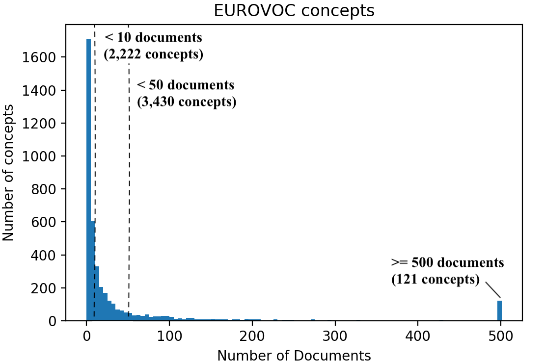
Figure 1: EUROVOC concepts frequency.

The labels of eurlex57k are divided in three categories: frequent labels (746), which occur in more than 50 training documents and can be found in all three subsets (training, development, test); few-shot labels (3,362), which appear in 1 to 50 training documents; and zero-shot labels (163), which appear in the development and/or test, but not in the training, documents.

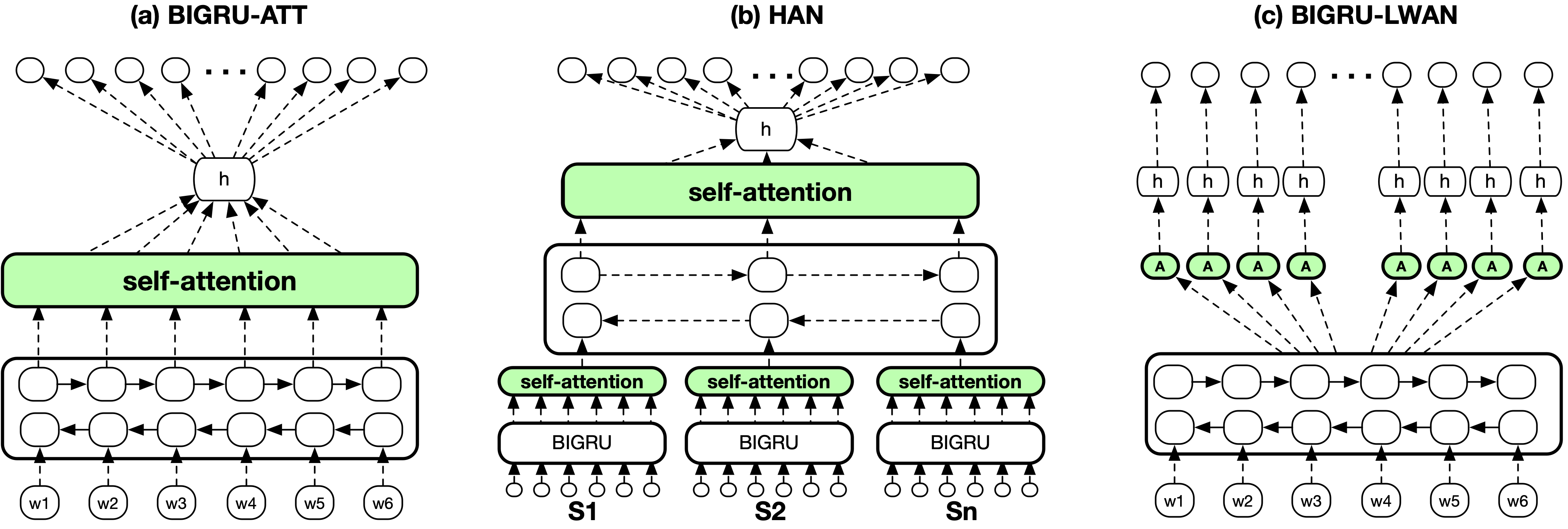
Figure 2: Illustration of (a) bigru-att, (b) han, and (c) bigru-lwan.

4 Methods Considered

We experiment with a wide repertoire of methods including linear and non-linear neural classifiers. We also propose and conduct initial experiments with two novel neural methods that aim to cope with the extended length of the legal documents and the information sparsity (for xmtc purposes) across the sections of the documents.

4.1 Baselines

4.1.1 Exact Match

To demonstrate that plain label name matching is not sufficient, our first weak baseline, Exact Match, tags documents only with labels whose descriptors appear verbatim in the documents.

4.1.2 Logistic Regression

To demonstrate the limitations of linear classifiers with bag-of-words representations, we train a Logistic Regression classifier with tf-idf scores for the most frequent unigrams, bigrams, trigrams, 4-grams, 5-grams across all documents. Logistic regression with similar features has been widely used for multi-label classification in the past.

4.2 Neural Approaches

We present eight alternative neural methods. In the following subsections, we describe their structure consisting of five main parts:

• word encoder (enc_w): turns word embeddings into context-aware embeddings,

• section encoder (enc_s): turns each section (sentence) into a sentence embedding,

• document encoder (enc_d): turns an entire document into a final dense representation,

• section decoder (dec_s) or document decoder (dec_d): maps the section or document representation to a many-hot label assignment.

All parts except for enc_w and dec_d are optional, i.e., they may not be present in all methods.

4.2.1 BIGRU-ATT

In the first deep learning method, bigru-att (Figure 2a), enc_w is a stack of bigrus that converts the pre-trained word embeddings ($w_{t}$) to context-aware ones ($h_{t}$). enc_d employs a self attention mechanism to produce the final representation $d$ of the document as a weighted sum of $h_{t}$:

$$a_{t} = \frac{\mathrm{exp}(h_{t}^{\top}u)}{\sum_{j}\mathrm{exp}(h_{j}^{\top}u)}$$ (1)

$$d = \frac{1}{T}\sum^{T}_{t=1}a_{t}h_{t}$$ (2)

$T$ is the document’s length in words, and $u$ is a trainable vector used to compute the attention scores $a_{t}$ over $h_{t}$. dec_d is a linear layer with $L=4,271$ output units and sigmoid ($\operatorname{\sigma}$) activations that maps the document representation $d$ to $L$ probabilities, one per label.

4.2.2 HAN

The Hierarchical Attention Network (han) Yang et al. (2016), exploits the structure of the documents by encoding the text in two consecutive steps (Figure 2b). First, a bigru (enc_w) followed by a self-attention mechanism (enc_s) turns the word embeddings ($w_{it}$) of each section $s_{i}$ with $T_{i}$ words into a section embedding $c_{i}$:

$$v_{it} = \tanh(W^{(s)}h_{it}+b^{(s)})$$ (3)

$$a^{(s)}_{it} = \frac{\mathrm{exp}(v_{it}^{\top}u^{(s)})}{\sum_{j}\mathrm{exp}(v_{ij}^{\top}u^{(s)})}$$ (4)

$$c_{i} = \frac{1}{T_{i}}\sum^{T_{i}}_{t=1}a^{(s)}_{it}h_{it}$$ (5)

where $u^{(s)}$ is a trainable vector. Next, enc_d, another bigru with self-attention, converts the section embeddings ($S$ in total, as many as the sections) to the final document representation $d$:

$$v_{i} = \tanh(W^{(d)}c_{i}+b^{(d)})$$ (6)

$$a^{(d)}_{i} = \frac{\mathrm{exp}(v_{i}^{\top}u^{(d)})}{\sum_{j}\mathrm{exp}(v_{j}^{\top}u^{(d)})}$$ (7)

$$d = \frac{1}{S}\sum^{S}_{i=1}a^{(d)}_{i}c_{i}$$ (8)

where $u^{(d)}$ is a trainable vector. The final decoder dec_d of han is the same as in bigru-att.

4.3 MAX-HSS

Initial experiments we conducted indicated that han is outperformed by the shallower bigru-att. We suspected that the main reason was the fact that the section embeddings $c_{i}$ that han’s enc_s produces contain useful information that is later degraded by han’s enc_d. Based on this assumption, we experimented with a novel method, named Max-Pooling over Hierarchical Attention Scorers (max-hss). max-hss produces section embeddings $c_{i}$ in the same way as han, but then employs a separate dec_s per section to produce label predictions from each section embedding $c_{i}$:

$$p^{(s)}_{i}=\operatorname{\sigma}(W^{(m)}c_{i}+b^{(m)})$$ (9)

where $p_{i}$ is an $L$-dimensional vector containing probabilities for all labels, derived from $c_{i}$. dec_d aggregates the predictions for the whole document with a maxpool operator that extracts the highest probability per label across all sections:

$$p^{(d)}=\textsc{maxpool}(p^{(s)}_{1},\dots,p^{(s)}_{S})$$ (10)

Intuitively, each section tries to predict the labels relying on its content independently, and dec_d extracts the most probable labels across sections.

4.3.1 CNN-LWAN and BIGRU-LWAN

The Label-wise Attention Network, lwan Mullenbach et al. (2018), also uses a self-attention mechanism, but here enc_d employs $L$ independent attention heads, one per label, generating $L$ document representations $d_{l}=\sum_{t}a_{lt}h_{t}$ ($l=1,\dots,L$) from the sequence of context aware word embeddings $h_{1},\dots,h_{T}$ of each document $d$. The intuition is that each attention head focuses on possibly different aspects of $h_{1},\dots,h_{T}$ needed to decide if the corresponding label should be assigned to the document or not. dec_d employs $L$ linear layers with $\operatorname{\sigma}$ activation, each one operating on a label-wise document representation $d_{l}$ to produce the probability for the corresponding label. In the original lwan (Mullenbach et al., 2018), called cnn-lwan here, enc_w is a vanilla cnn. We use a modified version, bigru-lwan, where enc_w is a bigru (Figure 2c).

4.4 Z-CNN-LWAN and Z-BIGRU-LWAN

Following the work of Mullenbach et al. (2018), Rios and Kavuluru (2018b) designed a similar architecture in order to improve the results in documents that are classified with rare labels. In one of their models, enc_d creates label representations, $u_{l}$, from the corresponding descriptors as follows:

$$u_{l}=\frac{1}{E}\sum^{E}_{e=1}w_{le}$$ (11)

where $w_{le}$ is the word embedding of the $e$-th word in the $l$-th label descriptor. The label representations are then used as alternative attention vectors:

$$v_{t} = \tanh(W^{(z)}h_{t}+b^{(z)})$$ (12)

$$a_{lt} = \frac{\mathrm{exp}(v_{t}^{\top}u_{l})}{\sum_{j}\mathrm{exp}(v_{j}^{\top}u_{l})}$$ (13)

$$d_{l} = \frac{1}{T}\sum^{T}_{t=1}a_{lt}h_{t}$$ (14)

where $h_{t}$ are the context-aware embeddings produced by a vanilla cnn (enc_w) operating on the document’s word embeddings, $a_{lt}$ are the attention scores conditioned on the corresponding label representation $u_{l}$, and $d_{l}$ is the label-wise document representation. dec_d also relies on label representations to produce each label’s probability:

$$p_{l} = \operatorname{\sigma}(u_{l}^{\top}d_{l})$$ (15)

Note that the representations $u_{l}$ of both encountered (during training) and unseen (zero-shot) labels remain unchanged, because the word embeddings $w_{le}$ are not updated (Eq. 11). This keeps the representations of zero-shot labels close to those of encountered labels they share several descriptor words with. In turn, this helps the attention mechanism (Eq. 13) and the decoder (Eq. 15), where the label representations $u_{l}$ are used, cope with unseen labels that have similar descriptors with encountered labels. As with cnn-lwan and bigru-lwan, we experiment with the original version of the model of Rios and Kavuluru (2018b), which uses a cnn enc_w (z-cnn-lwan), and a version that uses a bigru enc_w (z-bigru-lwan).

4.5 LW-HAN

We also propose a new method, Label-Wise Hierarchical Attention Network (lw-han), that combines ideas from both han and lwan. For each section, lw-han employs an lwan to produce $L$ probabilities. Then, like max-hss, a maxpool operator extracts the highest probability per label across all sections. In effect, lw-han exploits the document structure to cope with the extended document length of legal documents, while employing multiple label-wise attention heads to deal with the vast and sparse label set. By contrast, max-hss does not use label-wise attention.

5 Experimental Results

5.1 Experimental Setup

Hyper-parameters were tuned on development data using hyperopt. We tuned for the following hyper-parameters and ranges: enc output units {200, 300, 400}, enc layers {1, 2}, batch size {8, 12, 16}, dropout rate {0.1, 0.2, 0.3, 0.4}, word dropout rate {0.0, 0.01, 0.02}. For the best hyper-parameter values, we perform five runs and report mean scores on test data. For statistical significance, we take the run of each method with the best performance on development data, and perform two-tailed approximate randomization tests Dror et al. (2018) on test data. We used 200-dimensional pre-trained glove embeddings Pennington et al. (2014) in all neural methods.

5.2 Evaluation Measures

The most common evaluation measures in xmtc are recall ($R@K$), precision ($P@K$), and nDCG ($\textit{nDCG}@K$) at the top $K$ predicted labels, along with micro-averaged $F$-1 across all labels. Measures that macro-average over labels do not consider the number of instances per label, thus being very sensitive to infrequent labels, which are many more than frequent ones (Section 3.2). On the other hand, ranking measures, like $R@K$, $P@K$, $\textit{nDCG}@K$, are sensitive to the choice of $K$. In eurlex57k the average number of labels per document is 5.07, hence evaluating at $K=5$ is a reasonable choice. We note that 99.4% of the dataset’s documents have at most 10 gold labels.

While $R@K$ and $P@K$ are commonly used, we question their suitability for xmtc. $R@K$ leads to unfair penalization of methods when documents have more than $K$ gold labels. Evaluating at $K=1$ for a document with $N>1$ gold labels returns at most $R@1=\frac{1}{N}$, unfairly penalizing systems by not allowing them to return $N$ labels. This is shown in Figure 3, where the green lines show that $R@K$ decreases as $K$ decreases, because of low scores obtained for documents with more than $K$ labels. On the other hand, $P@K$ leads to excessive penalization for documents with fewer than $K$ gold labels. Evaluating at $K=5$ for a document with just one gold label returns at most $P@5=\frac{1}{5}=0.20$, unfairly penalizing systems that retrieved all the gold labels (in this case, just one). The red lines of Figure 3 decline as $K$ increases, because the number of documents with fewer than $K$ gold labels increases (recall that the average number of gold labels is 5.07).

Figure 3: $R@K$ (green lines), $P@K$ (red), $RP@K$ (black) scores of the best methods (bigru-att, hans, bigru-lwan), for $K=1$ to 10. All scores macro-averaged over test documents.

Similar concerns have led to the introduction of $\mathrm{R}\text{-}\mathrm{Precision}$ and $\textit{nDCG}@K$ in Information Retrieval Manning et al. (2009), which we believe are also more appropriate for xmtc. Note, however, that $\mathrm{R}\text{-}\mathrm{Precision}$ requires that the number of gold labels per document is known beforehand, which is not realistic in practical applications. Therefore we propose $\mathrm{R}\text{-}\mathrm{Precision}@K$ ($RP@K$) where $K$ is the maximum number of retrieved labels. Both $RP@K$ and $\textit{nDCG}@K$ adjust to the number of gold labels per document, without unfairly penalizing systems for documents with fewer than $K$ or many more than $K$ gold labels. They are defined as follows:

$$RP@K=\frac{1}{N}\sum^{N}_{n=1}\sum^{K}_{k=1}\frac{\mathrm{Rel}(n,k)}{\min{(K,R_{n})}}$$ (16)

$$\textit{nDCG}@K=\frac{1}{N}\sum^{N}_{n=1}Z_{Kn}\sum^{K}_{k=1}\frac{2^{\mathrm{Rel}(n,k)}-1}{\log_{2}{(1+k)}}$$ (17)

Here $N$ is the number of test documents; $\mathrm{Rel}(n,k)$ is 1 if the $k$-th retrieved label of the $n$-th test document is correct, otherwise 0; $R_{n}$ is the number of gold labels of the $n$-th test document; and $Z_{Kn}$ is a normalization factor to ensure that $\textit{nDCG}@K=1$ for perfect ranking.

In effect, $RP@K$ is a macro-averaged (over test documents) version of $P@K$, but $K$ is reduced to the number of gold labels $R_{n}$ of each test document, if $K$ exceeds $R_{n}$. Figure 3 shows $RP@K$ for the three best systems. Unlike $P@K$, $RP@K$ does not decline sharply as $K$ increases, because it replaces $K$ by $R_{n}$ (number of gold labels) when $K>R_{n}$. For $K=1$, $RP@K$ is equivalent to $P@K$, as confirmed by Fig. 3. For large values of $K$ that almost always exceed $R_{n}$, $RP@K$ asymptotically approaches $R@K$ (macro-averaged over documents), as also confirmed by Fig. 3.

	All Labels			Frequent		Few		Zero
	$RP@5$	$nDCG@5$	Micro-$F1$	$RP@5$	$nDCG@5$	$RP@5$	$nDCG@5$	$RP@5$	$nDCG@5$
Exact Match	0.097	0.099	0.120	0.219	0.201	0.111	0.074	0.194	0.186
Logistic Regression	0.710	0.741	0.539	0.767	0.781	0.508	0.470	0.011	0.011
bigru-att	0.758	0.789	0.689	0.799	0.813	0.631	0.580	0.040	0.027
han	0.746	0.778	0.680	0.789	0.805	0.597	0.544	0.051	0.034
cnn-lwan	0.716	0.746	0.642	0.761	0.772	0.613	0.557	0.036	0.023
bigru-lwan	0.766	0.796	0.698	0.805	0.819	0.662	0.618	0.029	0.019
z-cnn-lwan	0.684	0.717	0.618	0.730	0.745	0.495	0.454	0.321	0.264
z-bigru-lwan	0.718	0.752	0.652	0.764	0.780	0.561	0.510	0.438	0.345
ensemble-lwan	0.766	0.796	0.698	0.805	0.819	0.662	0.618	0.438	0.345
max-hss	0.737	0.773	0.671	0.784	0.803	0.463	0.443	0.039	0.028
lw-han	0.721	0.761	0.669	0.766	0.790	0.412	0.402	0.039	0.026

Table 2: Results on eurlex57k for all, frequent ($>50$ training instances), few-shot (1 to 50 instances), and zero-shot labels. All the differences between the best (bold) and other methods are statistically significant ($p<0.01$).

5.3 Overall Experimental Results

Table 2 reports experimental results for all methods and evaluation measures. As expected, Exact Match is vastly outperformed by machine learning methods, while Logistic Regression is also unable to cope with the complexity of xmtc.

In Section 2, we referred to the lack of previous experimental comparison between methods relying on label-wise attention and strong generic text classification baselines. Interestingly, for all, frequent, and even few-shot labels, the generic bigru-att performs better than cnn-lwan, which was designed for xmtc. han also performs better than cnn-lwan for all and frequent labels. However, replacing the cnn encoder of cnn-lwan with a bigru (bigru-lwan) leads to the best results overall, with the exception of zero-shot labels, indicating that the main weakness of cnn-lwan is its vanilla cnn encoder.

5.4 Few-shot and Zero-shot Results

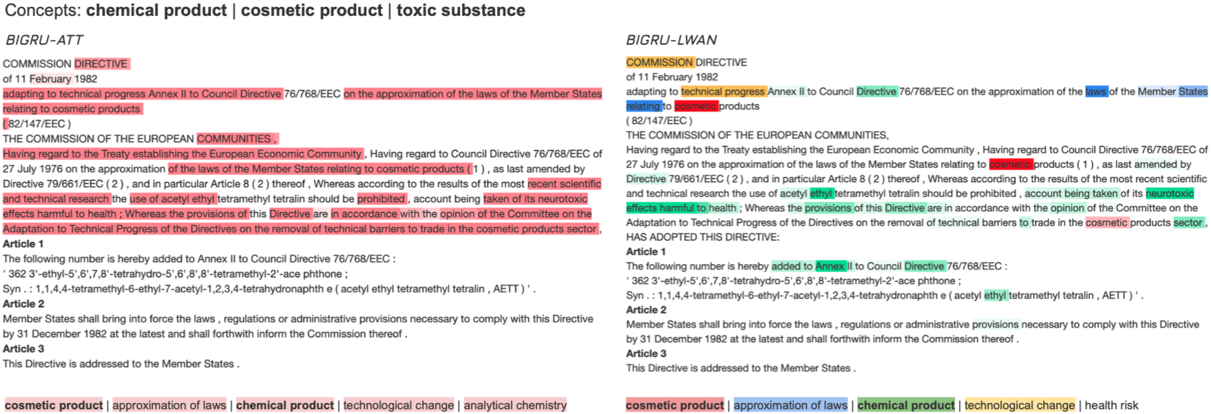
(a) COMMISSION DIRECTIVE (EEC) No 82/147

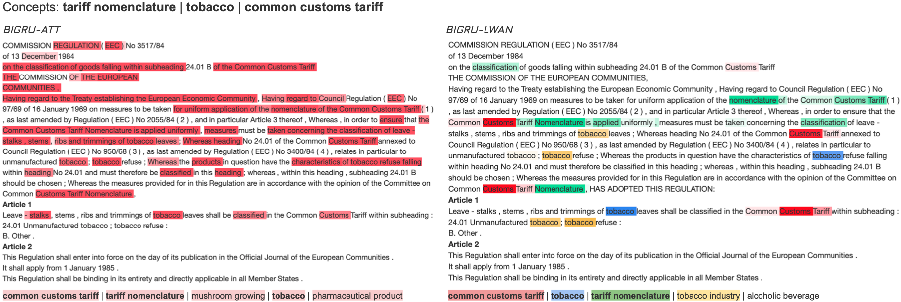
(b) COMMISSION REGULATION (EEC) No 3517/84

Figure 4: Attention heat-maps for bigru-att (left) and bigru-lwan (right). Gold labels (concepts) are shown at the top of each sub-figure, while the top 5 predicted labels are shown at the bottom. Correct predictions are shown in bold. bigru-lwan’s label-wise attentions are depicted in different colors.

As noted by Rios and Kavuluru Rios and Kavuluru (2018b), developing reliable and robust classifiers for few-shot and zero-shot tasks is a significant challenge. Consider, for example, a test document referring to concepts that have rarely (few-shot) or never (zero-shot) occurred in training documents (e.g., ‘tropical disease’, which exists once in the whole dataset). A reliable classifier should be able to at least make a good guess for such rare concepts.

As shown in Table 2, bigru-lwan outperforms all other methods in both frequent and few-shotlabels, but not in zero-shot labels, where z-cnn-lwan Rios and Kavuluru (2018b) provides exceptional results compared to other methods. Again, replacing the vanilla cnn of z-cnn-lwan with a bigru (z-bigru-lwan) improves performance across all label types and measures.

All other methods, including bigru-att, han, lwan, fail to predict relevant zero-shot labels (Table 2). This behavior is not surprising, because the training objective, minimizing binary cross-entropy across all labels, largely ignores infrequent labels. The zero-shot versions of cnn-lwan and bigru-lwan outperform all other methods on zero-shot labels, in line with the findings of Rios and Kavuluru (2018b), because they exploit label descriptors, which they do not update during training (Section 4.4). Exact Match also performs better than most other methods (excluding z-cnn-lwan and z-bigru-lwan) on zero-shot labels, because it exploits label descriptors.

To better support all types of labels (frequent, few-shot, zero-shot), we propose an ensemble of bigru-lwan and z-bigru-lwan, which outputs the predictions of bigru-lwan for frequent and few-shot labels, along with the predictions of z-bigru-lwan for zero-shot labels. The ensemble’s results for ‘all labels’ in Table 2 are the same as those of bigru-lwan, because zero-shot labels are very few (163) and rare in the test set.

The two methods (max-hss, lw-han) that aggregate (via maxpool) predictions across sections under-perform in all types of labels, suggesting that combining predictions from individual sections is not a promising direction for xmtc.

5.5 Providing Evidence through Attention

Chalkidis and Kampas (2018) noted that self-attention does not only lead to performance improvements in legal text classification, but might also provide useful evidence for the predictions (i.e., assisting in decision-making). On the left side of Figure 4(a), we demonstrate such indicative results by visualizing the attention heat-maps of bigru-att and bigru-lwan. Recall that bigru-lwan uses a separate attention head per label. This allows producing multi-color heat-maps (a different color per label) separately indicating which words the system attends most when predicting each label. By contrast, bigru-att uses a single attention head and, thus, the resulting heat-maps include only one color.

6 Conclusions and Future Work

We compared various neural methods on a new legal xmtc dataset, eurlex57k, also investigating few-shot and zero-shot learning. We showed that bigru-att is a strong baseline for this xmtc dataset, outperforming cnn-lwan Mullenbach et al. (2018), which was especially designed for xmtc, but that replacing the vanilla cnn of cnn-lwan by a bigru encoder (bigru-lwan) leads to the best overall results, except for zero-shot labels. For the latter, the zero-shot version of cnn-lwan of Rios and Kavuluru (2018b) produces exceptional results, compared to the other methods, and its performance improves further when its cnn is replaced by a bigru (z-bigru-lwan). Surprisingly han Yang et al. (2016) and other hierarchical methods we considered (max-hss, lw-han) are weaker compared to the other neural methods we experimented with, which do not consider the structure (sections) of the documents.

The best methods of this work rely on grus and thus are computationally expensive. The length of the documents further affects the training time of these methods. Hence, we plan to investigate the use of Transformers Vaswani et al. (2017); Dai et al. (2019) and dilated cnns Kalchbrenner et al. (2017) as alternative document encoders.

Given the recent advances in transfer learning for natural language processing, we plan to experiment with pre-trained neural language models for feature extraction and fine-tuning using state-of-the-art approaches such as elmo Peters et al. (2018)), ulmfit Howard and Ruder (2018) and bert Devlin et al. (2019).

Finally, we also plan to investigate further the extent to which attention heat-maps provide useful explanations of the predictions made by legal predictive models following recent work on attention explainability Jain and Wallace (2019).

References

- Aletras et al. (2016) Nikolaos Aletras et al. 2016. Predicting judicial decisions of the European Court of Human Rights: a Natural Language Processing perspective. PeerJ Computer Science, 2:e93.
- Bhatia et al. (2015) Kush Bhatia, Himanshu Jain, Purushottam Kar, Manik Varma, and Prateek Jain. 2015. Sparse Local Embeddings for Extreme Multi-label Classification. In Advances in Neural Information Processing Systems 28, pages 730–738.
- Bojanowski et al. (2016) Piotr Bojanowski, Edouard Grave, Armand Joulin, and Tomas Mikolov. 2016. Enriching Word Vectors with Subword Information. arXiv preprint arXiv:1607.04606.
- Chalkidis et al. (2017) Ilias Chalkidis, Ion Androutsopoulos, and Achilleas Michos. 2017. Extracting Contract Elements. In Proceedings of the 16th International Conference on Artificial Intelligence and Law, pages 19–28.