Cavity-photon induced high order transitions between ground states of quantum dots

Abstract

We show that quantum electromagnetic transitions to high orders are essential to describe the time-dependent path of a nanoscale electron system in a Coulomb blockage regime when coupled to external leads and placed in a three-dimensional rectangular photon cavity. The electronic system consists of two quantum dots embedded asymmetrically in a short quantum wire. The two lowest in energy spin degenerate electron states are mostly localized in each dot with only a tiny probability in the other dot. In the presence of the leads we identify a slow high order transition between the ground states of the two quantum dots. The Fourier power spectrum for photon-photon correlations in the steady state shows a Fano-type of a resonance for the frequency of the slow transition. Full account is taken of the geometry of the multi-level electronic system, and the electron-electron Coulomb interactions together with the para- and diamagnetic electron-photon interactions are treated with step wise exact numerical diagonalization and truncation of appropriate many-body Fock spaces. The matrix elements for all interactions are computed analytically or numerically exactly.

I Introduction

Many research groups are studying the physics of strong and ultrastrong coupling of light and matter in atomic or circuit-QED systems, or semiconductor heterostructures with the aid of photon cavities Petersson et al. (2012); Niemczyk et al. (2010); Ates et al. (2009); Yoshie et al. (2004); Reithmaier et al. (2004). Some aspects of this research has been addressed in review articles recently Cottet et al. (2017); Frisk Kockum et al. (2019). The research is carried out with multiple aim or goals in mind, ranging from optoelectronic or quantum computing devices to a convenient platform to study fundamental aspects of strong matter-light interactions.

In a recent article Zhang et al. Zhang et al. (2016) stress the importance of the possibilities of the two-dimensional electron system (2DES) in the conduction band of a GaAs heterostructure to obtain a collective nonperturbative coupling of 2D electrons with high-quality-factor terahertz cavity photons. They report experiments using cyclotron resonances between Landau levels to achieve both a small cavity-photon decay constant, and a low electron decoherence rate. Interestingly, they find that a model including the diamagnetic electron-photon interaction best fits their results. The electron system in the cavity is not coupled to external leads functioning as electron reservoirs. Theoretically Ciuti et al. (2005), and experimentally Dini et al. (2003), intersubband transitions in cavities have been studied earlier.

The addition of metallic electron reservoirs has been experimented with Cottet et al. (2017), which could lead the way to hybrid electron-photonic transport systems, that would still enhance the possible utility of the systems in devices and fundamental research.

In the last five years we have been developing an approach to model the time-dependent transport of electrons through a nanoscale electronic system embedded in a photon cavity. The main emphasis has been on multilevel systems with a specific shape or geometry, higher order interactions between electrons, and electrons and photons, and a time scale spanning the transient to the steady-state regime. To accomplish this we have used a generalized master equations and exact numerical diagonalization to study various effects Abdulla et al. (2019); Gudmundsson et al. (2018, 2018); Dinu et al. (2018).

At the formal level, we refine the calculation of both the para- and the diamagnetic contributions to the electron-photon interaction. The corresponding matrix elements are calculated exactly for a specific type of a cavity, a three-dimensional rectangular one. By doing so we are able to test the validity of the usual lowest order approximation with respect to the ratio of the size of the 3D cavity to the length of the central electronic system. This is an important step, especially in order to establish the correct form of the diamagnetic (i.e. A-square) term. Second, and more important, we want to stress that nonperturbative approach to the electron-photon interactions is not only necessary for the strong and the ultrastrong coupling regime, but also when electromagnetic transitions or tunneling through photon active states can take a very long time. This can be the case for transitions in a terahertz cavity containing a GaAs heterostructure with active intersubband processes.

Our central system has two well separated quantum dots so that we find the two states with the lowest energy (each one with their two spin components) almost entirely localized in either dot, with only a tiny overlap with the other. We will show that when the dot lower in energy is in a Rabi-resonance with the excited states within the bias window set by the external leads there is still a very slow high order photon active transition between the “ground states” of the dots.

The model and the improved electron-photon coupling are introduced in Section II, the transport formalism along with the discussion of the numerical results are presented in Section III. We conclude in Section IV and include for completeness some technical results in two Appendices.

II The closed central system

We use a potential to describe the short parabolic quantum wire with two asymmetrically embedded quantum dots Gudmundsson et al. (2019)

$$V(x,y)= \left[\frac{1}{2}m^{*}\Omega_{0}^{2}y^{2}-eV_{g}+\theta\left(\frac{L_{x}}{2}-|x|\right)\right.$$ (1)

$$\times \left.\sum_{i=1}^{2}V_{d}^{i}\exp{\left\{-\beta_{i}^{2}(x-x_{0i})^{2}-\beta_{i}^{2}(y-y_{0i})^{2}\right\}}\right]$$

with the parameters $\hbar\Omega_{0}=2.0$ meV, $V_{d}^{1}=-6.6$ meV, $V_{d}^{2}=-6.8$ meV, $\beta_{1}=0.030$ nm^-1, $\beta_{2}=0.028$ nm^-1, $x_{01}=-48$ nm, $x_{02}=+48$ nm, $y_{01}=-50$ nm, $y_{02}=+50$ nm, $L_{x}=180$ nm. $\theta$ is the Heaviside unit step function, and $V_{g}$ is the plunger gate voltage used to shift the energy of electronic states with respect to the bias window that will be defined by the chemical potentials of the left (L) and right (R) leads.

In terms of field operators for the electrons in the conduction band of GaAs the current density and the probability density operators are

$$\mathbf{j}=-\frac{e}{2m}\left\{\psi^{\dagger}\bm{\pi}\psi+\bm{\pi}^{*}\psi^{\dagger}\psi\right\},\quad\rho=\psi^{\dagger}\psi,$$ (2)

with

$${\bm{\pi}}=\left(\mathbf{p}+\frac{e}{c}\mathbf{A}_{\mathrm{ext}}\right),$$ (3)

where the external homogeneous magnetic field perpendicular to the plane of the central two-dimensional (2D) system is represented by the classical vector potential $\mathbf{A}_{\mathrm{ext}}=(-By,0,0)$. The external magnetic field $B=0.1$ T and the parabolic confinement energy $\hbar\Omega_{0}=2.0$ meV in the $y$-direction for the central system (and the semi-infinite external leads) define a convenient length scale $a_{w}=(\hbar/(m^{*}\Omega_{w}))^{1/2}$, where $\hbar\Omega_{w}=\hbar({\omega_{c}^{2}+\Omega_{0}^{2}})^{1/2}$, and $\omega_{c}=(eB_{\mathrm{ext}})/(m^{*}c)$. For the GaAs parameters used here, $m^{*}=0.067m_{e}$, $\kappa_{e}=12.4$, and $g^{*}=-0.44$, we have $a_{w}\approx 23.8$ nm. The main role of the external magnetic field is to lift spin and orbital degeneracies without introducing considerable orbital magnetic effects for the small system. The Hamiltonian for the central system is

$$H_{\mathrm{S}}= \int d^{2}r\psi^{\dagger}(\mathbf{r})\left\{\frac{\pi^{2}}{2m^{*}}+V(\mathbf{r})\right\}\psi(\mathbf{r})$$

$$+ H_{\mathrm{EM}}+H_{\mathrm{Coul}}+H_{\mathrm{Z}}$$

$$+ \frac{1}{c}\int d^{2}r\;\mathbf{j}(\mathbf{r})\cdot\mathbf{A}_{\gamma}+\frac{e^{2}}{2m^{*}c^{2}}\int d^{2}r\;\rho(\mathbf{r})A_{\gamma}^{2},$$ (4)

where $H_{\mathrm{EM}}=\hbar\omega a^{\dagger}a$ is the Hamiltonian for the single cavity mode with energy $\hbar\omega$, $H_{\mathrm{Z}}$ is the Zeeman term for the electrons, and $H_{\mathrm{Coul}}$ is the mutual Coulomb interaction of the electrons with kernel

$$V_{\mathrm{Coul}}(\mathbf{r}-\mathbf{r}^{\prime})=\frac{e^{2}}{\kappa_{e}\sqrt{|\mathbf{r}-\mathbf{r}^{\prime}|^{2}+\eta_{c}^{2}}},$$ (5)

and a small regularization parameter $\eta_{c}/a_{w}=3\times 10^{-7}$.

The first term in the third line of Eq. (II) is the paramagnetic electron-photon interaction, while the second term is the diamagnetic part of the interaction.

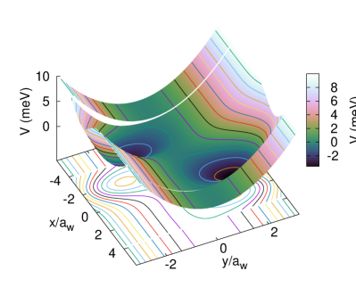
Figure 1: The potential defining the short parabolic quantum wire with two asymmetrically embedded quantum dots. The length of the short wire is $L_{x}=180$ nm. $a_{w}=23.8$ nm, and the short wire extends from $x/a_{w}\approx-3.8$ to $x/a_{w}\approx+3.8$, beyond which limits are indicated the semi-infinite leads (separated by narrow gaps in the figure) that are coupled to the short quantum wire at $t=0$.

We assume a rectangular photon-cavity of dimensions $a_{\mathrm{c}}\times b_{\mathrm{c}}\times d_{\mathrm{c}}$, and use a Coulomb gauge for the quantized vector potential $\mathbf{A}_{\gamma}$ of the single-mode photon field of the cavity. The polarization of the electric field of the cavity photons parallel to the transport in the $x$-direction (with the unit vector $\mathbf{e}_{x}$) can be realized in the TE₀₁₁ mode, or perpendicular to it (defined by the unit vector $\mathbf{e}_{y}$) by the TE₁₀₁ mode. The quantized vector potential for the two polarizations for the cavity field can be expressed (in a stacked notation) as Gudmundsson et al. (2019)

$$\mathbf{A}_{\gamma}(\mathbf{r})=\left(\genfrac{}{}{0.0pt}{}{\hat{\mathbf{e}}_{x}}{\hat{\mathbf{e}}_{y}}\right){\cal A}\left\{a+a^{\dagger}\right\}\left(\genfrac{}{}{0.0pt}{}{\cos{\left(\frac{\pi y}{b_{\mathrm{c}}}\right)}}{\cos{\left(\frac{\pi x}{a_{\mathrm{c}}}\right)}}\right)\cos{\left(\frac{\pi z}{d_{\mathrm{c}}}\right)},$$ (6)

where the strength of the vector potential, ${\cal A}$, and the electron-photon coupling constant are related by $g_{\mathrm{EM}}=e{\cal A}\Omega_{w}a_{w}/c$. With the vector potential (6) and the fermionic field operators for the electrons the Hamiltonian for the electron-photon interactions becomes

$$H_{\mathrm{e-EM}}= g_{\mathrm{EM}}\sum_{ij}d^{\dagger}_{i}d_{j}g^{p}_{ij}\{a+a^{\dagger}\}$$ (7)

$$+ \frac{g_{\mathrm{EM}}^{2}}{\hbar\Omega_{w}}\sum_{ij}d^{\dagger}_{i}d_{j}g^{d}_{ij}\left[\left(a^{\dagger}a+\frac{1}{2}\right)+\frac{1}{2}(a^{\dagger}a^{\dagger}+aa)\right].$$

When the approximation that the wavelength of the cavity field is much larger than the size of the electronic system the second term of Eq. (7) becomes diagonal in the electronic creation and annihilation operators, i.e. $g^{d}_{ij}\rightarrow\delta_{i,j}$ Jonasson et al. (2012a, b); Gudmundsson et al. (2012). (It is important to note that the total diamagnetic interaction term is not diagonal, and thus we have found that it can lead to a very weak Rabi-splitting when the paramagnetic term is blocked by symmetry Gudmundsson et al. ) We will not make this approximation here, but use the fact that the original functional basis used to construct the single-electron basis for the short parabolic quantum wire Jonasson et al. (2012b) can be used to obtain the exact matrix elements for the electron-photon interaction analytically in a closed form. Technical details for the matrix elements, the energy spectra, and the many-body states are found in Appendix A.

In order to understand better the structure or properties of the states $|\breve{\mu})$ for one value of the coupling constant ($g_{\mathrm{EM}}=0.05$ meV) we show in Fig. 2 the energy of the lowest 64 states, together with their electron content, their spin $z$-component, and their mean photon number.

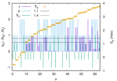
Figure 2: The energy (squares, right axis), the mean electron number (e), the mean photon number ($\gamma$), and the $z$-component of the spin, $S_{z}/\hbar$, as functions of the number of the many-body state, $\mu$. The horizontal black lines indicate the chemical potentials of the left, $\mu_{L}=1.4$ meV, and right leads, $\mu_{R}=1.1$ meV. $g_{\mathrm{EM}}=0.05$ meV, $B=0.1$ T, $L_{x}=180$ nm, $-eV_{g}=0.2$ meV, and $\hbar\omega=1.75$ meV.

We note that the lowest 4 states are one-electron states of which the lower ones with opposite spin $z$-component are mostly confined to the right quantum dot, while the higher ones are mostly confined to the left dot Gudmundsson et al. (2019). The fifth state is the vacuum or the empty state, while the sixth state is the spin-singlet two-electron ground state and $|\breve{7})$, $|\breve{8})$, and $|\breve{9})$ are the lowest in energy spin-triplet two-electron states. The next four states, $|\breve{10})$, $|\breve{11})$, $|\breve{12})$, and $|\breve{13})$ are the first replica of the one-electron ground state and the first excitation there of very close to a Rabi resonance, as can be verified by their mean photon content that is close to 1/2. These four states are in the bias window defined by the chemical potentials of the left and right leads. The next two states, $|\breve{14})$ $|\breve{15})$, are the first photon replicas of the one-electron states $|\breve{3})$ $|\breve{4})$ mostly localized in the left dot. The first excitations of $|\breve{3})$ $|\breve{4})$ are the next two states $|\breve{16})$ $|\breve{17})$ and we notice that the photon content of these four last states is close to an integer indicating that they are not close to a Rabi-resonance, but they are very weakly coupled by a Rabi resonance.

The position of the bias window gives a hint that the system most likely will approach a Coulomb blockage in the long time limit after the central system will be coupled to the external leads. Exactly, how this happens and the very different role of the four one-electron states below the bias window in the time evolution of the coupled system will be the subject of the study presented below.

For the cavity with photon energy $\hbar\omega=1.75$ meV the ratio of the size of the cavity to the length of the central system, $a_{c}/L_{x}$ or $b_{c}/L_{x}$, is 48.4 suggesting that corrections to the matrix elements of the electron-photon interaction due to the variation of the fields within the system size are minimal. This can indeed be verified by inspecting the change in self-energies of the lowest 32 many-body states presented in Fig. 3.

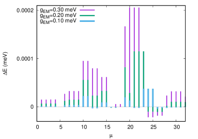
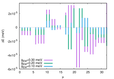
Figure 3: The change in self-energy caused by the exact form of the paramagnetic and diamagnetic electron-photon interactions of each many-body state $|\breve{\mu})$ for $x$- (upper) and $y$-polarized (lower) cavity field for three values of the coupling coefficient $g_{\mathrm{EM}}$. $B=0.1$ T, $L_{x}=180$ nm, $\hbar\Omega_{0}=2.0$ meV, $-eV_{g}=0.2$ meV, and $\hbar\omega=1.75$ meV.

This last statement should though be enjoyed with care. When the fields are assumed constant within the central electronic system the diamagnetic electron-photon interaction is diagonal and mainly contributes to the self-energy of the states, now with the exact matrix elements the contribution of the paramagnetic interaction to the self-energies is increased considerably, and the diamagnetic interaction is not anymore diagonal. These small changes in the form of the interactions can be of importance when investigating the very long time evolution of the system towards a steady state. An other important point is that the rather artificial diagonal form of the diamagnetic interaction is replaced. Results with the exact diamagnetic interaction can thus be used to verify how appropriate that form is. Below, we will use results from the time evolution of the system to learn to appreciate how important higher order electromagnetic transitions are to understand its properties and how far we are forced away from a perturbational view of the underlying processes.

Not surprisingly, we observe in Fig. 3 that the change in self-energy of the many-body states of the central system is larger for the $x$-polarized photon field. This reflects the anisotropy of the system, which is more easily polarized in the $x$-direction, that will be the direction of transport through it. Furthermore, we note that the change in the self-energy is nonlinear with $g_{\mathrm{EM}}$, even though $g_{\mathrm{EM}}$ is not large compared to the confinement energy $\hbar\Omega_{0}$.

III The electron transport, model and results

The central system is opened up for electron transport through it by coupling the left and right semi-infinite quasi-one-dimensional leads to it at $t=0$. The leads are assumed to have the same parabolic confinement in the $y$-direction as the central system and are subject to the same external homogeneous magnetic field. The coupling to the leads is described by the Hamiltonian

$$H_{T}=\theta(t)\sum_{il}\int d\mathbf{q}\left(T_{\mathbf{q}i}^{l}c_{\mathbf{q}l}^{\dagger}d_{i}+(T_{\mathbf{q}i}^{l})^{*}d_{i}^{\dagger}c_{\mathbf{q}l}\right),$$ (8)

where electrons in the short wire are created and annihilated by the operators $d_{i}^{\dagger}$ and $d_{i}$, respectively, but in the leads by the operators $c_{\mathbf{q}l}^{\dagger}$ and $c_{\mathbf{q}l}$. The quantum number $\mathbf{q}$ represents both the continuous momenta in the leads and a subband index. The coupling tensor $T_{\mathbf{q}i}^{l}$ is calculated using the probability density of each single-electron state of the lead $l$ and the central electron system in the contact region that is defined to extend approximately one $a_{w}$ into each subsystem Gudmundsson et al. (2009); Moldoveanu et al. (2009); Gudmundsson et al. (2012). At the same time, $t=0$, a photon reservoir of zero temperature is weakly coupled to the cavity with coupling coefficient $\kappa$. As the temperature of the photon reservoir is zero we can regard $\kappa$ as a cavity decay constant. The technical details for the method used to derive the master equation used to describe the transport calculations are found in Appendix B.

The structure of the master equation (11) associates a zero eigenvalue with the steady state of the system Petrosky (2010); Nakano et al. (2010). We thus display in Fig. 4 the logarithm of the absolute value of the eigenspectrum of $\mathfrak{L}$ as a function of the coupling parameter $g_{\mathrm{EM}}$.

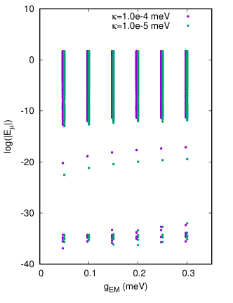
Figure 4: The logarithm of the absolute values of the complex eigenspectrum of the Liouville operator $\mathfrak{L}$ as a function of the electron-photon coupling coefficient $g_{\mathrm{EM}}$ for two values of the cavity-environment coupling $\kappa$. $B=0.1$ T, $-eV_{g}=0.2$ meV, and $L_{x}=180$ nm.

If we fix the gate voltage such that both spin components of the one-electron ground state are inside the bias window the system will not enter a Coulomb blockage regime, but conduct at a constant average rate in the steady state. In this case we always find a single zero eigenvalue. Here, when the system enters a Coulomb blockage regime we find a small null space of $\mathfrak{L}$ well separated by a spectral gap. Within the spectral gap we find one eigenvalue representing a very slow final transition in the system, that we will identify below. No transition in the null-space can be ignored as that would lead to a violation of the condition that $\mathrm{Tr_{\mathrm{S}}\{\rho_{\mathrm{S}}}\}=1$. The eigenvalues within the null-space are all zero within the machine and software accuracy that can be expected, even though they show some spread on the logarithmic scale adopted in Fig. 4.

The total mean number of electrons and photons is shown in Fig. 5 for three values of the cavity-environment coupling constant $\kappa$.

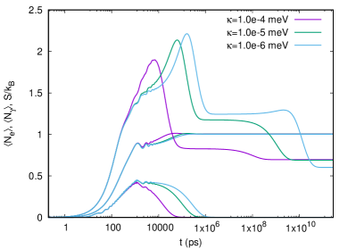
Figure 5: The entropy $S/k_{B}$, the mean electron, and the mean photon number as functions of time for the open central system for three different values of the cavity-environment coupling constant $\kappa$. For identification note, that in the steady-state the mean photon number seems to vanish, and the mean electron approaches 1. $g_{\mathrm{EM}}=0.1$ meV, $B=0.1$ T, $-eV_{g}=0.2$ meV, and $L_{x}=180$ nm.

The mean electron number can be identified as represented by the curves approaching 1 in the steady-state limit, but the curves representing the mean photon number seem to vanish in the same limit on the scale adopted for the figure. In addition, we show the Réniy-2 entropy of the central system Santos et al. (2017); Batalhao et al. (2018); Baez (2011)

$$S=-k_{B}\ln{[Tr(\rho^{2}_{\mathrm{S}})]}.$$ (9)

Interestingly, the entropy changes after the mean values of the total electron and photon numbers seem to have reached their steady-state values. A closer inspection finds that there is a tiny change in the mean photon number occurring in the same region as the last change in the entropy.

For completeness, we display in Fig. 6 the same information as in Fig. 5, but here we vary the coupling coefficient $g_{\mathrm{EM}}$ and keep $\kappa=1\times 10^{-5}$ meV.

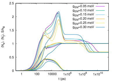
Figure 6: The entropy $S/k_{B}$, the mean electron, and the mean photon number as functions of time for the open central system for six different values of the electron-photon coupling constant $g_{\mathrm{EM}}$. For identification note, that in the steady-state the mean photon number seems to vanish, and the mean electron approaches 1. $\kappa=1\times 10^{-5}$ meV, $B=0.1$ T, $-eV_{g}=0.2$ meV, and $L_{x}=180$ nm.

The conclusion from both Fig. 5 and 6 is that judged from the entropy the on-set of the steady-state depends on both coupling parameters, $g_{\mathrm{EM}}$ and $\kappa$. This is not unexpected as they represent properties of the central system. The small oscillations visible in Fig. 5 and 6 in the range 400 – 10000 ps has been identified as coexisting nonequilibrium spin and Rabi oscillations Gudmundsson et al. (2019).

For the record, we mention that in a system of two parallel quantum dots and initially with only one photon found that after the mean electron and the mean current through the system seemed to have reached a steady-state value an internal photon active transition changing the state of the system Gudmundsson et al. (2017). In that case the system was not approaching the Coulomb blockage regime as the one-electron ground state was in the bias window, but initially there was no electron in the system, but one photon.

The last slow transition bringing the system to the steady-state in the Coulomb blockage regime can be identified by observing the time-dependent occupation of the many-body states in Fig. 7.

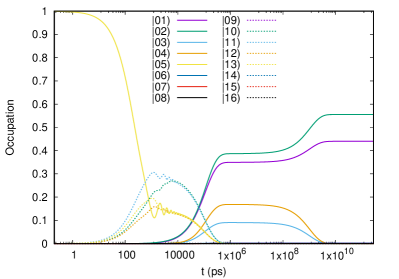
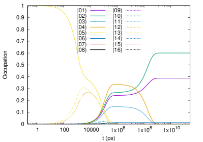
Figure 7: The occupation of selected many-body states $|\breve{\mu})$ as a function of time for $g_{\mathrm{EM}}=0.1$ meV (upper panel), and $g_{\mathrm{EM}}=0.3$ meV (lower panel). $\kappa=1\times 10^{-5}$ meV, $B=0.1$ T, $-eV_{g}=0.2$ meV, and $L_{x}=180$ nm. (The breve symbol is omitted here over the states).

In the upper panel of Fig. 7 for $g_{\mathrm{EM}}=0.1$ meV we observe the empty state $|\breve{5})$ “loosing occupation” as the states in the bias window, $|\breve{10})$, $|\breve{11})$, $|\breve{12})$, and $|\breve{13})$, gain occupation. These states in the bias window are Rabi-split with mean photon content close to $1/2$ and feed the two spin components of the one-electron ground state, $|\breve{1})$, and $|\breve{2})$, mostly localized in the right quantum dot, but also to a lesser extent the one-electron states, $|\breve{3})$, and $|\breve{4})$, mostly localized in the left quantum dot. The last transitions are thus from $|\breve{4})$ to $|\breve{2})$, and from $|\breve{3})$ to $|\breve{1})$. For the higher electron-photon coupling $g_{\mathrm{EM}}=0.3$ meV, shown in the lower panel of Fig. 7, similar processes take place with the exception that now an electron only enters into $|\breve{12})$, and $|\breve{13})$ as the states $|\breve{10})$ and $|\breve{11})$ are below the bias window. For this higher electron-photon coupling it comes more likely than before for the electron to enter states $|\breve{3})$, and $|\breve{4})$, and the transition to $|\breve{1})$, and $|\breve{2})$ goes faster. The lowering of states $|\breve{10})$ and $|\breve{11})$ below the bias window is the cause for the slower electron charging of the system in Fig. 6 for the last curve at $g_{\mathrm{EM}}=0.30$ meV.

A schema of the main transitions relevant for the approach to the steady-state is shown in Fig. 8.

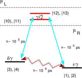
Figure 8: Schema of the main transitions leading to the steady-state. The azure arrows indicate the “low order” fast transitions connecting the Rabi-split states in the bias window to the lowest states in the quantum dots, but the wavy brown arrows indicate the high order slow transition connecting the lowest states mostly localized in either the left or the right quantum dot. The approximate lifetime of the transitions ($\tau$) is indicated. (The breve symbol is omitted here over the states).

We now turn our attention to these slow transitions. For $g_{\mathrm{EM}}=0.05$ meV the mean photon number for $|\breve{1})$, and $|\breve{2})$ is approximately $3.33\times 10^{-4}$ (indicated by $\epsilon\gamma$ in Fig. 8), and for $|\breve{3})$, and $|\breve{4})$ the mean number is $3.68\times 10^{-4}$ (indicated by $\delta\gamma$ in Fig. 8). Evaluated with a first order perturbation theory their mean photon number would vanish ($\epsilon=0$, $\delta=0$ in Fig. 8), and no first order photon active transition would exist between them unless the cavity frequency is set at resonance $\omega=0.3413$ meV, see Eq. (7). The transitions to the 4 lowest one-electron states from the photon replica states in the bias window do on the other hand exist in first order perturbation calculation. Then the dynamics corresponding to the azure lines could be described by an effective three-level $\Lambda$ model Scully and Zubairy (1997) for each spin orientation. As these resonant transitions become inactive around $t\sim 1$ $\mu$s, the $\Lambda$-picture fails and the system enters an apparent steady-state in the time range $t\in[1,100]$ $\mu$s. For the slow transitions, $|\breve{4})\rightarrow|\breve{2})$ and $|\breve{3})\rightarrow|\breve{1})$, the exact paramagnetic matrix elements are approximately 5 orders of magnitude larger than the diamagnetic ones. The sensitivity of the lifetime of the upper states, $|\breve{3})$ and $|\breve{4})$, on the electron-photon coupling makes us conclude that only some photon active higher order transitions are possible with a stronger para- than diamagnetic character. Supporting this claim is the behavior of the lifetime when the cavity-environment coupling $\kappa$ is varied (see Fig. 5). The shortened lifetime with increasing $\kappa$ reflects the Purcell effect on photon active transitions Purcell (1946), which was recently predicted to be visible in the transport current as a function of the photon energy in the steady-state Abdulla et al. (2019). The influence of $\kappa$ on the slow transition is clearly seen in the eigenspectrum of the Liouvillian in Fig. 4.

In the steady-state the Fourier spectral density of the emitted cavity radiation Gudmundsson et al.

$$S(E)=\frac{\kappa}{\pi}\left|\int_{0}^{\infty}\frac{d\tau}{\hbar}e^{-iE\tau/\hbar}\{\langle X(\tau)X(0)\rangle\}\right|,$$ (10)

with $X=a+a^{\dagger}$, is displayed in Fig. 9.

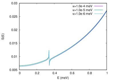
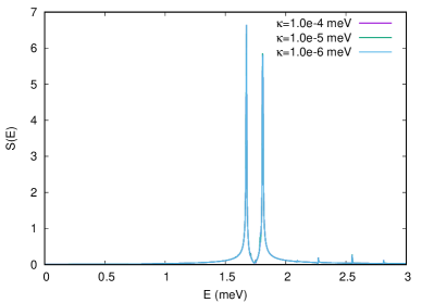
Figure 9: The Fourier power spectra for the photon correlation function $S(E)$ in the steady state for three values of the cavity-environment coupling $\kappa$. $g_{\mathrm{EM}}=0.1$ meV, $B=0.1$ T, $-eV_{g}=0.2$ meV, and $L_{x}=180$ nm.

On the coarser scale used in the lower panel of Fig. 9 are seen the two peaks split by approximately 0.135 meV, but centered around the energy of the cavity mode $\hbar\omega=1.75$ meV. The splitting corresponds to the Rabi splitting read from the energy spectrum. The finer scale used in the upper panel reveals a Fano-like resonance peak at the energy 0.3413 meV corresponding to the energy of the last slow transitions $|\breve{4})\rightarrow|\breve{2})$ and $|\breve{3})\rightarrow|\breve{1})$. The interpretation is that a very weak electromagnetic perturbation of the system in the steady-state (consisting mainly of the one-electron ground state) activates the transitions to the states in the bias window and the very slow transition from the spin components of the one-electron ground state to the states $|\breve{3})$ and $|\breve{4})$. Both types of excitations are radiative, or photon active, but are of a very different strength.

Last, a note on a curious emergence of a spin-polarization that can be seen in the steady-state in Fig. 7, where the polarization is increased in the lower panel, i.e. for a larger electron-photon coupling $g_{\mathrm{EM}}$. In Fig. 10 is plotted the mean value of the $z$-component of the spin as a function of time for three values of the cavity-environment coupling $\kappa$.

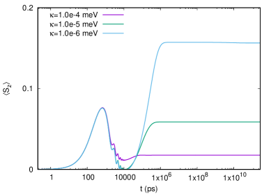
Figure 10: The mean $z$-component of the total spin, $S_{z}/\hbar$, as function of time for three different values of the cavity-environment coupling $\kappa$. $g_{\mathrm{EM}}=0.1$ meV, $B=0.1$ T, $-eV_{g}=0.2$ meV, and $L_{x}=180$ nm.

Clearly, the spin polarization in Fig. 7 is not caused by thermal effects, instead it is important to have in mind that the external semi-infinite leads are defined by a potential and have thus a quasi-one-dimensional electron system with subband structure. In addition, the system is in a weak external magnetic field $B=0.1$ T, and the probability of tunneling into the states in the bias window depends on the density of states of the leads and the shape of the states in the central electronic system. The small increase of the spin-polarization (note the small vertical scale of Fig. 10) is thus influenced by many factors as the path to the steady-state differs for different values of $\kappa$. This behavior can be related to the nonequilibrium spin-oscillations discussed earlier Gudmundsson et al. (2019).

IV Summary

In this report we have shown that in order to describe the time-evolution of electron transport through a nanoscale system in a GaAs heterostructure embedded in a terahertz cavity it is necessary to treat the electron-photon interaction nonperturbatively to make sure none of the vital transition is missed that takes the system finally to its steady state. On the long timescale needed some transitions forbidden in low order perturbation can be essential. Though the transition we take as an example has different symmetry, the difference in timescales possible are well know from, for example, the 2S$\rightarrow$1S in atomic hydrogen Fite et al. (1959); Choi et al. (1987); Parthey et al. (2011).

As expected in the terahertz range, the exact matrix elements for a rectangular photon-cavity do not change our results much, compared to matrix elements that are calculated assuming the field to be constant over the sample size of the nanoscale system. This is true as we anyway in both cases use a numerically exact diagonalization scheme to calculate the cavity-photon dressed many-body electron states and their energies. The higher order contributions are more important than the much smaller corrections caused by the shape of the cavity. But, it is important to remember that the exact matrix elements for the diamagnetic are not only diagonal in the electronic variables, and thus it is possible to find a transition caused by this term, that would otherwise go unnoticed, and might be comparable to the 2S$\rightarrow$1S transition in atomic hydrogen. Even, in the approximation that the electronic part of the interaction is diagonal the total interaction is not and can thus cause a tiny Rabi-splitting if that can be seen if the paramagnetic interaction is blocked by symmetry Gudmundsson et al. .

We interprete the results from our continuous model as showing a high order photon-cactive transtion between the ground states of weakly coupled quantum dots. In addition, we reconfirm the effects of the Purcell effect in a transport current Abdulla et al. (2019), and discover a slight spin polarization dependent on the cavity-decay or cavity-environment coupling constant $\kappa$ connected to non-equilibrium oscillations of the spin reported elsewhere Gudmundsson et al. (2019). We emphasize that even when we talk about photon active transitions it is important to remmeber that the coupling to the leads is a neccesary trigger in order to perturb the exact fully interacting eigenstates of the central system.

We hope to convey the message to the reader that details in the many-body description of the electron-photon interaction together with the geometry or shape of the systems can be of importance to understand promising electron-photonic systems, and through them we can hope to obtain better fundamental understanding of these interactions.

Appendix A Closed system: Technical details

The integrals for the matrix elements of the electron-photon interactions have integrands of three trigonometric functions over a finite interval or two Hermite polynomials, a Gaussian exponent and a trigonometric function over the infinite $y$-axis. After the matrix elements are found they are first transformed unitairily to the basis of 2688 exact single-electron functions for the short quantum wire in a perpendicular homogeneous magnetic field. Subsequently, after the construction of the 683 dimensional Fock many-body space using the 36 lowest in energy single-electron states, and the diagonalization of the Coulomb interaction therein the electron-photon matrix elements are transformed unitairily to the 512 dimensional truncated Fock space of exactly Coulomb interacting electrons. This last Fock space includes states with one, two and three electrons in a ratio adequate to its energy extension. The exact Coulomb interacting Fock space is then tensor multiplied by the 17 lowest eigenstates of the photon operator to form the Fock space used to diagonalize the electron-photon interaction in resulting in a 8704 dimensional many-body space of cavity-photon dressed electrons, of which we will use the 128 lowest in energy states to perform the transport calculations in. This step wise construction of the relevant many-body spaces and their truncation is necessary as a single-step construction would have required a much too large basis to attain an acceptable convergence, and an important fact to keep in mind is that the construction is much more sensitive to the number of electron states kept in the calculation than photon states, whose number is simple to increase. The reason for this is the polarization of charge by the electron-photon interaction. A rotating wave approximation is not used for the electron-photon interaction as in a complex central system with many states there might always be some transitions close to a Rabi resonance and other far from it.

The energy spectra as functions of the electron-photon coupling parameter $g_{\mathrm{EM}}$ for the many-body states of the fully interacting system are displayed in Fig. 11 for $x$-polarization of the cavity-photon field in the upper panels and $y$-polarization in the lower panels.

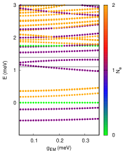
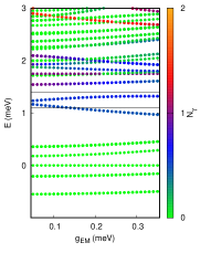
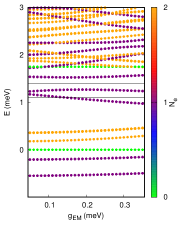
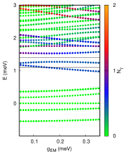
Figure 11: The many-body energy spectra as functions of the electron-photon coupling strength $g_{\gamma}$ for $x$-polarized (upper panels), and $y$-polarized (lower panels) cavity field. The mean electron number is color coded in the spectra (left panels), and the mean photon number (right panels). For a closed system the electron number is an integer, but not the photon number. $B=0.1$ T, $L_{x}=180$ nm, $\hbar\Omega_{0}=2.0$ meV, $-eV_{g}=0.2$ meV, and $\hbar\omega=1.75$ meV.

The many-body states $|\breve{\mu})$ are cavity-photon dressed electron states with an integer number of electrons indicated in the left panels, but their average photon content is shown in the right panels.

Appendix B Transport: Technical details

The time evolution the couplings to the reservoirs induce are best described by the Liouville-von Neumann equation for the probability operator (the density operator) of the total system, but as the continuous character of the respective reservoirs make the resulting Fock-space much too large we resort to the projection formalism of Nakajima Nakajima (1958) and Zwanzig Zwanzig (1960). Initially, we derive a non-Markovian generalized master equation (GME) for the reduced density operator of the central system including terms up to second order in the lead-system coupling (8) in the kernel of the resulting integro-differential equation Gudmundsson et al. (2012). Subsequently, we apply vectorization Petersen and Pedersen (2012) and Kronecker tensor products together with a Markovian approximation to transform the GME from the Fock-space of many-body states to the Liouville space of transitions Jonsson et al. (2017); Weidlich (1971). We include 128 Fock-states in our transport calculations and end thus up with 16384 transitions in the Liouville-space. The increased space size is counteracted by efficient parallelization and GPU-processing Jonsson et al. (2017). The weak photon dissipation is derived with a Markovian and rotating wave approximation, where the creation(annihilation) operator for the cavity-photons needs to be rid of fast rotating annihilation(creation) terms when transformed to the fully interacting basis $|\breve{\mu})$ in order for vacuum processes to be correctly described in the model Beaudoin et al. (2011); Gardiner and Collett (1985); Lax (1963); Gudmundsson et al. (2019).

Due to the vectorization Petersen and Pedersen (2012) the Markovian master equation in Liouville-space assumes the form of a simple linear first order differential equation Jonsson et al. (2017); Hohenester (2010)

$$\partial_{t}\operatorname{vec}(\rho_{\mathrm{S}})=-i\mathfrak{L}\operatorname{vec}(\rho_{\mathrm{S}}),$$ (11)

which has an analytical solution that is convenient to use to search for the steady-state of the system.

$$\operatorname{vec}(\rho_{\mathrm{S}}(t))=\left\{\mathfrak{U}\left[\exp{\left(-i\mathfrak{L}_{\text{diag}}t\right)}\right]\mathfrak{V}\right\}\operatorname{vec}(\rho_{\mathrm{S}}(0)),$$ (12)

with the left and right eigenvector matrices of the nonhermitian Liouville operator satisfying $\mathfrak{UV}=I$ and $\mathfrak{VU}=I$ Jonsson et al. (2017). The imaginary part of the eigenspectrum of the Liouville operator $\mathfrak{L}$ reveals the 16384 relaxation coefficients at work in the Markovian time evolution of the system.

References

- Petersson et al. (2012) K. D. Petersson, L. W. McFaul, M. D. Schroer, M. Jung, J. M. Taylor, A. A. Houck, and J. R. Petta, Nature 490, 380 (2012).
- Niemczyk et al. (2010) T. Niemczyk, F. Deppe, H. Huebl, E. P. Menzel, F. Hocke, M. J. Schwarz, J. J. Garcia-Ripoll, D. Zueco, T. Hümmer, E. Solano, A. Marx, and R. Gross, Nature Physics 6, 772 (2010).
- Ates et al. (2009) S. Ates, S. M. Ulrich, A. Ulhaq, S. Reitzestein, A. Löffler, S. Höfling, A. Forchel, and P. Michler, Nature Photonics 3, 724 (2009).
- Yoshie et al. (2004) T. Yoshie, A. Scherer, J. Hendrickson, G. Khitrova, H. M. Gibbs, G. Rupper, C. Ell, O. B. Shchekin, and D. G. Deppe, Nature 432, 200 (2004).
- Reithmaier et al. (2004) J. P. Reithmaier, G. Sek, A. Löffler, C. Hofmann, S. Kuhn, S. Reitzenstein, L. V. Keldysh, V. D. Kulakovskii, T. L. Reinecke, and A. Forchel, Nature 432, 197 (2004).
- Cottet et al. (2017) A. Cottet, M. C. Dartiailh, M. M. Desjardins, T. Cubaynes, L. C. Contamin, M. Delbecq, J. J. Viennot, L. E. Bruhat, B. Douçot, and T. Kontos, Journal of Physics: Condensed Matter 29, 433002 (2017).
- Frisk Kockum et al. (2019) A. Frisk Kockum, A. Miranowicz, S. De Liberato, S. Savasta, and F. Nori, Nature Reviews Physics 1, 19 (2019).
- Zhang et al. (2016) Q. Zhang, M. Lou, X. Li, J. L. Reno, W. Pan, J. D. Watson, M. J. Manfra, and J. Kono, Nature Physics 12, 1005 (2016).
- Ciuti et al. (2005) C. Ciuti, G. Bastard, and I. Carusotto, Phys. Rev. B 72, 115303 (2005).
- Dini et al. (2003) D. Dini, R. Köhler, A. Tredicucci, G. Biasiol, and L. Sorba, Phys. Rev. Lett. 90, 116401 (2003).
- Abdulla et al. (2019) N. R. Abdulla, C.-S. Tang, A. Manolescu, and V. Gudmundsson, arXiv:1905.07492 (2019).
- Gudmundsson et al. (2018) V. Gudmundsson, N. R. Abdullah, A. Sitek, H.-S. Goan, C.-S. Tang, and A. Manolescu, Physics Letters A 382, 1672 (2018).
- Gudmundsson et al. (2018) V. Gudmundsson, N. R. Abdullah, A. Sitek, H.-S. Goan, C.-S. Tang, and A. Manolescu, Annalen der Physik, 10.1002/andp.201700334 (2018), arXiv:1706.03483 [cond-mat.mes-hall] .
- Dinu et al. (2018) I. V. Dinu, V. Moldoveanu, and P. Gartner, Phys. Rev. B 97, 195442 (2018).
- Gudmundsson et al. (2019) V. Gudmundsson, H. Gestsson, N. R. Abdullah, C.-S. Tang, A. Manolescu, and V. Moldoveanu, Beilstein J. Nanotechnol. 10, 606 (2019).
- Jonasson et al. (2012a) O. Jonasson, C.-S. Tang, H.-S. Goan, A. Manolescu, and V. Gudmundsson, New Journal of Physics 14, 013036 (2012a).
- Jonasson et al. (2012b) O. Jonasson, C.-S. Tang, H.-S. Goan, A. Manolescu, and V. Gudmundsson, Phys. Rev. E 86, 046701 (2012b).
- Gudmundsson et al. (2012) V. Gudmundsson, O. Jonasson, C.-S. Tang, H.-S. Goan, and A. Manolescu, Phys. Rev. B 85, 075306 (2012).
- (19) V. Gudmundsson, N. R. Abdullah, A. Sitek, H.-S. Goan, C.-S. Tang, and A. Manolescu, Annalen der Physik 530, 1700334, https://onlinelibrary.wiley.com /doi/pdf/10.1002/andp.201700334 .
- Gudmundsson et al. (2009) V. Gudmundsson, C. Gainar, C.-S. Tang, V. Moldoveanu, and A. Manolescu, New Journal of Physics 11, 113007 (2009).
- Moldoveanu et al. (2009) V. Moldoveanu, A. Manolescu, and V. Gudmundsson, New Journal of Physics 11, 073019 (2009).
- Petrosky (2010) T. Petrosky, Progress of Theoretical Physics 123, 395 (2010).
- Nakano et al. (2010) R. Nakano, N. Hatano, and T. Petrosky, International Journal of Theoretical Physics 50, 1134 (2010).
- Santos et al. (2017) J. P. Santos, L. C. Céleri, G. T. Landi, and M. Paternostro, ArXiv e-prints (2017), arXiv:1707.08946 [quant-ph] .
- Batalhao et al. (2018) T. B. Batalhao, S. Gherardini, J. P. Santos, G. T. Landi, and M. Paternostro, ArXiv e-prints (2018), arXiv:1806.08441 [quant-ph] .
- Baez (2011) J. C. Baez, ArXiv e-prints (2011), arXiv:1102.2098 [quant-ph] .
- Gudmundsson et al. (2017) V. Gudmundsson, N. R. Abdullah, A. Sitek, H.-S. Goan, C.-S. Tang, and A. Manolescu, Phys. Rev. B 95, 195307 (2017).
- Scully and Zubairy (1997) M. O. Scully and M. S. Zubairy, Quantum optics (Cambridge University Press, 1997).
- Purcell (1946) E. M. Purcell, Phys. Rev. 69, 681 (1946).
- Fite et al. (1959) W. L. Fite, R. T. Brackmann, D. G. Hummer, and R. F. Stebbings, Phys. Rev. 116, 363 (1959).
- Choi et al. (1987) N. N. Choi, B. H. Cho, and G. O. Kim, Journal of Physics B: Atomic and Molecular Physics 20, L827 (1987).
- Parthey et al. (2011) C. G. Parthey, A. Matveev, J. Alnis, B. Bernhardt, A. Beyer, R. Holzwarth, A. Maistrou, R. Pohl, K. Predehl, T. Udem, T. Wilken, N. Kolachevsky, M. Abgrall, D. Rovera, C. Salomon, P. Laurent, and T. W. Hänsch, Phys. Rev. Lett. 107, 203001 (2011).
- Nakajima (1958) S. Nakajima, Prog. Theor. Phys. 20, 948 (1958).
- Zwanzig (1960) R. Zwanzig, J. Chem. Phys. 33, 1338 (1960).
- Petersen and Pedersen (2012) K. B. Petersen and M. S. Pedersen, “The Matrix Cookbook,” (2012), version 20121115.
- Jonsson et al. (2017) T. H. Jonsson, A. Manolescu, H.-S. Goan, N. R. Abdullah, A. Sitek, C.-S. Tang, and V. Gudmundsson, Computer Physics Communications 220, 81 (2017).
- Weidlich (1971) W. Weidlich, Zeitschrift für Physik 241, 325 (1971).
- Beaudoin et al. (2011) F. Beaudoin, J. M. Gambetta, and A. Blais, Phys. Rev. A 84, 043832 (2011).
- Gardiner and Collett (1985) C. W. Gardiner and M. J. Collett, Phys. Rev. A 31, 3761 (1985).
- Lax (1963) M. Lax, Phys. Rev. 129, 2342 (1963).
- Hohenester (2010) U. Hohenester, Phys. Rev. B 81, 155303 (2010).