Effects of $\phi_{0}$-meson on the EOS of hyperon star in relativistic mean field model

Abstract

Nuclear effective interactions are considered as a vital tool to guide into the region of the high degree of isospin asymmetry and density. We take varieties of parameter sets of RMF model to show the parametric dependence of the hyperon star properties. We add $\phi_{0}$-meson to $\sigma$-$\omega$-$\rho$ model. The effects of $\phi_{0}$-meson on the equation of state and consequently on the maximum mass of the hyperon star are discussed. Due to the inclusion of $\phi_{0}$-meson the threshold density of different hyperon production shift to higher density region. The effects of the hyperon-meson coupling constants on the maximum mass and radius of the hyperon stars are discussed.

1 INTRODUCTION

Nature of the nuclear force under extreme conditions of isospin asymmetry and baryon density can be understood from the study of the neutron star properties [1, 2, 3]. Up-gradation of recent experimental techniques can only create the nuclear matter up to a few times of nuclear saturation density [2]. Due the lack of experimental facilities to probe into the high-density environment, a neutron star is considered as a solo natural laboratory, which can provide some information about the nature of the nuclear force under high density. The global properties of a neutron star carry the information about the nature of equation of state, in other words, the nature of the nuclear interaction. Since the last few decades, the limit on the maximum mass of the neutron star remains a hot topic for both the nuclear and astrophysicists. Theory of general relativity constraints the maximum mass of a neutron star is about 3$M_{\odot}$ [4], while the lowest observed neutron star mass is approximately 1.1$M_{\odot}$ [5, 6]. A neutron star is considered as the densest object of the visible universe having central density 5-10 times the saturation density [2, 1]. This high-density creates ambiguity about the internal composition of the neutron star. The internal structure of a neutron star is not composed of only nucleons (proton and neutron ) and lepton, as we consider in a simple model. From a simple energetic point of view, we can argue that at a high density when the Fermi energy of the nucleon crosses the rest mass of the hyperon, there is a possibility of conversion of nucleon to hyperon. Usually, the hyperons are produced at 2–3 times the saturation density and a neutron star contains 15–20% of the hyperon inside the core [7]. But the production of the hyperons reduce the maximum mass of a neutron star [10] and many calculations can not reproduce the recent observation of neutron star mass about 2$M_{\odot}$[3, 8, 9]. This problem is quoted as hyperon puzzle [10]. Primarily, there are three ways to solve this problem : (a) repulsive hyperon-hyperon interaction through the exchange of vector meson [11, 12, 13] (b) addition of repulsive hyperonic three body force  [14, 15] (c) possibility of phase transition to deconfinment quark matter [16, 17]. Still, hyperon puzzle is an open problem, which can be solved by knowing hyperon-hyperon interaction in detail. The hyperon-hyperon interaction strength plays a major role in deciding the maximum mass and other properties of a hyperon star. So it is necessary to have a proper investigation for the effects of hyperon-hyperon interaction strength on the various properties. In present contribution, I study the effects of the $\phi_{0}$-meson on the EOS and mass-radius profile of the hyperon star with various parameter sets of the relativistic mean field (RMF) model. These parameters sets are G1 [18], G2 [18], IFSU [19], IFSU* [19], FSU [20], FSU2 [21], TM1 [22], TM2 [22], PK1 [23], NL3 [24], NL3* [25], NL3-II [24], NL1 [26], NL-RA1 [27], SINPA [29], SINPB [29], GM1 [30], GL97 [31], GL85 [7], L1 [32], L3 [28], and HS [33]. Prespective of the taking so many parameter sets is to show the predictive capacity of RMF model to reproduce the maximum mass of the hyperon star. This proceeding is organised as follows : in Sec. II, I give a short formalism of RMF model and various equations to calculate energy density and pressure density, which constitute the equation of state. Tall-Mann Oppenheimer Volkoff equation used to calculate mass and radius of a hyperon star. Sec. III, is devoted to discuss the results. In Sec. IV, a summary of the results is given.

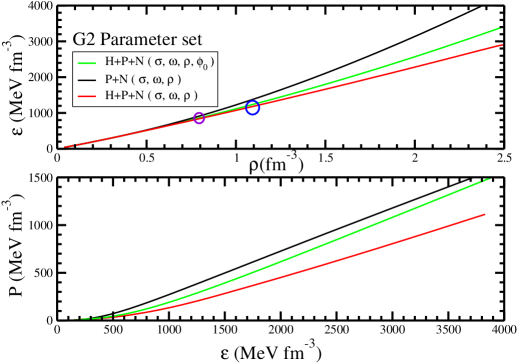
Figure 1: The upper panel of the graph shows the variation of the baryon density with energy density. The upper most curve gives the EOS for nucleonic matter (nucleon+lepton), the middle one indicates hyperonic (hyperon+lepton) matter with $\phi_{0}$-meson contribution. The lower one is same as middle one except contribution of $\phi_{0}$-meson. The lower panel of the graph shows the variation of the energy density with pressure density. G2 parameter set is used for these calculation.

2 Theoretical formalism

Relativistic mean filed model provides a smooth road to go from finite nuclear system to neutron star system, which has an extreme dense and high isospin asymmetry environment. Now-a-days RMF model is used to study various properties of the neutron and hyperon star. Starting point of the RMF model is an effective Lagrangian. For the present calculation, I use an effective Lagrangian which contains non-linear interactions of $\sigma$ and $\omega$-meson and cross-coupling of various effective mesons [26, 34, 28, 35] ,

$${\cal L}=\sum_{B}\overline{\psi}_{B}\bigg{(}i\gamma^{\mu}\partial_{\mu}-m_{B}+g_{\sigma B}\sigma-g_{\omega B}\gamma_{\mu}\omega^{\mu}-\frac{1}{2}g_{\rho B}\gamma_{\mu}\tau\rho^{\mu}-g_{\phi_{0}B}\gamma_{\mu}{\phi_{0}}^{\mu}\bigg{)}\psi_{B}+\frac{1}{2}\partial_{\mu}\sigma\partial_{\mu}\sigma$$

$$-m_{\sigma}^{2}\sigma^{2}\left(\frac{1}{2}+\frac{\kappa_{3}}{3!}\frac{g_{\sigma}\sigma}{m_{B}}+\frac{\kappa_{4}}{4!}\frac{g_{\sigma}^{2}\sigma^{2}}{m_{B}^{2}}\right)-\frac{1}{4}\Omega_{\mu\nu}\Omega^{\mu\nu}+\frac{1}{2}m_{\omega}^{2}\omega_{\mu}\omega^{\mu}\left(1+\eta_{1}\frac{g_{\sigma}\sigma}{m_{B}}+\frac{\eta_{2}}{2}\frac{g_{\sigma}^{2}\sigma^{2}}{m_{B}^{2}}\right)-\frac{1}{4}R_{\mu\nu}R^{\mu\nu}$$

$$+\frac{1}{2}m_{\rho}^{2}R_{\mu}R^{\mu}\left(1+\eta_{\rho}\frac{g_{\sigma}\sigma}{m_{B}}\right)+\frac{1}{4!}\zeta_{0}\left(g_{\omega}\omega_{\mu}\omega^{\mu}\right)^{2}+\frac{1}{2}{m_{\phi}}^{2}{\phi_{\mu}}{\phi^{\mu}}+\sum_{l}\overline{\psi}_{l}\left(i\gamma^{\mu}\partial_{\mu}-m_{l}\right)\psi_{l}+\Lambda_{v}R_{\mu}R^{\mu}(\omega_{\mu}\omega^{\mu}),$$ (1)

where $\omega_{\mu\nu}$ and $R_{\mu\nu}$ are field tensors for the $\omega$ and $\rho$ fields respectively and are defined as $\omega_{\mu\nu}=\partial_{\mu}\omega_{\nu}-\partial_{\nu}\omega_{\mu}$ and $R_{\mu\nu}=\partial_{\mu}R_{\nu}-\partial_{\nu}R_{\mu}$. The symbols are carrying their usual meanings. $\sigma$, $\omega$ and $\rho$-meson are exchanged between the nucleons, while $\phi_{0}$ being a strange meson it is exchanged between the hyperons only. The coupling constants of nucleon-meson interactions are fitted to reproduce the desired nuclear matter saturation properties and finite nuclear properties, like charge radius, binding energy, and monopole excitation energy of a set of spherical nuclei. The nature of the interaction depends on the quantum numbers and masses of the intermediate mesons. $\sigma$ (T=0, S=0) is an isoscalar-scalar meson, it gives intermediate attractive interaction. $\omega$-meson (T=0, S=1) is an isoscalar-vector meson, which gives short-range repulsive interaction. $\rho$-meson (T=1, S=1) is an isovector vector meson, whose interaction is account for the isospin asymmetry. Newly added $\phi_{0}$-meson is a vector meson, which gives similar interaction like $\omega$-meson [36, 37, 38, 39, 40, 41, 42]. By using classical Euler-Lagrangian equation of motion, we get the various equation of motions for the different mesons.

$$m_{\sigma}^{2}\left(\sigma_{0}+\frac{g_{\sigma N}\kappa_{3}\sigma_{0}}{2m_{B}}+\frac{\kappa_{4}g_{\sigma N}^{2}\sigma_{0}^{2}}{6m_{B}^{2}}\right)\sigma_{0}-\frac{1}{2}m_{\rho}^{2}\eta_{\rho}\frac{g_{\sigma N}\rho_{03}^{2}}{m_{B}}-\frac{1}{2}m_{\omega}^{2}\left(\eta_{1}\frac{g_{\sigma N}}{m_{B}}+\eta_{2}\frac{g_{\sigma N}^{2}\sigma_{0}}{m_{B}^{2}}\right)\omega_{0}^{2}=\sum g_{\sigma B}\rho^{s}_{B}.$$ (2)

$$m_{\omega}^{2}\left(1+\eta_{1}\frac{g_{\sigma N}\sigma_{0}}{m_{B}}+\frac{\eta_{2}}{2}\frac{g_{\sigma N}^{2}\sigma_{0}^{2}}{m_{B}^{2}}\right)\omega_{0}+\frac{1}{6}\zeta_{0}g_{\omega N}^{2}\omega_{0}^{3}=\sum g_{\omega B}\rho_{B}.$$ (3)

$$m_{\rho}^{2}\left(1+\eta_{\rho}\frac{g_{\sigma N}\sigma_{0}}{m_{B}}\right)R_{0}=\frac{1}{2}\sum g_{\rho B}\rho_{B3}.$$ (4)

$${m_{\phi}}^{2}\phi_{0}=\sum g_{\phi B}\rho_{B}.$$ (5)

Equation for the $\phi_{0}$-meson is similar to the $\omega$-meson except the coupling constants. We use the expression,

$$U_{Y}={m_{n}}(\frac{m_{n}^{*}}{m_{n}}-1)x_{\sigma Y}+(\frac{g_{\omega}}{m_{\omega}})^{2}\rho_{0}x_{\omega Y},$$ (6)

to calculate the hyperon potential depth. Y stands for the different hyperons ( $\Lambda,\Sigma,\Xi$ ). $x_{\sigma Y}$ and $x_{\omega Y}$ are the coupling constants of the hyperon-meson interactions and $\rho_{0}$ is the saturation density. We choose ${U_{\Lambda}}^{(N)}=-30$ MeV [46, 47], ${U_{\Sigma}}^{(N)}=+40$ MeV [48], and ${U_{\Xi}}^{(N)}=-28$ MeV [30]. The hyperon-meson coupling constants $x_{\sigma Y}$ and $x_{\omega Y}$ are fitted in a such a way that hyperon potential depth for various hyperons can be reproduced. We can vary the $x_{\sigma Y}$ and $x_{\omega Y}$ for different combinations to get the depth of the hyperon potentials. The hyperon interaction strengths with $\rho$-mesons are fitted according to the SU(6) symmetry [49], $x_{\Lambda\rho}=$ 0, $x_{\Sigma\rho}=$ 2, $x_{\Xi\rho}=$1. The interaction strengths of the hyperons with $\phi_{0}$-meson are given by $x_{\phi\Lambda}=$$-{\sqrt{2}}/{3}$ g_ωN, $x_{\phi\Sigma}=-{\sqrt{2}}/{3}$ $g_{\omega N}$, $x_{\phi\Xi}=-{2\sqrt{2}}/{3}$ $g_{\omega N}$. These equations form a set of self- consistent equations, which can be solved by iterative method to find various meson fields and densities. Using energy-momentum tensor, the total energy and pressure density can be written,

$${\cal E}=\sum_{B}\frac{Y_{B}}{(2\pi)^{3}}\int_{0}^{k_{F}^{B}}d^{3}k\sqrt{k^{2}+{m_{B}}^{*}}+m_{\sigma}^{2}\sigma_{0}^{2}\left(\frac{1}{2}+\frac{\kappa_{3}}{3!}\frac{g_{\sigma}\sigma_{0}}{m_{B}}+\frac{\kappa_{4}}{4!}\frac{g_{\sigma}^{2}\sigma_{0}^{2}}{m_{B}^{2}}\right)+\frac{1}{2}m_{\omega}^{2}\omega_{0}^{2}\left(1+\eta_{1}\frac{g_{\sigma}\sigma_{0}}{m_{B}}+\frac{\eta_{2}}{2}\frac{g_{\sigma}^{2}\sigma_{0}^{2}}{m_{B}^{2}}\right)$$

$$+\frac{1}{2}m_{\rho}^{2}\rho_{03}^{2}\left(1+\eta_{\rho}\frac{g_{\sigma}\sigma_{0}}{m_{B}}\right)+\frac{1}{2}{m_{\phi}}^{2}\phi^{2}+\frac{1}{8}\zeta_{0}g_{\omega}^{2}\omega_{0}^{4}+\sum_{l}\int_{0}^{k_{F}^{l}}\sqrt{k^{2}+{m_{l}}^{2}}k^{2}dk+3\Lambda_{V}\omega_{0}^{2}R_{0}^{2},$$ (7)

and

$${\cal P}=\sum_{B}\frac{Y_{B}}{3(2\pi)^{3}}\int_{0}^{k_{F}^{B}}\frac{k^{2}d^{3}k}{\sqrt{k^{2}+{m_{B}^{*}}^{2}}}-m_{\sigma}^{2}\sigma_{0}^{2}\left(\frac{1}{2}+\frac{\kappa_{3}}{3!}\frac{g_{\sigma}\sigma_{0}}{m_{B}}+\frac{\kappa_{4}}{4!}\frac{g_{\sigma}^{2}\sigma_{0}^{2}}{m_{B}^{2}}\right)+\frac{1}{2}m_{\omega}^{2}\omega_{0}^{2}\left(1+\eta_{1}\frac{g_{\sigma}\sigma_{0}}{m_{B}}+\frac{\eta_{2}}{2}\frac{g_{\sigma}^{2}\sigma_{0}^{2}}{m_{B}^{2}}\right)$$

$$+\frac{1}{2}m_{\rho}^{2}\rho_{03}^{2}\left(1+\eta_{\rho}\frac{g_{\sigma}\sigma_{0}}{m_{B}}\right)+\Lambda_{V}R_{0}^{2}\omega_{0}^{2}+\frac{1}{24}\zeta_{0}g_{\omega}^{2}\omega_{0}^{4}+\frac{1}{3\pi^{2}}\sum_{l}\int_{0}^{k_{F}^{l}}\frac{k^{4}dk}{\sqrt{k^{2}+m_{l}^{2}}},$$ (8)

where, $l$ stands for the leptons like electron and muon. Variation of total energy and pressure density with baryon density known as the equation of state of the nuclear matter. Putting $\beta$-equilibrium and charge neutrality conditions, it can be converted to the star matter equation of state. These equation of states are the inputs of the Tolman-Oppenheimer-Volkoff (TOV) [43, 44] equation, which is given by

$$\frac{\partial P}{\partial r}=-\frac{(P+\rho)(M(r)+4\pi r^{3}P)}{r(r-2m)},$$ (9)

$$\frac{\partial m}{\partial r}=4\pi r^{2}\rho(r),$$ (10)

where $m(r)$ is the enclosed gravitational mass, $P$ is the pressure, $\cal E$ is the total energy density and $r$ is the radial variable. These two coupled hydro-static equations are solved to get the mass and radius of the neutron star at a certain central density. Different central density gives different combination of mass and radius and one particular choice of central density gives maximum mass of the neutron star for a given EOS.

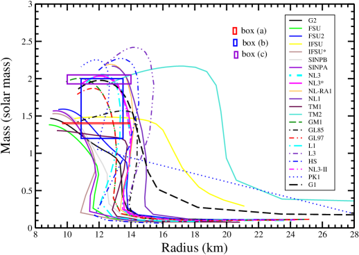
Figure 2: The figure shows the mass-radius curve for the various parameter sets of the RMF model. Box (a), shows acceptable range of the radius of canonical star (1.4$M_{\odot}$), while box (b) represents the star mass in the range 1.2–2 $M_{\odot}$ with radius 10.7–13.5 km. The box (c) shows the limit on the maximum mass of the neutron star ie. 1.93– 2.05 $M_{\odot}$.

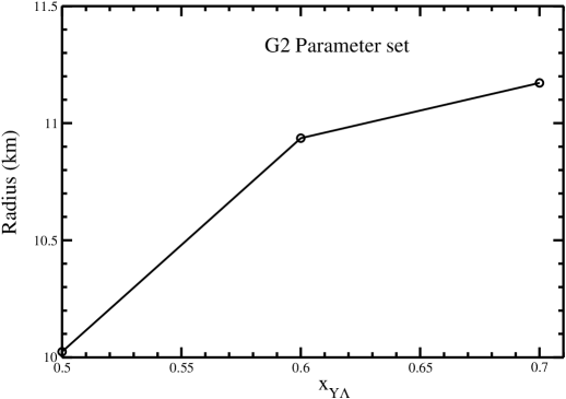
Figure 3: The graph shows the variation of the radius of the canonical star (1.4$M_{\odot}$) with hyperon-meson coupling constants $x_{\Lambda Y}$.

3 Results and discussions

In the present proceeding, I use 22 parameter sets of the RMF model to calculate the properties of the hyperon star. These parameter sets are divided into five groups according to the nature of the nucleon-nucleon interaction. The parameter sets belong to a same group are only different from each other by the value of the coupling constants and saturation properties. From example, group I, contain G1 and G2 parameter sets. Both G1 and G2 have a similar type of nucleon-meson interaction and contain the same cross-couplings and self-interactions among mesons. These 22 parameter sets are commonly used in RMF calculations. These parameter sets are differentiated from each other in a wide range of saturation properties like incompressibility (K), symmetry energy (J), saturation binding energy (E/A) and saturation density ($\rho_{0}$). These saturation properties also cover a wide range of value such as, incompressibility of NL1 is 211.4 MeV, while that of L1 is 626.3 MeV. Similarly, symmetry energy value ranges from 21.7 MeV (L1) to 43.7 MeV (NL1). These two quantities of nuclear matter affect the EOS of the neutron star in a significant way. The perspective of taking so many parameter sets is that to check the predictive capacity of RMF model with different parameter sets.

Nuclear matter equation of state is considered as one of the most important ingredient for the calculation of neutron star properties. Before the discussion the effects of the $\phi_{0}$-meson on the properties of the hyperon star, it is wise to investigate how the $\phi_{0}$-meson affects the EOS. In Fig. 1 the effects of $\phi_{0}$-meson on the EOS of neutron star matter are shown. The upper panel shows the variation of the baryon density with energy density. Upper curve of the upper panel is for the pure neutron-proton matter with no contribution of the hyperons. This curve is the stiffest one. The lowest curve contains the contribution of hyperon. The middle one contain contribution of the hyperon along with the $\phi_{0}$-meson as inter-mediating meson. The graph clearly shows the $\phi_{0}$-meson makes the EOS stiff. So it increases the maximum mass of the hyperon star. In the upper panel of the Fig. 1, contribution of the $\phi_{0}$-meson comes around 0.8 fm^-3, which is shown by a blue circle. So it makes the EOS with $\phi_{0}$ and without $\phi_{0}$-meson deviate from each other around 0.8 fm^-3. The lower panel shows the variation of the energy density with pressure density. The pressure-energy density graph also follows similar trend as in the upper panel. The hyperon star matter without $\phi_{0}$-meson shows a soft EOS, while with $\phi_{0}$-meson it shows a comparative stiff EOS. In Fig.2, I show the mass-radius graph with different parameter sets. Three boxes are shown in the figure. The box (a) represents the radius of the canonical star (1.4 $M_{\odot}$) [45]. From the study of chiral effective model, authors in Ref.[45] suggested that the radius of the canonical star lies in the range 9.7–13.9 km. The figure shows that most of the parameter sets are unable to reproduce the radius of the canonical star (1.4 $M_{\odot}$) in the above range. Only a few parameter sets lik FSU2, PK1, GL85, Gl97 , SINPA, SINPB, NL3, NL3*, IFSU*, and G2 can give the radius of the canonical star in the above range. But the radius of the canonical star depends on the hyperon-meson coupling constants. For example, if I change the hyperon-meson coupling constants , while keeping fix the different hyperon potential, the radius of the canonical star increases monotonically with hyperon-meson interaction strength. The box (b), shows the star with mass 1.2–2 $M_{\odot}$ and radius in the range 10.7–13.5 km. Many parameter sets are able to reproduce the mass and radius in this range. These parameter sets are GL97, GL85, FSU, TM1, PK1, GM1 SINPA, and SINPB. Simillarly, the box (c) indicates the limit of the maximum mass of the neutron star from recent observations. GM1, NL3-II, NL3, NL3*, parameter sets have maximum mass in this recent observation limit, which is 1.93–2.05 $M_{\odot}$. Fig.3, shows the variation of radius of the canonical star (1.4 $M_{\odot}$) with hyperon-meson coupling constants. For the quantitative check, $x_{\sigma\Lambda}$ changed from 0.5 to 0.7 as result the radius changed from 10.0278 km to 11.275 km. The radius of the canonical star changes to 13% by changing the hyperon-meson coupling constant to 0.2. While changing the $x_{\sigma\Lambda}$ values, we also keep changing the value of $x_{\omega\Lambda}$ to fix the value of the $U_{\Lambda}$ at -30 MeV. In the similar way, I take care the hyperon-meson coupling constants for other hyperons. I keep the potential of $U_{\Lambda}$, and $U_{\Sigma}$ and $U_{\Xi}$, while changing the $x_{\sigma Y}$ and $x_{\omega Y}$.

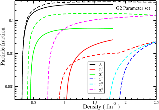
Figure 4: Particle fraction of the hyperon with G2 parameter set. The solid lines show the particle fraction of different types of hyperons with $\phi_{0}$-meson and the corresponding dotted lines show the result of hyperons without $\phi_{0}$-meson.

Fig.4, shows the effect of the $\phi_{0}$-meson on the hyperon production with G2 parameter set. The solid lines represent the hyperon production with $\phi_{0}$-meson contribution, while the dotted line without $\phi_{0}$-meson. This graph shows that $\phi_{0}$-meson shifts the threshold density (density at which different hyperons are produced) to higher density. For example, without the contribution of the $\phi_{0}$-meson the $\Xi$ produces at a density 0.3989 fm ^-3, but the addition of $\phi_{0}$-meson shifts the threshold density to 0.461 fm^-3. Similarly, $\Sigma^{+}$ hyperon’s threshold density shifts from 0.914 fm^-3 to 1.038 fm^-3. The threshold density of the $\Lambda$-hyperon does not shift by a significant amount. In the table 1, the maximum mass, the corresponding radius, compactness, and the central density at which maximum mass occurs for the hyperon star are given with different parameter sets. Results are given for the neutron star, hyperon star with $\sigma$-$\omega$-$\rho$-model and hyperon star with $\sigma$-$\omega$-$\rho$-$\phi_{0}$-model. We conclude from the table 1, for all the parameter sets the maximum masses follow a general trend i.e. $M_{\mathrm{max}}^{N}$ ($\sigma$-$\omega$-$\rho$) $>$ $M_{\mathrm{max}}^{H}$ ($\sigma$-$\omega$-$\rho$-$\phi_{0}$) $>$ $M_{\mathrm{max}}^{H}$ ($\sigma$-$\omega$-$\rho$), where $M_{\mathrm{max}}^{N}$ ($\sigma$-$\omega$-$\rho$) is the maximum mass of the proton-neutron star in $\sigma$-$\omega$-$\rho$ model and $M_{\mathrm{max}}^{H}$ ($\sigma$-$\omega$-$\rho$-$\phi_{0}$) is the maximum mass of the hyperon star in $\sigma$-$\omega$-$\rho$-$\phi_{0}$ model. But the radius does not follows any common trend in all parameter sets. The compactness (M/R) also follows a general trend i.e. $(M/R)^{N}$ ($\sigma$-$\omega$-$\rho$) $>$ $(M/R)^{H}$ ($\sigma$-$\omega$-$\rho$-$\phi_{0}$) $>$ $(M/R)^{H}$ ($\sigma$-$\omega$-$\rho$) for all the parameter sets. The data shows by adding the $\phi_{0}$-meson the compactness of the hyperon star increases, this is mainly due to the increse of the maximum mass with the inclusion of $\phi_{0}$-meson. The central density (${\cal E}_{c}$) at which the maximum mass occurs, also follows a common pattern for all the parameter sets i.e. ${\cal E}_{c}^{N}$ ($\sigma$-$\omega$-$\rho$) $<$ ${\cal E}_{c}^{H}$ ($\sigma$-$\omega$-$\rho$-$\phi_{0}$) $<$ ${\cal E}_{c}^{H}$ ($\sigma$-$\omega$-$\rho$).

Table 1: Maximum mass (M), corresponding radius at maximum mass (R), compactness (M/R), and central density (${\cal E}_{c}$) for the neutron and hyperon stars are given with various parameter sets.

	Neutron star				Hyperon star with $\phi_{0}$				Hyperon star without $\phi_{0}$
parameter	M	R	M/R	${\cal E}_{c}\times 10^{15}$	M	R	M/R	${\cal E}_{c}\times 10^{15}$	M	R	M/R	${\cal E}_{c}\times 10^{15}$
sets	($M_{\odot}$)	(km)	($M_{\odot}$/km)	( g cm-3)	($M_{\odot}$)	(km)	($M_{\odot}$/km)	( g cm-3)	($M_{\odot}$)	(km)	($M_{\odot}$/km)	(g cm-3)
GROUP I
G2	1.938	11.126	0.174	2.317	1.576	9.622	0.163	3.387	1.299	9.054	0.135	3.921
G1	2.162	12.244	0.176	1.871	1.881	11.712	0.160	2.139	1.816	12.048	0.150	1.960
GROUP II
FSU	1.722	10.654	0.161	2.495	1.419	9.280	0.152	3.743	1.100	8.788	0.125	3.921
FSU2	2.072	12.036	0.172	1.960	1.779	11.399	0.155	2.139	1.377	10.812	0.127	2.674
IFSU	1.898	12.612	0.150	1.960	1.793	13.450	0.133	1.604	1.750	13.890	0.125	1.426
IFSU*	1.985	11.386	0.174	1.529	1.763	10.90	0.161	2.317	1.570	10.820	0.145	2.317
SINPA	2.001	11.350	0.176	2.139	1.750	10.652	0.164	2.495	1.525	10.334	0.147	2.674
SINPB	1.994	11.468	0.173	2.139	1.719	10.536	0.163	2.674	1.404	10.258	0.136	2.674
GROUP III
TM1	2.176	12.236	0.177	1.871	1.966	11.986	0.164	1.960	1.798	12.228	0.1470	1.782
TM2	2.622	16.508	0.158	1.069	2.512	17.062	0.147	0.944	2.479	17.358	0.142	0.929
PK1	2.489	14.042	0.177	1.604	2.275	13.688	0.166	1.782	2.128	13.904	0.153	1.782
GROUP IV
NL3	2.774	13.154	0.210	1.604	2.633	13.012	0.193	1.604	2.529	13.012	0.194	1.6044
NL3*	2.760	13.102	0.210	1.604	2.605	12.938	0.201	1.604	2.500	12.930	0.193	1.604
NL1	2.844	13.630	0.208	1.426	2.653	13.740	0.193	1.604	2.506	13.190	0.189	1.604
GM1	2.370	12.012	0.197	1.960	2.280	12.14	0.187	1.871	2.230	12.21	0.182	1.77
GL85	2.168	12.092	0.220	1.960	2.122	12.242	0.173	1.871	2.106	12.223	0.172	1.871
GL97	2.003	10.790	0.185	2.495	1.919	10.832	2.495	0.177	1.881	10.894	0.172	2.495
NL3-II	2.774	13.146	0.211	1.604	2.594	12.94	0.200	1.604	2.474	12.742	0.194	1.782
NL-RA1	2.783	13.420	0.207	1.426	2.631	13.050	0.201	1.604	2.516	13.030	0.193	1.604
GROUP V
HS	2.974	14.176	0.209	1.2478	2.853	13.848	0.206	1.4261	2.770	13.860	0.199	1.426
L1	2.744	13.004	0.211	1.604	2.056	12.176	0.168	1.871	2.00	12.372	0.161	1.786
L3	3.186	15.224	0.209	1.069	2.088	12.374	0.168	1.782	1.692	12.294	0.137	1.069

4 Summary and Conclusions

In summary, I study the properties of the hyperon stars with the various parameter sets of RMF model. The predictive capacity of the various parameter sets to reproduce the canonical mass-radius relationship are discussed with hyperonic degrees of freedom. Out of 22 parameter sets only few parameter sets like FSU2, PK1, GL85, Gl97 , SINPA, SINPB, NL3, NL3*, IFSU*, and G2 can able to reproduce the radius of the canonical star (1.4 $M_{\odot}$) in the range 9.7 km to 13.9 km. But radius of 1.4 $M_{\odot}$ star depends on the strongly on the hyperon-meson couplings. The radius of a canonical star increases monotonically with hyperon-meson interaction in-spite of a fixed hyperon potential depth. The radius of a canonical star change by 13% with a small change of 0.2 of the hyperon-meson coupling constants. This shows not only the depth of the hyperon potential but also the range of the hyperon-meson coupling constants are improtant. More hyper-nuclei data required to fix the range of the hyperon-hyperon interaction. As the $\phi_{0}$ is a vector meson, so it gives repulsive interaction among the hyperons and makes the EOS comparatively stiff The stiff EOS increases the maximum mass of the hyperon star. The compactness of the hyperon star increases with inclusion of the $\phi_{0}$-meson. The $\phi_{0}$-meson push the threshold density of hyperon production to higher density.

5 Acknowledgement

All the calculations are preformed in Institute of Theoretical Physics, Chinese Academy of Sciences. This work has been supported by the National Key R&D Program of China (2018YFA0404402), the NSF of China (11525524, 11621131001, 11647601, 11747601, and 11711540016), the CAS Key research Program (QYZDB-SSWSYS013 and XDPB09), and the IAEA CRP ”F41033”.

References

- [1] G. Baym and C. Pethick, Annu. Rev. of Astron. and Astrophys., 17, 415 (1979).
- [2] J. M. Lattimer, Science, 304, 536 (2004).
- [3] J. Antoniadis et. al, Science, 340, 6131 (2013).
- [4] Clifford E. Rhoades and Remo Ruffini, Phys. Rev. Lett., 32, 324 (1974).
- [5] J. M. Weisberg and J. H. Taylor, http://arxiv.org/abs/astro-ph/0211217v1,
- [6] J. G. Martinez and K. Stovall and P. C. C. Freire and J. S. Deneva and F. A. Jenet and M. A. McLaughlin and M. Bagchi and S. D. Bates and A. Ridolfi, The Astrophysical Journal, 812, 143 (2015).
- [7] N. K. Glendenning, Astrophys. J., 293, 470 (1985).
- [8] P. B. Demorest and T. Pennucci and S. M. Ransom and M. S. E. Roberts and J. W. T. Hessels, Nature, 467, 1081 (2010).
- [9] Paulo C. C. Freire and Alex Wolszczan and Maureen van den Berg and Jason W. T. Hessels, Astrophys. J., 679, (2008).
- [10] V. A. Ambartsumyan and G. S. Saakyan, Sov. Astron., 4, 187 1960.
- [11] S. Weissenborn, D. Chatterjee, and J. Schaffner-Bielich, Phys. Rev. C, 85, 065802 (2012).
- [12] S. Weissenborn, D. Chatterjee, and J. Schaffner-Bielich, Phys. Rev. C 90, 019904 (2014).
- [13] M Oertel and C Providência and F Gulminelli and Ad R Raduta, J. Phys. G: Nucl. Part. Phys., 42, 075202 (2015).
- [14] I. Vidaña and D. Logoteta and C. Providência and A. Polls and I. Bombaci, Europhys. Lett., 94, 11002 (2011).
- [15] Y. Yamamoto, T. Furumoto, N. Yasutake, and Th. A. Rijken, Phys. Rev. C, 88, 022801 (2013).
- [16] Feryal Özel and Dimitrios Psaltis and Scott Ransom and Paul Demorest and Mark Alford, Astrophys. J. Lett., 724, L199 (2010).
- [17] L. Bonanno, and A. Sedrakian, Astron. and Astrophys., 539, A16 (2012).
- [18] R. J. Furnstahl, Brian D. Serot, and Hua-Bin Tang, Nucl. Phys. A, 615, 441 (1997).
- [19] F. J. Fattoyev, and J. Piekarewicz, Phys. Rev. C, 82, 025805, (2010).
- [20] B. G. Todd-Rutel, and J. Piekarewicz, Phys. Rev. Lett., 95, 122501 (2005).
- [21] Wei-Chia Chen, and J. Piekarewicz, Phys. Rev. C, 90, 044305 (2014).
- [22] Y. Sugahara and H. Toki, Nucl. Phys. A, 579, 557 (1994).
- [23] Wenhui Long, Jie Meng, Nguyen Van Giai, and Shan-Gui Zhou, Phys. Rev. C, 69, 034319, (2004).
- [24] G. A. Lalazissis, J. König, and P. Ring, Phys. Rev. C, 55, 540 (1997).
- [25] G. A. Lalazissis, S. Karatzikos, R. Fossion, and D. P. Arteaga, , A. V. Afanasjev, and P. Ring, Phys. Lett. B, 671, 36 (2009).
- [26] P. G. Reinhard, M. Rufa, J. Maruhn, W. Greiner, and J. Friedrich, Z. Phys. A Atomic Nuclei, 323, 13 (1986).
- [27] M. Rashdan, Phys. Rev. C, 63, 044303 (2001).
- [28] R. J. Furnstahl, C. E. Price and G. E. Walker, Phys. Rev. C 36, 2590 (1987).
- [29] C. Mondal, B. K. Agrawal, J. N. De, and S. K. Samaddar, Phys. Rev. C, 93, 044328 (2016).
- [30] N. K. Glendenning, and S. A. Moszkowski, Phys. Rev. Lett., 67, 2414 (1991).
- [31] N. K. Glendenning, Compact Stars : Nuclear Physics, particle Physics , and General Relativity, (1997).
- [32] J. D Walecka, Ann. Phys., 83, 491 (1974).
- [33] C. J. Horowitz, and B. D. Serot, Nucl. Phys. A, 368, 503 (1981).
- [34] L. D. Miller, A. E. S. Green, Phys. ReV. C, 5, 241 (1972).
- [35] P. Ring, Prog. Part. Nucl. Phys., 37, 193 (1996).
- [36] Rafael Cavagnoli and Debora P Menezes, J. Phys. G: Nucl. Part. Phys., 35 115202 (2008).
- [37] Bipasha Bhowmick, Madhubrata Bhattacharya, Abhijit Bhattacharyya, and G. Gangopadhyay, Phys. Rev. C, 89, 065806 (2014).
- [38] I. Bednarek, M. Keska, and R. Manka, Phys. Rev. C, 68, 035805 (2003).
- [39] S. Pal, M. Hanauske, I. Zakout, H. Stöcker, and W. Greiner, Phys. Rev. C, 60, 015802 (1999).
- [40] J. K. Bunta and S. Gmuca, Phys. Rev. C, 70, 054309 (2004).
- [41] J. Schaffner, and I. N. Mishustin, Phys. Rev. C, 53, (1996).
- [42] Xian-Feng Zhao, Phys. Rev. C, 92, 055802, (2015).
- [43] R. C. Tolman, Phys. ReV. 55, 364 (1939).
- [44] J. R. Oppenheimer and G. M. Volkoff, Phys. ReV. 55, 374 (1939).
- [45] K. Hebeler and J. M. Lattimer and C. J. Pethick and A. Schwenk, Phys. Rev. Lett. 105, 161102 (2010).
- [46] C.J. Batty and E. Friedman and A. Gal, Phys. Rep., 287 385 (1997).
- [47] D. J. Millener, C. B. Dover and A. Gal, Phys. Rev. C 38, 2700 (1988).
- [48] E. Friedman and A. Gal, Phys. Rep., 452 89 (2007).
- [49] C.B. Dover and A. Gal, Prog. Part. Nucl. Phys., 12, 171 (1984).