Equal Opportunity and Affirmative Action
via
Counterfactual Predictions
Abstract
Machine learning (ml) can automate decision-making by learning to predict decisions from historical data. However, these predictors may inherit discriminatory policies from past decisions and reproduce unfair decisions. In this paper, we propose two algorithms that adjust fitted ml predictors to make them fair. We focus on two legal notions of fairness: (a) providing equal opportunities (eo) to individuals regardless of sensitive attributes and (b) repairing historical disadvantages through affirmative action (aa). More technically, we produce fair eo and aa predictors by positing a causal model and considering counterfactual decisions. We prove that the resulting predictors are theoretically optimal in predictive performance while satisfying fairness. We evaluate the algorithms, and the trade-offs between accuracy and fairness, on datasets about admissions, income, credit, and recidivism.
1 Introduction
Machine learning (ml) methods can automate costly decisions by learning from historical data. For example, ml algorithms can assess the risk of recidivism to decide bail releases or predict admissions to determine which college applicants should be further reviewed (waters2014grade).
Consider an admissions committee that decides which applicants to accept to a university. Given historical data about the applicants and the admission decisions, an ml algorithm can learn to predict who will be admitted and who will not. The ml predictor might accurately simulate the committee’s decisions, but it might also inherit some of the undesirable properties of the committee. If the committee was systematically and unfairly biased then its ml replacement will be biased as well.
In this paper, we develop algorithms for learning ml predictors that are both accurate and fair. Our methods maintain as much fidelity as possible to the decisions of the committee, but they adjust the predictor to ensure that the algorithmic decisions are fair.
We focus on two legal notions of fairness: equal opportunities (eo) and affirmative action (aa). An eo decision provides the same opportunities to similar candidates with different backgrounds (barocas2016big). In admissions, for example, an eo decision admits applicants based only on their qualifications; applicants with the same merit, such as a test score, should have the same chance of admission regardless of their race or sex.
Some applicants might have lower test scores only because they belong to a historically disadvantaged demographic group, one that has less access to opportunities. The legal notion of affirmative action (aa) acknowledges these historical disadvantages (anderson2002integration). For example, aa will correct for situations where male applicants have easier access to extra test preparation. (Notice that, by definition, an aa decision is not an eo decision because aa decisions provide advantages based on group membership.)
Using these two notions of fairness, we develop algorithms that adjust ml predictors to be fair predictors. The first produces algorithmic decisions that ensure equal opportunities for disadvantaged groups; the second produces decisions that exercise affirmative action to repair existing disparities. We prove the algorithms are theoretically optimal—they provide as good predictions as possible while still being fair.
In detail, we use ideas from causal machine learning (pearl2009causality; peters2017elements). First we posit a causal model of the historical decision-making process. In that model, the decision can be affected by all the attributes, both sensitive and non-sensitive, and the sensitive attributes can also affect the non-sensitive ones (e.g., sex can affect test scores). Then we consider algorithmic decisions as causal variables, ones whose values are functions of the attributes. Once framed this way, we can ask counterfactual questions about an algorithm, e.g., “what would the algorithm decide for this applicant if she had achieved the same test score but was a male?” We operationalize eo and aa fairness as probabilistic properties of such counterfactual decisions. (aa-fairness is the same as counterfactual fairness, proposed in kusner2017counterfactual.) Finally, we derive a method that adjusts a classical ml decision-maker to be eo-fair, and that adjusts an eo decision-maker to exercise aa.
We study our algorithms on simulated admissions data and on three public datasets, about income, credit, and recidivism. We examine the gap in accuracy between classical prediction and eo/aa-fair prediction, and we investigate the degree of unfairness that classical prediction would exhibit. Compared to other approaches to eo/aa-fairness, ours provide higher accuracy while remaining fair.
Related Work. Several threads of related work draw on causal models to formalize fairness. kilbertus2017avoiding relate paths and variables in causal models to violations of eo and aa. zhang2018fairness decompose existing fairness measures into discrimination along different paths in the causal graph, and propose fair decision algorithms that satisfy the path-specific criteria. kusner2017counterfactual introduce counterfactual fairness and an algorithm to satisfy it. Our work also uses causal graphs to formalize the eo and aa criteria, but our fair algorithms are designed to minimally correct fitted ml predictors. Like FairLearning kusner2017counterfactual, our aa-fair algorithm also satisfies counterfactual fairness, but our algorithm has higher fidelity to the historical decisions.
Other research has proposed a variety of statistical definitions of fairness for supervised learning (hashimoto2018fairness; chen2019fairness; kleinberg2016inherent; chouldechova2017fair; zafar2017fairness). hardt2016equality and kallus2018residual show, however, that these approaches cannot distinguish between different mechanisms of discrimination and they are not robust to changes in the data distribution. By building on causal machine learning, our work separates direct discrimination from indirect bias, and it is robust to changes in the data distribution.
Another line of work focuses on data preprocessing. zemel2013learning learn intermediate representations that remove information about the sensitive attributes; calders2010three and kamiran2012data reweight training data to control false positive/negative rates. In contrast, our eo-fair and aa-fair algorithms adjust ml predictions without changing the training data.
wang2019repairing modify black-box ml predictors to correct for historical disadvantages, as in aa. They define adjusted distributions over attributes for the disadvantaged group and solve optimal transport problems to repair predictors. Our predictors also minimally adjust ml predictors but we derive adjustments using causality.
Finally, dwork2012fairness define individual fairness, which formalizes eo without causality. Given a distance metric between individuals, it requires that similar individuals receive similar decisions. Our eo-fair algorithm recovers this requirement without relying on an explicit distance metric, which can be difficult to construct. dwork2012fairness also specify group-level aa fairness as independence between the sensitive attribute and decision (demographic parity). We exercise aa for each individual while also satisfying demographic parity.
Contributions. We develop optimal eo and aa algorithms. These algorithms modify existing ml predictors to produce eo-fair and aa-fair decisions, and we prove these decisions maximally recover the ml predictors under the fairness constraints. While existing approaches must omit descendants of the sensitive attributes to construct aa-fair decisions (kusner2017counterfactual; kilbertus2017avoiding), our aa algorithm uses all available attributes and is still aa-fair. Empirically, we show that our eo and aa algorithms produce better decisions than existing approaches that satisfy the same fairness criteria.
2 Assessing fairness with counterfactuals
| ID | Sex | Test | Admit | |||
| 1 | f | 54 | yes | |||
| 2 | m | 66 | no | |||
| ⋮ | ⋮ | ⋮ | ⋮ | |||
| 5000 | f | 44 | no | |||
| A | f | 85 | ? | 0.67 | 0.77 | 0.78 |
| B | m | 85 | ? | 0.84 | 0.77 | 0.76 |
| C | f | 65 | ? | 0.57 | 0.69 | 0.70 |
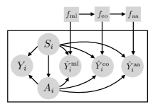
As a running example, consider automating the admissions process at a university. Using a dataset of past admissions, the goal is to algorithmically compute the admissions decision for new applicants. The dataset contains applicants and the committee’s decision about whether to admit them. Each applicant has demographic attributes, such as sex, religion, or ethnicity, that the university has deemed sensitive. Each applicant also has other attributes, such as a standardized test score or grade point average, that are not sensitive.
For simplicity, suppose each applicant has two attributes, their sex and their score on a standardized test. The sex of the applicant is a sensitive attribute; the test score is not. (Our algorithms extend to multiple attributes but this simple case illustrates the concepts.) Fig. 2 shows an example of such data.
We will use a causal model of this decision-making process to define two notions of fairness.
A causal model of the decision. First posit a causal model of the admissions process, such as the causal graph in Fig. 2. It assumes that an applicant’s sex and test score affect the admissions decision . For example, the admissions committee might unfairly prefer to admit males. The model also assumes the applicant’s sex can affect the test score. For example, female applicants might receive less exposure to test preparation, a disparity that results in lower scores.111We acknowledge these assumptions might be debatable; it is up to the user of our method to posit a sensible causal model of the historical decision process. (This simple model illustrates the core ideas; § 3 discusses extensions to more complicated causal graphs.)
The data in Fig. 2 matches the assumptions. It comes from the following structural model,
| (1) | ||||
(We threshold the test score to mimic real-world test scores that are usually bounded.) We set and so that for the same test score the committee is more likely to admit males than females. Moreover, we set to model that females perform less well on the test.
With data like Fig. 2 and a causal model, we can estimate the parameters of the functions that govern each variable in Fig. 2. (This estimation makes the usual assumptions about causal estimation, i.e., no open backdoor paths (pearl2009causality).)
The causal model implies counterfactuals, how the distribution of a variable changes when we intervene on others. For example, we can consider the counterfactual decision of a female applicant had she been a male. 222Even when sensitive attributes are immutable, we can define hypothetical interventions to articulate the counterfactuals (greiner2011causal). In this example, ”intervening on sex” means to make a person born of a different sex. Denote to be the counterfactual decision of the th applicant when we set their test score to be and sex to be .
Marginal distributions of counterfactuals provide an alternative to the do notation, . But counterfactual distributions can also be more complex: for example, is the probability of applicant ’s counterfactual admission if he was female, given that he is (factually) male and was admitted. See Ch. 7 of pearl2009causality for a treatment of how causal models imply distributions of counterfactuals.
We use counterfactual distributions to assess the fairness of decisions, either those made by the committee or those produced by an algorithm. We next describe the counterfactual criteria of equal opportunities and affirmative action.
Equal opportunities and its counterfactual criterion. A decision satisfies eo if changing the sensitive attribute does not change the distribution of the decision . Consider an applicant with sex and test score . An eo decision gives the same probability of admission even when changing the sex to (but keeping the test score at ). In Fig. 2, candidates A and B have the same test score but different sex; they should receive the same probability of admission.
Definition 1 (The eo criterion).
A decision satisfies equal opportunities (eo) in the sensitive attribute if
| (2) | ||||
for all and , where and are the domains of and .333Two random variables are equal in distribution if they have the same distribution function: for all .
The eo criterion differs from counterfactual fairness (kusner2017counterfactual). eo focuses on the counterfactual prediction had the applicant had the same non-sensitive attribute but a different sensitive attribute ; counterfactual fairness does not hold the attribute fixed.
The eo criterion also differs from equalized odds (hardt2016equality). Equalized odds requires the sensitive attribute to depend on the decision only via its ability to predict desirable downstream outcomes (e.g., college success). Equalized odds enforces statistical properties while eo assesses counterfactuals. The eo criterion assumes that the sensitive attribute does not causally affect the decision . (We prove this in Appendix A.)
Affirmative action and its counterfactual criterion. Affirmative action (aa) aims to correct for the historical disadvantages that may be caused by sensitive attributes. For example, female applicants may have had fewer opportunities for extracurricular test preparation, which leads to lower test scores and a lower likelihood of admission. Had they been male, they may have had more opportunities for preparation, achieved a higher score, and been admitted.
The goal of aa is to ensure that, all else being equal (e.g., effort or aptitude), an applicant would receive the same decision had they not been in a disadvantaged group. This is different from eo because it accounts for how the sensitive attribute affects the other attributes, for example how an applicant’s sex affects their test score.
The aa criterion requires that changing the sensitive attribute , along with the resulting change in the attribute , does not change the distribution of the decision . Consider an applicant with test score and sex . Had they belonged to a different group , they may have achieved a different test score . The aa criterion requires the counterfactual decision with the alternate sex to have the same distribution as the decision with the current sex . It was first proposed by kusner2017counterfactual, who dubbed it counterfactual fairness.
Definition 2 (The aa criterion, counterfactual fairness (kusner2017counterfactual)).
A decision satisfies affirmative action (aa) if
| (3) | ||||
for all . The random variable is the counterfactual of under intervention of the sensitive attribute .
In Eq. 3 the counterfactual attribute depends on the attributes of the applicant, . The variable captures, for example, that female applicants with high test scores will have even higher test scores had they been male. Assuming the causal model in Fig. 2, the aa criterion implies demographic parity (dwork2012fairness; kusner2017counterfactual), which requires the decision be independent of the sensitive attribute. We note that a decision cannot be both eo-fair and aa-fair.
Disparate treatment and impact. We have described two counterfactual criteria for fairness. One view on fairness is to seek to avoid “disparate treatment” or “disparate impact.” Applicants face disparate treatment when they are rejected by the biased admissions committee because of their sex. Applicants face disparate impact when they are systematically disadvantaged because they do not have the same opportunities for test preparation. From this perspective on fairness, an eo-fair decision eliminates disparate treatment; an aa-fair decision addresses disparate impact.
3 Constructing fair algorithmic decisions
Footnotes 3 and 2 define fairness in terms of distributions of counterfactual decisions. Using the causal model of the decision-making process, these definitions help evaluate the fairness of its outcomes. The criteria can assess any decisions, including those produced by a real-world process, such as an admissions committee, or those produced by an algorithm, such as a fitted ml model.
Consider a classical ml model that was fit to emulate historical admissions data; if the historical decisions are not eo or aa then neither will be the ml decisions. To this end, we develop fair ml predictors, those that are accurate with respect to historical data and produce eo-fair or aa-fair decisions. The key idea is to treat the algorithmic decision as another causal variable in the model and then to analyze its fairness properties in terms of the corresponding counterfactuals. We will show how to adjust decisions made by an ml model to make them eo-fair or aa-fair.
Formally, we use the language of decisions and predictors. Denote an algorithmic decision as , a causal variable that depends on the attributes . It comes from a fitted probabilistic predictor, , where is a probability density function. For example, an admissions decision is drawn from a Bernoulli that depends on the attributes (e.g., a logistic regression). By considering algorithmic decisions in the causal model, we can infer algorithmic counterfactuals and assess whether they satisfy the fairness criteria of § 2.
ml decisions. Consider a classical machine learning predictor, one that is fit to accurately predict the decision from and . In the admissions example, a binary decision, logistic regression is a common choice. The predictor draws the decision from a Bernoulli,
and the coefficients are fit to maximize the likelihood of the observed data. When incorporated into the causal model, and are illustrated in Fig. 2.
The ml decision will accurately mimic the historical data. However, it will also replicate harmful discriminatory practices. The decision might violate eo and not give equal opportunities to applicants of different sex. Nor will exercise aa. If policy mandates that admissions correct for the disparate impact of sex on the test score, then the ml decision cannot be used.
Return to the illustrative simulation in Fig. 2. We fit a logistic regression to the training data, which finds coefficients close to the mechanism that generated the data. Consequently, when used to form algorithmic decisions, it replicates the unfair committee. To see this, consider female applicant A and male applicant B and the classical ml decisions for each. For A, her probability of being admitted is . For B, his probability of admission is . Despite their identical test scores, the female applicant is less likely to get in.
ml decisions that satisfy equal opportunities. We use the ml predictor to produce an eo predictor , one whose decisions satisfy the eo criterion. Consider an ml predictor and an applicant with attributes . Their eo decision is , where
| (4) |
The distribution is the population distribution of the sensitive attribute.
The eo decision probability holds the non-sensitive attribute fixed, and takes a weighted average of the ml predictor for the sensitive attribute . Note all of its ingredients are computable: the distribution is estimated from the data and is the fitted ml predictor.
The eo decision satisfies Footnote 3: applicants with the same test score will have the same chance of admissions regardless of their sex. Further, it is the most accurate among all eo-fair decisions. We prove that it is eo-fair and minimally corrects ..
Theorem 1 (eo-fairness and optimality of eo decisions).
The decision is eo-fair. Moreover, among all eo-fair decisions, maximally recovers the ML decision ,
where is the set of eo-fair decisions. (The proof is in Appendix A.)
The intuition is that the eo decision preserves the causal relationship between the test score and the ml decision , but it ignores the possible effect of the sensitive attribute . In the do notation, what this means is that for all . Eq. 4 is the adjustment formula in pearl2009causality, which calculates .
Again return to Fig. 2. We use the fitted logistic regression to produce the eo predictor. This data has equal numbers of women and men, so the weighted average is
Using eo-fair decisions, applicants A and B both have a probability of admission.
Why not use fairness through unawareness (ftu) (kusner2017counterfactual)? ftu satisfies eo by fitting an ml model from the non-sensitive attribute to the decision . ftu decisions are also eo-fair; the sensitive attribute is never used. However, Theorem 1 states that the eo decisions of Eq. 4 are more accurate than ftu while still being eo-fair. We show this fact empirically in § 4.
ml decisions that exercise affirmative action. How can we construct an algorithmic decision that exercises affirmative action (aa)? We now show how to correct the eo-fair predictor to account for historical disadvantages that stem from the sensitive attribute .
Consider the eo-fair predictor and an applicant with attributes . Their aa-fair decision is , where
| (5) |
The distribution is the population distribution of the sensitive attribute; the distribution is the counterfactual distribution of the non-sensitive attribute , under intervention of and conditional on the observed values and .
This predictor exercises affirmative action because it corrects the applicant’s test score (and their resulting admissions decision) to their counterfactual test scores under intervention of the sex. Further, each element is computable from the dataset. (See below.) Note that aa-fair decisions can be formed from any eo-fair predictor.
One way to form an aa-fair decision is to draw from the mixture defined in Eq. 5. Consider the admissions example and an applicant : (a) sample a sex from the population distribution ; (b) sample a test score from its counterfactual distribution ; (c) sample the eo-fair decision for that counterfactual test score .
One subtlety of is in step (b): it draws the counterfactual test score under an intervened sex , but conditional on the observed sex and test score. This is an abduction—if a female applicant has a high test score , then her counterfactual test score will be even higher, and the likelihood of admission goes up beyond the eo-fair decision (pearl2009causality).
Put differently, the aa-fair predictor uses the eo-fair predictor , which only depends on the test score (and averages over the sex). However, the aa-fair predictor also corrects for the bias in the test score due to the sex of the applicant. It replaces the current test score with the adjusted score under . With this corrected score, it produces an aa-fair decision.
The aa-fair predictor depends on the sensitive attribute, and thus the aa-fair decision is not eo-fair: its likelihood changes based on the sex of the applicant. But among all aa-fair decisions, it is closest to the eo-fair decision. The following theorem establishes the theoretical properties of .
Theorem 2 (aa-fairness and optimality of the aa decisions ).
The decision is aa-fair. Moreover, among all aa decisions, the aa predictor minimally modifies the marginal distribution of ,
where are all aa decisions. It also preserves the marginal distribution of the eo predictor, . (The proof is in Appendix B.)
In Theorem 2, we also prove that aa-fair decisions preserve the marginal distribution of the eo-fair decisions. This property makes the aa predictor applicable as a decision policy. If the eo-fair predictor admits 20% of the applicants, the aa-fair predictor will also admit 20%. We need not worry that we admit more applicants than we can.
To finish the running example in Fig. 2, we exercise aa and calculate from . This is the predictor that requires abduction, calculating the test score that the applicant would have gotten had their sex been different. Consider applicant C. Her eo-fair probability of acceptance is , but when exercising aa it increases to . This adjustment corrects for the (simulated) systemic difficulty of females to receive test preparation and, consequently, higher scores.
Calculating eo and aa predictors. Alg. 1 provides the algorithm for calculating eo and aa predictors. (We prove its correctness in Appendix C.) The eo predictor adjusts the ML predictor ; it uses the ML predictor, but marginalizes out the sensitive attribute. The aa predictor adjusts the eo predictor ; it uses an abduction step (pearl2009causality) to impute from the model and its residual . In admissions, for example, the abduction step infers what a female applicant’s test score would have been if she had been male, given the score that she did achieve.
Alg. 1 differs from existing eo and aa algorithms in that it uses all available attributes. Recent works like kusner2017counterfactual and kilbertus2017avoiding avoid using descendants of the sensitive attributes to construct aa-fair decisions. FairLearning (kusner2017counterfactual) performs the same abduction step as to compute residuals but then fits a predictor using only the residuals and non-descendants of the sensitive attributes. For example, in admissions, after calculating the residual it does not include the test score in its predictor. In contrast, Alg. 1 uses all available attributes and still is aa-fair. The eo predictor in Alg. 1 also makes use of all attributes; it does not omit sensitive attributes as done in ftu (kusner2017counterfactual). In § 4 we demonstrate empirically that Alg. 1 forms more accurate decisions than these existing eo and aa algorithms.
Multiple sensitive attributes and general causal graphs. The admissions example involves one sensitive attribute, one non-sensitive attribute, and a binary decision. However, eo-fair and aa-fair decisions directly apply to cases with multiple sensitive (and non-sensitive) attributes, non-binary decisions, and more general causal structures.
Notably, aa-fair decisions can correct for bias when an individual belongs to an advantaged group in one sensitive attribute and a disadvantaged one in another. Consider both race and gender as sensitive attributes. If an applicant comes from an advantaged racial group but a disadvantaged gender group, the aa-fair decision would consider the counterfactual test score averaging over both racial and gender groups. It corrects for both the positive racial bias and the negative gender bias.
The eo-fair and aa-fair decisions also extend to settings where the bias in some attributes need not be corrected. For example, in affirmative action we might correct for the effect of the applicant’s sex on their test scores, but allow applicants of different sex to differ in their interests and other abilities. The aa-fair predictor can calculate counterfactual on only those attributes we want to correct.
4 Empirical studies
We study algorithmic decisions on simulated and real datasets. We examine the fairness/accuracy trade-off of the eo and aa algorithms presented here, and compare to existing algorithms that target the same eo and aa criterion. (The supplement provides software that reproduces these studies.)
We find the following: 1) the ml decision is accurate but unfair; 2) The eo decision is less accurate than , but is eo-fair; 3) The aa decision is less accurate than the eo-fair decision, but is aa-fair and achieves demographic parity; 4) The fairness through unawareness (ftu) decision is eo-fair but less accurate than ; 5) The FairLearning decision is aa-fair and achieves demographic parity, but less accurate than .
Methods and metrics. Each problem consists of training and test sets, potentially with multiple sensitive and non-sensitive attributes. We use Alg. 1 to fit ml, eo and aa predictors with training data. We also use ftu and FairLearning, both from kusner2017counterfactual. The ftu predictor follows classical ml but omits the sensitive attribute; FairLearning is described above.
With these predictors, we make algorithmic decisions about the test set units. We evaluate the accuracy of these decisions relative to the ground truth and we assess their fairness. For a sensitive attribute with values “adv” (for the advantaged group) and “dis” (for the disadvantaged group), we assess fairness with the following metrics:
| eo metric | ||||
| aa metric |
When the eo metric is close to 0.0, we achieve eo-fairness. Less than 0.0 indicates a bias towards the disadvantaged group. More than 0.0 indicates a bias towards the advantaged group. The same interpretation applies to the aa metric.
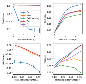
Simulation studies. We first study datasets that simulate the unfair admissions committee from Eq. 1. We fix the effect of test score on admissions to . We generate multiple datasets by varying the committee’s bias due to sex and the historical disadvantage on test score .
Fig. 4 show how eo-fairness and predictive accuracy trade off as the bias increases. Only the eo predictor and ftu achieve eo fairness. Although both are less accurate than classical ml, the eo predictor achieves greater accuracy than ftu. Fig. 4 show how aa-fairness and predictive accuracy trade off as the historical disadvantage increases. Only aa and FairLearning achieve aa-fairness. Among these aa-fair predictors, the aa predictor is more accurate.
Case studies. We study the fair algorithms on three real datasets: 1) Adult income for predicting whether individuals’ income is higher than $50K, 2) ProPublica’s COMPAS for predicting recidivism scores 3) German credit for predicting whether individuals have good or bad credit. For Adult and COMPAS, both gender and race are sensitive attributes. For German credit, gender and marital status are sensitive attributes. Decisions are binary except for real-valued COMPAS recidivism scores.
| Metrics () on Adult | ||||
| eo | aa | KL | Prediction | |
| 2.5 | 16.2 | 15.0 | 78.6 | |
| ftu | 0 | 14.8 | 12.2 | 77.3 |
| 0 | 14.1 | 12.6 | 77.4 | |
| FL | -14.8 | 0 | 5.3 | 75.1 |
| -9.1 | 0 | 1.5 | 77.1 | |
Fig. 4 reports results on the Adult dataset. (In Appendix D, we report results on the COMPAS and German credit datasets, and provide all the details needed to reproduce our studies.) The table reports accuracy, eo, and aa. Further, to measure demographic parity, it reports the KL divergence between decisions and ; when there is demographic parity, the KL is close to zero.
The findings are consistent with the simulation studies. The eo and ftu predictors achieve eo-fairness and, among these, the eo predictor is more accurate. The aa predictor and FairLearning achieve aa-fairness and demographic parity; but the aa predictor is more accurate because it uses all of the attributes. While the ml predictor has the best accuracy, it is less eo-fair and aa-fair.
5 Discussion
We develop fair ML algorithms that modify fitted ML predictors to make them fair. We prove that the resulting predictors are eo-fair or aa-fair, and that they otherwise maximally recover the fitted ML predictor. We show empirically that the eo and aa predictors produce better predictions than existing algorithms for satisfying the same fairness criteria.
The eo and aa predictors both aim to recover the ML outcome as much as possible. However, they can also readily extend to recover the ground truth outcome subject to availability of data. For example, instead of predicting the admissions decision accurately, we can aim the eo and aa predictors for the ground truth outcome, i.e. first year GPA. They will lead to fair and accurate predictions of whether the applicants’ succeed in college.
References
Appendix
Appendix A Proof of Theorem 1
Before proving the eo-fairness and optimality of the eo predictor, we first establish a lemma about eo-fairness. It says the eo-fairness of a decision is equivalent to no causal arrow from to .
Lemma 3.
(eo No ) Assume the causal graph in Fig. 2. A decision satisfies equal opportunities over if and only if there is no causal arrow between and .
Consider a decision in the causal graphical model Fig. 5(b). The reason behind Lemma 3 is that in Fig. 5(b) (pearl2009causality). So eo reduces to being constant in .
Lemma 3 shows that the decision is eo-fair as long as does not predict using the sensitive attribute.
Proof.
The goal is to show that counterfactual fairness is equivalent to
| (6) |
for any . This equation is equivalent to no causal arrow between and .
We start with the definition of eo-fairness.
| (7) | ||||
| (8) | ||||
| (9) |
Eq. 8 is due to the observation that . Eq. 9 is true because
| (10) |
for any . The last equation is equivalent to no causal arrow from to .
∎
Now we are ready to prove Theorem 1.
Proof.
As a direct application of Lemma 3, we prove the first part of Theorem 1: is eo-fair. The reason is that as is defined in Eq. 4.
We then prove the second part of Theorem 1. It establishes the optimality of .
We start with rewriting the goal of the proof. We will show this goal is equivalent to the definition of the eo predictor.
| (11) | ||||
| (12) | ||||
| (13) | ||||
| (14) | ||||
| (15) | ||||
| (16) | ||||
| (17) | ||||
| (18) | ||||
| (19) |
Eq. 11 is the goal of the proof. Eq. 12 is due to the definition of the Kullback-Leibler (kl) divergence. Eq. 13 is due to being a given random variable. LABEL:eq:step4 is due to Lemma 3. Eq. 15 switches the integral subject to conditions of the dominated convergence theorem. Eq. 16 is due to Fig. 5(b) and the backdoor adjustment formula of pearl2009causality. Eq. 17 is due to the definition of the kl divergence and being given. Eq. 18 is because setting has for all . The expecation is hence also zero: . Eq. 19 is due to the definition of the intervention distribution (pearl2009causality).
This calculation implies minimizes the average kl between the ML decision and the eo decision . the eo predictor maximally recovers the ML decision. Put differently, the eo predictor minimally modifies the ML decision to achieve eo-fairness.
∎
Appendix B Proof of Theorem 2
Proof.
We first prove that the aa predictor is aa-fair.
Recall the definition of the aa predictor:
| (20) |
Note the above equation is the same definition as in Eq. 5. We simply change to for downstream notation convenience.
This implies
| (21) |
Hence we have
| (22) | ||||
| (23) | ||||
| (24) |
Eq. 24 is due to by the structural equation implied by the causal graph:
| (25) |
The intuition here is the observed will provide the same information as for the same person. They all contain the information about the background variable that affects . We hence have .
Notice that the right hand side of Eq. 24 does not depend on . This implies . We simply repeat the same calculation for .
We hence have proved that the aa predictor is aa-fair:
| (26) |
It establishes the first part of Theorem 2.
We can also prove demographic parity for .
| (27) | ||||
| (28) | ||||
| (29) | ||||
| (30) |
The third equality is due to by Pearl’s twin network (pearl2009causality).
We next compute the marginal distribution of .
| (32) | ||||
| (33) | ||||
| (34) |
Therefore, we have
| (36) |
Hence,
| (37) |
This establishes demographic parity.
We next prove the second part of Theorem 2. We show that minimizes . In fact, recovers the marginal distribution of .
| (38) | ||||
| (39) | ||||
| (40) | ||||
| (41) | ||||
| (42) | ||||
| (43) |
This gives . Hence, minimizes this kl and preserves the marginal distribution of .
∎
Appendix C The correctness of Alg. 1
We leverage the backdoor adjustment formula in pearl2009causality to compute from the past admissions records .
Proposition 4.
Assume the causal graph Fig. 5(a). The eo predictor can be computed using the observed data :
| (44) |
if
| (45) |
for all , and
Proof.
Proposition 4 is a direct consequence of Theorem 3.3.2 of pearl2009causality. ∎
Eq. 44 reiterates the fact that does not simply ignore the sensitive attribute ; estimating relies on in the training data. However, does not rely on in the test data.
We leverage the abduction-action-prediction approach (pearl2009causality) to compute .
Proposition 5.
Assume the causal graph Fig. 5(a). Write
| (46) |
for some function and zero mean random variable satisfying . The aa predictor can be computed using the observed data :
| (47) | ||||
| (48) |
where .
Proof.
Alg. 1 can easily generalize to cases where sensitive attributes are unobserved. In these cases, we can leverage recent techniques in multiple causal inference like the approach from wang2018blessings. These approaches construct substitutes for the unobserved sensitive attributes from the descendants of the sensitive attributes.
Appendix D Detailed results of the empirical studies
We study the fair algorithms on three real datasets:
-
•
Adult income dataset.444https://www.kaggle.com/wenruliu/adult-income-dataset The task is to predict whether someone has a yearly income higher than $50K; the decision is binary. The sensitive attributes are gender and race; other attributes include education and marital status. The dataset has 32,561 training samples and 16,282 test samples.
-
•
ProPublica’s COMPAS recidivism data. The task is to predict an individual’s recidivism score; the decision is real-valued. The sensitive attributes are gender and race; other attributes include the priors count, juvenile felonies count, and juvenile misdemeanor count. The dataset has 6,907 complete samples. We split them into 75% training and 25% testing.
-
•
German credit data.555https://www.kaggle.com/uciml/german-credit The task is to predict whether an individual has good or bad credit; the decision is binary. The sensitive attributes are gender and marital status; other attributes include credit history, savings, and employment history. The dataset has 1,000 samples. We split them into 75% training and 25% testing.
We report the detailed results of the COMPAS dataset and the German credit dataset in Appendix D and Appendix D.
| Metrics () on COMPAS | |||||
| eo | aa | KL | Prediction | ||
| ML predictor | -68.1 | -104.9 | 17.1 | 28.0 | |
| \cdashline1-5 ftu | 0 | -52.9 | 0.5 | 25.6 | |
| eo predictor | 0 | -36.8 | 0.5 | 25.6 | |
| \cdashline1-5 FairLearning | -41.2 | 0 | 0.2 | 22.7 | |
| aa predictor | -41.2 | 0 | 0.2 | 22.7 | |
| Metrics () on German Credit | |||||
| eo | aa | kl | Prediction | ||
| ML predictor | -5.4 | -3.9 | 18.6 | 64.7 | |
| \cdashline1-5 ftu | 0 | -2.0 | 15.6 | 63.4 | |
| eo predictor | 0 | 1.5 | 13.2 | 64.5 | |
| \cdashline1-5 FairLearning | -1.4 | 0 | 8.3 | 63.5 | |
| aa predictor | -1.3 | 0 | 7.8 | 64.3 | |
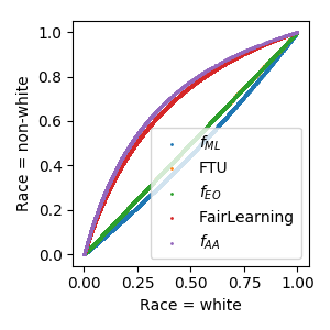
We further discuss eo-fairness and aa-fairness. Consider the eo-fairness against race. For the Adult dataset, Fig. 6(a) plots against , where and only differ by the individual’s race being white or non-white. A method is eo-fair if the predictions align with the diagonal. Both the eo predictor and ftu align with the diagonal; they are eo-fair. None of classical ML, FairLearning, or the aa predictor are eo-fair, and counterfactual aa and FairLearning are less eo-fair than classical ML.
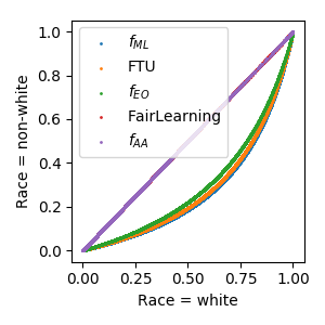
Now consider the aa-fairness against race. For the Adult dataset, Fig. 6(b) plots against when and differ by whether the individual is white or non-white. If the predictions align with the diagonal, the decision is aa-fair. Both the aa predictor and FairLearning align with the diagonal; they are counterfactually fair. Counterfactual eo is less unfair than ftu. The classical ML predictor is most unfair. (These results generalize across datasets.)
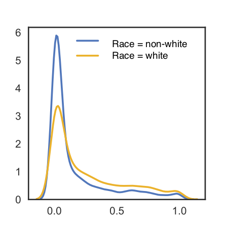
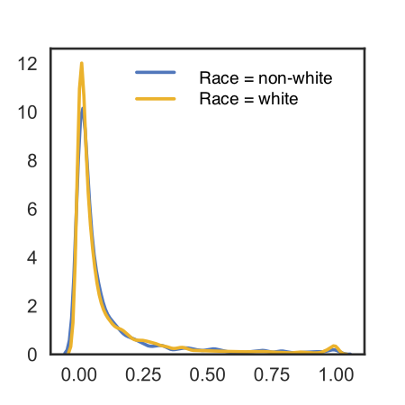
Finally, we discuss demographic parity. Demographic parity is a group-level statistical measure that requires decisions to be independent of sensitive attributes. It has been used to measure affirmative action (dwork2012fairness). To evaluate demographic parity, we compare the prediction distributions between the groups of individuals with different sensitive attributes. The metric is the symmetric kl divergence between and . For a predictor achieving demographic parity, the kl is zero. (We evaluate the symmetric kl by binning the values of predictions.)
Fig. 4 present the symmetric kl between the two gender groups in the data. Both the aa predictor and FairLearning have close-to-zero symmetric kl. The aa predictor generally has lower symmetric kl; it is closer to demographic parity. None of the other methods are close.
Now consider the demographic parity against race. Fig. 7 demonstrates the prediction distributions of white and non-white individuals. While classical ML has very different prediction distributions for the two groups, the prediction distributions of the aa predictor is nearly identical.