Asymptotic learning curves of kernel methods: empirical data v.s. Teacher-Student paradigm

Stefano Spigler Institute of Physics, École Polytechnique Fédérale de Lausanne, 1015 Lausanne, Switzerland Mario Geiger Institute of Physics, École Polytechnique Fédérale de Lausanne, 1015 Lausanne, Switzerland Matthieu Wyart Institute of Physics, École Polytechnique Fédérale de Lausanne, 1015 Lausanne, Switzerland
Abstract

How many training data are needed to learn a supervised task? It is often observed that the generalization error decreases as nβsuperscript𝑛𝛽n^{-\beta} where n𝑛n is the number of training examples and β𝛽\beta an exponent that depends on both data and algorithm. In this work we measure β𝛽\beta when applying kernel methods to real datasets. For MNIST we find β0.4𝛽0.4\beta\approx 0.4 and for CIFAR10 β0.1𝛽0.1\beta\approx 0.1, for both regression and classification tasks, and for Gaussian or Laplace kernels. To rationalize the existence of non-trivial exponents that can be independent of the specific kernel used, we study the Teacher-Student framework for kernels. In this scheme, a Teacher generates data according to a Gaussian random field, and a Student learns them via kernel regression. With a simplifying assumption — namely that the data are sampled from a regular lattice — we derive analytically β𝛽\beta for translation invariant kernels, using previous results from the kriging literature. Provided that the Student is not too sensitive to high frequencies, β𝛽\beta depends only on the smoothness and dimension of the training data. We confirm numerically that these predictions hold when the training points are sampled at random on a hypersphere. Overall, the test error is found to be controlled by the magnitude of the projection of the true function on the kernel eigenvectors whose rank is larger than n𝑛n. Using this idea we predict the exponent β𝛽\beta from real data by performing kernel PCA, leading to β0.36𝛽0.36\beta\approx 0.36 for MNIST and β0.07𝛽0.07\beta\approx 0.07 for CIFAR10, in good agreement with observations. We argue that these rather large exponents are possible due to the small effective dimension of the data.

1 Introduction

In supervised learning machines learn from a finite collection of n𝑛n training data, and their generalization error is then evaluated on unseen data drawn from the same distribution. How many data are needed to learn a task is characterized by the learning curve relating generalization error to n𝑛n. In various cases, the generalization error decays as a power law nβsuperscript𝑛𝛽n^{-\beta}, with an exponent β𝛽\beta that depends on both the data and the algorithm. In [1] β𝛽\beta is reported for state-of-the-art (SOTA) deep neural networks for various tasks: in for neural-machine translation β0.3𝛽0.3\beta\approx 0.30.360.360.36 (for fixed model size) or β0.13𝛽0.13\beta\approx 0.13 (for best-fit models at any n𝑛n); language modeling shows β0.06𝛽0.06\beta\approx 0.060.090.090.09; in speech recognition β0.3𝛽0.3\beta\approx 0.3; SOTA models for image classification (on ImageNet) have exponents β0.3𝛽0.3\beta\approx 0.30.50.50.5. Currently there is no available theory of deep learning to rationalize these observations. Recently it was shown that for a proper initialization of the weights, deep learning in the infinite-width limit [2] converges to kernel learning. Moreover, it is nowadays part of the lore that there exist kernels whose performance is nearly comparable to deep networks [3, 4], at least for some tasks. It is thus of great interest to understand the learning curves of kernels. For regression, if the target function being learned is simply assumed to be Lipschitz, then the best guarantee is β=1/d𝛽1𝑑\beta=\nicefrac{{1}}{{d}} [5, 6] where d𝑑d is the data dimension. Thus for large d𝑑d, β𝛽\beta is very small: learning is completely inefficient, a phenomenon referred to as the curse of dimensionality. As a result, various works on kernel regression make the much stronger assumption that the training points are sampled from a target function that belongs to the reproducing kernel Hilbert space (RKHS) of the kernel (for Gaussian r [7]). With this assumption β𝛽\beta does not depend on d𝑑d (for instance in  [8] β=1/2𝛽12\beta=1/2 is guaranteed). Yet, RKHS is a very strong assumption which requires the smoothness of the target function to increase with d𝑑d [6] (for Gaussian random fields see Appendix H), which may not be realistic in large dimensions.

In Section 3 we compute β𝛽\beta empirically for kernel methods applied on MNIST and CIFAR10 datasets. We find βMNIST0.4subscript𝛽MNIST0.4\beta_{\mathrm{MNIST}}\approx 0.4 and βCIFAR100.1subscript𝛽CIFAR100.1\beta_{\mathrm{CIFAR10}}\approx 0.1 respectively. Quite remarkably, we observe essentially the same exponents for regression and classification tasks, using either a Gaussian or a Laplace kernel. Thus the exponents are not as small as 1/d1𝑑\nicefrac{{1}}{{d}} (d=784𝑑784d=784 for MNIST, d=3072𝑑3072d=3072 for CIFAR10), but neither are they 1/212\nicefrac{{1}}{{2}} as one would expect under the RKHS assumption. These facts call for frameworks in which assumptions on the smoothness of the data can be intermediary between Lipschitz and RKHS. Here we study such a framework for regression, in which the target function is assumed to be a Gaussian random field of zero mean with translation-invariant isotropic covariance KT(x¯)subscript𝐾𝑇¯𝑥K_{T}(\underline{x}). The data can equivalently be thought as being synthesized by a “Teacher” kernel KT(x¯)subscript𝐾𝑇¯𝑥K_{T}(\underline{x}). Learning is performed with a “Student” kernel KS(x¯)subscript𝐾𝑆¯𝑥K_{S}(\underline{x}) that minimizes the mean-square error. In general KT(x¯)KS(x¯)subscript𝐾𝑇¯𝑥subscript𝐾𝑆¯𝑥K_{T}(\underline{x})\neq K_{S}(\underline{x}). In this set-up learning is very similar to a technique referred to as kriging, or Gaussian process regression, originally developed in the geostatistics community [9, 10].

To quantify learning, in Section 4 we first perform numerical experiments for data points distributed uniformly at random on a hypersphere of varying dimension d𝑑d, focusing on a Laplace kernel for the Student, and considering a Laplace or Gaussian kernel for the Teacher. We observe that in both cases β(d)𝛽𝑑\beta(d) is a decreasing function. In Section 5, to derive β(d)𝛽𝑑\beta(d) we consider the simplified situation where the Gaussian random field is sampled at training points lying on a regular lattice. Building on the kriging literature  [10], we show that β𝛽\beta is controlled by the high-frequency scaling of both the Teacher and Student kernels: assuming that the Fourier transforms of the kernels decay as K~T(w¯)=cTw¯αT+o(w¯αT)subscript~𝐾𝑇¯𝑤subscript𝑐𝑇superscriptnorm¯𝑤subscript𝛼𝑇𝑜superscriptnorm¯𝑤subscript𝛼𝑇\tilde{K}_{T}(\underline{w})=c_{T}|\!|\underline{w}|\!|^{-\alpha_{T}}+o\left(|\!|\underline{w}|\!|^{-\alpha_{T}}\right) and K~S(w¯)=cSw¯αS+o(w¯αS)subscript~𝐾𝑆¯𝑤subscript𝑐𝑆superscriptnorm¯𝑤subscript𝛼𝑆𝑜superscriptnorm¯𝑤subscript𝛼𝑆\tilde{K}_{S}(\underline{w})=c_{S}|\!|\underline{w}|\!|^{-\alpha_{S}}+o\left(|\!|\underline{w}|\!|^{-\alpha_{S}}\right), we obtain

β=1dmin(αTd,2αS).𝛽1𝑑subscript𝛼𝑇𝑑2subscript𝛼𝑆\beta=\frac{1}{d}\min(\alpha_{T}-d,2\alpha_{S}). (1)

Importantly (i) Eq. (1) leads to a prediction for β(d)𝛽𝑑\beta(d) that accurately matches our numerical study for random training data points, leading to the conjecture that Eq. (1) holds in that case as well. We offer the following interpretation: ultimately, kernel methods are performing a local interpolation whose quality depends on the distance δ(n)𝛿𝑛\delta(n) between adjacent data points. δ(n)𝛿𝑛\delta(n) is asymptotically similar for random data or data sitting on a lattice. (ii) If the kernel KSsubscript𝐾𝑆K_{S} is not too sensitive to high-frequencies, then learning is optimal as far as scaling is concerned and β=(αTd)/d𝛽subscript𝛼𝑇𝑑𝑑\beta=(\alpha_{T}-d)/d. We will argue that the smoothness index s[(αTd)/2]𝑠delimited-[]subscript𝛼𝑇𝑑2s\equiv[(\alpha_{T}-d)/2] characterizes the number of derivatives of the target function that are continuous. We thus recover the curse of dimensionality: s𝑠s needs to be of order d𝑑d to have non-vanishing β𝛽\beta in large dimensions.

We show that in some regime, the test error for Gaussian data is controlled by an exponent a𝑎a describing how the coefficients of the true function in the eigenbasis of the kernel decay with rank. We estimate a𝑎a by the kernel principal component analysis (kernel PCA) based on diagonalizing the Gram matrix. This measure yields a prediction for the learning curve exponent β𝛽\beta that matches the numerical fit, with βMNIST0.36subscript𝛽MNIST0.36\beta_{\mathrm{MNIST}}\approx 0.36 and βCIFAR100.07subscript𝛽CIFAR100.07\beta_{\mathrm{CIFAR10}}\approx 0.07. We show in Appendix I using the recent formalism of [11], which does not assume Gaussianity but makes more technical assumptions, that the result of our theorem Eq.1 is recovered, supporting further its validity for real data.

Finally, we discuss the following apparent paradox: β𝛽\beta is significant for MNIST and CIFAR10, for which d𝑑d is a priori very large, leading to a smoothness value s𝑠s in the hundreds in both cases, which appears unrealistic. In Section 7 The paradox is resolved by considering that real datasets actually live on lower-dimensional manifolds. As far as kernel learning is concerned, our findings support that the correct definition of dimension should be based on how the nearest-neighbors distance δ(n)𝛿𝑛\delta(n) scales with n𝑛n: δ(n)n1/deffsimilar-to𝛿𝑛superscript𝑛1subscript𝑑eff\delta(n)\sim n^{-\nicefrac{{1}}{{d_{\mathrm{eff}}}}}. Direct measurements of δ(n)𝛿𝑛\delta(n) support that MNIST and CIFAR10 live on manifolds of lower dimensions dMNISTeff15subscriptsuperscript𝑑effMNIST15d^{\mathrm{eff}}_{\mathrm{MNIST}}\approx 15 and dCIFAR10eff35subscriptsuperscript𝑑effCIFAR1035d^{\mathrm{eff}}_{\mathrm{CIFAR10}}\approx 35.

2 Related works

Part of the literature has investigated the problem of kernel regression from a different point of view, namely the optimal worst-case performance (see for instance [12, 13, 14]). The target function is not assumed to be generated by a Gaussian random field, but its regularity is controlled using a source condition that constrains the decay of its coefficients in the eigenbasis of the kernel. For uniform data distributions and isotropic kernels this is similar to controlling how the Fourier transform of the target function decays at high frequency. What we study in the present work is, on the contrary, the typical performance. Indeed, it turns out that both the worst-case and the typical learning curve decay as power laws, and the latter decays faster.

The Teacher-Student framework for kernel regression was previously introduced in [15, 16], where a formula for the learning curve was derived based on a few uncontrolled approximations. It is easy to show that their results match the predictions of our theorem, although in [16] the case where the performance is limited by the Student (αTd>2αSsubscript𝛼𝑇𝑑2subscript𝛼𝑆\alpha_{T}-d>2\alpha_{S}) is ignored. More recently, [11] generalized this approach using similar approximations and extended it to kernel regression applied to any target function (or ensemble thereof). Kernel PCA on MNIST was used to support that these approximations hold well on real data. An asymptotic scaling relation between β𝛽\beta and a𝑎a was obtained, again the presence of other regimes was not noted. By contrast we perform an exact calculations for the asymptotic behavior of Gaussian data on a lattice. In Appendix I we show that the two approaches are consistent and lead to the same asymptotic predictions for β𝛽\beta.

Our set-up of Teacher-Student learning with kernels is also referred to as kriging, or Gaussian process regression, and it was originally developed in the geostatistics community [9]. In Section 5 we present our theorem, that allows one to know the rate at which the test error decreases as we increase the number of training points, assumed to lie on a high-dimensional regular lattice. Similar results have been previously derived in the kriging literature [10] when sampling occurs on the regular lattice with the exception of the origin, where the inference is made. Here we propose an alternative derivation that some readers might find simpler. We also study a slightly different problem: instead of computing the test error when the inference is carried on at the origin, we compute the average error for a test point that lie at an arbitrary point, sampled uniformly at random and not necessarily on the lattice. Then, in what follows we show, via extensive numerical simulations, that such predictions are accurate even when the training points do not lie on a regular lattice, but are taken at random on a hypersphere. An exact proof of our result in such a general setting is difficult and cannot be found even in the kriging literature. To our knowledge the results that get closer to the point are those discussed in [17], where the author studies one-dimensional processes where the training data are not necessarily evenly spaced.

In this work the effective dimension of the data plays an import role, as it controls how the distance between nearest neighbors scales with the dataset size. Of course, there exists a vast literature  [18, 19, 20, 21, 22, 23, 24] devoted to the study of effective dimensions, where other definitions are analyzed. The effective dimensions that we find are compatible with those obtained with more refined methods.

3 Learning curve for kernel methods applied to real data

In what follows we apply kernel methods to the MNIST and CIFAR10 datasets, each consisting of a set of images (x¯μ)μ=1nsuperscriptsubscriptsubscript¯𝑥𝜇𝜇1𝑛(\underline{x}_{\mu})_{\mu=1}^{n}. We simplify the problem by considering only two classes whose label Z(x¯μ)=±1𝑍subscript¯𝑥𝜇plus-or-minus1Z(\underline{x}_{\mu})=\pm 1 correspond to odd and even numbers for MNIST, and to two groups of 5 classes in CIFAR10. The goal is to infer the value of the label Z^S(x¯)subscript^𝑍𝑆¯𝑥\hat{Z}_{S}(\underline{x}) of an image x¯¯𝑥\underline{x} that does not belong to the dataset. The S𝑆S subscript reminds us that inference is performed using a positive definite kernel KSsubscript𝐾𝑆K_{S}. We perform inference in both a regression and a classification setting. The following algorithms and associated results can be found in [25].

Regression.

Learning corresponds to minimizing a mean-square error:

minμ=1n[Z^S(x¯μ)Z(x¯μ)]2.superscriptsubscript𝜇1𝑛superscriptdelimited-[]subscript^𝑍𝑆subscript¯𝑥𝜇𝑍subscript¯𝑥𝜇2\min\sum_{\mu=1}^{n}\left[\hat{Z}_{S}(\underline{x}_{\mu})-Z(\underline{x}_{\mu})\right]^{2}. (2)

For algorithms seeking solutions of the form Z^S(x¯)=μaμKS(x¯μ,x¯)a¯k¯S(x¯)subscript^𝑍𝑆¯𝑥subscript𝜇subscript𝑎𝜇subscript𝐾𝑆subscript¯𝑥𝜇¯𝑥¯𝑎subscript¯𝑘𝑆¯𝑥\hat{Z}_{S}(\underline{x})=\sum_{\mu}a_{\mu}K_{S}(\underline{x}_{\mu},\underline{x})\equiv\underline{a}\cdot\underline{k}_{S}(\underline{x}) by minimizing the man-square loss over the vector a¯¯𝑎\underline{a}, one obtains:

Z^S(x¯)=k¯S(x¯)𝕂S1Z¯,subscript^𝑍𝑆¯𝑥subscript¯𝑘𝑆¯𝑥superscriptsubscript𝕂𝑆1¯𝑍\hat{Z}_{S}(\underline{x})=\underline{k}_{S}(\underline{x})\cdot\mathbb{K}_{S}^{-1}\underline{Z}, (3)

where the vector Z¯¯𝑍\underline{Z} contains all the labels in the training set, Z¯(Z(x¯μ))μ=1n¯𝑍superscriptsubscript𝑍subscript¯𝑥𝜇𝜇1𝑛\underline{Z}\equiv(Z(\underline{x}_{\mu}))_{\mu=1}^{n}, and 𝕂S,μνKS(x¯μ,x¯ν)subscript𝕂𝑆𝜇𝜈subscript𝐾𝑆subscript¯𝑥𝜇subscript¯𝑥𝜈\mathbb{K}_{S,\mu\nu}\equiv K_{S}(\underline{x}_{\mu},\underline{x}_{\nu}) is the Gram matrix. The Gram matrix is always invertible if the kernel KSsubscript𝐾𝑆K_{S} is positive definite. The generalization error is then evaluated as the expected mean-square error on unseen data, estimated by averaging over a test set composed of ntestsubscript𝑛testn_{\mathrm{test}} unseen data points:

MSE=1ntestμ=1ntest[Z^S(x¯μ)Z(x¯μ)]2.MSE1subscript𝑛testsuperscriptsubscript𝜇1subscript𝑛testsuperscriptdelimited-[]subscript^𝑍𝑆subscript¯𝑥𝜇𝑍subscript¯𝑥𝜇2\mathrm{MSE}=\frac{1}{n_{\mathrm{test}}}\sum_{\mu=1}^{n_{\mathrm{test}}}\left[\hat{Z}_{S}(\underline{x}_{\mu})-Z(\underline{x}_{\mu})\right]^{2}. (4)

Classification.

We perform kernel classification via the algorithm soft-margin SVM. The details can be found in Appendix A. After learning from the training data with a student kernel KSsubscript𝐾𝑆K_{S}, performance is evaluated via the generalization error. It is estimated as the fraction of correctly predicted labels for data points belonging to a test set with ntestsubscript𝑛testn_{\mathrm{test}} elements.

Refer to caption
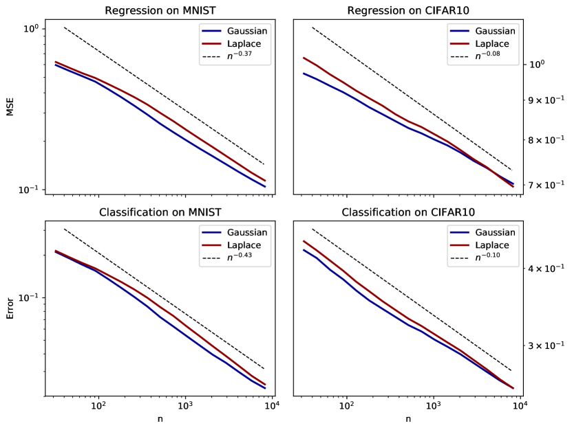
Figure 1: Learning curves for regression on MNIST and CIFAR10 (top row); and for classification on MNIST and CIFAR10 (bottom row). Curves are averaged over 400400400 runs. A power law is plotted to estimate the asymptotic behavior at large n𝑛n: the exponent is fitted on the last decade on the average of the two curves, since it does not seem to depend significantly on the specific kernel or on the task. In each setting we use both a Gaussian kernel K(x¯)exp(x¯2/(2σ2))proportional-to𝐾¯𝑥superscriptnorm¯𝑥22superscript𝜎2K(\underline{x})\propto\exp(-|\!|\underline{x}|\!|^{2}/(2\sigma^{2})) and a Laplace one K(x¯)exp(x¯/σ)proportional-to𝐾¯𝑥norm¯𝑥𝜎K(\underline{x})\propto\exp(-|\!|\underline{x}|\!|/\sigma), with σ=1000𝜎1000\sigma=1000.

In Fig. 1 we present the learning curves for (binary) MNIST and CIFAR10, for regression and classification. Learning is performed both with a Gaussian kernel K(x¯)exp(x¯2/(2σ2))proportional-to𝐾¯𝑥superscriptnorm¯𝑥22superscript𝜎2K(\underline{x})\propto\exp(-|\!|\underline{x}|\!|^{2}/(2\sigma^{2})) and a Laplace one K(x¯)exp(x¯/σ)proportional-to𝐾¯𝑥norm¯𝑥𝜎K(\underline{x})\propto\exp(-|\!|\underline{x}|\!|/\sigma). Remarkably, the power laws in the two tasks are essentially identical (although the estimated exponent appears to be slightly larger, in absolute value, for classification). Moreover, the two kernels display a very similar behavior, compatible with the same exponent: about 0.40.4-0.4 for MNIST and 0.10.1-0.1 for CIFAR10. The presented data are for σ=1000𝜎1000\sigma=1000; in Appendix B we show that the same behaviour is observed for different values.

4 Generalization scaling in kernel Teacher-Student problems

We study β𝛽\beta in a simplified setting where the data is assumed to follow a Gaussian distribution with known covariance. It falls into the class of teacher-Student problems, which are characterized by a machine (the Teacher) that generates the data, and another machine (the Student) that tries to learn from them. The Teacher-Student paradigm has been broadly used to study supervised learning  [26, 27, 15, 16, 28, 29, 30, 31, 32, 33]. He we restrict our attention to kernel methods: we assume that a target function is distributed according to a Gaussian random field Z𝒩(0,KT)similar-to𝑍𝒩0subscript𝐾𝑇Z\sim\mathcal{N}(0,K_{T}) — the Teacher — characterized by a translation-invariant isotropic covariance function KT(x¯,x¯)=KT(x¯x¯)subscript𝐾𝑇¯𝑥superscript¯𝑥subscript𝐾𝑇norm¯𝑥superscript¯𝑥K_{T}(\underline{x},\underline{x}^{\prime})=K_{T}(|\!|\underline{x}-\underline{x}^{\prime}|\!|), and that the training dataset consists the finite set of n𝑛n observations Z¯=(Z(x¯μ))μ=1n¯𝑍superscriptsubscript𝑍subscript¯𝑥𝜇𝜇1𝑛\underline{Z}=(Z(\underline{x}_{\mu}))_{\mu=1}^{n}. This is equivalent to saying that the vector of training points follows a centered Gaussian distribution with a covariance matrix that depends on KTsubscript𝐾𝑇K_{T} and on the location of the points (x¯μ)μ=1nsuperscriptsubscriptsubscript¯𝑥𝜇𝜇1𝑛(\underline{x}_{\mu})_{\mu=1}^{n}:

Z¯𝒩(0¯,𝕂T),where𝕂T=(KT(x¯μ,x¯ν))μ,ν=1n.formulae-sequencesimilar-to¯𝑍𝒩¯0subscript𝕂𝑇wheresubscript𝕂𝑇superscriptsubscriptsubscript𝐾𝑇subscript¯𝑥𝜇subscript¯𝑥𝜈𝜇𝜈1𝑛\underline{Z}\sim\mathcal{N}\left(\underline{0},\mathbb{K}_{T}\right),\quad\mathrm{where}\quad\mathbb{K}_{T}=(K_{T}(\underline{x}_{\mu},\underline{x}_{\nu}))_{\mu,\nu=1}^{n}. (5)

Once the Teacher has generated the dataset, the rest follows as in the kernel regression described in the previous section. We use another translation-invariant isotropic kernel KS(x¯,x¯)subscript𝐾𝑆¯𝑥superscript¯𝑥K_{S}(\underline{x},\underline{x}^{\prime}) — the Student — to infer the value of the field at another point, Z^S(x¯)subscript^𝑍𝑆¯𝑥\hat{Z}_{S}(\underline{x}), with a regression task, i.e. minimizing the mean-square error in Eq. (2). The solution is therefore given again by Eq. (3).

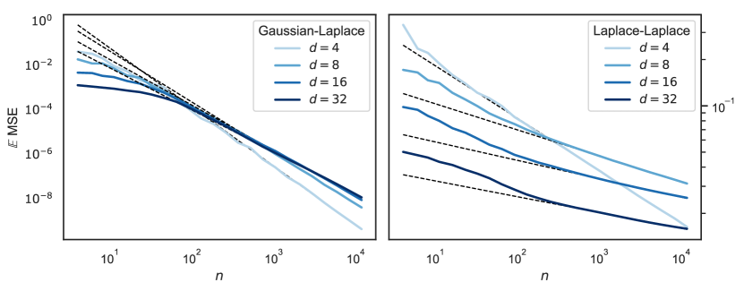
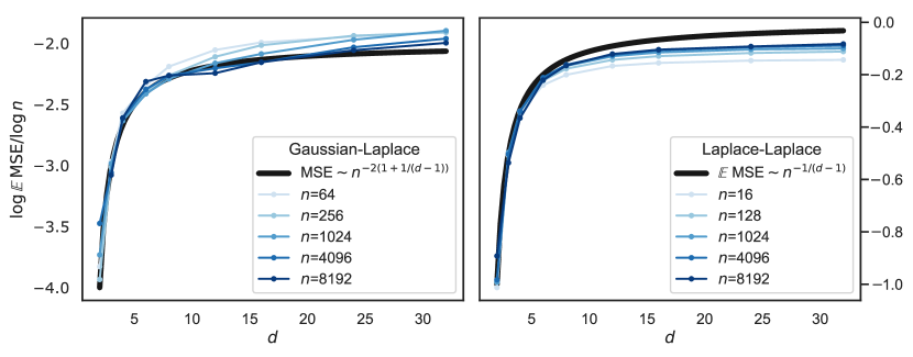
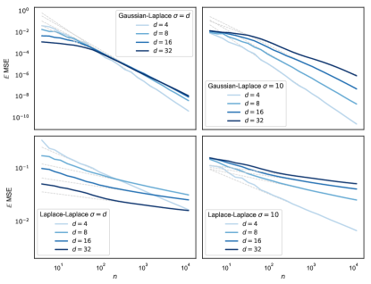
Fig. 2 (a-b) shows the mean-square error obtained numerically. In the examples the Student is always taken to be a Laplace kernel, and the Teacher is either a Laplace kernel or a Gaussian kernel. The points (x¯μ)μ=1nsuperscriptsubscriptsubscript¯𝑥𝜇𝜇1𝑛(\underline{x}_{\mu})_{\mu=1}^{n} are taken uniformly at random on the unit d𝑑d-dimensional hypersphere for several dimensions d𝑑d and for several dataset sizes n𝑛n. We take σS=σT=dsubscript𝜎𝑆subscript𝜎𝑇𝑑\sigma_{S}=\sigma_{T}=d as we observed that with this choice smaller datasets were enough to approach a limiting curve — in Appendix C we show the plots for the case σS=σT=10subscript𝜎𝑆subscript𝜎𝑇10\sigma_{S}=\sigma_{T}=10, which appears to converge to the same limit curve with increasing n𝑛n, but at a smaller pace. The figure shows that when n𝑛n is large enough, the mean-square error behaves as a power law (dashed lines) with an exponent that depends on the spatial dimension of the data, as well as on the kernels. The fitted exponents are plotted in Fig. 2 (c-d) as a function of the spatial dimension d𝑑d for different dataset sizes n𝑛n. In the next section we will discuss the theoretical prediction, that in the figure is plotted a thick black line. The figure shows that as the dataset gets bigger, the asymptotic exponent tends to our prediction. In Appendix D we present the learning curves of Gaussian Students with both a Laplace and a Gaussian kernel. When both kernels are Gaussian the test error decays exponentially fast, a result that matches our theoretical prediction. In Appendix E we also provide further numerical results for the case where the Teacher kernel is a Matérn kernel (as defined therein).
Refer to caption
Refer to caption
Figure 2: Results for the Teacher-Student kernel regression problem, where the Student is always a Laplace kernel. Data points are sampled uniformly at random on a d𝑑d-dimensional hypersphere. (Top row) Mean-square error versus the size of the training dataset, for Gaussian and Laplace Teachers and for multiple spatial dimensions. Dotted lines are the fitted power laws — we fit starting from n=700𝑛700n=700. (Bottom row) Fitted exponent β=log𝔼MSE/logn𝛽𝔼MSE𝑛-\beta=\log\mathbb{E}\,\mathrm{MSE}/\log n against the spatial dimension, for several dataset sizes. We fit from n=0𝑛0n=0 to a varying n𝑛n (written in the legends). The thick black lines are the theoretical predictions.

5 Analytic asymptotics for the kernel Teacher-Student problem on a lattice

In this section we compute analytically the exponent that describe the asymptotic decay of the generalization error when the number n𝑛n of training data increases. In order to derive the result we assume that both the Teacher Gaussian random field lives on a bounded hypercube, x¯𝒱[0,L]d¯𝑥𝒱superscript0𝐿𝑑\underline{x}\in\mathcal{V}\equiv[0,L]^{d}, where L𝐿L is a constant and d𝑑d is the spatial dimension. The fields and the kernels can then be thought of as L𝐿L-periodic along each dimension. Furthermore, to make the problem tractable we assume that the points (x¯μ)μ=1nsuperscriptsubscriptsubscript¯𝑥𝜇𝜇1𝑛(\underline{x}_{\mu})_{\mu=1}^{n} live on a regular lattice, covering all the hypercube 𝒱𝒱\mathcal{V}. Therefore, the linear spacing between neighboring points is δ=Ln1/d𝛿𝐿superscript𝑛1𝑑\delta=Ln^{-\nicefrac{{1}}{{d}}}. This is a different setting than the one used in the numerical simulations presented in the previous section for which the data distribution if Gaussian, showing that our results below are robust to such differences.

Generalization error is then evaluated via the typical mean-square error

𝔼MSE=𝔼[Z(x¯)Z^S(x¯)]2,𝔼MSE𝔼superscriptdelimited-[]𝑍¯𝑥subscript^𝑍𝑆¯𝑥2\mathbb{E}\,\mathrm{MSE}=\mathbb{E}\left[Z(\underline{x})-\hat{Z}_{S}(\underline{x})\right]^{2}, (6)

where the expectation is taken over both the Teacher process and the point x¯¯𝑥\underline{x} at which we estimate the field, assumed to be uniformly distributed in the hypercube 𝒱𝒱\mathcal{V}. In Appendix F we prove the following:

{theorem}

Let K~T(w¯)=cTw¯αT+o(w¯αT)subscript~𝐾𝑇¯𝑤subscript𝑐𝑇superscriptnorm¯𝑤subscript𝛼𝑇𝑜superscriptnorm¯𝑤subscript𝛼𝑇\tilde{K}_{T}(\underline{w})=c_{T}|\!|\underline{w}|\!|^{-\alpha_{T}}+o\left(|\!|\underline{w}|\!|^{-\alpha_{T}}\right) and K~S(w¯)=cSw¯αS+o(w¯αS)subscript~𝐾𝑆¯𝑤subscript𝑐𝑆superscriptnorm¯𝑤subscript𝛼𝑆𝑜superscriptnorm¯𝑤subscript𝛼𝑆\tilde{K}_{S}(\underline{w})=c_{S}|\!|\underline{w}|\!|^{-\alpha_{S}}+o\left(|\!|\underline{w}|\!|^{-\alpha_{S}}\right) as w¯norm¯𝑤|\!|\underline{w}|\!|\to\infty, where K~T(w¯)subscript~𝐾𝑇¯𝑤\tilde{K}_{T}(\underline{w}) and K~S(w¯)subscript~𝐾𝑆¯𝑤\tilde{K}_{S}(\underline{w}) are the Fourier transforms of the kernels KT(x¯)subscript𝐾𝑇¯𝑥K_{T}(\underline{x}), KS(x¯)subscript𝐾𝑆¯𝑥K_{S}(\underline{x}) respectively, assumed to be positive definite. We assume that K~T(w¯)subscript~𝐾𝑇¯𝑤\tilde{K}_{T}(\underline{w}) and K~S(w¯)subscript~𝐾𝑆¯𝑤\tilde{K}_{S}(\underline{w}) have a finite limit as w¯0norm¯𝑤0|\!|\underline{w}|\!|\to 0 and that K(0¯)<𝐾¯0K(\underline{0})<\infty. Then,

𝔼MSE=nβ+o(nβ)withβ=1dmin(αTd,2αS).formulae-sequence𝔼MSEsuperscript𝑛𝛽𝑜superscript𝑛𝛽with𝛽1𝑑subscript𝛼𝑇𝑑2subscript𝛼𝑆\mathbb{E}\,\mathrm{MSE}=n^{-\beta}+o\left(n^{-\beta}\right)\quad\mathrm{with}\quad\beta=\frac{1}{d}\min(\alpha_{T}-d,2\alpha_{S}). (7)

Moreover, in the case of a Gaussian kernel the result holds valid if we take the corresponding exponent to be α=𝛼\alpha=\infty.

Apart from the specific value of the exponent in Eq. (7), Theorem 5 implies that if the Student kernel decays fast enough in the frequency domain, then β𝛽\beta depends only on the data through the behaviour of the Teacher kernel at high frequencies. One then recovers β=(αTd)/d𝛽subscript𝛼𝑇𝑑𝑑\beta=(\alpha_{T}-d)/d, also found for the Bayes-optimal setting where the Student is identical to the Teacher.

Consider the predictions of Theorem 5 in the cases presented in Fig. 2 (a-b) of Gaussian and Laplace kernels. If both kernels are Laplace kernels then αT=αS=d+1subscript𝛼𝑇subscript𝛼𝑆𝑑1\alpha_{T}=\alpha_{S}=d+1 and 𝔼MSEn1/dsimilar-to𝔼MSEsuperscript𝑛1𝑑\mathbb{E}\,\mathrm{MSE}\sim n^{-\nicefrac{{1}}{{d}}}, which scales very slowly with the dataset size in large dimensions. If the Teacher is a Gaussian kernel (αT=subscript𝛼𝑇\alpha_{T}=\infty) and the Student is a Laplace kernel then β=2(1+1/d)𝛽211𝑑\beta=2(1+1/d), leading to β2𝛽2\beta\rightarrow 2 as d𝑑d\rightarrow\infty. In Fig. 2 (c-d) we compare these predictions with the exponents extracted from Fig. 2 (a-b). We plot log𝔼MSE/lognβ𝔼MSE𝑛𝛽\log\mathbb{E}\,\mathrm{MSE}/\log n\equiv-\beta, against the dimension d𝑑d of the data, varying the dataset size n𝑛n. The exponents extracted numerically tend to our analytical predictions when n𝑛n is large enough.

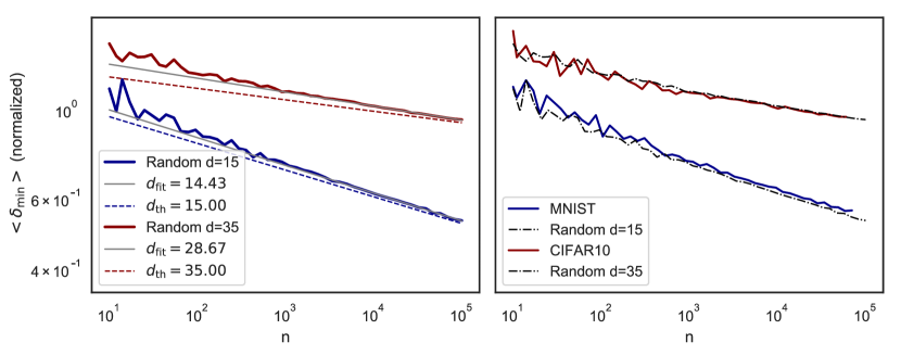
Notice that, although the theory and the experiments do not assume the same distribution for the sampling points (x¯μ)μ=1nsuperscriptsubscriptsubscript¯𝑥𝜇𝜇1𝑛(\underline{x}_{\mu})_{\mu=1}^{n}, this does not seem to yield any difference in the asymptotic behavior of the generalization error, leading to the conjecture that our predictions are exact even when the training set is random, and does not correspond to a lattice. The conjecture can be proven in one dimension following results of the kriging literature  [17], but generalization to higher d𝑑d is a much harder problem. Intuitively, for kernel learning performs an expansion, whose quality is governed by the target function smoothness and the typical distance δminsubscript𝛿\delta_{\min{}} between a point and its nearest neighbors in the training set. Both for random points or on a lattice, one has δminn1/dsimilar-tosubscript𝛿superscript𝑛1𝑑\delta_{\min{}}\sim n^{-\nicefrac{{1}}{{d}}} when n𝑛n is large enough, thus both situations lead to the same β𝛽\beta. This is shown in Fig. 4 (left).

Theorem 5 underlines that kernel methods are subjected to the curse of dimensionality. Indeed for appropriate students, one obtains β=(αTd)/d𝛽subscript𝛼𝑇𝑑𝑑\beta=(\alpha_{T}-d)/d. Let us define the smoothness index s[(αTd)/2]=βd/2𝑠delimited-[]subscript𝛼𝑇𝑑2𝛽𝑑2s\equiv[(\alpha_{T}-d)/2]=\beta d/2, which must be 𝒪(d)𝒪𝑑{\cal O}(d) to avoid β0𝛽0\beta\rightarrow 0 for large d𝑑d. The two Lemmas below, derived in Appendix, indicate that the target function is s𝑠s time differentiable (in a mean-square sense). Thus learning with kernels in very large dimension can only occur if the target function is 𝒪(d)𝒪𝑑{\cal O}(d) times differentiable, a condition that appears very restrictive in large d𝑑d.

{lemma}

Let K(x¯,x¯)𝐾¯𝑥superscript¯𝑥K(\underline{x},\underline{x}^{\prime}) be a translation-invariant isotropic kernel such that K~(w¯)=cw¯α+o(w¯α)~𝐾¯𝑤𝑐superscriptnorm¯𝑤𝛼𝑜superscriptnorm¯𝑤𝛼\tilde{K}(\underline{w})=c|\!|\underline{w}|\!|^{-\alpha}+o\left(|\!|\underline{w}|\!|^{-\alpha}\right) as wnorm𝑤|\!|w|\!|\to\infty and w¯dK~(w¯)0superscriptnorm¯𝑤𝑑~𝐾¯𝑤0|\!|\underline{w}|\!|^{d}\tilde{K}(\underline{w})\to 0 as w0norm𝑤0|\!|w|\!|\to 0. If α>d+n𝛼𝑑𝑛\alpha>d+n for some n+𝑛superscriptn\in\mathbb{Z}^{+}, then K(x¯)Cn𝐾¯𝑥superscript𝐶𝑛K(\underline{x})\in C^{n}, that is, it is at least n𝑛n-times differentiable. (Proof in Appendix G).

{lemma}

Let Z𝒩(0,K)similar-to𝑍𝒩0𝐾Z\sim\mathcal{N}(0,K) be a d𝑑d-dimensional Gaussian random field, with KC2n𝐾superscript𝐶2𝑛K\in C^{2n} being a 2n2𝑛2n-times differentiable kernel. Then Z𝑍Z is n𝑛n-times mean-square differentiable in the sense that

  • derivatives of Z(x¯)𝑍¯𝑥Z(\underline{x}) are a Gaussian random fields;

  • 𝔼x1n1xdndZ(x¯)=0𝔼superscriptsubscriptsubscript𝑥1subscript𝑛1superscriptsubscriptsubscript𝑥𝑑subscript𝑛𝑑𝑍¯𝑥0\mathbb{E}\partial_{x_{1}}^{n_{1}}\cdots\partial_{x_{d}}^{n_{d}}Z(\underline{x})=0;

  • 𝔼x1n1xdndZ(x¯)x1n1xdndZ(x¯)=x1n1+n1xdnd+ndK(x¯x¯)<𝔼superscriptsubscriptsubscript𝑥1subscript𝑛1superscriptsubscriptsubscript𝑥𝑑subscript𝑛𝑑𝑍¯𝑥superscriptsubscriptsubscript𝑥1superscriptsubscript𝑛1superscriptsubscriptsubscript𝑥𝑑superscriptsubscript𝑛𝑑𝑍superscript¯𝑥superscriptsubscriptsubscript𝑥1subscript𝑛1superscriptsubscript𝑛1superscriptsubscriptsubscript𝑥𝑑subscript𝑛𝑑superscriptsubscript𝑛𝑑𝐾¯𝑥superscript¯𝑥\mathbb{E}\partial_{x_{1}}^{n_{1}}\cdots\partial_{x_{d}}^{n_{d}}Z(\underline{x})\cdot\partial_{x_{1}}^{n_{1}^{\prime}}\cdots\partial_{x_{d}}^{n_{d}^{\prime}}Z(\underline{x}^{\prime})=\partial_{x_{1}}^{n_{1}+n_{1}^{\prime}}\cdots\partial_{x_{d}}^{n_{d}+n_{d}^{\prime}}K(\underline{x}-\underline{x}^{\prime})<\infty if the derivatives of K𝐾K exist.

In particular, 𝔼ximZ(x¯)ximZ(x¯)=xi2mK(x¯x¯)<mn𝔼superscriptsubscriptsubscript𝑥𝑖𝑚𝑍¯𝑥superscriptsubscriptsubscript𝑥𝑖𝑚𝑍superscript¯𝑥superscriptsubscriptsubscript𝑥𝑖2𝑚𝐾¯𝑥superscript¯𝑥for-all𝑚𝑛\mathbb{E}\partial_{x_{i}}^{m}Z(\underline{x})\cdot\partial_{x_{i}}^{m}Z(\underline{x}^{\prime})=\partial_{x_{i}}^{2m}K(\underline{x}-\underline{x}^{\prime})<\infty\ \forall m\leq n. (Proof in Appendix G).

Interpretation of Theorem 5: When the student does not limit performance, i.e. when 2αS>αTd2subscript𝛼𝑆subscript𝛼𝑇𝑑2\alpha_{S}>\alpha_{T}-d and β=αTdd𝛽subscript𝛼𝑇𝑑𝑑\beta=\frac{\alpha_{T}-d}{d}, we can interpret the result as follows. An isotropic Student kernel corresponds to a Gaussian prior on the Fourier coefficients of the target function being learned. The student puts large (low) power at low (high) frequencies, and it can then reconstruct a number of the order of n𝑛n largest Fourier coefficients, which corresponds to frequencies w¯¯𝑤\underline{w} of norm w¯1/δn1/dnorm¯𝑤1𝛿similar-tosuperscript𝑛1𝑑|\!|\underline{w}|\!|\leq\nicefrac{{1}}{{\delta}}\sim n^{1/d}. Fourier coefficients Z~(w¯)~𝑍¯𝑤\tilde{Z}(\underline{w}) at higher frequencies cannot be learned, and the mean square error is then simply of order of the sum of the squares of these coefficients:

𝔼MSEw¯n1/d|Z~(w¯)|2w¯n1/dw¯αTndαTdnβ.similar-to𝔼MSEsubscriptnorm¯𝑤superscript𝑛1𝑑superscript~𝑍¯𝑤2similar-tosubscriptnorm¯𝑤superscript𝑛1𝑑superscriptnorm¯𝑤subscript𝛼𝑇similar-tosuperscript𝑛𝑑subscript𝛼𝑇𝑑similar-tosuperscript𝑛𝛽\mathbb{E}\,\mathrm{MSE}\sim\sum_{|\!|\underline{w}|\!|\geq n^{1/d}}|\tilde{Z}(\underline{w})|^{2}\sim\sum_{|\!|\underline{w}|\!|\geq n^{1/d}}|\!|\underline{w}|\!|^{-\alpha_{T}}\sim n^{\frac{d-\alpha_{T}}{d}}\sim n^{-\beta}. (8)

6 Learning curve exponent of real data

Eq. (8) is not readily applicable to real data which are neither Gaussian nor uniformly distributed. However it supports the following broader result: kernel methods can predict well of order n𝑛n first coefficients of the true function in the eigenbasis of the kernel, but not the following ones. For any student kernel KSsubscript𝐾𝑆K_{S}, let λ1λρsubscript𝜆1subscript𝜆𝜌\lambda_{1}\geq\lambda_{\rho}\geq\dots be its eigenvalues (positive and real, because of symmetry and positive definiteness) and ϕρ(x¯)subscriptitalic-ϕ𝜌¯𝑥\phi_{\rho}(\underline{x}) the associated eigenfunctions:

ddy¯p(y¯)KS(x¯y¯)ϕρ(y¯)=λρϕρ(x¯),superscriptd𝑑¯𝑦𝑝¯𝑦subscript𝐾𝑆¯𝑥¯𝑦subscriptitalic-ϕ𝜌¯𝑦subscript𝜆𝜌subscriptitalic-ϕ𝜌¯𝑥\int\mathrm{d}^{d}\underline{y}\,p(\underline{y})K_{S}(\underline{x}-\underline{y})\phi_{\rho}(\underline{y})=\lambda_{\rho}\phi_{\rho}(\underline{x}), (9)

where p(x¯)𝑝¯𝑥p(\underline{x}) is the density of the data points. Then the kernel can be decomposed in its eigenmodes:

KS(x¯y¯)=ρ1λρϕρ(x¯)ϕρ(y¯).subscript𝐾𝑆¯𝑥¯𝑦subscript𝜌1subscript𝜆𝜌subscriptitalic-ϕ𝜌¯𝑥subscriptitalic-ϕ𝜌¯𝑦K_{S}(\underline{x}-\underline{y})=\sum_{\rho\geq 1}\lambda_{\rho}\phi_{\rho}(\underline{x})\phi_{\rho}(\underline{y}). (10)

The eigenfunctions of K𝐾K make a complete basis, and we can write any function Z(x¯)𝑍¯𝑥Z(\underline{x}) as

Z(x¯)=ρqρϕρ(x¯).𝑍¯𝑥subscript𝜌subscript𝑞𝜌subscriptitalic-ϕ𝜌¯𝑥Z(\underline{x})=\sum_{\rho}q_{\rho}\phi_{\rho}(\underline{x}). (11)

The generalization of our result then simply reads:

𝔼MSEρnqρ2.similar-to𝔼MSEsubscript𝜌𝑛superscriptsubscript𝑞𝜌2\mathbb{E}\,\mathrm{MSE}\sim\sum_{\rho\geq n}q_{\rho}^{2}. (12)

Assuming a power-law behavior qρ2ρasimilar-tosuperscriptsubscript𝑞𝜌2superscript𝜌𝑎q_{\rho}^{2}\sim\rho^{-a} then leads to β=a1𝛽𝑎1\beta=a-1.

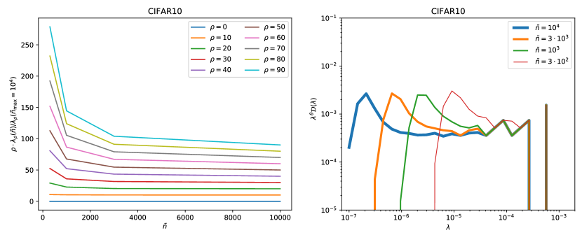
To extract the exponent a𝑎a and test this prediction for real data, we first approximate the eigenvalue equation Eq. (9) for the Student kernel with the diagonalization of its finite-dimensional Gram matrix 𝕂Ssubscript𝕂𝑆\mathbb{K}_{S} computed on a large dataset of size n~~𝑛\tilde{n}:

𝕂Sϕ¯ρλρϕ¯ρ,similar-tosubscript𝕂𝑆subscript¯italic-ϕ𝜌subscript𝜆𝜌subscript¯italic-ϕ𝜌\mathbb{K}_{S}\underline{\phi}_{\rho}\sim\lambda_{\rho}\underline{\phi}_{\rho}, (13)

where now we have n~~𝑛\tilde{n} eigenvalues λ1λn~subscript𝜆1subscript𝜆~𝑛\lambda_{1}\geq\cdots\geq\lambda_{\tilde{n}} and the eigenvectors ϕ¯ρsubscript¯italic-ϕ𝜌\underline{\phi}_{\rho} are n~~𝑛\tilde{n}-dimensional eigenvectors. Computing this diagonalization for a given training set is referred to (uncentered) kernel PCA. This procedure is a discretized version of Eq. (10) and yields only an approximation to the largest n~~𝑛\tilde{n} eigenvalues of the kernel, that are exactly recovered as n~~𝑛\tilde{n}\to\infty (in Fig. 9 in Appendix J we show that the eigenvalues of the Gram matrix converge when n~~𝑛\tilde{n} increases, and that their density displays the power-law behavior that one can extract from the kernel operator with a uniform distribution p(x¯)𝑝¯𝑥p(\underline{x})). The coefficient qρsubscript𝑞𝜌q_{\rho} is then estimated by the scalar products (Z¯ϕ¯ρ)¯𝑍subscript¯italic-ϕ𝜌\left(\underline{Z}\cdot\underline{\phi}_{\rho}\right), where Z¯=(Z(x¯1),,Z(x¯n~))¯𝑍𝑍subscript¯𝑥1𝑍subscript¯𝑥~𝑛\underline{Z}=(Z(\underline{x}_{1}),\cdots,Z(\underline{x}_{\tilde{n}})) is the vector of the target function’s values on the train set.

Finally, we approximate Eq. (12) as:

ρ=nn~(Z¯ϕ¯ρ)2.superscriptsubscript𝜌𝑛~𝑛superscript¯𝑍subscript¯italic-ϕ𝜌2\sum_{\rho=n}^{\tilde{n}}\left(\underline{Z}\cdot\underline{\phi}_{\rho}\right)^{2}. (14)

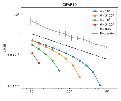
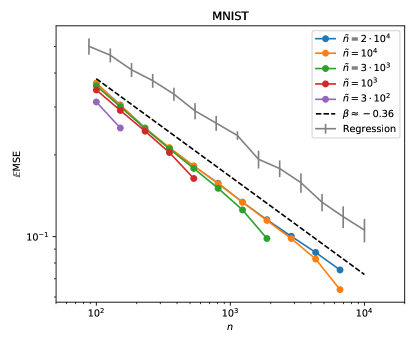
This quantity is plotted in Fig. 3, where we show that it correlates remarkably well with the true learning curve. Fitting these cumulative curves whose exponent is 1a1𝑎1-a for asymptotically large n~~𝑛\tilde{n} (here we plotted several curves for growing n~~𝑛\tilde{n}) we extract an exponent aMNIST=1.36subscript𝑎MNIST1.36a_{\mathrm{MNIST}}=1.36 leading to β^MNIST0.36subscript^𝛽MNIST0.36\hat{\beta}_{\mathrm{MNIST}}\approx 0.36 and aCIFAR10=1.07subscript𝑎CIFAR101.07a_{\mathrm{CIFAR10}}=1.07 leading to β^CIFAR100.07subscript^𝛽CIFAR100.07\hat{\beta}_{\mathrm{CIFAR10}}\approx 0.07 that are very close to the exponents that we measured in Section 3.
Refer to caption
Refer to caption
Figure 3: Several measures of the learning curves for MNIST (left) and CIFAR10 (right). In every plot, the gray solid line is the numerical evaluation of the generalization error (shifted for clarity). Colored lines are computed using Eq. (14) for several values of n~~𝑛\tilde{n}, and the dashed black line is the a fit of the power-law decay with which we extract the predicted exponents β^MNIST0.36subscript^𝛽MNIST0.36\hat{\beta}_{\mathrm{MNIST}}\approx 0.36 and β^CIFAR100.07subscript^𝛽CIFAR100.07\hat{\beta}_{\mathrm{CIFAR10}}\approx 0.07.

Support for the genericity of Eq. (12) can be obtained from the recent paper [11], where the authors derived a formula for the generalization error based on the decomposition of the target function on the eigenbasis of the kernel. The formula is derived with uncontrolled approximations, but applies to a generic target function (or ensembles thereof) and a generic data point distribution p(x¯)𝑝¯𝑥p(\underline{x}), and matches well their numerical experiments. In Appendix I we show that the asymptotic limit (large n𝑛n) of their formula yields Eq. (12). Furthermore, Eq.7 is recovered if a power-law decay of the coefficient of the true function in the eigenbasis of the kernel is assumed- thus generalizing our result to non-Gaussian data.

7 Effective dimension of real data
Refer to caption
Figure 4: Average distance from one point to its nearest neighbor as a function of the dataset size n𝑛n. (Left) For random points on d𝑑d-dimensional hypersphere, δminn1/dsimilar-todelimited-⟨⟩subscript𝛿minsuperscript𝑛1𝑑\left<\delta_{\mathrm{min}}\right>\sim n^{-\nicefrac{{1}}{{d}}}. Colored solid curves are found numerically, dashed lines are the theoretical asymptotic prediction and the gray lines are numerical fit (we fitted only starting from n6000𝑛6000n\approx 6000 to reduce finite size effects, and the fit have been rescaled to match the data at n=10𝑛10n=10). The larger d𝑑d, the stronger the preasymptotic effects (a larger n𝑛n is needed to observe the predicted scaling). (Right) Comparison between random data on 151515- and 353535-dimensional hyperspheres and the MNIST, CIFAR10 datasets. According to this definition of effective dimension, MNIST live on a 151515-dimensional manifold and CIFAR10 on a 353535-dimensional one. Data have been rescaled along the y𝑦y-axis for ease of comparison.

Both our predictions and empirical observations support rather large values of β𝛽\beta. From a Gaussian random process point of view, it is surprising: the exponent β𝛽\beta avoids the curse of dimensionality only if the smoothness of the Teacher is of the order of the data dimension. If these observations were to hold true also for real data, it would seem to imply that MNIST and CIFAR10 must be hundreds or thousands of times differentiable! However, there is a simple catch: real data actually live on a manifold of much lower dimensionality. Above we have argued that the quantity that governs the asymptotic learning curve is the typical distance δminsubscript𝛿min\delta_{\mathrm{min}} between neighboring points in the training set. A simple way to measure the effective dimension deffsubscript𝑑effd_{\mathrm{eff}} of real data consists then in plotting the (asymptotic) dependence of δminsubscript𝛿min\delta_{\mathrm{min}} on the number of points n𝑛n in a random subset of the dataset, and fitting

δminn1/deff.similar-tosubscript𝛿minsuperscript𝑛1subscript𝑑eff\delta_{\mathrm{min}}\sim n^{-\nicefrac{{1}}{{d_{\mathrm{eff}}}}}. (15)

In Fig. 4 (right) we show that for MNIST and CIFAR10 there is indeed a power-law relation linking δminsubscript𝛿min\delta_{\mathrm{min}} to n𝑛n, and that the effective dimension extracted this way is much smaller than the embedding dimension of the datasets:

deffMNIST15superscriptsubscript𝑑effMNIST15\displaystyle d_{\mathrm{eff}}^{\mathrm{MNIST}}\approx 15 784=dMNIST,much-less-thanabsent784superscript𝑑MNIST\displaystyle\ll 784=d^{\mathrm{MNIST}}, (16)
deffCIFAR1035superscriptsubscript𝑑effCIFAR1035\displaystyle d_{\mathrm{eff}}^{\mathrm{CIFAR10}}\approx 35 3072=dCIFAR10.much-less-thanabsent3072superscript𝑑CIFAR10\displaystyle\ll 3072=d^{\mathrm{CIFAR10}}. (17)

This measure is consistent with previous extrapolations of the intrinsic dimension of MNIST [19, 20, 22, 23].

8 Conclusion

In this work we have shown for CIFAR10 and MNIST respectively that kernel regression and classification display a power-law decay in the learning curves, quite remarkably with essentially the same exponent β𝛽\beta regardless of task and kernel — a fact yet to be explained. These exponents are much larger than β=1/d𝛽1𝑑\beta=1/d expected for Lipschitz target functions and smaller than β=1/2𝛽12\beta=1/2 expected for RKHS target functions.

This observation led us to study a Teacher-Student framework for regression in which data are modeled as Gaussian random fields of varying smoothness, in which intermediary values of β𝛽\beta are obtained. We find two regimes depending on the respective smoothness of the Teacher and Student kernels. If the student is smooth enough — i.e. it puts a sufficiently low prior on high frequency components — then β𝛽\beta is entirely controlled by the Teacher. We obtain that the smoothness index must scale with the dimension for β𝛽\beta to be finite as d𝑑d\rightarrow\infty, recovering the curse of dimensionality.

In our calculations, the dimension enters as the parameter relating the number of points to the nearest-neighbor distance δn1/dsimilar-to𝛿superscript𝑛1𝑑\delta\sim n^{-1/d}. Thus in practice the parameter d𝑑d considered should be the effective dimension deffsubscript𝑑𝑒𝑓𝑓d_{eff} of the data, which is much smaller than the number of pixels for MNIST and CIFAR data. It explains why β𝛽\beta is not very small in these cases.

Finally, for Gaussian fields our result is equivalent to the statement that β𝛽\beta is governed by the power of the true function past the first nsimilar-toabsent𝑛\sim n eigenvectors of the kernel. We test this more general idea both for CIFAR and MNIST and find that it correctly predicts β𝛽\beta. Understanding what controls this power in a general setting (which include the effective dimension of the data and presumably a generalized quantity characterizing smoothness) thus appears necessary to understand how many data are required to learn a task.

Acknowledgments

We acknowledge G. Biroli, C. Hongler and F. Gabriel for the discussions that stimulated this work, and we thank S. d’Ascoli, A. Jacot, C. Pehlevan, L. Sagun and M.L. Stein for discussions. This work was partially supported by the grant from the Simons Foundation (#454953 Matthieu Wyart). M.W. thanks the Swiss National Science Foundation for support under Grant No. 200021-165509.

References

  • [1] Joel Hestness, Sharan Narang, Newsha Ardalani, Gregory Frederick Diamos, Heewoo Jun, Hassan Kianinejad, Md. Mostofa Ali Patwary, Yang Yang, and Yanqi Zhou. Deep learning scaling is predictable, empirically. CoRR, abs/1712.00409, 2017.
  • [2] Arthur Jacot, Franck Gabriel, and Clément Hongler. Neural tangent kernel: Convergence and generalization in neural networks. In Advances in neural information processing systems, pages 8571–8580, 2018.
  • [3] Joan Bruna and Stéphane Mallat. Invariant scattering convolution networks. IEEE transactions on pattern analysis and machine intelligence, 35(8):1872–1886, 2013.
  • [4] Sanjeev Arora, Simon S Du, Wei Hu, Zhiyuan Li, Ruslan Salakhutdinov, and Ruosong Wang. On exact computation with an infinitely wide neural net. arXiv preprint arXiv:1904.11955, 2019.
  • [5] Ulrike von Luxburg and Olivier Bousquet. Distance-based classification with lipschitz functions. Journal of Machine Learning Research, 5(Jun):669–695, 2004.
  • [6] Francis Bach. Breaking the curse of dimensionality with convex neural networks. The Journal of Machine Learning Research, 18(1):629–681, 2017.
  • [7] Alex J Smola, Bernhard Schölkopf, and Klaus-Robert Müller. The connection between regularization operators and support vector kernels. Neural networks, 11(4):637–649, 1998.
  • [8] Alessandro Rudi and Lorenzo Rosasco. Generalization properties of learning with random features. In Advances in Neural Information Processing Systems, pages 3215–3225, 2017.
  • [9] Georges Matheron. Principles of geostatistics. Economic geology, 58(8):1246–1266, 1963.
  • [10] Michael L Stein. Interpolation of spatial data: some theory for kriging. Springer Science & Business Media, 1999.
  • [11] Blake Bordelon, Abdulkadir Canatar, and Cengiz Pehlevan. Spectrum dependent learning curves in kernel regression and wide neural networks. arXiv preprint arXiv:2002.02561, 2020.
  • [12] Simon Fischer and Ingo Steinwart. Sobolev norm learning rates for regularized least-squares algorithm. arXiv preprint arXiv:1702.07254, 2017.
  • [13] Andrea Caponnetto and Ernesto De Vito. Optimal rates for the regularized least-squares algorithm. Foundations of Computational Mathematics, 7(3):331–368, 2007.
  • [14] Loucas Pillaud-Vivien, Alessandro Rudi, and Francis Bach. Statistical optimality of stochastic gradient descent on hard learning problems through multiple passes. In Advances in Neural Information Processing Systems, pages 8114–8124, 2018.
  • [15] Peter Sollich. Learning curves for gaussian processes. In Advances in neural information processing systems, pages 344–350, 1999.
  • [16] Peter Sollich. Gaussian process regression with mismatched models. In Advances in Neural Information Processing Systems, pages 519–526, 2002.
  • [17] Michael L Stein. Predicting random fields with increasing dense observations. The Annals of Applied Probability, 9(1):242–273, 1999.
  • [18] Peter Grassberger and Itamar Procaccia. Measuring the strangeness of strange attractors. Physica D: Nonlinear Phenomena, 9(1-2):189–208, 1983.
  • [19] Jose A Costa and Alfred O Hero. Learning intrinsic dimension and intrinsic entropy of high-dimensional datasets. In 2004 12th European Signal Processing Conference, pages 369–372. IEEE, 2004.
  • [20] Matthias Hein and Jean-Yves Audibert. Intrinsic dimensionality estimation of submanifolds in r d. In Proceedings of the 22nd international conference on Machine learning, pages 289–296. ACM, 2005.
  • [21] Elizaveta Levina and Peter J Bickel. Maximum likelihood estimation of intrinsic dimension. In Advances in neural information processing systems, pages 777–784, 2005.
  • [22] Alessandro Rozza, Gabriele Lombardi, Claudio Ceruti, Elena Casiraghi, and Paola Campadelli. Novel high intrinsic dimensionality estimators. Machine learning, 89(1-2):37–65, 2012.
  • [23] Elena Facco, Maria d’Errico, Alex Rodriguez, and Alessandro Laio. Estimating the intrinsic dimension of datasets by a minimal neighborhood information. Scientific reports, 7(1):12140, 2017.
  • [24] Michele Allegra, Elena Facco, Alessandro Laio, and Antonietta Mira. Clustering by the local intrinsic dimension: the hidden structure of real-world data. arXiv preprint arXiv:1902.10459, 2019.
  • [25] Bernhard Scholkopf and Alexander J Smola. Learning with kernels: support vector machines, regularization, optimization, and beyond. MIT press, 2001.
  • [26] David Saad and Sara A Solla. On-line learning in soft committee machines. Physical Review E, 52(4):4225, 1995.
  • [27] Rémi Monasson and Riccardo Zecchina. Weight space structure and internal representations: a direct approach to learning and generalization in multilayer neural networks. Physical review letters, 75(12):2432, 1995.
  • [28] Manfred Opper and David Saad. Advanced mean field methods: Theory and practice. MIT press, 2001.
  • [29] Andreas Engel and Christian Van den Broeck. Statistical mechanics of learning. Cambridge University Press, 2001.
  • [30] Jean Barbier, Florent Krzakala, Nicolas Macris, Léo Miolane, and Lenka Zdeborova. Optimal errors and phase transitions in high-dimensional generalized linear models. Proceedings of the National Academy of Sciences, 116:201802705, 03 2019.
  • [31] Marylou Gabrié, Andre Manoel, Clément Luneau, Nicolas Macris, Florent Krzakala, Lenka Zdeborová, et al. Entropy and mutual information in models of deep neural networks. In Advances in Neural Information Processing Systems, pages 1821–1831, 2018.
  • [32] Benjamin Aubin, Antoine Maillard, Florent Krzakala, Nicolas Macris, Lenka Zdeborová, et al. The committee machine: Computational to statistical gaps in learning a two-layers neural network. In Advances in Neural Information Processing Systems, pages 3223–3234, 2018.
  • [33] Silvio Franz, Sungmin Hwang, and Pierfrancesco Urbani. Jamming in multilayer supervised learning models. arXiv preprint arXiv:1809.09945, 2018.
  • [34] Christopher KI Williams and Carl Edward Rasmussen. Gaussian processes for machine learning, volume 2. MIT Press Cambridge, MA, 2006.

Appendix A Soft-margin Support Vector Machines

The kernel classification task is performed via the algorithm known as soft-margin Support Vector Machine.

We want to find a function Z^S(x¯)subscript^𝑍𝑆¯𝑥\hat{Z}_{S}(\underline{x}) such that its sign correctly predicts the label of the data. In this context we model such a function as a linear prediction after projecting the data on a feature space via x¯ϕ(x¯)¯𝑥italic-ϕ¯𝑥\underline{x}\to\phi(\underline{x}):

Z^S(x¯)=w¯ϕ¯S(x¯μ)+b,subscript^𝑍𝑆¯𝑥¯𝑤subscript¯italic-ϕ𝑆subscript¯𝑥𝜇𝑏\hat{Z}_{S}(\underline{x})=\underline{w}\cdot\underline{\phi}_{S}(\underline{x}_{\mu})+b, (18)

where w¯,b¯𝑤𝑏\underline{w},b are parameters to be learned from the training data. The kernel is related to the feature space via KS(x¯,x¯)=ϕ¯S(x¯)ϕ¯S(x¯)subscript𝐾𝑆¯𝑥superscript¯𝑥subscript¯italic-ϕ𝑆¯𝑥subscript¯italic-ϕ𝑆superscript¯𝑥K_{S}(\underline{x},\underline{x}^{\prime})=\underline{\phi}_{S}(\underline{x})\cdot\underline{\phi}_{S}(\underline{x}^{\prime}). We require that Z(x¯μ)Z^S(x¯μ)>1ξμ𝑍subscript¯𝑥𝜇subscript^𝑍𝑆subscript¯𝑥𝜇1subscript𝜉𝜇Z(\underline{x}_{\mu})\hat{Z}_{S}(\underline{x}_{\mu})>1-\xi_{\mu} for all training points. Ideally we want to have some large margins 1ξμ=11subscript𝜉𝜇11-\xi_{\mu}=1, but we allow some of them to be smaller by introducing the slack variables ξμsubscript𝜉𝜇\xi_{\mu} and penalizing large values. To achieve this the following constrained minimization is performed:

minw¯,b,ξ¯12w¯2+CμξμsubjectedtoμZ(x¯μ)[w¯ϕ¯S(x¯μ)+b]1ξμ,ξμ0.formulae-sequencesubscript¯𝑤𝑏¯𝜉12superscriptnorm¯𝑤2𝐶subscript𝜇subscript𝜉𝜇subjectedtofor-all𝜇𝑍subscript¯𝑥𝜇delimited-[]¯𝑤subscript¯italic-ϕ𝑆subscript¯𝑥𝜇𝑏1subscript𝜉𝜇subscript𝜉𝜇0\min_{\underline{w},b,\underline{\xi}}\frac{1}{2}|\!|\underline{w}|\!|^{2}+C\sum_{\mu}\xi_{\mu}\quad\mathrm{subjected\ to}\quad\forall\mu\ Z(\underline{x}_{\mu})\left[\underline{w}\cdot\underline{\phi}_{S}(\underline{x}_{\mu})+b\right]\geq 1-\xi_{\mu},\ \xi_{\mu}\geq 0. (19)

This problem can be expressed in a dual formulation as

mina¯12a¯Sa¯μ=1naμsubjectedtoZ¯a¯=0, 0aμC,formulae-sequencesubscript¯𝑎12¯𝑎subscript𝑆¯𝑎superscriptsubscript𝜇1𝑛subscript𝑎𝜇subjectedto¯𝑍¯𝑎0 0subscript𝑎𝜇𝐶\min_{\underline{a}}\frac{1}{2}\underline{a}\cdot\mathbb{Q}_{S}\underline{a}-\sum_{\mu=1}^{n}a_{\mu}\quad\mathrm{subjected\ to}\quad\underline{Z}\cdot\underline{a}=0,\ 0\leq a_{\mu}\leq C, (20)

where S,μ,ν=Z(x¯μ)Z(x¯ν)KS(x¯μ,x¯ν)subscript𝑆𝜇𝜈𝑍subscript¯𝑥𝜇𝑍subscript¯𝑥𝜈subscript𝐾𝑆subscript¯𝑥𝜇subscript¯𝑥𝜈\mathbb{Q}_{S,\mu,\nu}=Z(\underline{x}_{\mu})Z(\underline{x}_{\nu})K_{S}(\underline{x}_{\mu},\underline{x}_{\nu}) and Z¯¯𝑍\underline{Z} is the vector of the labels of the training points. Here C𝐶C (=104absentsuperscript104=10^{4} in our simulations) controls the trade-off between minimizing the training error and maximizing the margins 1ξμ1subscript𝜉𝜇1-\xi_{\mu}. For the details we refer to [25]. If a¯superscript¯𝑎\underline{a}^{\star} is the solution to the minimization problem, than

w¯=μaμϕ¯S(x¯μ),superscript¯𝑤subscript𝜇superscriptsubscript𝑎𝜇subscript¯italic-ϕ𝑆subscript¯𝑥𝜇\displaystyle\underline{w}^{\star}=\sum_{\mu}a_{\mu}^{\star}\underline{\phi}_{S}(\underline{x}_{\mu}), (21)
b=Z(x¯μ)νaνyνKS(x¯μ,x¯ν)foranyμsuchthataμ<C.formulae-sequencesuperscript𝑏𝑍subscript¯𝑥𝜇subscript𝜈subscript𝑎𝜈subscript𝑦𝜈subscript𝐾𝑆subscript¯𝑥𝜇subscript¯𝑥𝜈forany𝜇suchthatsubscript𝑎𝜇𝐶\displaystyle b^{\star}=Z(\underline{x}_{\mu})-\sum_{\nu}a_{\nu}y_{\nu}K_{S}(\underline{x}_{\mu},\underline{x}_{\nu})\quad\mathrm{for\ any}\ \mu\ \mathrm{such\ that}\ a_{\mu}<C. (22)

The predicted label for unseen data points is then

sign(Z^S(x¯))=sign(μZ(x¯μ)aμKS(x¯μ,x¯)+b)signsubscript^𝑍𝑆¯𝑥signsubscript𝜇𝑍subscript¯𝑥𝜇subscript𝑎𝜇subscript𝐾𝑆subscript¯𝑥𝜇¯𝑥superscript𝑏\mathrm{sign}(\hat{Z}_{S}(\underline{x}))=\mathrm{sign}(\sum_{\mu}Z(\underline{x}_{\mu})a_{\mu}K_{S}(\underline{x}_{\mu},\underline{x})+b^{\star}) (23)

The generalization error is now defined as the probability that an unseen image has a predicted label different from the true one, and such a probability is again estimated as an average over a test set with ntestsubscript𝑛testn_{\mathrm{test}} elements:

Error=1ntestμ=1ntestθ[sign(Z^S(x¯μ))Z(x¯μ)].Error1subscript𝑛testsuperscriptsubscript𝜇1subscript𝑛test𝜃delimited-[]signsubscript^𝑍𝑆subscript¯𝑥𝜇𝑍subscript¯𝑥𝜇\mathrm{Error}=\frac{1}{n_{\mathrm{test}}}\sum_{\mu=1}^{n_{\mathrm{test}}}\theta\left[-\mathrm{sign}\left(\hat{Z}_{S}(\underline{x}_{\mu})\right)Z(\underline{x}_{\mu})\right]. (24)

Appendix B Different kernel variances

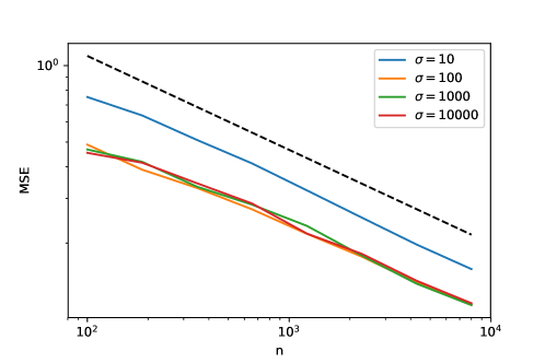
In Fig. 5 we show the learning curves for kernel regression on the MNIST (parity) dataset — the same setting as in Fig. 1 (a). Several Laplace kernels of varying variance σ𝜎\sigma are used. The variance ranges several orders of magnitude and the learning curves all decay with the same exponent, although for σ=10𝜎10\sigma=10 the algorithm achieves suboptimal performance and the test errors are increased by some factor.
Refer to caption
Figure 5: Learning curves for kernel regression on the MNIST dataset. Regression is performed with several Laplace kernels of varying variance σ𝜎\sigma ranging from σ=10𝜎10\sigma=10 to σ=10000𝜎10000\sigma=10000.

Appendix C Different choice of kernel variances

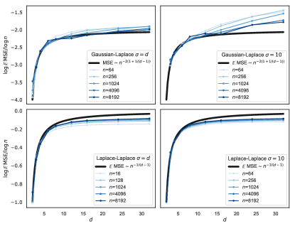
In Fig. 6 we show the learning curves for the Teacher-Student kernel regression problem, with a Student kernel that is always Laplace and a Teacher that can be either Gaussian or Laplace. We show how the test error decays with the size of the training dataset and how the asymptotic exponent depends on the spatial dimension. Every experiment is run with two different choices of the kernel variances: in one case σT=σS=dsubscript𝜎𝑇subscript𝜎𝑆𝑑\sigma_{T}=\sigma_{S}=d and in the other σT=σS=10subscript𝜎𝑇subscript𝜎𝑆10\sigma_{T}=\sigma_{S}=10. We observed that scaling the variances with the spatial dimension leads faster to the results that we predicted in this paper, but overall the choice has little effect on the exponents (both tend towards the prediction as the dataset size is increased).
Refer to caption
Refer to caption
Figure 6: In these plots we show the results for the Teacher-Student kernel regression. The Student is always a Laplace kernel, the Teacher is either Gaussian or Laplace. The four plots on the left depict the mean-square error against the size of the dataset for different spatial dimensions of the data, those on the right show the fitted asymptotic exponent against the spatial dimension for different dataset sizes. For every case we show both the the results for σT=σS=dsubscript𝜎𝑇subscript𝜎𝑆𝑑\sigma_{T}=\sigma_{S}=d and σT=σS=10subscript𝜎𝑇subscript𝜎𝑆10\sigma_{T}=\sigma_{S}=10.
Refer to caption
Refer to caption
Refer to caption
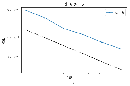
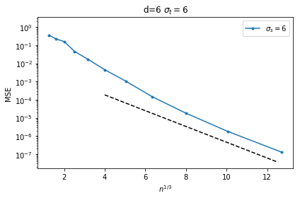
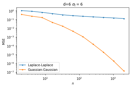
Figure 7: Left: The test error of a Laplace Teacher (αT=d+1subscript𝛼𝑇𝑑1\alpha_{T}=d+1) with a Gaussian Student (αS=subscript𝛼𝑆\alpha_{S}=\infty) decays as a power law with the predicted exponent β=1dmin(1,)=16𝛽1𝑑116\beta=\frac{1}{d}\min(1,\infty)=\frac{1}{6} in d=6𝑑6d=6 dimensions. Center: When both the Teacher and the Student are Gaussian the test error decays faster than any power law as the number n𝑛n of data is increased. This plot confirm this by showing that the logarithm of the test error decays linearly as a function of n13superscript𝑛13n^{\frac{1}{3}}. Right: Comparison between the learning curves for the cases where both kernels are either Laplace (top blue line) or Gaussian (bottom orange line). While the former decays algebraically with the predicted exponent, the latter decays exponentially, in agreement with the prediction β=𝛽\beta=\infty found within our framework. In all these plots we have taken the variances of both the Teacher and Student kernels to be equal to the dimension d=6𝑑6d=6.

Appendix D Gaussian Students

In this appendix we present the learning curves of Gaussian Students: the Fourier transform of these kernels decays faster than any power law and one can effectively consider αS=subscript𝛼𝑆\alpha_{S}=\infty. If the Teacher is Laplace (αT=d+1subscript𝛼𝑇𝑑1\alpha_{T}=d+1) then the predicted exponent is finite and takes the values β=1dmin(αTd,2αS)=1dmin(1,)=1d𝛽1𝑑subscript𝛼𝑇𝑑2subscript𝛼𝑆1𝑑11𝑑\beta=\frac{1}{d}\min(\alpha_{T}-d,2\alpha_{S})=\frac{1}{d}\min(1,\infty)=\frac{1}{d}. Such a case is displayed in Fig. 7 (left) in dimension d=6𝑑6d=6. However, if we consider the Teacher to be Gaussian as well, then the predicted exponent would be β=1dmin(,)=𝛽1𝑑\beta=\frac{1}{d}\min(\infty,\infty)=\infty. This case corresponds to Fig. 7 (center): the test errors decays faster than a power law. In Fig. 7 (right) we compare the case where both kernels are Gaussian to the case where both kernels are Laplace: while the latter decays as a power law, the former decays much faster.

Appendix E Matérn Teachers

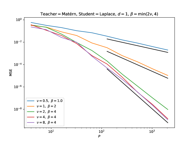
To further test the applicability of our theory, we show here some numerical simulations for a Teacher kernel that is a Matérn covariance function and a Laplace kernel as student. We ran the simulations in 1d: the data points are sampled uniformly on a 1-dimensional circle embedded in 2superscript2\mathbb{R}^{2}. Matérn kernels are parametrized by a parameter ν>0𝜈0\nu>0:

KT(x¯)=21νΓ(ν)zν𝒦ν(z),subscript𝐾𝑇¯𝑥superscript21𝜈Γ𝜈superscript𝑧𝜈subscript𝒦𝜈𝑧K_{T}(\underline{x})=\frac{2^{1-\nu}}{\Gamma(\nu)}z^{\nu}\mathcal{K}_{\nu}(z), (25)

where z=2νx¯σ𝑧2𝜈norm¯𝑥𝜎z=\sqrt{2\nu}\frac{|\!|\underline{x}|\!|}{\sigma} (σ𝜎\sigma being the kernel variance), ΓΓ\Gamma is the gamma function and 𝒦νsubscript𝒦𝜈\mathcal{K}_{\nu} is the Bessel function of the second kind with parameter ν𝜈\nu. Interestingly we recover the Laplace kernel for ν=1/2𝜈12\nu=\nicefrac{{1}}{{2}} and the Gaussian kernel for ν=𝜈\nu=\infty. As one can find in e.g. [34], the exponent αTsubscript𝛼𝑇\alpha_{T} that governs the decay at high frequency of this kernels is αT=d+2νsubscript𝛼𝑇𝑑2𝜈\alpha_{T}=d+2\nu. Varying ν𝜈\nu we can change the smoothness of the target function.

For d=1𝑑1d=1 our prediction for the learning curve exponent β𝛽\beta is

β=1dmin(αTd,2αS)=min(2ν,4).𝛽1𝑑subscript𝛼𝑇𝑑2subscript𝛼𝑆2𝜈4\beta=\frac{1}{d}\min(\alpha_{T}-d,2\alpha_{S})=\min(2\nu,4). (26)

In Fig. 8 we verify that our prediction matches the numerical results.
Refer to caption
Figure 8: Mean-squared error for Matérn Teacher kernels and Laplace students. The variance of the kernels is equal to 222 for all the curves.

Appendix F Proof of theorem

We prove here Theorem 5:

Theorem 1 Let K~T(w¯)=cTw¯αT+o(w¯αT)subscript~𝐾𝑇¯𝑤subscript𝑐𝑇superscriptnorm¯𝑤subscript𝛼𝑇𝑜superscriptnorm¯𝑤subscript𝛼𝑇\tilde{K}_{T}(\underline{w})=c_{T}|\!|\underline{w}|\!|^{-\alpha_{T}}+o\left(|\!|\underline{w}|\!|^{-\alpha_{T}}\right) and K~S(w¯)=cSw¯αS+o(w¯αS)subscript~𝐾𝑆¯𝑤subscript𝑐𝑆superscriptnorm¯𝑤subscript𝛼𝑆𝑜superscriptnorm¯𝑤subscript𝛼𝑆\tilde{K}_{S}(\underline{w})=c_{S}|\!|\underline{w}|\!|^{-\alpha_{S}}+o\left(|\!|\underline{w}|\!|^{-\alpha_{S}}\right) as w¯norm¯𝑤|\!|\underline{w}|\!|\to\infty, where K~T(w¯)subscript~𝐾𝑇¯𝑤\tilde{K}_{T}(\underline{w}) and K~S(w¯)subscript~𝐾𝑆¯𝑤\tilde{K}_{S}(\underline{w}) are the Fourier transforms of the kernels KT(x¯)subscript𝐾𝑇¯𝑥K_{T}(\underline{x}), KS(x¯)subscript𝐾𝑆¯𝑥K_{S}(\underline{x}) respectively, assumed to be positive definite. We assume that K~T(w¯)subscript~𝐾𝑇¯𝑤\tilde{K}_{T}(\underline{w}) and K~S(w¯)subscript~𝐾𝑆¯𝑤\tilde{K}_{S}(\underline{w}) have a finite limit as w¯0norm¯𝑤0|\!|\underline{w}|\!|\to 0 and that K(0¯)<𝐾¯0K(\underline{0})<\infty. Then,

𝔼MSE=nβ+o(nβ)withβ=1dmin(αTd,2αS).formulae-sequence𝔼MSEsuperscript𝑛𝛽𝑜superscript𝑛𝛽with𝛽1𝑑subscript𝛼𝑇𝑑2subscript𝛼𝑆\mathbb{E}\,\mathrm{MSE}=n^{-\beta}+o\left(n^{-\beta}\right)\quad\mathrm{with}\quad\beta=\frac{1}{d}\min(\alpha_{T}-d,2\alpha_{S}). (27)

Moreover, in the case of a Gaussian kernel the result holds valid if we take the corresponding exponent to be α=𝛼\alpha=\infty.

Proof.

Our strategy is to compute how the mean-square test error scales with distance δ𝛿\delta between two nearest neighbors on the d𝑑d-dimensional regular lattice. At the end, we will use the fact that δn1/dproportional-to𝛿superscript𝑛1𝑑\delta\propto n^{-\nicefrac{{1}}{{d}}}, where n𝑛n is the number of sampled points on the lattice.

We denote by F~(w¯)~𝐹¯𝑤\tilde{F}(\underline{w}) the Fourier transform of a function F:𝒱:𝐹𝒱F:\mathcal{V}\to\mathbb{R}:

F~(w¯)=Ld/2𝒱dx¯eiw¯x¯F(x¯),wherew¯𝕃2πLd,formulae-sequence~𝐹¯𝑤superscript𝐿𝑑2subscript𝒱differential-d¯𝑥superscript𝑒𝑖¯𝑤¯𝑥𝐹¯𝑥where¯𝑤𝕃2𝜋𝐿superscript𝑑\displaystyle\tilde{F}(\underline{w})=L^{-\nicefrac{{d}}{{2}}}\int_{\mathcal{V}}\mathrm{d}\underline{x}\,e^{-i\underline{w}\cdot\underline{x}}F(\underline{x}),\quad\mathrm{where}\ \underline{w}\in\mathbb{L}\equiv\frac{2\pi}{L}\mathbb{Z}^{d}, (28)
F(x¯)=Ld/2w¯𝕃eiw¯x¯F~(w¯).𝐹¯𝑥superscript𝐿𝑑2subscript¯𝑤𝕃superscript𝑒𝑖¯𝑤¯𝑥~𝐹¯𝑤\displaystyle F(\underline{x})=L^{-\nicefrac{{d}}{{2}}}\sum_{\underline{w}\in\mathbb{L}}e^{i\underline{w}\cdot\underline{x}}\tilde{F}(\underline{w}). (29)

If Z𝒩(0,K)similar-to𝑍𝒩0𝐾Z\sim\mathcal{N}(0,K) is a Gaussian field with translation-invariant covariance K𝐾K then by definition

𝔼Z(x¯)Z(x¯)=K(x¯x¯).𝔼𝑍¯𝑥𝑍superscript¯𝑥𝐾¯𝑥superscript¯𝑥\mathbb{E}Z(\underline{x})Z(\underline{x}^{\prime})=K(\underline{x}-\underline{x}^{\prime}). (30)

Properties of the Fourier transform of a Gaussian field:

K~(w¯)=K~(w¯),~𝐾¯𝑤~𝐾¯𝑤\displaystyle\tilde{K}(\underline{w})=\tilde{K}(-\underline{w})\in\mathbb{R}, (31)
𝔼Z~(w¯)=0,𝔼~𝑍¯𝑤0\displaystyle\mathbb{E}\tilde{Z}(\underline{w})=0, (32)
𝔼Z~(w¯)Z~(w¯)¯=Ld/2δw¯w¯K~(w¯).𝔼~𝑍¯𝑤¯~𝑍superscript¯𝑤superscript𝐿𝑑2subscript𝛿¯𝑤superscript¯𝑤~𝐾¯𝑤\displaystyle\mathbb{E}\tilde{Z}(\underline{w})\overline{\tilde{Z}(\underline{w}^{\prime})}=L^{\nicefrac{{d}}{{2}}}\delta_{\underline{w}\underline{w}^{\prime}}\tilde{K}(\underline{w}). (33)

Eq. (31) comes from the fact that K(x¯)𝐾¯𝑥K(\underline{x}) is an even, real-valued function. The real and imaginary parts of Z~(w¯)~𝑍¯𝑤\tilde{Z}(\underline{w}) are Gaussian random variables. They are all independent except that Z~(w¯)=Z~(w¯)¯~𝑍¯𝑤¯~𝑍¯𝑤\tilde{Z}(-\underline{w})=\overline{\tilde{Z}(\underline{w})}. Eq. (33) follows from the fact that Z(x¯)𝑍¯𝑥Z(\underline{x}) and K(x¯)𝐾¯𝑥K(\underline{x}) are L𝐿L-periodic functions, and therefore eiw¯x¯K~(w¯)superscript𝑒𝑖¯𝑤¯𝑥~𝐾¯𝑤e^{i\underline{w}\cdot\underline{x}}\tilde{K}(\underline{w}) is the Fourier transform of K(+x¯)K(\cdot+\underline{x}) if w¯2πLd¯𝑤2𝜋𝐿superscript𝑑\underline{w}\in\frac{2\pi}{L}\mathbb{Z}^{d}. #

The solution Eq. (3) for kernel regression has two interpretations. In Section 4 we introduced it as the quantity that minimizes a quadratic error, but it can also be seen as the maximum-a-posteriori (MAP) estimation of another formulation of the problem [34]. The field Z(x¯)𝑍¯𝑥Z(\underline{x}) is assumed to be drawn from a Gaussian distribution with covariance function KS(x¯)subscript𝐾𝑆¯𝑥K_{S}(\underline{x}): KSsubscript𝐾𝑆K_{S} therefore plays a role in the prior distribution of the data Z¯=(Z(x¯μ)μ=1n)¯𝑍𝑍superscriptsubscriptsubscript¯𝑥𝜇𝜇1𝑛\underline{Z}=(Z(\underline{x}_{\mu})_{\mu=1}^{n}). Inference about the value of the field Z^S(x¯)subscript^𝑍𝑆¯𝑥\hat{Z}_{S}(\underline{x}) at another location is then performed by maximizing its posterior distribution,

Z^S(x¯)argmax𝒫(Z(x¯)|Z¯).subscript^𝑍𝑆¯𝑥argmax𝒫conditional𝑍¯𝑥¯𝑍\hat{Z}_{S}(\underline{x})\equiv\mathrm{arg\ max}\ \mathcal{P}\left(Z(\underline{x})|\underline{Z}\right). (34)

Such a posterior distribution is Gaussian, and its mean — and therefore also the value that maximizes the probability — is exactly Eq. (3):

Z^S(x¯)=k¯S(x¯)𝕂S1Z¯,subscript^𝑍𝑆¯𝑥subscript¯𝑘𝑆¯𝑥superscriptsubscript𝕂𝑆1¯𝑍\hat{Z}_{S}(\underline{x})=\underline{k}_{S}(\underline{x})\cdot\mathbb{K}_{S}^{-1}\underline{Z}, (35)

where where Z¯=(Z(x¯μ))μ=1n¯𝑍superscriptsubscript𝑍subscript¯𝑥𝜇𝜇1𝑛\underline{Z}=\left(Z(\underline{x}_{\mu})\right)_{\mu=1}^{n} are the training data, k¯S(x¯)=(KS(x¯μ,x¯))μ=1nsubscript¯𝑘𝑆¯𝑥superscriptsubscriptsubscript𝐾𝑆subscript¯𝑥𝜇¯𝑥𝜇1𝑛\underline{k}_{S}(\underline{x})=\left(K_{S}(\underline{x}_{\mu},\underline{x})\right)_{\mu=1}^{n} and 𝕂S=(KS(x¯μ,x¯ν))μ,ν=1nsubscript𝕂𝑆superscriptsubscriptsubscript𝐾𝑆subscript¯𝑥𝜇subscript¯𝑥𝜈𝜇𝜈1𝑛\mathbb{K}_{S}=\left(K_{S}(\underline{x}_{\mu},\underline{x}_{\nu})\right)_{\mu,\nu=1}^{n} is the Gram matrix, that is invertible since the kernel KSsubscript𝐾𝑆K_{S} is assumed to be positive definite. By Fourier transforming this relation we find

Z~S(w¯)=Z~(w¯)K~S(w¯)K~S(w¯),subscript~𝑍𝑆¯𝑤superscript~𝑍¯𝑤subscript~𝐾𝑆¯𝑤superscriptsubscript~𝐾𝑆¯𝑤\tilde{Z}_{S}(\underline{w})=\tilde{Z}^{\star}(\underline{w})\frac{\tilde{K}_{S}(\underline{w})}{\tilde{K}_{S}^{\star}(\underline{w})}, (36)

where we have defined F(w¯)n¯dF(w¯+2πn¯δ)superscript𝐹¯𝑤subscript¯𝑛superscript𝑑𝐹¯𝑤2𝜋¯𝑛𝛿F^{\star}(\underline{w})\equiv\sum_{\underline{n}\in\mathbb{Z}^{d}}F\left(\underline{w}+\frac{2\pi\underline{n}}{\delta}\right) for a generic function F𝐹F.

Another way to reach Eq. (36) is to consider that we are observing the quantities

Z~(w¯)δdLd/2x¯latticeeiw¯x¯Z(x¯)n¯dZ~(w¯+2πn¯δ).superscript~𝑍¯𝑤superscript𝛿𝑑superscript𝐿𝑑2subscript¯𝑥latticesuperscript𝑒𝑖¯𝑤¯𝑥𝑍¯𝑥subscript¯𝑛superscript𝑑~𝑍¯𝑤2𝜋¯𝑛𝛿\tilde{Z}^{\star}(\underline{w})\equiv\delta^{d}L^{-\nicefrac{{d}}{{2}}}\sum_{\underline{x}\in\mathrm{lattice}}e^{-i\underline{w}\cdot\underline{x}}Z(\underline{x})\equiv\sum_{\underline{n}\in\mathbb{Z}^{d}}\tilde{Z}\left(\underline{w}+\frac{2\pi\underline{n}}{\delta}\right). (37)

Given that we know the prior distribution of the Fourier components on the right-hand side in Eq. (37), we can infer their posterior distribution once their sums are constrained by the value of Z~(w¯)superscript~𝑍¯𝑤\tilde{Z}^{\star}(\underline{w}), and it is straightforward to see that we recover Eq. (36).

The mean-square error can then be written using the Parseval-Plancherel identity,

𝔼MSE=Ld𝔼𝒱dx¯[Z(x¯)Z^S(x¯)]2=Ld𝔼w¯𝕃|Z~(w¯)Z~(w¯)K~S(w¯)K~S(w¯)|2.𝔼MSEsuperscript𝐿𝑑𝔼subscript𝒱differential-d¯𝑥superscriptdelimited-[]𝑍¯𝑥subscript^𝑍𝑆¯𝑥2superscript𝐿𝑑𝔼subscript¯𝑤𝕃superscript~𝑍¯𝑤superscript~𝑍¯𝑤subscript~𝐾𝑆¯𝑤superscriptsubscript~𝐾𝑆¯𝑤2\mathbb{E}\,\mathrm{MSE}=L^{-d}\mathbb{E}\int_{\mathcal{V}}\mathrm{d}\underline{x}\,[Z(\underline{x})-\hat{Z}_{S}(\underline{x})]^{2}=L^{-d}\mathbb{E}\sum_{\underline{w}\in\mathbb{L}}\left|\tilde{Z}(\underline{w})-\tilde{Z}^{\star}(\underline{w})\frac{\tilde{K}_{S}(\underline{w})}{\tilde{K}_{S}^{\star}(\underline{w})}\right|^{2}. (38)

By taking the expectation value with respect to the Teacher and using Eq. (31)-Eq. (33) we can write the mean-square error as

𝔼MSE=Ld𝔼w¯𝕃[Z~(w¯)Z~(w¯)¯2Z~(w¯)Z~(w¯)¯K~S(w¯)K~S(w¯)+Z~(w¯)Z~(w¯)¯K~S2(w¯)K~S2(w¯)]==Ld𝔼w¯𝕃Z~(w¯)Z~(w¯)¯2K~S(w¯)K~S(w¯)n¯dZ~(w¯)Z~(w¯+2πn¯δ)¯++K~S2(w¯)K~S2(w¯)n¯,n¯dZ~(w¯+2πn¯δ)Z~(w¯+2πn¯δ)¯==Ld/2w¯𝕃K~T(w¯)2K~S(w¯)K~S(w¯)K~T(w¯)+K~S2(w¯)K~S2(w¯)n¯dK~T(w¯+2πn¯δ)==Ld/2w¯𝕃K~T(w¯)2[K~TK~S](w¯)K~S(w¯)+K~T(w¯)[K~S2](w¯)K~S(w¯)2,𝔼MSEsuperscript𝐿𝑑𝔼subscript¯𝑤𝕃delimited-[]~𝑍¯𝑤¯~𝑍¯𝑤2~𝑍¯𝑤¯superscript~𝑍¯𝑤subscript~𝐾𝑆¯𝑤superscriptsubscript~𝐾𝑆¯𝑤superscript~𝑍¯𝑤¯superscript~𝑍¯𝑤superscriptsubscript~𝐾𝑆2¯𝑤superscriptsuperscriptsubscript~𝐾𝑆2¯𝑤superscript𝐿𝑑𝔼subscript¯𝑤𝕃~𝑍¯𝑤¯~𝑍¯𝑤2subscript~𝐾𝑆¯𝑤superscriptsubscript~𝐾𝑆¯𝑤subscript¯𝑛superscript𝑑~𝑍¯𝑤¯~𝑍¯𝑤2𝜋¯𝑛𝛿superscriptsubscript~𝐾𝑆2¯𝑤superscriptsuperscriptsubscript~𝐾𝑆2¯𝑤subscript¯𝑛superscript¯𝑛superscript𝑑~𝑍¯𝑤2𝜋¯𝑛𝛿¯~𝑍¯𝑤2𝜋superscript¯𝑛𝛿superscript𝐿𝑑2subscript¯𝑤𝕃subscript~𝐾𝑇¯𝑤2subscript~𝐾𝑆¯𝑤superscriptsubscript~𝐾𝑆¯𝑤subscript~𝐾𝑇¯𝑤superscriptsubscript~𝐾𝑆2¯𝑤superscriptsuperscriptsubscript~𝐾𝑆2¯𝑤subscript¯𝑛superscript𝑑subscript~𝐾𝑇¯𝑤2𝜋¯𝑛𝛿superscript𝐿𝑑2subscript¯𝑤𝕃superscriptsubscript~𝐾𝑇¯𝑤2superscriptdelimited-[]subscript~𝐾𝑇subscript~𝐾𝑆¯𝑤superscriptsubscript~𝐾𝑆¯𝑤superscriptsubscript~𝐾𝑇¯𝑤superscriptdelimited-[]superscriptsubscript~𝐾𝑆2¯𝑤superscriptsubscript~𝐾𝑆superscript¯𝑤2\mathbb{E}\,\mathrm{MSE}=L^{-d}\mathbb{E}\sum_{\underline{w}\in\mathbb{L}}\left[\tilde{Z}(\underline{w})\overline{\tilde{Z}(\underline{w})}-2\tilde{Z}(\underline{w})\overline{\tilde{Z}^{\star}(\underline{w})}\frac{\tilde{K}_{S}(\underline{w})}{\tilde{K}_{S}^{\star}(\underline{w})}+\tilde{Z}^{\star}(\underline{w})\overline{\tilde{Z}^{\star}(\underline{w})}\frac{\tilde{K}_{S}^{2}(\underline{w})}{{\tilde{K}_{S}^{\star}{}}^{2}(\underline{w})}\right]=\\ =L^{-d}\mathbb{E}\sum_{\underline{w}\in\mathbb{L}}\tilde{Z}(\underline{w})\overline{\tilde{Z}(\underline{w})}-2\frac{\tilde{K}_{S}(\underline{w})}{\tilde{K}_{S}^{\star}(\underline{w})}\sum_{\underline{n}\in\mathbb{Z}^{d}}\tilde{Z}(\underline{w})\overline{\tilde{Z}\left(\underline{w}+\frac{2\pi\underline{n}}{\delta}\right)}+\\ +\frac{\tilde{K}_{S}^{2}(\underline{w})}{{\tilde{K}_{S}^{\star}{}}^{2}(\underline{w})}\sum_{\underline{n},\underline{n}^{\prime}\in\mathbb{Z}^{d}}\tilde{Z}\left(\underline{w}+\frac{2\pi\underline{n}}{\delta}\right)\overline{\tilde{Z}\left(\underline{w}+\frac{2\pi\underline{n}^{\prime}}{\delta}\right)}=\\ =L^{-\nicefrac{{d}}{{2}}}\sum_{\underline{w}\in\mathbb{L}}\tilde{K}_{T}(\underline{w})-2\frac{\tilde{K}_{S}(\underline{w})}{\tilde{K}_{S}^{\star}(\underline{w})}\tilde{K}_{T}(\underline{w})+\frac{\tilde{K}_{S}^{2}(\underline{w})}{{\tilde{K}_{S}^{\star}{}}^{2}(\underline{w})}\sum_{\underline{n}\in\mathbb{Z}^{d}}\tilde{K}_{T}\left(\underline{w}+\frac{2\pi\underline{n}}{\delta}\right)=\\ =L^{-\nicefrac{{d}}{{2}}}\sum_{\underline{w}\in\mathbb{L}\cap\mathcal{B}}\tilde{K}_{T}^{\star}(\underline{w})-2\frac{[\tilde{K}_{T}\tilde{K}_{S}]^{\star}(\underline{w})}{\tilde{K}_{S}^{\star}(\underline{w})}+\frac{\tilde{K}_{T}^{\star}(\underline{w})[\tilde{K}_{S}^{2}]^{\star}(\underline{w})}{\tilde{K}_{S}^{\star}(\underline{w})^{2}}, (39)

where =[πδ,πδ]dsuperscript𝜋𝛿𝜋𝛿𝑑\mathcal{B}=\left[-\frac{\pi}{\delta},\frac{\pi}{\delta}\right]^{d} is the Brillouin zone.

At high frequencies, K~T(w¯)=cTw¯αT+o(w¯αT)subscript~𝐾𝑇¯𝑤subscript𝑐𝑇superscriptnorm¯𝑤subscript𝛼𝑇𝑜superscriptnorm¯𝑤subscript𝛼𝑇\tilde{K}_{T}(\underline{w})=c_{T}|\!|\underline{w}|\!|^{-\alpha_{T}}+o\left(|\!|\underline{w}|\!|^{-\alpha_{T}}\right) and K~S(w¯)=cSw¯αS+o(w¯αS)subscript~𝐾𝑆¯𝑤subscript𝑐𝑆superscriptnorm¯𝑤subscript𝛼𝑆𝑜superscriptnorm¯𝑤subscript𝛼𝑆\tilde{K}_{S}(\underline{w})=c_{S}|\!|\underline{w}|\!|^{-\alpha_{S}}+o\left(|\!|\underline{w}|\!|^{-\alpha_{S}}\right). Therefore:

K~T(w¯)=K~T(w¯)+δαTcTn¯d{0¯}w¯δ+2πn¯αT+o(w¯αT)K~T(w¯)+δαTcTψT(w¯δ)+o(w¯αT).superscriptsubscript~𝐾𝑇¯𝑤subscript~𝐾𝑇¯𝑤superscript𝛿subscript𝛼𝑇subscript𝑐𝑇subscript¯𝑛superscript𝑑¯0superscriptnorm¯𝑤𝛿2𝜋¯𝑛subscript𝛼𝑇𝑜superscriptnorm¯𝑤subscript𝛼𝑇subscript~𝐾𝑇¯𝑤superscript𝛿subscript𝛼𝑇subscript𝑐𝑇subscript𝜓𝑇¯𝑤𝛿𝑜superscriptnorm¯𝑤subscript𝛼𝑇\tilde{K}_{T}^{\star}(\underline{w})=\tilde{K}_{T}(\underline{w})+\delta^{\alpha_{T}}c_{T}\!\!\!\sum_{\underline{n}\in\mathbb{Z}^{d}\setminus\{\underline{0}\}}\!\!|\!|\underline{w}\delta+2\pi\underline{n}|\!|^{-\alpha_{T}}+o\left(|\!|\underline{w}|\!|^{-\alpha_{T}}\right)\equiv\\ \equiv\tilde{K}_{T}(\underline{w})+\delta^{\alpha_{T}}c_{T}\,\psi_{T}(\underline{w}\delta)+o\left(|\!|\underline{w}|\!|^{-\alpha_{T}}\right). (40)

This equation defines the function ψTsubscript𝜓𝑇\psi_{T}, and a similar equation holds for the Student as well. The hypothesis KT(0¯)dw¯K~T(w¯)<proportional-tosubscript𝐾𝑇¯0differential-d¯𝑤subscript~𝐾𝑇¯𝑤K_{T}(\underline{0})\propto\int\mathrm{d}\underline{w}\,\tilde{K}_{T}(\underline{w})<\infty implies αT>dsubscript𝛼𝑇𝑑\alpha_{T}>d and therefore n¯dn¯αT<subscript¯𝑛superscript𝑑superscriptnorm¯𝑛subscript𝛼𝑇\sum_{\underline{n}\in\mathbb{Z}^{d}}|\!|\underline{n}|\!|^{-\alpha_{T}}<\infty (and likewise for the Student). Then, ψαT(0¯),ψαS(0¯)subscript𝜓subscript𝛼𝑇¯0subscript𝜓subscript𝛼𝑆¯0\psi_{\alpha_{T}}(\underline{0}),\psi_{\alpha_{S}}(\underline{0}) are finite; furthermore, the w¯¯𝑤\underline{w}’s in the sum Eq. (39) are at most of order 𝒪(δ1)𝒪superscript𝛿1\mathcal{O}\left(\delta^{-1}\right), therefore the terms ψα(w¯δ)subscript𝜓𝛼¯𝑤𝛿\psi_{\alpha}(\underline{w}\delta) are 𝒪(δ0)𝒪superscript𝛿0\mathcal{O}(\delta^{0}) and do not influence how Eq. (39) scales with δ𝛿\delta. Applying Eq. (40), expanding for δ1much-less-than𝛿1\delta\ll 1 and keeping only the leading orders, we find

𝔼MSE==Ld/2[w¯𝕃2cTψαT(w¯δ)δαT+cS2ψ2αS(w¯δ)K~T(w¯)K~S2(w¯)δ2αS+o(w¯αT)+o(w¯2αS)]==Ld/2[w¯𝕃2cTψαT(w¯δ)δαT+cS2ψ2αS(w¯δ)K~T(w¯)K~S2(w¯)δ2αS]+o(w¯αTd)+o(w¯2αSd).𝔼MSEsuperscript𝐿𝑑2delimited-[]subscript¯𝑤𝕃2subscript𝑐𝑇subscript𝜓subscript𝛼𝑇¯𝑤𝛿superscript𝛿subscript𝛼𝑇superscriptsubscript𝑐𝑆2subscript𝜓2subscript𝛼𝑆¯𝑤𝛿subscript~𝐾𝑇¯𝑤superscriptsubscript~𝐾𝑆2¯𝑤superscript𝛿2subscript𝛼𝑆𝑜superscriptnorm¯𝑤subscript𝛼𝑇𝑜superscriptnorm¯𝑤2subscript𝛼𝑆superscript𝐿𝑑2delimited-[]subscript¯𝑤𝕃2subscript𝑐𝑇subscript𝜓subscript𝛼𝑇¯𝑤𝛿superscript𝛿subscript𝛼𝑇superscriptsubscript𝑐𝑆2subscript𝜓2subscript𝛼𝑆¯𝑤𝛿subscript~𝐾𝑇¯𝑤superscriptsubscript~𝐾𝑆2¯𝑤superscript𝛿2subscript𝛼𝑆𝑜superscriptnorm¯𝑤subscript𝛼𝑇𝑑𝑜superscriptnorm¯𝑤2subscript𝛼𝑆𝑑\mathbb{E}\,\mathrm{MSE}=\\ =L^{-\nicefrac{{d}}{{2}}}\left[\sum_{\underline{w}\in\mathbb{L}\cap\mathcal{B}}2c_{T}\psi_{\alpha_{T}}(\underline{w}\delta)\delta^{\alpha_{T}}+c_{S}^{2}\psi_{2\alpha_{S}}(\underline{w}\delta)\frac{\tilde{K}_{T}(\underline{w})}{\tilde{K}_{S}^{2}(\underline{w})}\delta^{2\alpha_{S}}+o\left(|\!|\underline{w}|\!|^{-\alpha_{T}}\right)+o\left(|\!|\underline{w}|\!|^{-2\alpha_{S}}\right)\right]=\\ =L^{-\nicefrac{{d}}{{2}}}\left[\sum_{\underline{w}\in\mathbb{L}\cap\mathcal{B}}2c_{T}\psi_{\alpha_{T}}(\underline{w}\delta)\delta^{\alpha_{T}}+c_{S}^{2}\psi_{2\alpha_{S}}(\underline{w}\delta)\frac{\tilde{K}_{T}(\underline{w})}{\tilde{K}_{S}^{2}(\underline{w})}\delta^{2\alpha_{S}}\right]+o\left(|\!|\underline{w}|\!|^{-\alpha_{T}-d}\right)+o\left(|\!|\underline{w}|\!|^{-2\alpha_{S}-d}\right). (41)

We have neglected terms proportional to, for instance, δαT+αSsuperscript𝛿subscript𝛼𝑇subscript𝛼𝑆\delta^{\alpha_{T}+\alpha_{S}}, since they are subleading with respect to δαTsuperscript𝛿subscript𝛼𝑇\delta^{\alpha_{T}}, but we must keep both δαTsuperscript𝛿subscript𝛼𝑇\delta^{\alpha_{T}} and δαSsuperscript𝛿subscript𝛼𝑆\delta^{\alpha_{S}} since we do not know a priori which one is dominant. The additional term δdsuperscript𝛿𝑑\delta^{-d} in the subleading terms comes from the fact that |𝕃|=𝒪(δd)𝕃𝒪superscript𝛿𝑑|\mathbb{L}\cap\mathcal{B}|=\mathcal{O}\left(\delta^{-d}\right).

The first term in Eq. (41) is the simplest to deal with: since w¯δnorm¯𝑤𝛿|\!|\underline{w}\delta|\!| is smaller than some constant for all w¯𝕃¯𝑤𝕃\underline{w}\in\mathbb{L}\cap\mathcal{B} and the function ψαT(w¯δ)subscript𝜓subscript𝛼𝑇¯𝑤𝛿\psi_{\alpha_{T}}(\underline{w}\delta) has a finite limit, we have

δαTw¯𝕃2cTψαT(w¯δ)=𝒪(δαT|𝕃|)=𝒪(δαTd).superscript𝛿subscript𝛼𝑇subscript¯𝑤𝕃2subscript𝑐𝑇subscript𝜓subscript𝛼𝑇¯𝑤𝛿𝒪superscript𝛿subscript𝛼𝑇𝕃𝒪superscript𝛿subscript𝛼𝑇𝑑\delta^{\alpha_{T}}\sum_{\underline{w}\in\mathbb{L}\cap\mathcal{B}}2c_{T}\psi_{\alpha_{T}}(\underline{w}\delta)=\mathcal{O}\left(\delta^{\alpha_{T}}|\mathbb{L}\cap\mathcal{B}|\right)=\mathcal{O}\left(\delta^{\alpha_{T}-d}\right). (42)

We then split the second term in Eq. (41) in two contributions:

Small w¯norm¯𝑤|\!|\underline{w}|\!|

We consider “small” all the terms w¯𝕃¯𝑤𝕃\underline{w}\in\mathbb{L}\cap\mathcal{B} such that w¯<Γnorm¯𝑤Γ|\!|\underline{w}|\!|<\Gamma, where Γ1much-greater-thanΓ1\Gamma\gg 1 is 𝒪(δ0)𝒪superscript𝛿0\mathcal{O}(\delta^{0}) but large. As δ0𝛿0\delta\to 0, ψ2αS(w¯δ)ψ2αS(0¯)subscript𝜓2subscript𝛼𝑆¯𝑤𝛿subscript𝜓2subscript𝛼𝑆¯0\psi_{2\alpha_{S}}(\underline{w}\delta)\to\psi_{2\alpha_{S}}(\underline{0}) which is finite because K(0¯)<𝐾¯0K(\underline{0})<\infty. Therefore

δ2αSw¯𝕃w¯<ΓcS2ψ2αS(w¯δ)K~T(w¯)K~S2(w¯)δ2αScS2ψ2αS(0¯)w¯𝕃w¯<ΓK~T(w¯)K~S2(w¯).superscript𝛿2subscript𝛼𝑆subscript¯𝑤𝕃norm¯𝑤Γsuperscriptsubscript𝑐𝑆2subscript𝜓2subscript𝛼𝑆¯𝑤𝛿subscript~𝐾𝑇¯𝑤superscriptsubscript~𝐾𝑆2¯𝑤superscript𝛿2subscript𝛼𝑆superscriptsubscript𝑐𝑆2subscript𝜓2subscript𝛼𝑆¯0subscript¯𝑤𝕃norm¯𝑤Γsubscript~𝐾𝑇¯𝑤superscriptsubscript~𝐾𝑆2¯𝑤\delta^{2\alpha_{S}}\sum_{\begin{subarray}{c}\underline{w}\in\mathbb{L}\cap\mathcal{B}\\ |\!|\underline{w}|\!|<\Gamma\end{subarray}}c_{S}^{2}\psi_{2\alpha_{S}}(\underline{w}\delta)\frac{\tilde{K}_{T}(\underline{w})}{\tilde{K}_{S}^{2}(\underline{w})}\to\delta^{2\alpha_{S}}c_{S}^{2}\psi_{2\alpha_{S}}(\underline{0})\sum_{\begin{subarray}{c}\underline{w}\in\mathbb{L}\cap\mathcal{B}\\ |\!|\underline{w}|\!|<\Gamma\end{subarray}}\frac{\tilde{K}_{T}(\underline{w})}{\tilde{K}_{S}^{2}(\underline{w})}. (43)

The summand is real and strictly positive because the positive definiteness of the kernels implies that their Fourier transforms are strictly positive. Moreover, as δ0𝛿0\delta\to 0, 𝕃{w¯<Γ}𝕃{w¯<Γ}𝕃norm¯𝑤Γ𝕃norm¯𝑤Γ\mathbb{L}\cap\mathcal{B}\cap\{|\!|\underline{w}|\!|<\Gamma\}\to\mathbb{L}\cap\{|\!|\underline{w}|\!|<\Gamma\}, which contains a finite number of elements, independent of δ𝛿\delta. Therefore

δ2αSw¯𝕃w¯<ΓcS2ψ2αS(w¯δ)K~T(w¯)K~S2(w¯)=𝒪(δ2αS).superscript𝛿2subscript𝛼𝑆subscript¯𝑤𝕃norm¯𝑤Γsuperscriptsubscript𝑐𝑆2subscript𝜓2subscript𝛼𝑆¯𝑤𝛿subscript~𝐾𝑇¯𝑤superscriptsubscript~𝐾𝑆2¯𝑤𝒪superscript𝛿2subscript𝛼𝑆\delta^{2\alpha_{S}}\sum_{\begin{subarray}{c}\underline{w}\in\mathbb{L}\cap\mathcal{B}\\ |\!|\underline{w}|\!|<\Gamma\end{subarray}}c_{S}^{2}\psi_{2\alpha_{S}}(\underline{w}\delta)\frac{\tilde{K}_{T}(\underline{w})}{\tilde{K}_{S}^{2}(\underline{w})}=\mathcal{O}\left(\delta^{2\alpha_{S}}\right). (44)

Large w¯norm¯𝑤|\!|\underline{w}|\!|

“Large” w¯¯𝑤\underline{w} are those with w¯>Γnorm¯𝑤Γ|\!|\underline{w}|\!|>\Gamma: we recall that Γ1much-greater-thanΓ1\Gamma\gg 1 is 𝒪(δ0)𝒪superscript𝛿0\mathcal{O}(\delta^{0}) but large. This allows us to approximate K~Tsubscript~𝐾𝑇\tilde{K}_{T}, K~Ssubscript~𝐾𝑆\tilde{K}_{S} in the sum with their asymptotic behavior:

δ2αSw¯𝕃w¯>ΓcS2ψ2αS(w¯δ)K~T(w¯)K~S2(w¯)δ2αSw¯𝕃w¯>Γw¯αT+2αS+o(w¯αT+2αS)δ2αSΓ1/δdwwd1αT+2αS+o(w¯αT+2αS)=𝒪(δmin(αTd,2αS)).proportional-tosuperscript𝛿2subscript𝛼𝑆subscript¯𝑤𝕃norm¯𝑤Γsuperscriptsubscript𝑐𝑆2subscript𝜓2subscript𝛼𝑆¯𝑤𝛿subscript~𝐾𝑇¯𝑤superscriptsubscript~𝐾𝑆2¯𝑤superscript𝛿2subscript𝛼𝑆subscript¯𝑤𝕃norm¯𝑤Γsuperscriptnorm¯𝑤subscript𝛼𝑇2subscript𝛼𝑆𝑜superscriptnorm¯𝑤subscript𝛼𝑇2subscript𝛼𝑆superscript𝛿2subscript𝛼𝑆superscriptsubscriptΓ1𝛿differential-d𝑤superscript𝑤𝑑1subscript𝛼𝑇2subscript𝛼𝑆𝑜superscriptnorm¯𝑤subscript𝛼𝑇2subscript𝛼𝑆𝒪superscript𝛿subscript𝛼𝑇𝑑2subscript𝛼𝑆\delta^{2\alpha_{S}}\sum_{\begin{subarray}{c}\underline{w}\in\mathbb{L}\cap\mathcal{B}\\ |\!|\underline{w}|\!|>\Gamma\end{subarray}}c_{S}^{2}\psi_{2\alpha_{S}}(\underline{w}\delta)\frac{\tilde{K}_{T}(\underline{w})}{\tilde{K}_{S}^{2}(\underline{w})}\propto\delta^{2\alpha_{S}}\sum_{\begin{subarray}{c}\underline{w}\in\mathbb{L}\cap\mathcal{B}\\ |\!|\underline{w}|\!|>\Gamma\end{subarray}}|\!|\underline{w}|\!|^{-\alpha_{T}+2\alpha_{S}}+o\left(|\!|\underline{w}|\!|^{-\alpha_{T}+2\alpha_{S}}\right)\approx\\ \approx\delta^{2\alpha_{S}}\int_{\Gamma}^{\nicefrac{{1}}{{\delta}}}\mathrm{d}w\,w^{d-1-\alpha_{T}+2\alpha_{S}}+o\left(|\!|\underline{w}|\!|^{-\alpha_{T}+2\alpha_{S}}\right)=\mathcal{O}\left(\delta^{\min(\alpha_{T}-d,2\alpha_{S})}\right). (45)

Finally, putting Eq. (42), Eq. (44) and Eq. (45) together,

𝔼MSE=𝒪(δmin(αTd,2αS)).𝔼MSE𝒪superscript𝛿subscript𝛼𝑇𝑑2subscript𝛼𝑆\mathbb{E}\,\mathrm{MSE}=\mathcal{O}\left(\delta^{\min(\alpha_{T}-d,2\alpha_{S})}\right). (46)

The proof is concluded by considering that δ=𝒪(n1/d)𝛿𝒪superscript𝑛1𝑑\delta=\mathcal{O}\left(n^{-\nicefrac{{1}}{{d}}}\right).

In the case of a Gaussian kernel K(x¯)exp(x¯2/(2σ2))proportional-to𝐾¯𝑥superscriptnorm¯𝑥22superscript𝜎2K(\underline{x})\propto\exp(-|\!|\underline{x}|\!|^{2}/(2\sigma^{2})) — and therefore K~(w¯)exp(σ2w¯2/2)proportional-to~𝐾¯𝑤superscript𝜎2superscriptnorm¯𝑤22\tilde{K}(\underline{w})\propto\exp(-\sigma^{2}|\!|\underline{w}|\!|^{2}/2) — one has to redo the calculations starting from Eq. (39), but the final result can be easily recovered by taking the limit α+𝛼\alpha\to+\infty (Gaussian kernels decay faster than any power law).

Appendix G Proofs of lemmas

Lemma 1 Let K(x¯,x¯)𝐾¯𝑥superscript¯𝑥K(\underline{x},\underline{x}^{\prime}) be a translation-invariant isotropic kernel such that K~(w¯)=cw¯α+o(w¯α)~𝐾¯𝑤𝑐superscriptnorm¯𝑤𝛼𝑜superscriptnorm¯𝑤𝛼\tilde{K}(\underline{w})=c|\!|\underline{w}|\!|^{-\alpha}+o\left(|\!|\underline{w}|\!|^{-\alpha}\right) as wnorm𝑤|\!|w|\!|\to\infty and w¯dK~(w¯)0superscriptnorm¯𝑤𝑑~𝐾¯𝑤0|\!|\underline{w}|\!|^{d}\tilde{K}(\underline{w})\to 0 as w0norm𝑤0|\!|w|\!|\to 0. If α>d+n𝛼𝑑𝑛\alpha>d+n for some n+𝑛superscriptn\in\mathbb{Z}^{+}, then K(x¯)Cn𝐾¯𝑥superscript𝐶𝑛K(\underline{x})\in C^{n}, that is, it is at least n𝑛n-times differentiable.

Proof.

The kernel is rotational invariant in real space (K(x¯)=K(x¯)𝐾¯𝑥𝐾norm¯𝑥K(\underline{x})=K(|\!|\underline{x}|\!|)) and therefore also in the frequency domain. Then, calling ϵ^1=(1,0,)subscript^italic-ϵ110\hat{\epsilon}_{1}=(1,0,\dots) the unitary vector along the first dimension x1subscript𝑥1x_{1},

K(x)dw¯eiw¯ϵ^1xK~(w¯).proportional-to𝐾𝑥differential-d¯𝑤superscript𝑒𝑖¯𝑤subscript^italic-ϵ1𝑥~𝐾norm¯𝑤K(x)\propto\int\mathrm{d}\underline{w}\,e^{i\underline{w}\cdot\hat{\epsilon}_{1}x}\tilde{K}(|\!|\underline{w}|\!|). (47)

It follows that

|mK(x)||dw¯(w¯ϵ^1)meiw¯ϵ^1xK~(w¯)|<dw¯|w¯ϵ^1|m|K~(w¯)|0dwwd1+m|K~(w)|0πdϕ1|cos(ϕ1)|m0dwwd1+m|K~(w)|.proportional-tosuperscript𝑚𝐾𝑥differential-d¯𝑤superscript¯𝑤subscript^italic-ϵ1𝑚superscript𝑒𝑖¯𝑤subscript^italic-ϵ1𝑥~𝐾norm¯𝑤differential-d¯𝑤superscript¯𝑤subscript^italic-ϵ1𝑚~𝐾norm¯𝑤proportional-tosuperscriptsubscript0differential-d𝑤superscript𝑤𝑑1𝑚superscript~𝐾𝑤superscriptsubscript0𝜋differential-dsubscriptitalic-ϕ1subscriptitalic-ϕ1𝑚proportional-tosuperscriptsubscript0differential-d𝑤superscript𝑤𝑑1𝑚~𝐾𝑤\left\lvert\partial^{m}K(x)\right\rvert\propto\left\lvert\int\mathrm{d}\underline{w}\,(\underline{w}\cdot\hat{\epsilon}_{1})^{m}e^{i\underline{w}\cdot\hat{\epsilon}_{1}x}\tilde{K}(|\!|\underline{w}|\!|)\right\rvert<\int\mathrm{d}\underline{w}\,|\underline{w}\cdot\hat{\epsilon}_{1}|^{m}|\tilde{K}(|\!|\underline{w}|\!|)|\propto\\ \propto\int_{0}^{\infty}\mathrm{d}w\,w^{d-1+m}|\tilde{K}(w)|\int_{0}^{\pi}\mathrm{d}\phi_{1}|\cos(\phi_{1})|^{m}\propto\int_{0}^{\infty}\mathrm{d}w\,w^{d-1+m}|\tilde{K}(w)|. (48)

We want to claim that this quantity is finite if mn𝑚𝑛m\leq n. Convergence at infinity requires m<αd𝑚𝛼𝑑m<\alpha-d, that is always smaller than or equal to n𝑛n because of the hypothesis of the lemma. Convergence in zero requires that wd+m|K~(w)|0superscript𝑤𝑑𝑚~𝐾𝑤0w^{d+m}|\tilde{K}(w)|\to 0, and we want this to hold for all 0m<αd0𝑚𝛼𝑑0\leq m<\alpha-d, the most constraining one being the condition with m=0𝑚0m=0. ∎

Lemma 2 Let Z𝒩(0,K)similar-to𝑍𝒩0𝐾Z\sim\mathcal{N}(0,K) be a d𝑑d-dimensional Gaussian random field, with KC2n𝐾superscript𝐶2𝑛K\in C^{2n} being a 2n2𝑛2n-times differentiable kernel. Then Z𝑍Z is n𝑛n-times differentiable in the sense that

  • derivatives of Z(x¯)𝑍¯𝑥Z(\underline{x}) are a Gaussian random fields;

  • 𝔼x1n1xdndZ(x¯)=0𝔼superscriptsubscriptsubscript𝑥1subscript𝑛1superscriptsubscriptsubscript𝑥𝑑subscript𝑛𝑑𝑍¯𝑥0\mathbb{E}\partial_{x_{1}}^{n_{1}}\cdots\partial_{x_{d}}^{n_{d}}Z(\underline{x})=0;

  • 𝔼x1n1xdndZ(x¯)x1n1xdndZ(x¯)=x1n1+n1xdnd+ndK(x¯x¯)<𝔼superscriptsubscriptsubscript𝑥1subscript𝑛1superscriptsubscriptsubscript𝑥𝑑subscript𝑛𝑑𝑍¯𝑥superscriptsubscriptsubscript𝑥1superscriptsubscript𝑛1superscriptsubscriptsubscript𝑥𝑑superscriptsubscript𝑛𝑑𝑍superscript¯𝑥superscriptsubscriptsubscript𝑥1subscript𝑛1superscriptsubscript𝑛1superscriptsubscriptsubscript𝑥𝑑subscript𝑛𝑑superscriptsubscript𝑛𝑑𝐾¯𝑥superscript¯𝑥\mathbb{E}\partial_{x_{1}}^{n_{1}}\cdots\partial_{x_{d}}^{n_{d}}Z(\underline{x})\cdot\partial_{x_{1}}^{n_{1}^{\prime}}\cdots\partial_{x_{d}}^{n_{d}^{\prime}}Z(\underline{x}^{\prime})=\partial_{x_{1}}^{n_{1}+n_{1}^{\prime}}\cdots\partial_{x_{d}}^{n_{d}+n_{d}^{\prime}}K(\underline{x}-\underline{x}^{\prime})<\infty if the derivatives of K𝐾K exist.

In particular, 𝔼ximZ(x¯)ximZ(x¯)=xi2mK(x¯x¯)<mn.𝔼superscriptsubscriptsubscript𝑥𝑖𝑚𝑍¯𝑥superscriptsubscriptsubscript𝑥𝑖𝑚𝑍superscript¯𝑥superscriptsubscriptsubscript𝑥𝑖2𝑚𝐾¯𝑥superscript¯𝑥for-all𝑚𝑛\mathbb{E}\partial_{x_{i}}^{m}Z(\underline{x})\cdot\partial_{x_{i}}^{m}Z(\underline{x}^{\prime})=\partial_{x_{i}}^{2m}K(\underline{x}-\underline{x}^{\prime})<\infty\ \forall m\leq n.

Proof.

Derivatives of Z(x¯)𝑍¯𝑥Z(\underline{x}) are defined as limits of sums and differences of the field Z𝑍Z evaluated at different points, therefore they are Gaussian random fields too, and furthermore it is straightforward to see that their expected value is always 00 if the field itself is zero centered.

The correlation can be computed via induction. Assume that 𝔼x1n1xdndZ(x¯)x1n1xdndZ(x¯)=x1n1+n1xdnd+ndK(x¯x¯)𝔼superscriptsubscriptsubscript𝑥1subscript𝑛1superscriptsubscriptsubscript𝑥𝑑subscript𝑛𝑑𝑍¯𝑥superscriptsubscriptsubscript𝑥1superscriptsubscript𝑛1superscriptsubscriptsubscript𝑥𝑑superscriptsubscript𝑛𝑑𝑍superscript¯𝑥superscriptsubscriptsubscript𝑥1subscript𝑛1superscriptsubscript𝑛1superscriptsubscriptsubscript𝑥𝑑subscript𝑛𝑑superscriptsubscript𝑛𝑑𝐾¯𝑥superscript¯𝑥\mathbb{E}\partial_{x_{1}}^{n_{1}}\cdots\partial_{x_{d}}^{n_{d}}Z(\underline{x})\cdot\partial_{x_{1}}^{n_{1}^{\prime}}\cdots\partial_{x_{d}}^{n_{d}^{\prime}}Z(\underline{x}^{\prime})=\partial_{x_{1}}^{n_{1}+n_{1}^{\prime}}\cdots\partial_{x_{d}}^{n_{d}+n_{d}^{\prime}}K(\underline{x}-\underline{x}^{\prime}) holds true. Then, if we increment n1subscript𝑛1n_{1}:

𝔼x1n1+1xdndZ(x¯)x1n1xdndZ(x¯)==limh0h1𝔼[x1n1xdndZ(x¯+hϵ^1)x1n1xdndZ(x¯)]x1n1xdndZ(x¯)==limh0h1[x1n1+n1xdnd+ndK(x¯x¯+hϵ^1)x1n1+n1xdnd+ndK(x¯x¯)]==x1n1+1+n1xdnd+ndK(x¯x¯).𝔼superscriptsubscriptsubscript𝑥1subscript𝑛11superscriptsubscriptsubscript𝑥𝑑subscript𝑛𝑑𝑍¯𝑥superscriptsubscriptsubscript𝑥1superscriptsubscript𝑛1superscriptsubscriptsubscript𝑥𝑑superscriptsubscript𝑛𝑑𝑍superscript¯𝑥subscript0superscript1𝔼delimited-[]superscriptsubscriptsubscript𝑥1subscript𝑛1superscriptsubscriptsubscript𝑥𝑑subscript𝑛𝑑𝑍¯𝑥subscript^italic-ϵ1superscriptsubscriptsubscript𝑥1subscript𝑛1superscriptsubscriptsubscript𝑥𝑑subscript𝑛𝑑𝑍¯𝑥superscriptsubscriptsubscript𝑥1superscriptsubscript𝑛1superscriptsubscriptsubscript𝑥𝑑superscriptsubscript𝑛𝑑𝑍superscript¯𝑥subscript0superscript1delimited-[]superscriptsubscriptsubscript𝑥1subscript𝑛1superscriptsubscript𝑛1superscriptsubscriptsubscript𝑥𝑑subscript𝑛𝑑superscriptsubscript𝑛𝑑𝐾¯𝑥superscript¯𝑥subscript^italic-ϵ1superscriptsubscriptsubscript𝑥1subscript𝑛1superscriptsubscript𝑛1superscriptsubscriptsubscript𝑥𝑑subscript𝑛𝑑superscriptsubscript𝑛𝑑𝐾¯𝑥superscript¯𝑥superscriptsubscriptsubscript𝑥1subscript𝑛11superscriptsubscript𝑛1superscriptsubscriptsubscript𝑥𝑑subscript𝑛𝑑superscriptsubscript𝑛𝑑𝐾¯𝑥superscript¯𝑥\mathbb{E}\partial_{x_{1}}^{n_{1}+1}\cdots\partial_{x_{d}}^{n_{d}}Z(\underline{x})\cdot\partial_{x_{1}}^{n_{1}^{\prime}}\cdots\partial_{x_{d}}^{n_{d}^{\prime}}Z(\underline{x}^{\prime})=\\ =\lim_{h\to 0}h^{-1}\mathbb{E}\left[\partial_{x_{1}}^{n_{1}}\cdots\partial_{x_{d}}^{n_{d}}Z(\underline{x}+h\hat{\epsilon}_{1})-\partial_{x_{1}}^{n_{1}}\cdots\partial_{x_{d}}^{n_{d}}Z(\underline{x})\right]\cdot\partial_{x_{1}}^{n_{1}^{\prime}}\cdots\partial_{x_{d}}^{n_{d}^{\prime}}Z(\underline{x}^{\prime})=\\ =\lim_{h\to 0}h^{-1}\left[\partial_{x_{1}}^{n_{1}+n_{1}^{\prime}}\cdots\partial_{x_{d}}^{n_{d}+n_{d}^{\prime}}K(\underline{x}-\underline{x}^{\prime}+h\hat{\epsilon}_{1})-\partial_{x_{1}}^{n_{1}+n_{1}^{\prime}}\cdots\partial_{x_{d}}^{n_{d}+n_{d}^{\prime}}K(\underline{x}-\underline{x}^{\prime})\right]=\\ =\partial_{x_{1}}^{n_{1}+1+n_{1}^{\prime}}\cdots\partial_{x_{d}}^{n_{d}+n_{d}^{\prime}}K(\underline{x}-\underline{x}^{\prime}). (49)

Of course by symmetry the same can be said about the increase of any other exponent. To conclude the induction proof we simply recall that by definition 𝔼Z(x¯)Z(x¯)=K(x¯x¯)𝔼𝑍¯𝑥𝑍superscript¯𝑥𝐾¯𝑥superscript¯𝑥\mathbb{E}Z(\underline{x})Z(\underline{x}^{\prime})=K(\underline{x}-\underline{x}^{\prime}). ∎

Appendix H RKHS hypothesis ans smoothness

It is important to note the high degree of smoothness underlying the RKHS hypothesis. Consider for instance realizations Z(x¯)𝑍¯𝑥Z(\underline{x}) of a Teacher Gaussian process with covariance KTsubscript𝐾𝑇K_{T} and assume that they lie in the RKHS of the Student kernel KSsubscript𝐾𝑆K_{S} (notice that they never belong to the RKHS of the same kernel KTsubscript𝐾𝑇K_{T}), namely

𝔼ZKS2=𝔼dx¯d¯yZ(x¯)KS1(x¯y¯)Z(y¯)=dw¯K~T(w¯)K~S1(w¯)<.𝔼superscriptsubscriptnorm𝑍subscript𝐾𝑆2𝔼differential-d¯𝑥differential-d¯absent𝑦𝑍¯𝑥superscriptsubscript𝐾𝑆1¯𝑥¯𝑦𝑍¯𝑦differential-d¯𝑤subscript~𝐾𝑇¯𝑤superscriptsubscript~𝐾𝑆1¯𝑤\mathbb{E}|\!|Z|\!|_{K_{S}}^{2}=\mathbb{E}\int\mathrm{d}\underline{x}\mathrm{d}\underline{\,}yZ(\underline{x})K_{S}^{-1}(\underline{x}-\underline{y})Z(\underline{y})=\int\mathrm{d}\underline{w}\,\tilde{K}_{T}(\underline{w})\tilde{K}_{S}^{-1}(\underline{w})<\infty. (50)

If the Teacher and Student kernels decay in the frequency domain with exponents αTsubscript𝛼𝑇\alpha_{T} and αSsubscript𝛼𝑆\alpha_{S} respectively, convergence requires αT>αS+dsubscript𝛼𝑇subscript𝛼𝑆𝑑\alpha_{T}>\alpha_{S}+d, and KS(0¯)dw¯K~S(w¯)<proportional-tosubscript𝐾𝑆¯0differential-d¯𝑤subscript~𝐾𝑆¯𝑤K_{S}(\underline{0})\propto\int\mathrm{d}\underline{w}\,\tilde{K}_{S}(\underline{w})<\infty (true for many commonly used kernels) implies αS>dsubscript𝛼𝑆𝑑\alpha_{S}>d. Then using Lemma 5 and Lemma 5 we can conclude that the realizations Z(x¯)𝑍¯𝑥Z(\underline{x}) must be at least d/2𝑑2\lfloor\nicefrac{{d}}{{2}}\rfloor-times mean-square differentiable to be RKHS.

Appendix I Asymptotic limit of the PDE approximation

In this appendix we show how to recover the prediction of Theorem 5 using the approach presented in [11], that can be applied to a generic target function (not necessarily Gaussian nor evaluated only on a regular lattice). They derive their main formula, that we write below, by computing the amount of generalization error due to each eigenmode of the (Student) kernel. In order to carry out the calculations they introduce a partial differential equation that they solve with two different approximations.

In the following we denote by λ1λρsubscript𝜆1subscript𝜆𝜌\lambda_{1}\geq\cdots\geq\lambda_{\rho}\geq\cdots the eigenvalues of the kernel, and by ϕρ(x¯)subscriptitalic-ϕ𝜌¯𝑥\phi_{\rho}(\underline{x}) the corresponding eigenfunctions. In [11] they show that the generalization error can be written as:

𝔼MSE=ρEρ(n),𝔼MSEsubscript𝜌subscript𝐸𝜌𝑛\displaystyle\mathbb{E}\mathrm{MSE}=\sum_{\rho}E_{\rho}(n), (51)
Eρ(n)=ρ𝔼wρ2λρ(1λρ+nt(n))2(1nγ(n)t(n)2)1,subscript𝐸𝜌𝑛subscript𝜌𝔼superscriptsubscript𝑤𝜌2subscript𝜆𝜌superscript1subscript𝜆𝜌𝑛𝑡𝑛2superscript1𝑛𝛾𝑛𝑡superscript𝑛21\displaystyle E_{\rho}(n)=\sum_{\rho}\frac{\mathbb{E}w_{\rho}^{2}}{\lambda_{\rho}}\left(\frac{1}{\lambda_{\rho}}+\frac{n}{t(n)}\right)^{-2}\left(1-\frac{n\gamma(n)}{t(n)^{2}}\right)^{-1}, (52)
γ(n)=ρλρ2(1+λρnt(n))2,𝛾𝑛subscript𝜌superscriptsubscript𝜆𝜌2superscript1subscript𝜆𝜌𝑛𝑡𝑛2\displaystyle\gamma(n)=\sum_{\rho}\frac{\lambda_{\rho}^{2}}{\left(1+\lambda_{\rho}\frac{n}{t(n)}\right)^{2}}, (53)
t(n)=ρλρ1+λρnt(n).𝑡𝑛subscript𝜌subscript𝜆𝜌1subscript𝜆𝜌𝑛𝑡𝑛\displaystyle t(n)=\sum_{\rho}\frac{\lambda_{\rho}}{1+\lambda_{\rho}\frac{n}{t(n)}}. (54)

The term 𝔼wρ2𝔼superscriptsubscript𝑤𝜌2\mathbb{E}w_{\rho}^{2} is the variance of the coefficients of the target function in the kernel eigenbasis, defined as:

wρ=λρ1/2Z,ϕρ,subscript𝑤𝜌superscriptsubscript𝜆𝜌12𝑍subscriptitalic-ϕ𝜌w_{\rho}=\lambda_{\rho}^{-\nicefrac{{1}}{{2}}}\left\langle Z,\phi_{\rho}\right\rangle, (55)

(the factor in front of the scalar product is to keep our notation consistent with that of [11]), to help the reader compare the two works. Notice that the variance can be computed with respect to an ensemble of target functions, but this ensemble may contain one deterministic function only.

In order to compute sums over the eigenmodes we will always replace them with integrals over eigenvalues. To do so, we must also introduce a density of eigenvalues 𝒟(λ)𝒟𝜆\mathcal{D}(\lambda): ρf(λρ)dλ𝒟(λ)f(λ)subscript𝜌𝑓subscript𝜆𝜌differential-d𝜆𝒟𝜆𝑓𝜆\sum_{\rho}f(\lambda_{\rho})\to\int\mathrm{d}\lambda\,\mathcal{D}(\lambda)f(\lambda). The asymptotic behavior of this density for small eigenvalues can be derived as follows (for a given kernel whose Fourier transform decays with an exponent α𝛼\alpha):

𝒟(λ)=ρδ(λλρ)ddw¯δ(λw¯α)0dwwd1δ(λwα)=λθ,𝒟𝜆subscript𝜌𝛿𝜆subscript𝜆𝜌similar-tosuperscriptd𝑑¯𝑤𝛿𝜆superscriptnorm¯𝑤𝛼similar-tosuperscriptsubscript0differential-d𝑤superscript𝑤𝑑1𝛿𝜆superscript𝑤𝛼superscript𝜆𝜃\mathcal{D}(\lambda)=\sum_{\rho}\delta(\lambda-\lambda_{\rho})\sim\int\mathrm{d}^{d}\underline{w}\,\delta(\lambda-|\!|\underline{w}|\!|^{-\alpha})\sim\int_{0}^{\infty}\mathrm{d}w\,w^{d-1}\delta(\lambda-w^{-\alpha})=\lambda^{-\theta}, (56)

where we have defined the exponent θ1+dα𝜃1𝑑𝛼\theta\equiv 1+\frac{d}{\alpha}. Notice that 1<θ<21𝜃21<\theta<2, and that of course this exponent depends on the kernel. We can use this density also to derive a scaling behavior of small eigenvalues: indeed, the ρ𝜌\rho-th (1much-greater-thanabsent1\gg 1) eigenvalue can be estimated by

ρλρλ1dλ𝒟(λ)λρλ1dλλθλρ(θ1).similar-to𝜌superscriptsubscriptsubscript𝜆𝜌subscript𝜆1differential-d𝜆𝒟𝜆similar-tosuperscriptsubscriptsubscript𝜆𝜌subscript𝜆1differential-d𝜆superscript𝜆𝜃similar-tosuperscriptsubscript𝜆𝜌𝜃1\rho\sim\int_{\lambda_{\rho}}^{\lambda_{1}}\mathrm{d}\lambda\,\mathcal{D}(\lambda)\sim\int_{\lambda_{\rho}}^{\lambda_{1}}\mathrm{d}\lambda\lambda^{-\theta}\sim\lambda_{\rho}^{-(\theta-1)}. (57)

The last equation follows from the fact that λρλ1much-less-thansubscript𝜆𝜌subscript𝜆1\lambda_{\rho}\ll\lambda_{1} and that θ>1𝜃1\theta>1.

We now have to estimate the asymptotic behavior of the implicitly defined function t(n)𝑡𝑛t(n). It is easy to see that this function must go to 00 as n𝑛n\to\infty, therefore we can assume it small. Splitting the integral according to whether the denominator in the definition of t(n)𝑡𝑛t(n) is dominated by the first or second term,

t(n)dλλθλ1+λnt(n)0t(n)ndλλθ+t(n)nλ1dλλθt(n)n(t(n)n)2θ.similar-to𝑡𝑛differential-d𝜆superscript𝜆𝜃𝜆1𝜆𝑛𝑡𝑛similar-tosuperscriptsubscript0𝑡𝑛𝑛differential-d𝜆superscript𝜆𝜃superscriptsubscript𝑡𝑛𝑛subscript𝜆1differential-d𝜆superscript𝜆𝜃𝑡𝑛𝑛similar-tosuperscript𝑡𝑛𝑛2𝜃t(n)\sim\int\mathrm{d}\lambda\,\lambda^{-\theta}\frac{\lambda}{1+\lambda\frac{n}{t(n)}}\sim\int_{0}^{\frac{t(n)}{n}}\mathrm{d}\lambda\,\lambda^{-\theta}+\int_{\frac{t(n)}{n}}^{\lambda_{1}}\mathrm{d}\lambda\,\lambda^{-\theta}\frac{t(n)}{n}\sim\left(\frac{t(n)}{n}\right)^{2-\theta}. (58)

Therefore, t(n)n2θθ1similar-to𝑡𝑛superscript𝑛2𝜃𝜃1t(n)\sim n^{-\frac{2-\theta}{\theta-1}}, and with a similar approximation we can also deduce that γ(n)n3θθ1similar-to𝛾𝑛superscript𝑛3𝜃𝜃1\gamma(n)\sim n^{-\frac{3-\theta}{\theta-1}}. Injecting all we know in the formula for the generalization error and splitting the integral we find

𝔼MSEρ𝔼wρ2λρ(1λρ+n1θ1)2(1n0)1ρ𝔼wρ2λρ(1λρ+1λn)2λn2ρn𝔼wρ2λρ+ρ>n𝔼wρ2λρ.similar-to𝔼MSEsubscript𝜌𝔼superscriptsubscript𝑤𝜌2subscript𝜆𝜌superscript1subscript𝜆𝜌superscript𝑛1𝜃12superscript1superscript𝑛01similar-tosubscript𝜌𝔼superscriptsubscript𝑤𝜌2subscript𝜆𝜌superscript1subscript𝜆𝜌1subscript𝜆𝑛2similar-tosuperscriptsubscript𝜆𝑛2subscript𝜌𝑛𝔼superscriptsubscript𝑤𝜌2subscript𝜆𝜌subscript𝜌𝑛𝔼superscriptsubscript𝑤𝜌2subscript𝜆𝜌\mathbb{E}\mathrm{MSE}\sim\sum_{\rho}\frac{\mathbb{E}w_{\rho}^{2}}{\lambda_{\rho}}\left(\frac{1}{\lambda_{\rho}}+n^{\frac{1}{\theta-1}}\right)^{-2}(1-n^{0})^{-1}\sim\sum_{\rho}\frac{\mathbb{E}w_{\rho}^{2}}{\lambda_{\rho}}\left(\frac{1}{\lambda_{\rho}}+\frac{1}{\lambda_{n}}\right)^{-2}\sim\lambda_{n}^{2}\sum_{\rho\leq n}\frac{\mathbb{E}w_{\rho}^{2}}{\lambda_{\rho}}+\sum_{\rho>n}\mathbb{E}w_{\rho}^{2}\lambda_{\rho}. (59)

In the second equality we have used the fact that λnn1θ1similar-tosubscript𝜆𝑛superscript𝑛1𝜃1\lambda_{n}\sim n^{-\frac{1}{\theta-1}} to introduce the n𝑛n-th eigenvalue into the formula. Then, we approximated the sum by splitting it in two sums, one over the first n𝑛n eigenvalues (ρn𝜌𝑛\rho\leq n, therefore λρλnsubscript𝜆𝜌subscript𝜆𝑛\lambda_{\rho}\geq\lambda_{n}) and one over the remaining ones (ρ>n𝜌𝑛\rho>n). Notice that the second sum is indeed the sum in Eq. (12).

Next we assume that 𝔼wρ2𝔼superscriptsubscript𝑤𝜌2\mathbb{E}w_{\rho}^{2} behaves asymptotically as a power law with respect to small eigenvalues, 𝔼wρ2λρqsimilar-to𝔼superscriptsubscript𝑤𝜌2superscriptsubscript𝜆𝜌𝑞\mathbb{E}w_{\rho}^{2}\sim\lambda_{\rho}^{q}, with an exponent q𝑞q that can be either positive or negative. We can now compute each of the integrals in the previous equation:

λn2ρn𝔼wρ2λρsuperscriptsubscript𝜆𝑛2subscript𝜌𝑛𝔼superscriptsubscript𝑤𝜌2subscript𝜆𝜌\displaystyle\lambda_{n}^{2}\sum_{\rho\leq n}\frac{\mathbb{E}w_{\rho}^{2}}{\lambda_{\rho}} λn2λnλ1dλλθλq1,similar-toabsentsuperscriptsubscript𝜆𝑛2superscriptsubscriptsubscript𝜆𝑛subscript𝜆1differential-d𝜆superscript𝜆𝜃superscript𝜆𝑞1\displaystyle\sim\lambda_{n}^{2}\int_{\lambda_{n}}^{\lambda_{1}}\mathrm{d}\lambda\,\lambda^{-\theta}\lambda^{q-1}, (60)
ρ>n𝔼wρ2λρsubscript𝜌𝑛𝔼superscriptsubscript𝑤𝜌2subscript𝜆𝜌\displaystyle\sum_{\rho>n}\mathbb{E}w_{\rho}^{2}\lambda_{\rho} 0λndλλθλq+1λnqθ+2nqθ+2θ1.similar-toabsentsuperscriptsubscript0subscript𝜆𝑛differential-d𝜆superscript𝜆𝜃superscript𝜆𝑞1similar-tosuperscriptsubscript𝜆𝑛𝑞𝜃2similar-tosuperscript𝑛𝑞𝜃2𝜃1\displaystyle\sim\int_{0}^{\lambda_{n}}\mathrm{d}\lambda\,\lambda^{-\theta}\lambda^{q+1}\sim\lambda_{n}^{q-\theta+2}\sim n^{-\frac{q-\theta+2}{\theta-1}}. (61)

For the second integral to converge we have assumed that the exponent q𝑞q is larger than θ1𝜃1\theta-1. The first integral behaves differently according to whether q>θ𝑞𝜃q>\theta or not: if q>θ𝑞𝜃q>\theta, the integral scales as λn2n2θ1similar-tosuperscriptsubscript𝜆𝑛2superscript𝑛2𝜃1\lambda_{n}^{2}\sim n^{-\frac{2}{\theta-1}}; if q<θ𝑞𝜃q<\theta, then it scales as λn2θ+qnqθ+2θ1similar-tosuperscriptsubscript𝜆𝑛2𝜃𝑞superscript𝑛𝑞𝜃2𝜃1\lambda_{n}^{2-\theta+q}\sim n^{-\frac{q-\theta+2}{\theta-1}}. Therefore,

𝔼MSEnmin(qθ,0)+2θ1.similar-to𝔼MSEsuperscript𝑛𝑞𝜃02𝜃1\mathbb{E}\,\mathrm{MSE}\sim n^{-\frac{\min(q-\theta,0)+2}{\theta-1}}. (62)

A consequence of Eq. (60) and Eq. (61) is that if q<θ𝑞𝜃q<\theta (which always occur if the student is smooth enough, so that α𝛼\alpha characterizing the decay of the Fourier coefficient is small and θ𝜃\theta is large), then the scaling of the generalization error is given by Eq. (61) alone, and we recover Eq. (12) from Eq. (59), justifying why this equation applies to real, non-Gaussian data.

Notice that if the target function is generated by a Teacher Gaussian process, the exponent q𝑞q takes the value θθTθT1𝜃subscript𝜃𝑇subscript𝜃𝑇1\frac{\theta-\theta_{T}}{\theta_{T}-1}, where θT=1+dαTsubscript𝜃𝑇1𝑑subscript𝛼𝑇\theta_{T}=1+\frac{d}{\alpha_{T}} and αTsubscript𝛼𝑇\alpha_{T} is the exponent characterising the decay of the Fourier transform of the Teacher kernel. With some manipulations we then recover our Theorem 5

𝔼MSEn1dmin(αTd,2αS).similar-to𝔼MSEsuperscript𝑛1𝑑subscript𝛼𝑇𝑑2subscript𝛼𝑆\mathbb{E}\mathrm{MSE}\sim n^{-\frac{1}{d}\min(\alpha_{T}-d,2\alpha_{S})}. (63)

Appendix J Convergence of the spectrum of the Gram matrix
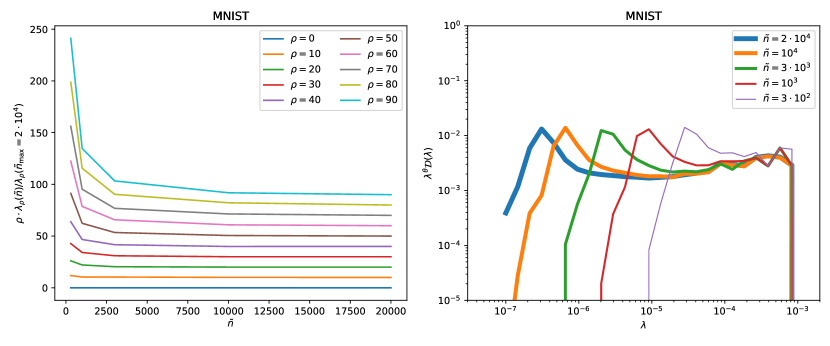
Refer to caption
Refer to caption
Figure 9: Left: we plot the first eigenvalues λρsubscript𝜆𝜌\lambda_{\rho} of Gram matrices of size n~~𝑛\tilde{n}, rescaled by the corresponding eigenvalue of the largest Gram matrix (top row is MNIST, bottom row is CIFAR10). Increasing n~~𝑛\tilde{n} the eigenvalues are expected to converge, and indeed these ratios asymptote to one. We are plotting one eigenvalue every 10 for the first 100 eigenvalues. In order to make the plot clearer we have multiplied each curve by a factor ρ𝜌\rho, equal to the eigenvalue index. Right: Density of eigenvalues of the Gram matrix, for several sizes n~~𝑛\tilde{n}, for MNIST (top) and CIFAR10 (bottom). The density is divided by the predicted asymptotic behavior (λρS)θsuperscriptsuperscriptsubscript𝜆𝜌𝑆𝜃\left(\lambda_{\rho}^{S}\right)^{-\theta}, with θ=1+αdeff𝜃1𝛼subscript𝑑eff\theta=1+\frac{\alpha}{d_{\mathrm{eff}}}. For a Laplace kernel αS=deff+1subscript𝛼𝑆subscript𝑑eff1\alpha_{S}=d_{\mathrm{eff}}+1 and for the effective dimension we used the values extracted in Section 7, resulting in θ1.937𝜃1.937\theta\approx 1.937 for MNIST and θ1.972𝜃1.972\theta\approx 1.972 for CIFAR10. This plot shows that the density of eigenvalues converges when n~~𝑛\tilde{n} increases, and that the predicted power law is consistent with observations.