11institutetext: Toyota Research Institute

An Unconditionally Stable First-Order
Constraint Solver for Multibody Systems

Evan M. Drumwright
Abstract

This article describes an absolutely stable, first-order constraint solver for multi-rigid body systems that calculates (predicts) constraint forces for typical bilateral and unilateral constraints, contact constraints with friction, and many other constraint types. Redundant constraints do not pose numerical problems or require regularization. Coulomb friction for contact is modeled using a true friction cone, rather than a linearized approximation. The computational expense of the solver is dependent upon the types of constraints present in the input. The hardest (in a computational complexity sense) inputs are reducible to solving convex optimization problems, i.e., polynomial time solvable. The simplest inputs require only solving a linear system. The solver is L-stable, which will imply that the forces due to constraints induce no computational stiffness into the multibody dynamics differential equations. This approach is targeted to multibodies simulated with coarse accuracy, subject to computational stiffness arising from constraints, and where the number of constraint equations is not large compared to the number of multibody position and velocity state variables. For such applications, the approach should prove far faster than using other implicit integration approaches. I assess the approach on some fundamental multibody dynamics problems.

1 Introduction

A constrained multi-body system is a collection of bodies subject to kinematic constraints, dynamic constraints, or both. Typical examples are robots, automobile suspensions, and containers of granules. The kinematics and dynamics of constrained multi-body systems can be formulated explicitly, by use of judiciously selected coordinates, or implicitly, through the use of constraint forces that must be computed to satisfy certain algebraic equations. Depending on the model and the input (state and any control inputs to the model), accounting for the effect of those constraints on the dynamics is often very expensive and potentially results in computational stiffness in the application (simulation, trajectory optimization, etc.) This article focuses on efficient solutions to initial value problems for multi-body systems subject to such implicit constraint equations, i.e., it focuses on simulating interesting multibody systems.

A constraint solver computes the aforementioned constraint forces (and through a simple linear operation, accelerations) acting on a multi-body system at a given state, under some modeling assumptions and using mathematical programming or nonlinear optimization algorithms (like solving complementarity problems). The notion of a constraint solver arises from the observation that the dynamics of a constrained multibody system is coupled to its constraint forces but these problems can actually be decoupled into those of (1) ​ computing the constraint forces via a constraint solver, i.e., solving an equation that looks like GM𝟣G𝖳λ=GM𝟣fG˙v𝐺superscript𝑀1superscript𝐺𝖳𝜆𝐺superscript𝑀1𝑓˙𝐺𝑣G{M}^{\mathsf{-1}}{G}^{\mathsf{T}}\lambda=-G{M}^{\mathsf{-1}}f-\dot{G}v for λ𝜆\lambda and (2) ​ computing the multibody accelerations by solving an equation that looks like Mv˙=G𝖳λ+f𝑀˙𝑣superscript𝐺𝖳𝜆𝑓M\dot{v}={G}^{\mathsf{T}}\lambda+f for v˙˙𝑣\dot{v}.

Constraint solvers are frequently used to help integrate multi-rigid body simulations with rigid constraints. They are used for modeling contact (and all other constraints) in engineering simulations, e.g., time-stepping based Algoryx and Vortex and event-based SimWise 4D. Constraint solvers have been applied to similar problems in control, state estimation, and system identification applications. Yet constraint solvers have suffered to date from problems both conceptual in the model (i.e., inconsistency and indeterminacy, inability to “invert” the model for optimizing control under constraints, non-smoothness of the model) and practical (i.e., constraint drift, difficulty of solving complementarity problems quickly and robustly).

This article introduces a constraint solver that calculates constraint forces under the realistic model that constraints are all at least minimally compliant (specifically, that they are no more stiff than representable using double precision floating point). Admitting some compliance, even a nominal amount, into the existing “hard” constraint formulations causes the aforementioned conceptual and practical challenges to disappear and the problem instances to become computationally easy to solve. And while computational stiffness has obstructed the use of very stiff constraints for simulation, I will show how the present approach is not susceptible to this problem, by design. As an additional bonus, the constraint solver is L-stable: any size integration step can be used to simulate a constrained system without the constraint forces giving rise to instability.

My constraint solver requires only one linear system solution or optimization per time interval; if optimization is required, the optimization problem is convex, even when modeling friction with a true cone, and the model does not require the discretization of the time interval to shrink for convergence. And, that single optimization is relatively inexpensive and robust, since finding a feasible point is trivially accomplished by setting some variables to “large” and the rest to zero. Sparsity in the problem is common and readily exploited. The constraint solver enjoys several other computational advantages. It does the minimum “collision detection” work (i.e., a single evaluation) per timestep and offers up to first-order accuracy. It is easy to construct smooth constraints for input to the model and thereby ensure that the constraint solver is differentiable. Finally, the computational implementation is straightforward.

1.1 Approach overview

Softening the “hard” constraints for multibody systems into compliant constraints (like those in the penalty model) cause the constraints to become dynamical systems. The constraints then couple motion to, and are influenced by, a multi-body system. One way to model the static and dynamic behavior of these compliant constraints is with multiple spring-dampers. Accordingly, I will describe a stable and efficient numerical approach that:

  1. 1.

    Given deformations ϕ(q)italic-ϕ𝑞\phi(q) and deformation rates ϕ˙(q,v)˙italic-ϕ𝑞𝑣\dot{\phi}(q,v) for the spring-dampers (i.e., the constraint system state variables) as functions of multibody state {q(t),v(t)}𝑞𝑡𝑣𝑡\{q(t),v(t)\} at time t𝑡t,

  2. 2.

    computes the spring-damper forces implicitly using future deformation and deformation rates (i.e., those at t+h𝑡t+h, for small hh),

  3. 3.

    and applies these computed spring-damper forces in a fast, explicit manner to integrate the multibody state to {q(t+h),v(t+h)}𝑞𝑡𝑣𝑡\{q(t+h),v(t+h)\}.

I will show how the implicit Euler approach is particularly efficient at integrating multi-spring-damper systems that are computationally stiff and potentially computationally stiff. I will also show how decoupling the multi-body and spring-mass systems, which makes their independent solution possible, still yields solutions with only second-order truncation error.

I will not describe how to model physical phenomena using the constraints. I assume that the user can define and evaluate spring-damper type constraint functions. But I will also demonstrate how various kinds of constraints can be modeled: joint constraints, range-of-motion limit constraints, and contact constraints—using both Hertzian contact and elastic foundation models—with Coulomb friction.

1.2 Focus application: multi-body simulation

This article will focus on the application of the constraint solver to the simulation problem: compute q(t+h)𝑞𝑡q(t+h), v(t+h)𝑣𝑡v(t+h) and constraint forces λ(t)𝜆𝑡\lambda(t) given q(t)𝑞𝑡q(t), v(t)𝑣𝑡v(t), and hh. These data are a superset of the necessary data for control, state estimation, and system identification purposes. Control applications, for instance, might require only computing λ(t)𝜆𝑡\lambda(t) if q(t+h)𝑞𝑡q(t+h) and v(t+h)𝑣𝑡v(t+h) may be obtained to high accuracy from sensor measurements. In any case, efficient application of the constraint solver to simulation implies efficient application to the control, state estimation, and system identification domains as well. We will see throughout this article that simulations using the constraint solver are most efficient—compared to other simulation approaches, like applying implicit integrators to the normally stiff differential equations arising from constraints—when the number of constraints is not large compared to the number of multibody position and velocity state variables. §5 will show a pathological counterexample (900 constraints vs. 13 state variables), in which the best-case performance of the constraint solver was not as good as optimized rivals, but its worst-case performance was far better than theirs.

1.3 Outline

The layout of this article follows. Section 2 surveys related work in modeling and solving constraints and the use of these models in control, state estimation, system identification, and simulation applications. Section 3 examines the spring-mass-damper system, which is the foundational model for the present work, and considers various first-order approaches for integrating the system dynamics. Section 4 uses the stable first-order approach examined in Section 3 to integrate the dynamics of a multi-rigid body system constrained using only bilateral constraints. Section 5 extends this approach to a unilaterally constrained system (e.g., a robot hitting a range-of-motion limit). Section 6 extends the approach yet again, this time to contact constraints with friction. Section 7 closes with concluding thoughts.

2 Related work

This section surveys two existing kinds of constraint solvers: ones that model constraint forces as a function of deformation (“penalty methods”, §2.1) and ones that compute forces to satisfy kinematic and force constraints (§2.2). §2.3 additionally surveys applications of constraint solvers to control, state estimation, system identification, and simulation domains.

2.1 Penalty methods

There is a vast literature covering compliant contact models, which are sometimes known as penalty methods. In the context of compliant contact models, deformation results in a proportional force. In the context of optimization via penalty methods, deformation can be viewed as the violation of a constraint, and solving the resulting DAE by treating it as an ODE with virtual penalization forces is effected using a kind of dynamic optimization. These virtual forces cause the constraint violations to be minimized dynamically (over time) in the absence of loads; in other words, the behavior of the system as it is stabilizing can be viewed analogously to the penalty method class of optimization algorithm. Summarizing, there are two very different approaches that both effect compliant contact. And the constraint solver introduced in this article draws from both approaches by modeling contact from first principles and by leveraging constrained optimization.

The contact aspects of the constraint model introduced in this article are effectively that of the Song et al. [20] contact model, though I introduce numerous computational and modeling advantages over the approach they describe. Mine does not require categorizing contact into sticking and sliding. My approach permits using realistic stiffness values derived via engineering tables and without needing to consider whether the choice of modeling parameters might make the simulation unstable.

2.2 Rigid constraints and rigid contact

Approaches that compute forces to satisfy kinematic constraints and force constraints have traditionally been applied to modeling rigid constraints. Perfectly rigid constraints often simplify multi-rigid body models in several respects, all of which are conferred through coordinate reduction: revolute and prismatic joints, to name but two examples, use interpretable, computationally efficient, and kinematically simple independent parameters. But the concept of rigid constraints can introduce some theoretical and practical challenges as well. As just one example, constraint forces can be distributed arbitrarily if care is not taken when constraints are both rigid and redundant; Zapolsky and Drumwright had to work around this particular problem in the design of a constraint-aware inverse dynamics controller for quadrupedal robots [26]. The constraint solver introduced in this article is also able to model bilateral constraints, and it allows them to be “rigid” up to full floating point precision; put another way, constraints can be modeled as rigid to a greater extent than is observed in nature. For example, the Young’s Modulus of diamond is on the order of a terapascal, which only requires twelve of the approximately sixteen decimal digits of precision provided by 64-bit floating point numbers, assuming that the pascal is the chosen unit.

A “rigid [point] contact”, i.e., a point of contact between two completely rigid bodies, corresponds to a unilateral rigid constraint and several more equations that describe the frictional interaction at that point (see, e.g., [24]). Rigid contact makes reasoning about the contact geometry simple, but the problems from redundant forces described above (also called “indeterminacy”) remain. The conceptual problem of “inconsistent configurations”, like Painlevé’s famous paradox (described in detail in [21]) emerges with rigid contact also. And rigid contact is non-smooth: force is discontinuous when two bodies first contact, for example. In addition to these challenges that arise from the mathematics (and likely the real physics as well, see, e.g. [3]), the computational demands of implementing such models are significant.

Specifically, it is challenging along multiple dimensions to solve the complementarity problems that emerge from the rigid contact formulations. Solutions are known to be non-unique.111The effect of that non-uniqueness on multi-body dynamics software is unknown, and that lack of knowledge is troubling given the potentially large number of software implementations using this approach for engineering purposes. Existence proofs only exist for problem approximations (i.e., discretization of the continuous time dynamics, polygonal friction cones). Even for the approximate problems that are known to possess solutions ([22, 2]) that can be found with an algorithm (i.e., solving linear complementarity problems with Lemke’s Algorithm), the worst-case time complexity is exponential. Additionally, the necessary algorithms do not lend themselves to robust numerical implementations: it is hard to guarantee solutions to tight accuracy (satisfying the non-negativity and complementarity conditions to tight tolerances), particularly when the complementarity problems become “degenerate” from redundancy in the constraints (see, e.g., [4], p. 340). Without accuracy guarantees, it is challenging for the solver to even identify when it has solved the problem.

In addition to these theoretical and practical challenges, implementation introduces several more wrinkles: (1) ​ Coulomb friction requires selecting a typically arbitrary tolerance for distinguishing between sliding and rolling/not-sliding. (2) ​ The rigid contact model requires distinguishing between impacting and sustained contact (using another arbitrary tolerance); the former mode requires applying an appropriate multi-body impacting constraint model (all constraints, including contact constraints with friction, range of motion constraints, etc., are potentially active during an impact, so an impact model that accounts for all of these is necessary). (3) ​ Considerable thought is necessary to identify the minimum “states” (as in the sense of a finite state machine; these kinds of states are typically called “modes”) for a multi-point rigid constraint model, and the logic to switch between the various modes is incredibly complex. I’m unaware of a peer-reviewed description of the necessary logic in existing literature.

Drumwright and Shell [5] and Todorov [23] both described modified rigid contact models toward alleviating these challenges. Unfortunately, neither model was capable of producing solutions consistent with non-impacting (i.e., “sustained”) contact mechanics, which requires complementarity. As already noted, the model described in this article is based on an established compliant model of contact that has not been controversial. Still, my approach allows the model to be effectively rigid, i.e., rigid to the 16 decimal digits that IEEE 754 double precision allows, but without any of the aforementioned computational headaches. Additionally, this newly introduced approach is easier to solve than the models from [5, 23], both of which require solving a positive semi-definite (PSD) linear complementarity problem (or, equivalently, a PSD quadratic program) to compute an initial feasible point.

2.3 Applications of constraint solvers

Constraint solvers have been applied in multiple domains, namely control, state estimation, system identification, and simulation. This section surveys applications of constraint solvers in these areas. Note that a constraint solver need not exist as an explicit code module; the constraint solver for a simulation with compliant contact can be considered to be the combination of the contact model and the ODE initial value problem solver (i.e., the integrator).

2.3.1 Constraint solvers for control

Constraint solvers for control have been investigated heavily in the context of robotics under the name “whole body control”. The basic formula has been to control a robot subject to contact constraints; other kinds of constraints can usually be incorporated into these formulations, but contact has been the traditional focus. Representative works include those of Todorov [23], Escande et al. [6], Feng et al. [8], and Zapolsky and Drumwright [25]. Rigid contact and Coulomb friction models are typically used, implying either a differential algebraic equation or a differential complementarity problem mathematical model that is a function of control inputs u𝑢u, e.g.:

x˙˙𝑥\displaystyle\dot{x} =f(x,u)absent𝑓𝑥𝑢\displaystyle=f(x,u) (1)
00\displaystyle 0 =g(x)absent𝑔𝑥\displaystyle=g(x) (2)

Inverting this model—computing u𝑢u given x𝑥x and x˙˙𝑥\dot{x}—is computationally expensive when f(.)f(.) and g(.)g(.) incorporate contact constraints. The inverse is not required to be unique [25].

The presented constraint solver does not require regularization (cf. [23]), does not assume rigidity (cf. [6, Kuindersma:2015, 8]), can use a true friction cone (cf. [25]), is always solvable (i.e., inconsistent constraints are not of concern) with a unique solution, and does not violate physical laws (cf. [23]).

2.3.2 Constraint solvers for state estimation

Estimating state (position and velocity) of contacting rigid bodies has been investigated in works by Zhang et al. [27], Pollard et al. [19], Kuindersma et al. [Kuindersma:2015], and Kumar et al. [15]. The promise is to use contact mechanics (or a gross approximation thereof) to compensate for the poor observability of object state while objects are being manipulated. Estimating state for contacting bodies has proven to be a particularly difficult problem, and the deficiencies in prior process models is just one of the challenges to be overcome [14]; Koval et al. note “particle starvation” as one such significant challenge [14]. However, it is clear that better (faster, more accurate) process models would be beneficial to state estimation; Zhang et al.’s complementarity-problem-based state estimator was shown to be too slow for real-time, even when applied to a robotic hand modeled with only three point contacts.

2.3.3 Constraint solvers for system identification

System identification is the process of estimating parameters for a plant (i.e., the “process model” or “transition model” in the context of state estimation) from telemetry data. Constraint solvers can be employed in the system identification process to estimate parameters of the contact model in particular (see, e.g., [7] where impact restitution is estimated and [13, 7] where the friction coefficient is estimated). The presented constraint solver provides smooth gradients that are useful for the optimization process used for system identification.

2.3.4 Constraint solvers for simulation

Constraint solvers for simulation exhibit particular challenges not present in the aforementioned domains. Compliant models tend to lead to computational stiffness, which limits simulation step sizes for reasons of stability rather than accuracy. Simulations with rigid contact constraints either use an event-driven scheme or are only zeroth-order accurate (i.e., the “velocity stepping” approaches), and simulations using rigid contact models tend to generate many events. Commercial software products have spanned all three of the approaches I described above: MSC’s Adams is known to use a compliant model, SimWise 4D is known to use an event-driven scheme with a rigid contact model, and Havok is known to use the zeroth-order rigid contact approach.

2.4 Summary

We have now seen how constraint solvers can be used in control, state estimation, system identification, and simulation applications, and we have examined the dichotomy of constraint solvers: “soft” (compliant) and “hard” (rigid). We will next examine the simple mass-spring-system that serves as the physical model of our soft constraints.

3 The Spring-Mass-Damper system

The foundational model of all constraints in this article is that of the mass-spring-damper system:

mx¨+bx˙+kx=f.𝑚¨𝑥𝑏˙𝑥𝑘𝑥𝑓\displaystyle m\ddot{x}+b\dot{x}+kx=f. (3)

Various types of forces can be modeled by using either the dynamics of this system or through the equivalent relationship:

λ=kxbx˙.𝜆𝑘𝑥𝑏˙𝑥\displaystyle\lambda=-kx-b\dot{x}. (4)

As just one example, the mass-spring-damper readily emulates linearly elastic contact, an oft reasonable model.

The following subsections will investigate how to integrate multibody systems that are subject to such constraints (i.e., have forces applied from such a forcing model) under a parameter range of k𝑘k that would correspond to springs constructed from various materials. As examples, longitudinal forces acting on a steel beam with cross-sectional area 1m21superscriptm21\ \textrm{m}^{2} and 111 m length would exhibit a stiffness (k𝑘k in N/m) equivalent to the Young’s Modulus of steel (1012absentsuperscript1012\approx 10^{12} Pa). The same beam made from stiff rubber might have a Young’s Modulus of 105superscript10510^{5} Pa. So, k𝑘k must be able to take on a rather large range. Setting damping/dissipation values in a principled way from material properties is an open problem: damping/dissipation is currently used to achieve a qualitative effect, even in accuracy-critical FEM codes. But it seems reasonable to require that the viscous damping parameter lies in the range b[0Nsm,1012Nsm]𝑏0Nsmsuperscript1012Nsmb\in[0\frac{\textrm{N}\cdot\textrm{s}}{\textrm{m}},10^{12}\frac{\textrm{N}\cdot\textrm{s}}{\textrm{m}}].

We next examine how various first-order schemes integrate this spring-mass-damper system forward in time. If a particular integration scheme is incapable of simulating the spring-mass-damper system under the targeted parameters with reasonably large step sizes, that same integrator will be unable to simulate a multi-body system subject to dynamic constraints with similar stiffnesses.

3.1 Stable first-order integration of a spring-mass-damper system

The canonical first-order formulation of the mass-spring-damper system is:

v𝑣\displaystyle v =x˙absent˙𝑥\displaystyle=\dot{x} (5)
v˙˙𝑣\displaystyle\dot{v} =fbvkxm.absent𝑓𝑏𝑣𝑘𝑥𝑚\displaystyle=\frac{f-bv-kx}{m}. (6)

The various Euler integration schemes simply represent various ways to discretize x(t1)𝑥subscript𝑡1x(t_{1}) and v(t1)𝑣subscript𝑡1v(t_{1}) to a first-order approximation of the continuous time dynamics around x(t0)𝑥subscript𝑡0x(t_{0}) and v(t0)𝑣subscript𝑡0v(t_{0}), where t1=t0+hsubscript𝑡1subscript𝑡0t_{1}=t_{0}+h. For shorthand, we’ll write x0subscript𝑥0x_{0}, v0subscript𝑣0v_{0}, etc. to refer to a particular state variable at a particular point in time.

3.1.1 Explicit Euler

The explicit Euler update rule takes the following form:

x1subscript𝑥1\displaystyle x_{1} =x0+hv0absentsubscript𝑥0subscript𝑣0\displaystyle=x_{0}+hv_{0} (7)
v1subscript𝑣1\displaystyle v_{1} =v0+hm(fbv0kx0),absentsubscript𝑣0𝑚𝑓𝑏subscript𝑣0𝑘subscript𝑥0\displaystyle=v_{0}+\frac{h}{m}(f-bv_{0}-kx_{0}), (8)

meaning that for f=0𝑓0f=0 the problem can be treated as a linear difference equation:

y1subscript𝑦1\displaystyle y_{1} =Ay0,absent𝐴subscript𝑦0\displaystyle=Ay_{0}, (9)

where y[xv]𝖳𝑦superscriptmatrix𝑥𝑣𝖳y\equiv{\begin{bmatrix}x&v\end{bmatrix}}^{\mathsf{T}} and the iteration matrix is defined as:

A[1hhkm 1hbm].𝐴matrix1𝑘𝑚1𝑏𝑚\displaystyle A\equiv\begin{bmatrix}1&h\\ \frac{-hk}{m}&\ 1-\frac{hb}{m}\end{bmatrix}. (10)

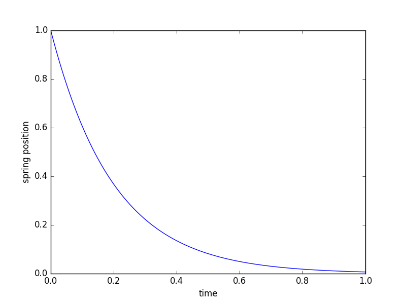
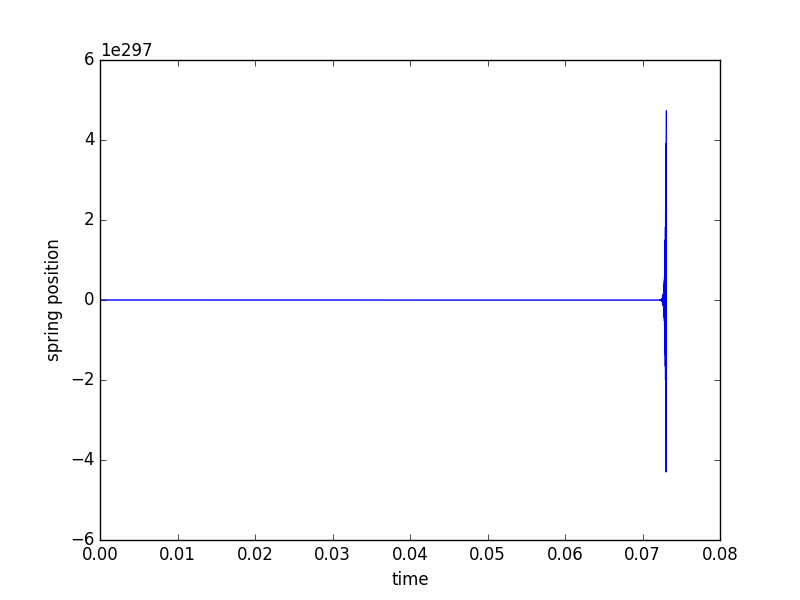
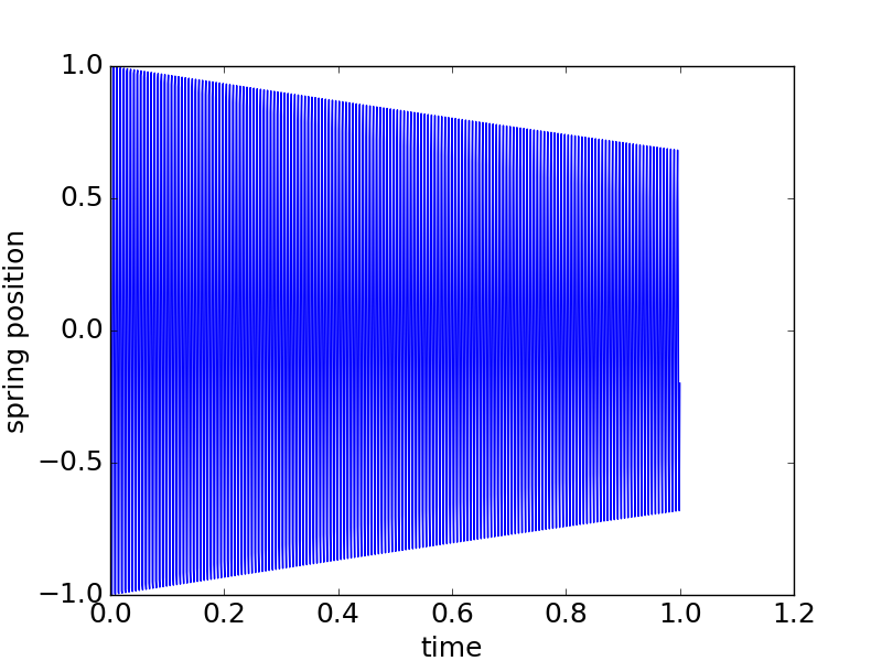
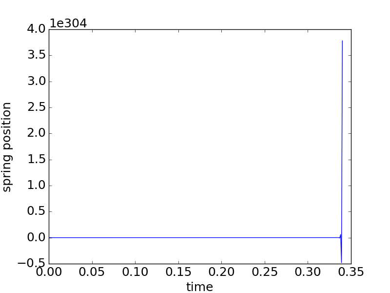
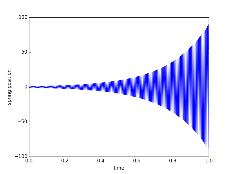
The iteration matrix’s eigenvalues shows that the approach is not stable for any step size (for stability, the magnitudes of all eigenvalues, real and imaginary, must be less than unity). Figure 1 shows that explicit Euler is clearly unstable for h=105,k=106,b=1formulae-sequencesuperscript105formulae-sequence𝑘superscript106𝑏1h=10^{-5},k=10^{6},b=1, somewhat more stable for h=105,k=106,b=10formulae-sequencesuperscript105formulae-sequence𝑘superscript106𝑏10h=10^{-5},k=10^{6},b=10, stable for h=105,k=106,b=2×10⁵formulae-sequencesuperscript105formulae-sequence𝑘superscript106𝑏2superscript105h=10^{-5},k=10^{6},b=2\times 10^{5}, and unstable for h=105,k=106,b=2.1×10⁵formulae-sequencesuperscript105formulae-sequence𝑘superscript106𝑏2.1superscript105h=10^{-5},k=10^{6},b=2.1\times 10^{5}. For the range of parameters we wish to use for k𝑘k and b𝑏b, explicit Euler is clearly unsuitable.
Refer to caption
Refer to caption
Refer to caption
Figure 1: Explicit Euler integration of a spring-mass-damper system with f=0,h=105formulae-sequence𝑓0superscript105f=0,h=10^{-5}, m=1𝑚1m=1, k=106𝑘superscript106k=10^{6} for b=1𝑏1b=1 (top), b=2×10⁵𝑏2superscript105b=2\times 10^{5} (middle), and b=2.1×10⁵𝑏2.1superscript105b=2.1\times 10^{5} (bottom). Explicit Euler is not stable under the targeted range of conditions.

3.1.2 Semi-implicit Euler

From [10] (1.9), the following update rule yields the semi-implicit Euler integrator, which is symplectic:

x1subscript𝑥1\displaystyle x_{1} =x0+hv1absentsubscript𝑥0subscript𝑣1\displaystyle=x_{0}+hv_{1} (11)
v1subscript𝑣1\displaystyle v_{1} =v0+hm(fbv1kx0).absentsubscript𝑣0𝑚𝑓𝑏subscript𝑣1𝑘subscript𝑥0\displaystyle=v_{0}+\frac{h}{m}(f-bv_{1}-kx_{0}). (12)

Symplectic integrators have been applied to problems extensively for their momentum conserving properties. However, while semi-implicit Euler is stable for any non-negative value of b𝑏b, it is not stable for any non-negative k𝑘k, as Figure 2 shows.

Refer to caption
Refer to caption
Figure 2: Semi-implicit Euler integration of a spring-mass-damper system with f=0,h=103formulae-sequence𝑓0superscript103f=0,h=10^{-3} , m=1𝑚1m=1, and b=1𝑏1b=1 for k=106𝑘superscript106k=10^{6} (left) and k=107𝑘superscript107k=10^{7} (right). Semi-implicit Euler is only stable when k𝑘k is sufficiently small.

3.1.3 Implicit Euler

The implicit Euler update rule

x1subscript𝑥1\displaystyle x_{1} =x0+hv1absentsubscript𝑥0subscript𝑣1\displaystyle=x_{0}+hv_{1} (13)
v1subscript𝑣1\displaystyle v_{1} =v0+hm(fbv1kx1)absentsubscript𝑣0𝑚𝑓𝑏subscript𝑣1𝑘subscript𝑥1\displaystyle=v_{0}+\frac{h}{m}(f-bv_{1}-kx_{1}) (14)

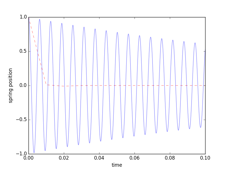
is well known to be stable for any step size, and Figure 3 illustrates this behavior. This integration scheme typically introduces significant computational requirements for arbitrary systems, however, as determining the next states typically requires solving nonlinear systems of equations. The next section will show how the approach introduced in this article is able to avoid this computationally hard problem.
Refer to caption
Figure 3: Implicit integration of the mass-spring system with f=0,k=106formulae-sequence𝑓0𝑘superscript106f=0,k=10^{6}, m=1𝑚1m=1, and b=0𝑏0b=0 for h=105superscript105h=10^{-5} (blue) and h=102superscript102h=10^{-2} (red, dashed). The integration is stable for any step size, though it is clear that the solutions are not particularly accurate—the amplitude should not attenuate.

3.2 Conclusion

For integrating mass-spring-damper systems with k𝑘k and b𝑏b in our target range, a stiff integration technique is necessary. But implicit integrators may be avoided in multibody dynamics simulations because the requisite nonlinear equation solutions can prove prohibitively expensive (especially when bodies are contacting). The artificial dissipation introduced by implicit methods (illustrated in Figure 3) is often a lesser concern.

4 Application of the solution of the mass-spring-damper system to multibody systems with holonomic constraints

The last section showed that a stiff integration (implicit) technique permits stable integration of mass-spring-damper systems with the necessary parameter ranges. This section will introduce a new DAE formulation for multibody systems subject to spring-damper forcing models (or, equivalently, subject to kinematic constraints) and will show how to integrate this system (i.e., solve initial value problems for the DAE formulation) by building on the implicit Euler algorithm described in the previous section.

Consider a multi-body system having m𝑚m generalized coordinates q(t)𝑞𝑡q(t) which are constrained by n𝑛n holonomic functions ϕi(t,q)subscriptitalic-ϕ𝑖𝑡𝑞\phi_{i}(t,q), for i{1,,n}𝑖1𝑛i\in\{1,\ldots,n\} (the subscript will only be called out when necessary hereafter). The usual way that this constraint is modeled is as “hard” in the sense that solutions are sought that satisfy ϕ(t,q)=0italic-ϕ𝑡𝑞0\phi(t,q)=0 to high accuracy (generally somewhat less than full double precision). Without loss of generality, I will ignore the version of the constraint that is an explicit function of time, i.e., ϕ(q)=0italic-ϕ𝑞0\phi(q)=0. Now imagine that the constraint is no longer to be modeled as hard, where its “violation” should be zero, but instead acts as a virtual spring and damper that produces a force λ𝜆\lambda that penalizes deviation from rest:

λ=Kϕ(q)Bϕ˙(q,v)M^G˙v,𝜆𝐾italic-ϕ𝑞𝐵˙italic-ϕ𝑞𝑣^𝑀˙𝐺𝑣\displaystyle\lambda=-K\phi(q)-B\dot{\phi}(q,v)-\hat{M}\dot{G}v, (15)

for some choice of non-negative diagonal matrices Bn×n𝐵superscript𝑛𝑛B\in\mathbb{R}^{n\times n} and Kn×n𝐾superscript𝑛𝑛K\in\mathbb{R}^{n\times n}, and where the variables G𝐺G (and, by extension, its time derivative) and M^^𝑀\hat{M} will be defined shortly. This viewpoint of a constraint could be useful for simulating a four bar linkage by virtually welding two rigid bodies together. Or, we might wish to model a contact patch between two bodies using springs with stiffnesses K𝐾K and damping B𝐵B. In fact, this equation is very close to how penalty methods are applied in multi-body simulation, in which initial value problems for the following ordinary differential equation are solved:

q˙˙𝑞\displaystyle\dot{q} =Nvabsent𝑁𝑣\displaystyle=Nv (16)
Mv˙𝑀˙𝑣\displaystyle M\dot{v} =G𝖳λ+f(t,q,v)absentsuperscript𝐺𝖳𝜆𝑓𝑡𝑞𝑣\displaystyle={G}^{\mathsf{T}}\lambda+f(t,q,v) (17)
λ𝜆\displaystyle\lambda =Kϕ(q)Bϕ˙(q,v),absent𝐾italic-ϕ𝑞𝐵˙italic-ϕ𝑞𝑣\displaystyle=-K\phi(q)-B\dot{\phi}(q,v), (18)

where v(t)𝑣𝑡v(t) are now the system generalized velocities, M(q)𝑀𝑞M(q) is the generalized inertia matrix, f(t,q,v)𝑓𝑡𝑞𝑣f(t,q,v) is every force but constraint forces acting on the multi-body system, N(q)𝑁𝑞N(q) is a left-invertible matrix that maps elements in v𝑣v to elements in q˙˙𝑞\dot{q}, and G(q)=ϕqN𝐺𝑞italic-ϕ𝑞𝑁G(q)=\frac{\partial\phi}{\partial q}N. This latter variable comes from taking the time-derivative of ϕ(q):ϕ˙=ϕqq˙:italic-ϕ𝑞˙italic-ϕitalic-ϕ𝑞˙𝑞\phi(q):\dot{\phi}=\frac{\partial\phi}{\partial q}\dot{q} and using exactly the relationship we just described, q˙=Nv˙𝑞𝑁𝑣\dot{q}=Nv. G𝐺G also yields linear mappings from generalized velocities to constraint velocities and (through transposition) constraint forces to generalized forces.222This duality arises from mechanical power, which relates velocity and force. The astute reader will note that the M^G˙v^𝑀˙𝐺𝑣\hat{M}\dot{G}v term from (15) is absent in (18). I’m showing how forces are applied in the context of the penalty method in (15), and I will shortly provide reasoning for the inclusion of the mysterious M^G˙v^𝑀˙𝐺𝑣\hat{M}\dot{G}v term.

4.1 Explicitly coupling the multibody and spring-damper systems

The system of ODEs above does not explicitly consider the dynamics of the constraint (i.e., its trajectory over time), but we will by requiring that it acts as a mass-spring-damper system:

M^ϕ¨(q,v,v˙)+Bϕ˙(q,v)+Kϕ(q)=f^.^𝑀¨italic-ϕ𝑞𝑣˙𝑣𝐵˙italic-ϕ𝑞𝑣𝐾italic-ϕ𝑞^𝑓\displaystyle\hat{M}\ddot{\phi}(q,v,\dot{v})+B\dot{\phi}(q,v)+K\phi(q)=\hat{f}. (19)

where M^^𝑀\hat{M} is a particular kind of inertia (I call it the “constraint-space inertia matrix”) and f^^𝑓\hat{f} is a force in constraint space. This system has a single fixed point at {ϕ(q)=0,ϕ˙(q,v)=0}formulae-sequenceitalic-ϕ𝑞0˙italic-ϕ𝑞𝑣0\{\phi(q)=0,\dot{\phi}(q,v)=0\}. I will show that the following DAE, which combines the system of ODEs above with (19), permits computing efficient solutions to initial value problems for q(t)𝑞𝑡q(t) and v(t)𝑣𝑡v(t):

q˙˙𝑞\displaystyle\dot{q} =Nvabsent𝑁𝑣\displaystyle=Nv (20)
Mv˙𝑀˙𝑣\displaystyle M\dot{v} =G𝖳λ+f(t,q,v)absentsuperscript𝐺𝖳𝜆𝑓𝑡𝑞𝑣\displaystyle={G}^{\mathsf{T}}\lambda+f(t,q,v) (21)
00\displaystyle 0 =g(t,q,v,v˙)=M^ϕ¨(q,v,v˙)+B(q,v)ϕ˙(q,v)+K(q)ϕ(q)f^absent𝑔𝑡𝑞𝑣˙𝑣^𝑀¨italic-ϕ𝑞𝑣˙𝑣𝐵𝑞𝑣˙italic-ϕ𝑞𝑣𝐾𝑞italic-ϕ𝑞^𝑓\displaystyle=g(t,q,v,\dot{v})=\hat{M}\ddot{\phi}(q,v,\dot{v})+B(q,v)\dot{\phi}(q,v)+K(q)\phi(q)-\hat{f} (22)
λ𝜆\displaystyle\lambda =K(q)ϕ(q)B(q,v)ϕ˙(q,v)M^G˙v,absent𝐾𝑞italic-ϕ𝑞𝐵𝑞𝑣˙italic-ϕ𝑞𝑣^𝑀˙𝐺𝑣\displaystyle=-K(q)\phi(q)-B(q,v)\dot{\phi}(q,v)-\hat{M}\dot{G}v, (23)

where:

M^^𝑀\displaystyle\hat{M} (GM𝟣G𝖳)𝟣absentsuperscript𝐺superscript𝑀1superscript𝐺𝖳1\displaystyle\equiv{(G{M}^{\mathsf{-1}}{G}^{\mathsf{T}})}^{\mathsf{-1}} (24)
f^^𝑓\displaystyle\hat{f} M^GM𝟣f.absent^𝑀𝐺superscript𝑀1𝑓\displaystyle\equiv\hat{M}G{M}^{\mathsf{-1}}f. (25)

Note that K𝐾K and B𝐵B have been “promoted” from constant terms (in the penalty method) to state-dependent terms, allowing, e.g., stiffnesses to be configuration dependent (which is necessary for correctly modeling linear elasticity) and contact forces to be smooth (by making B𝐵B a function of ϕ(q)italic-ϕ𝑞\phi(q) as in [12], thereby eliminating a possible discontinuity around ϕ=0italic-ϕ0\phi=0). I will demonstrate how K𝐾K and B𝐵B can be computed using proper units in different applications (range-of-motion limits, elastic foundation contact, non-conforming contact) in examples examined throughout this article.

Why this DAE? It explicitly declares the coupled dynamical systems: the multibody system and the spring-mass-damper system. The spring-mass-damper system is expressed in a form where the parameters (K𝐾K and B𝐵B) are easily interpretable and its behavior readily analyzed. As just two simple examples, we could identify the undamped oscillation frequency or damping ratio.

Now let us examine the DAE applied to a particle, with mass m𝑚m and state (x,x˙)formulae-sequence𝑥˙𝑥(x\in\mathbb{R},\dot{x}\in\mathbb{R}), that is compliantly constrained to the environment using a virtual mass-spring-damper: M^ϕ¨+Bϕ˙+Kϕ=f^^𝑀¨italic-ϕ𝐵˙italic-ϕ𝐾italic-ϕ^𝑓\hat{M}\ddot{\phi}+B\dot{\phi}+K\phi=\hat{f}. Consider how the system of ODEs in (20)–(23) is simplified when m𝑚m\in\mathbb{R} replaces M𝑀M, 111 (unity) replaces N𝑁N, x𝑥x replaces q𝑞q, x˙˙𝑥\dot{x} replaces v𝑣v, and ϕ(x)xitalic-ϕ𝑥𝑥\phi(x)\equiv x:

mx¨=𝑚¨𝑥absent\displaystyle m\ddot{x}= f+λ𝑓𝜆\displaystyle f+\lambda (26)
f^=^𝑓absent\displaystyle\hat{f}= M^ϕ¨+Bϕ˙+Kϕ^𝑀¨italic-ϕ𝐵˙italic-ϕ𝐾italic-ϕ\displaystyle\hat{M}\ddot{\phi}+B\dot{\phi}+K\phi (27)
λ=𝜆absent\displaystyle\lambda= KϕBϕ˙.𝐾italic-ϕ𝐵˙italic-ϕ\displaystyle-K\phi-B\dot{\phi}. (28)

Since ϕ/q=G=1italic-ϕ𝑞𝐺1\partial\phi/\partial q=G=1, we have replaced G𝖳λsuperscript𝐺𝖳𝜆{G}^{\mathsf{T}}\lambda in (21) with just λ𝜆\lambda and M^G˙v^𝑀˙𝐺𝑣\hat{M}\dot{G}v with zero in (23). From ϕ(x)xitalic-ϕ𝑥𝑥\phi(x)\equiv x we can obtain ϕ˙=x˙˙italic-ϕ˙𝑥\dot{\phi}=\dot{x} and ϕ¨=x¨¨italic-ϕ¨𝑥\ddot{\phi}=\ddot{x}. It should now be apparent that the particle is equivalent to a spring-mass-damper with stiffness K𝐾K and damper B𝐵B that is affixed to the environment when M^=m^𝑀𝑚\hat{M}=m and f^=f^𝑓𝑓\hat{f}=f.

Similarly, we can attach a rigid body system to the environment using springs and dampers and seek the same effect (with respect to stiffness, damping, and inertia). To bridge the ODE for ϕitalic-ϕ\phi (Equation 22) with the ODEs for q𝑞q and v𝑣v (Equations 20 and 21), we use the observation ϕ˙=ϕqq˙=ϕqNv˙italic-ϕitalic-ϕ𝑞˙𝑞italic-ϕ𝑞𝑁𝑣\dot{\phi}=\frac{\partial\phi}{\partial q}\dot{q}=\frac{\partial\phi}{\partial q}Nv to define GϕqN𝐺italic-ϕ𝑞𝑁G\equiv\frac{\partial\phi}{\partial q}N, implying ϕ˙=Gv˙italic-ϕ𝐺𝑣\dot{\phi}=Gv (it can be shown that G𝐺G is the transpose of the force transmission matrix) and:

ϕ¨=Gv˙+G˙v,¨italic-ϕ𝐺˙𝑣˙𝐺𝑣\displaystyle\ddot{\phi}=G\dot{v}+\dot{G}v, (29)

as well. Rearranging (21):

v˙=M𝟣(G𝖳λ+f),˙𝑣superscript𝑀1superscript𝐺𝖳𝜆𝑓\displaystyle\dot{v}={M}^{\mathsf{-1}}({G}^{\mathsf{T}}\lambda+f), (30)

we can substitute v˙˙𝑣\dot{v} into (29), yielding:

ϕ¨=GM𝟣G𝖳λ+GM𝟣f+G˙v.¨italic-ϕ𝐺superscript𝑀1superscript𝐺𝖳𝜆𝐺superscript𝑀1𝑓˙𝐺𝑣\displaystyle\ddot{\phi}=G{M}^{\mathsf{-1}}{G}^{\mathsf{T}}\lambda+G{M}^{\mathsf{-1}}f+\dot{G}v. (31)

We now substitute the definition of λ𝜆\lambda from (23):

ϕ¨=GM𝟣G𝖳(Bϕ˙KϕG˙v)+GM𝟣f+G˙v.¨italic-ϕ𝐺superscript𝑀1superscript𝐺𝖳𝐵˙italic-ϕ𝐾italic-ϕ˙𝐺𝑣𝐺superscript𝑀1𝑓˙𝐺𝑣\displaystyle\ddot{\phi}=G{M}^{\mathsf{-1}}{G}^{\mathsf{T}}(-B\dot{\phi}-K\phi-\dot{G}v)+G{M}^{\mathsf{-1}}f+\dot{G}v. (32)

Moving all ϕitalic-ϕ\phi terms and derivatives to the left hand side:

ϕ¨+GM𝟣G𝖳(Bϕ˙+KϕM^G˙v)=GM𝟣f+G˙v,¨italic-ϕ𝐺superscript𝑀1superscript𝐺𝖳𝐵˙italic-ϕ𝐾italic-ϕ^𝑀˙𝐺𝑣𝐺superscript𝑀1𝑓˙𝐺𝑣\displaystyle\ddot{\phi}+G{M}^{\mathsf{-1}}{G}^{\mathsf{T}}(B\dot{\phi}+K\phi-\hat{M}\dot{G}v)=G{M}^{\mathsf{-1}}f+\dot{G}v, (33)

and noting that we want the equation to look like (22), we multiply both sides by M^^𝑀\hat{M} to arrive at:

M^ϕ¨+M^GM𝟣G𝖳(Bϕ˙+Kϕ+M^G˙v)=M^GM𝟣f+M^G˙v.^𝑀¨italic-ϕ^𝑀𝐺superscript𝑀1superscript𝐺𝖳𝐵˙italic-ϕ𝐾italic-ϕ^𝑀˙𝐺𝑣^𝑀𝐺superscript𝑀1𝑓^𝑀˙𝐺𝑣\displaystyle\hat{M}\ddot{\phi}+\hat{M}G{M}^{\mathsf{-1}}{G}^{\mathsf{T}}(B\dot{\phi}+K\phi+\hat{M}\dot{G}v)=\hat{M}G{M}^{\mathsf{-1}}f+\hat{M}\dot{G}v. (34)

Using the prior definitions M^=(GM𝟣G𝖳)𝟣^𝑀superscript𝐺superscript𝑀1superscript𝐺𝖳1\hat{M}={(G{M}^{\mathsf{-1}}{G}^{\mathsf{T}})}^{\mathsf{-1}} and f^=M^GM𝟣f^𝑓^𝑀𝐺superscript𝑀1𝑓\hat{f}=\hat{M}G{M}^{\mathsf{-1}}f, we can simplify this to:

M^ϕ¨+Bϕ˙+Kϕ=f^.^𝑀¨italic-ϕ𝐵˙italic-ϕ𝐾italic-ϕ^𝑓\displaystyle\hat{M}\ddot{\phi}+B\dot{\phi}+K\phi=\hat{f}. (35)

In other words, the rigid body system acts like a mass-spring-system affixed to the environment given λ𝜆\lambda as defined in (23). Also note that (22) is redundant in the DAE: it follows from the definitions of λ𝜆\lambda, M^^𝑀\hat{M}, and f^^𝑓\hat{f} as shown above.

I will now show that it is possible to compute the evolution of the constraint dynamics independently of q1subscript𝑞1q_{1} and v1subscript𝑣1v_{1} with a first-order solution. This will allow me to show that a solution method can leverage the computationally easy problem of implicitly advancing the state of a spring-damper system with the also easy problem of explicitly (or semi-explicitly) advancing the state of a multi-rigid body system, all while remaining (at least) first-order accurate. The upshot is that the method is efficient and stable whatever the magnitudes of K𝐾K and B𝐵B.

4.2 First-order scheme: formulating multibody constraint problems with purely bilateral constraints

The challenge with applying an ODE initial value problem solver (i.e., integrator) to (20)–(23) directly is that the equations are prone to introducing computational stiffness (when K𝐾K or B𝐵B) is large. The method of choice for computationally stiff ODEs is an implicit integrator, as we observed in Section 3, but implicit integrators are usually inefficient when the equations aren’t stiff; explicit integrators are the method of choice in that case. The solution to this efficiency problem would seem to be a scheme that can switch between the two approaches (implicit and explicit) as appropriate. Such automatic stiffness detection has rarely proven to be efficient in practice (see [11], pp. 21–24).

Instead, I will now describe a particular first-order scheme for the previous constrained multibody system, including the necessary sequence of operations. This particular scheme was constructed to have particular qualities. First, the ODEs for the constraint variables are solved implicitly (for stability). Second, the ODEs for q𝑞q and v𝑣v, i.e., (20) and (21), are solved semi-explicitly (v𝑣v is computed explicitly, then that value is used to compute q𝑞q), which avoids solving nonlinear systems of equations and minimizes creep for sticking friction (when friction is introduced into the model, in Section 6). The scheme follows.

Given q0subscript𝑞0q_{0}, v0subscript𝑣0v_{0}, N0subscript𝑁0N_{0}, M0subscript𝑀0M_{0}, G0subscript𝐺0G_{0}, f(q0,v0)𝑓subscript𝑞0subscript𝑣0f(q_{0},v_{0}), ϕ0subscriptitalic-ϕ0\phi_{0}, and ϕ˙0subscript˙italic-ϕ0\dot{\phi}_{0}, compute:

q1subscript𝑞1\displaystyle q_{1} =q0+hN0v1+O(h2)absentsubscript𝑞0subscript𝑁0subscript𝑣1𝑂superscript2\displaystyle=q_{0}+hN_{0}v_{1}+O(h^{2}) (36)
v1subscript𝑣1\displaystyle v_{1} =v0+hM01(G0𝖳λ1+f0)+O(h2)absentsubscript𝑣0superscriptsubscript𝑀01superscriptsubscript𝐺0𝖳subscript𝜆1subscript𝑓0𝑂superscript2\displaystyle=v_{0}+hM_{0}^{-1}({G_{0}}^{\mathsf{T}}\lambda_{1}+f_{0})+O(h^{2}) (37)
ϕ1subscriptitalic-ϕ1\displaystyle\phi_{1} =ϕ0+hϕ˙1+O(h2)absentsubscriptitalic-ϕ0subscript˙italic-ϕ1𝑂superscript2\displaystyle=\phi_{0}+h\dot{\phi}_{1}+O(h^{2}) (38)
ϕ˙1subscript˙italic-ϕ1\displaystyle\dot{\phi}_{1} =ϕ˙0+hϕ¨0+O(h2).absentsubscript˙italic-ϕ0subscript¨italic-ϕ0𝑂superscript2\displaystyle=\dot{\phi}_{0}+h\ddot{\phi}_{0}+O(h^{2}). (39)

As this section has moved the discussion from the realm of algebra to numerical implementation, further consideration of the 0 and 1 notation is necessary. Subscript-00 denotes a quantity to be evaluated as an input to the problem. On the other hand, subscript-111 denotes a variable to be solved for; these variables are what the constraint solver computes. We want to have as few subscript-111 variables as possible, and those variables should not be “buried” within a function; consider that e.g., (36) specified instead as q1=q0+hN1v1+O(h2)subscript𝑞1subscript𝑞0subscript𝑁1subscript𝑣1𝑂superscript2q_{1}=q_{0}+hN_{1}v_{1}+O(h^{2}) would require solving a nonlinear system of equations for q1subscript𝑞1q_{1} (which we will avoid since many collision detection calls would be necessary in evaluating N1subscript𝑁1N_{1}). Finally, variables not specified with a subscript will not be evaluated; these variables will be used solely to simplify complicated expressions.

My accuracy analysis will make use of the following two lemmas.

Lemma 1

A function of a time-dependent vector (e.g., f(x(t))𝑓𝑥𝑡f(x(t))) that can be well approximated by a Taylor Series around x(t)𝑥𝑡x(t) can be approximated with linear error without consideration of any Jacobian terms.

Proof

The proof is evident using only the first two terms of the Taylor Series expansion:

f(x(t+h))=f(x(t))+hfxx˙+O(h2).𝑓𝑥𝑡𝑓𝑥𝑡𝑓𝑥˙𝑥𝑂superscript2\displaystyle f(x(t+h))=f(x(t))+h\frac{\partial f}{\partial x}\dot{x}+O(h^{2}). (40)

And therefore

f(x(t+h))=f(x(t))+O(h).𝑓𝑥𝑡𝑓𝑥𝑡𝑂\displaystyle f(x(t+h))=f(x(t))+O(h). (41)
Lemma 2

Any time-dependent term in an ODE evaluated at time t0subscript𝑡0t_{0} that is approximated by its value at t0+hsubscript𝑡0t_{0}+h introduces O(h2)𝑂superscript2O(h^{2}) truncation error into the solution of the initial value problem at t0+hsubscript𝑡0t_{0}+h.

Proof

Consider the first two terms in the Taylor Series, f(x(t0+h))=f(x(t0))+hf˙(x(t0),x˙(t0))+O(h2)𝑓𝑥subscript𝑡0𝑓𝑥subscript𝑡0˙𝑓𝑥subscript𝑡0˙𝑥subscript𝑡0𝑂superscript2f(x(t_{0}+h))=f(x(t_{0}))+h\dot{f}(x(t_{0}),\dot{x}(t_{0}))+O(h^{2}); this is equivalent to  (40) because f˙=fxx˙˙𝑓𝑓𝑥˙𝑥\dot{f}=\frac{\partial f}{\partial x}\dot{x}. Evaluating x(t0)𝑥subscript𝑡0x(t_{0}), to pick one term arbitrarily, at t0+hsubscript𝑡0t_{0}+h instead of t0subscript𝑡0t_{0} introduces an error of O(h)𝑂O(h) into f˙˙𝑓\dot{f}’s evaluation, from Lemma 1:

f(x(t0+h))=𝑓𝑥subscript𝑡0absent\displaystyle f(x(t_{0}+h))= f(x(t))|x(t0)+h(f˙(x(t),x˙(t))|x(t0+h),x˙(t0)+O(h))+evaluated-at𝑓𝑥𝑡𝑥subscript𝑡0evaluated-at˙𝑓𝑥𝑡˙𝑥𝑡𝑥subscript𝑡0˙𝑥subscript𝑡0𝑂\displaystyle f(x(t))|_{x(t_{0})}+h(\dot{f}(x(t),\dot{x}(t))|_{x(t_{0}+h),\dot{x}(t_{0})}+O(h))+\ldots (42)
O(h2).𝑂superscript2\displaystyle\quad O(h^{2}).

The hO(h)=O(h2)𝑂𝑂superscript2hO(h)=O(h^{2}) term is subsumed by the existing O(h2)𝑂superscript2O(h^{2}) term. It should be clear that any combination of substitutions of x(t)𝑥𝑡x(t) and x˙(t)˙𝑥𝑡\dot{x}(t) by their values at x(t+h)𝑥𝑡x(t+h) and x˙(t+h)˙𝑥𝑡\dot{x}(t+h), respectively, results in identical truncation error.

Theorem 1

Integrating ϕ(q)italic-ϕ𝑞\phi(q) and ϕ˙(q,v)˙italic-ϕ𝑞𝑣\dot{\phi}(q,v) independently from q𝑞q and v𝑣v, all from initial time t0subscript𝑡0t_{0}, yields solutions at t1subscript𝑡1t_{1} for ϕ(q1)italic-ϕsubscript𝑞1\phi(q_{1}), ϕ˙(q1,v1)˙italic-ϕsubscript𝑞1subscript𝑣1\dot{\phi}(q_{1},v_{1}), that exhibit quadratic truncation error in h=t1t0subscript𝑡1subscript𝑡0h=t_{1}-t_{0}.

Proof

The proof will start from the explicit Euler algorithm applied to ϕitalic-ϕ\phi and ϕ˙˙italic-ϕ\dot{\phi}. Explicit Euler is known to be locally first-order accurate (equivalent to saying that the truncation error is quadratic). Quadratic truncation error will be maintained through every step. Explicit Euler applied to ϕitalic-ϕ\phi and ϕ˙˙italic-ϕ\dot{\phi} yields the equations:

ϕ1subscriptitalic-ϕ1\displaystyle\phi_{1} =ϕ0+hϕ˙0+O(h2)absentsubscriptitalic-ϕ0subscript˙italic-ϕ0𝑂superscript2\displaystyle=\phi_{0}+h\dot{\phi}_{0}+O(h^{2}) (43)
ϕ˙1subscript˙italic-ϕ1\displaystyle\dot{\phi}_{1} =ϕ˙0+hϕ¨0+O(h2).absentsubscript˙italic-ϕ0subscript¨italic-ϕ0𝑂superscript2\displaystyle=\dot{\phi}_{0}+h\ddot{\phi}_{0}+O(h^{2}). (44)

This approach can be transformed into a semi-explicit Euler method by using the identity ϕ˙0=ϕ˙1+O(h)subscript˙italic-ϕ0subscript˙italic-ϕ1𝑂\dot{\phi}_{0}=\dot{\phi}_{1}+O(h) and applying Lemma 2 to (43):

ϕ1subscriptitalic-ϕ1\displaystyle\phi_{1} =ϕ0+hϕ˙1+O(h2)absentsubscriptitalic-ϕ0subscript˙italic-ϕ1𝑂superscript2\displaystyle=\phi_{0}+h\dot{\phi}_{1}+O(h^{2}) (45)

Thus, (45) and (44) represent the foundation of the integration scheme. We now demarcate evaluation times for the “bridging equation”, (29):

ϕ¨0=G0v˙0+G˙0v0,subscript¨italic-ϕ0subscript𝐺0subscript˙𝑣0subscript˙𝐺0subscript𝑣0\displaystyle\ddot{\phi}_{0}=G_{0}\dot{v}_{0}+\dot{G}_{0}v_{0}, (46)

and for (21) as well, rearranging slightly first:

v˙0=M0𝟣(G0𝖳λ0+f0).subscript˙𝑣0superscriptsubscript𝑀01superscriptsubscript𝐺0𝖳subscript𝜆0subscript𝑓0\displaystyle\dot{v}_{0}={M_{0}}^{\mathsf{-1}}({G_{0}}^{\mathsf{T}}\lambda_{0}+f_{0}). (47)

Applying Lemma 1 to this equation allows us to establish the relationship:

v˙0=M0𝟣(G0𝖳λ1+f0)+O(h).subscript˙𝑣0subscriptsuperscript𝑀10superscriptsubscript𝐺0𝖳subscript𝜆1subscript𝑓0𝑂\displaystyle\dot{v}_{0}={M}^{\mathsf{-1}}_{0}({G_{0}}^{\mathsf{T}}\lambda_{1}+f_{0})+O(h). (48)

Then substituting (48) into (46) yields:

ϕ¨0subscript¨italic-ϕ0\displaystyle\ddot{\phi}_{0} =G0(M0𝟣(G0𝖳λ1+f0)+O(h))v˙0+G˙0v0.absentsubscript𝐺0subscriptsuperscriptsubscript𝑀01superscriptsubscript𝐺0𝖳subscript𝜆1subscript𝑓0𝑂subscript˙𝑣0subscript˙𝐺0subscript𝑣0\displaystyle=G_{0}\underbrace{\big{(}{M_{0}}^{\mathsf{-1}}({G_{0}}^{\mathsf{T}}\lambda_{1}+f_{0})+O(h)\big{)}}_{\dot{v}_{0}}+\dot{G}_{0}v_{0}. (49)

And substituting that into (44) gives:

ϕ˙1subscript˙italic-ϕ1\displaystyle\dot{\phi}_{1} =ϕ˙0+h(G0(M0𝟣(G0𝖳λ1+f0))+G˙0v0)ϕ0¨+O(h2),\displaystyle=\dot{\phi}_{0}+h(\underbrace{G_{0}({M_{0}}^{\mathsf{-1}}({G_{0}}^{\mathsf{T}}\lambda_{1}+f_{0}))+\dot{G}_{0}v_{0})}_{\ddot{\phi_{0}}}+O(h^{2}), (50)

from Lemma 2.

Combining (38) and (50) and an additional equation for λ1subscript𝜆1\lambda_{1} (Equation 23 with specified times for K𝐾K, B𝐵B, ϕitalic-ϕ\phi and ϕ˙˙italic-ϕ\dot{\phi}) yields three blocks of equations in three blocks of unknowns (ϕ1subscriptitalic-ϕ1\phi_{1}, ϕ˙1subscript˙italic-ϕ1\dot{\phi}_{1}, and λ1subscript𝜆1\lambda_{1}):

ϕ1subscriptitalic-ϕ1\displaystyle\phi_{1} =ϕ0+hϕ˙1+O(h2)absentsubscriptitalic-ϕ0subscript˙italic-ϕ1𝑂superscript2\displaystyle=\phi_{0}+h\dot{\phi}_{1}+O(h^{2}) (51)
ϕ˙1subscript˙italic-ϕ1\displaystyle\dot{\phi}_{1} =ϕ˙0+h(G0(M0𝟣(G0𝖳λ1+f0))+G˙0v0)+O(h2)absentsubscript˙italic-ϕ0subscript𝐺0superscriptsubscript𝑀01superscriptsubscript𝐺0𝖳subscript𝜆1subscript𝑓0subscript˙𝐺0subscript𝑣0𝑂superscript2\displaystyle=\dot{\phi}_{0}+h\big{(}G_{0}({M_{0}}^{\mathsf{-1}}({G_{0}}^{\mathsf{T}}\lambda_{1}+f_{0}))+\dot{G}_{0}v_{0}\big{)}+O(h^{2}) (52)
λ1subscript𝜆1\displaystyle\lambda_{1} =K0ϕ1B0ϕ˙1(G0M0𝟣G0𝖳)𝟣G˙0v0+O(h).absentsubscript𝐾0subscriptitalic-ϕ1subscript𝐵0subscript˙italic-ϕ1superscriptsubscript𝐺0subscriptsuperscript𝑀10subscriptsuperscript𝐺𝖳01subscript˙𝐺0subscript𝑣0𝑂\displaystyle=-K_{0}\phi_{1}-B_{0}\dot{\phi}_{1}-{(G_{0}{M}^{\mathsf{-1}}_{0}{G}^{\mathsf{T}}_{0})}^{\mathsf{-1}}\dot{G}_{0}v_{0}+O(h). (53)

Note the provenance of the O(h)𝑂O(h) term for the last equation comes from mixing evaluation times, in accordance with Lemma 1. We can solve the 3 block ×\times 3 block linear system above by first substituting (53) into (52), yielding:

ϕ˙1subscript˙italic-ϕ1\displaystyle\dot{\phi}_{1} =ϕ˙0+absentsubscript˙italic-ϕ0\displaystyle=\dot{\phi}_{0}+\ldots (54)
h(G0(M0𝟣(G0𝖳(K0ϕ1B0ϕ˙1(G0M0𝟣G0𝖳)𝟣G˙0v0+O(h))λ1+\displaystyle\quad h\big{(}G_{0}({M_{0}}^{\mathsf{-1}}({G_{0}}^{\mathsf{T}}\underbrace{(-K_{0}\phi_{1}-B_{0}\dot{\phi}_{1}-{(G_{0}{M}^{\mathsf{-1}}_{0}{G}^{\mathsf{T}}_{0})}^{\mathsf{-1}}\dot{G}_{0}v_{0}+O(h))}_{\lambda_{1}}+\ldots
f0))+G˙0v0)+O(h2)\displaystyle\qquad f_{0}))+\dot{G}_{0}v_{0}\big{)}+O(h^{2})

G0M0𝟣G0𝖳(G0M0𝟣G0𝖳)𝟣subscript𝐺0subscriptsuperscript𝑀10subscriptsuperscript𝐺𝖳0superscriptsubscript𝐺0subscriptsuperscript𝑀10subscriptsuperscript𝐺𝖳01G_{0}{M}^{\mathsf{-1}}_{0}{G}^{\mathsf{T}}_{0}{(G_{0}{M}^{\mathsf{-1}}_{0}{G}^{\mathsf{T}}_{0})}^{\mathsf{-1}} yields the identity matrix, leaving us with hG˙0v0subscript˙𝐺0subscript𝑣0-h\dot{G}_{0}v_{0} and hG˙0v0subscript˙𝐺0subscript𝑣0h\dot{G}_{0}v_{0} terms, which cancel. Also, the hO(h)𝑂hO(h) term is subsumed by the O(h2)𝑂superscript2O(h^{2}) term, allowing us to remove it. Combining both simplifications, we arrive at:

ϕ˙1subscript˙italic-ϕ1\displaystyle\dot{\phi}_{1} =ϕ˙0+h(G0(M0𝟣(G0𝖳(K0ϕ1B0ϕ˙1+f0)))+O(h2).\displaystyle=\dot{\phi}_{0}+h\big{(}G_{0}({M_{0}}^{\mathsf{-1}}({G_{0}}^{\mathsf{T}}(-K_{0}\phi_{1}-B_{0}\dot{\phi}_{1}+f_{0}))\big{)}+O(h^{2}). (55)

We next substitute (51) into this equation, yielding:

ϕ˙1subscript˙italic-ϕ1\displaystyle\dot{\phi}_{1} =ϕ˙0+h(G0(M0𝟣(G0𝖳(K0(ϕ0+hϕ˙1+O(h2))ϕ1B0ϕ˙1)+f0))+O(h2).\displaystyle=\dot{\phi}_{0}+h\big{(}G_{0}({M_{0}}^{\mathsf{-1}}({G_{0}}^{\mathsf{T}}(-K_{0}\underbrace{(\phi_{0}+h\dot{\phi}_{1}+O(h^{2}))}_{\phi_{1}}-B_{0}\dot{\phi}_{1})+f_{0}))+O(h^{2}). (56)

Now the hO(h2)𝑂superscript2hO(h^{2}) term is subsumed by the O(h2)𝑂superscript2O(h^{2}) term:

ϕ˙1subscript˙italic-ϕ1\displaystyle\dot{\phi}_{1} =ϕ˙0+h(G0(M0𝟣(G0𝖳(K0(ϕ0+hϕ˙1)B0ϕ˙1)+f0))+)+O(h2).absentsubscript˙italic-ϕ0limit-fromsubscript𝐺0superscriptsubscript𝑀01superscriptsubscript𝐺0𝖳subscript𝐾0subscriptitalic-ϕ0subscript˙italic-ϕ1subscript𝐵0subscript˙italic-ϕ1subscript𝑓0𝑂superscript2\displaystyle=\dot{\phi}_{0}+h\big{(}G_{0}({M_{0}}^{\mathsf{-1}}({G_{0}}^{\mathsf{T}}(-K_{0}(\phi_{0}+h\dot{\phi}_{1})-B_{0}\dot{\phi}_{1})+f_{0}))+\big{)}+O(h^{2}). (57)

When we move all ϕ˙1subscript˙italic-ϕ1\dot{\phi}_{1} terms to the left hand side, we arrive at:

(I+h(G0(M0𝟣(G0𝖳(hK0+B0))))ϕ˙1=ϕ˙0+\displaystyle(I+h\big{(}G_{0}({M_{0}}^{\mathsf{-1}}({G_{0}}^{\mathsf{T}}(hK_{0}+B_{0})))\big{)}\dot{\phi}_{1}=\dot{\phi}_{0}+\ldots (58)
h(G0(M0𝟣(G0𝖳(K0ϕ0+f0)))+O(h2).\displaystyle\qquad h\big{(}G_{0}({M_{0}}^{\mathsf{-1}}({G_{0}}^{\mathsf{T}}(-K_{0}\phi_{0}+f_{0}))\big{)}+O(h^{2}).

Collecting terms and simplifying using the following definitions:

M^0subscript^𝑀0\displaystyle\hat{M}_{0} (G0M0𝟣G0𝖳)𝟣absentsuperscriptsubscript𝐺0superscriptsubscript𝑀01superscriptsubscript𝐺0𝖳1\displaystyle\equiv{(G_{0}{M_{0}}^{\mathsf{-1}}{G_{0}}^{\mathsf{T}})}^{\mathsf{-1}} (59)
Y𝑌\displaystyle Y (I+M^0𝟣(h2K0+hB0))𝟣,absentsuperscript𝐼superscriptsubscript^𝑀01superscript2subscript𝐾0subscript𝐵01\displaystyle\equiv{(I+{\hat{M}_{0}}^{\mathsf{-1}}(h^{2}K_{0}+hB_{0}))}^{\mathsf{-1}}, (60)

we obtain:

ϕ˙1subscript˙italic-ϕ1\displaystyle\dot{\phi}_{1} =Y(ϕ˙0hM^0𝟣K0ϕ0+hG0M0𝟣f0)+O(h2)absent𝑌subscript˙italic-ϕ0superscriptsubscript^𝑀01subscript𝐾0subscriptitalic-ϕ0subscript𝐺0superscriptsubscript𝑀01subscript𝑓0𝑂superscript2\displaystyle=Y(\dot{\phi}_{0}-h{\hat{M}_{0}}^{\mathsf{-1}}K_{0}\phi_{0}+hG_{0}{M_{0}}^{\mathsf{-1}}f_{0})+O(h^{2}) (61) ϕ1subscriptitalic-ϕ1\displaystyle\phi_{1} =ϕ0+hϕ˙1+O(h2).absentsubscriptitalic-ϕ0subscript˙italic-ϕ1𝑂superscript2\displaystyle=\phi_{0}+h\dot{\phi}_{1}+O(h^{2}). (62)

The computation of λ1subscript𝜆1\lambda_{1} (via Equation 53) permits evaluating v1subscript𝑣1v_{1} (via Equation 37), which in turn permits evaluating q1subscript𝑞1q_{1} (via Equation 36). No step of the scheme has given up beyond quadratic truncation error for the state variables (q𝑞q, v𝑣v, ϕitalic-ϕ\phi, and ϕ˙˙italic-ϕ\dot{\phi}). Therefore, (61) and (62) yield first-order accurate solutions ϕ(q1)italic-ϕsubscript𝑞1\phi(q_{1}) and ϕ˙(q1,v1)˙italic-ϕsubscript𝑞1subscript𝑣1\dot{\phi}(q_{1},v_{1}) without accurate knowledge of the value of q1subscript𝑞1q_{1} and v1subscript𝑣1v_{1}. \blacksquare


For the remainder of this article, I will continue to assume that f𝑓f and B𝐵B are evaluated using q0,v0subscript𝑞0subscript𝑣0q_{0},v_{0} and N𝑁N, G𝐺G, M𝑀M and K𝐾K are evaluated using q0subscript𝑞0q_{0}, allowing us to drop the subscripts used previously. Thus ff0𝑓subscript𝑓0f\equiv f_{0}, NN0𝑁subscript𝑁0N\equiv N_{0}, GG0𝐺subscript𝐺0G\equiv G_{0}, G˙G˙0˙𝐺subscript˙𝐺0\dot{G}\equiv\dot{G}_{0}, KK0𝐾subscript𝐾0K\equiv K_{0}, BB0𝐵subscript𝐵0B\equiv B_{0}, MM0𝑀subscript𝑀0M\equiv M_{0}, f^f^0^𝑓subscript^𝑓0\hat{f}\equiv\hat{f}_{0} and M^M^0^𝑀subscript^𝑀0\hat{M}\equiv\hat{M}_{0}.


4.3 Implications

Conceptually, the first-order scheme described in the previous subsection provides an algorithm for integrating two coupled sets of dynamical systems—the multibody system and the constraints—independently and with first-order accuracy.

This result is profound: it means that stiff, or even rigid, holonomic constraint forces can be computed efficiently using only the solution to a linear system. No nonlinear system of equations needs to be solved, which also means that step sizes do not need to be limited to ensure convergence of a Newton-Raphson scheme (cf. [11], pp. 123–126). The resulting constraint forces can then be used with at least any first-order integration scheme; extension to higher order schemes might also be possible.

Also note that the matrix Y𝑌Y is always invertible. It is the sum of a positive definite matrix (I𝐼I, the identity matrix) and the product of a positive semi-definite matrix and a linear combination of positive semi-definite, diagonal matrices (K𝐾K and B𝐵B). Given that u𝖳Iu>0superscript𝑢𝖳𝐼𝑢0{u}^{\mathsf{T}}Iu>0 and u𝖳(h(hK+B))u0superscript𝑢𝖳𝐾𝐵𝑢0{u}^{\mathsf{T}}(h(hK+B))u\geq 0, Y𝑌Y must be positive definite as well, because

u𝖳(I+h(hK+B))u>0superscript𝑢𝖳𝐼𝐾𝐵𝑢0\displaystyle{u}^{\mathsf{T}}(I+h(hK+B))u>0 (63)

for any vector u𝑢u of nonzero real values. Positive definite matrices are always invertible (in fact, their inverses are positive definite as well). The implication of the invertibility of Y𝑌Y is that constraint forces become distributed among the constraints: indeterminacy is resolved organically. The approaches for unilateral and contact constraints will share this nice property also.

Finally we address the question of how such stability is attained for so little computational cost. The key is that the forces due to the constraints do not cause computational stiffness; it is still possible to introduce computational forces through other forces (e.g., large PD control terms) applied to the multibody system. Instead, the constraint-based approach removes any computational stiffness from the constraints.

4.4 Example: pendulum

The constraint-based approach was used to simulate a pendulum in 2D using an absolute coordinate formulation. The configuration of the bob was represented using three-coordinates: center-of-mass location (two coordinates, x𝑥x and y𝑦y) and bob orientation (one coordinate, θ𝜃\theta). The velocity variables were simply x˙,y˙˙𝑥˙𝑦\dot{x},\dot{y}, and θ˙˙𝜃\dot{\theta}. The holonomic constraint was:

ϕ=[xy]+R(θ)u,italic-ϕmatrix𝑥𝑦𝑅𝜃𝑢\displaystyle\phi=\begin{bmatrix}x\\ y\end{bmatrix}+R(\theta)u, (64)

where R(θ)𝑅𝜃R(\theta) is an orientation matrix that transforms vectors in the bob’s body frame to the world frame and u𝑢u is a vector from the bob to the nominal joint location. The pendulum was started in the fully horizontal position with zero velocity and was simulated for one second of virtual time. At every time step, (61) and (62) were used to determine the next ϕ˙˙italic-ϕ\dot{\phi} and ϕitalic-ϕ\phi, respectively, which were used in turn to compute, via (53), λ1subscript𝜆1\lambda_{1}. λ1subscript𝜆1\lambda_{1} was used in turn to compute the next q𝑞q and v𝑣v (via the symplectic scheme represented by Equations 37 and 36).

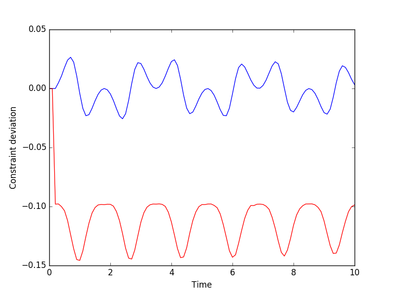
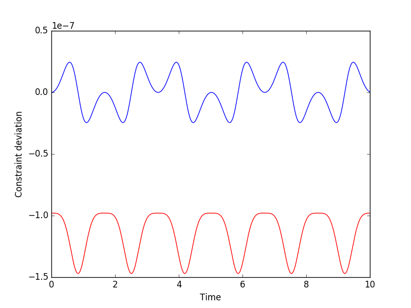
Figure 4 shows the constraint deviation under large stiffnesses for both a large (h=0.10.1h=0.1) and small (h=104superscript104h=10^{-4}) step sizes; note that these “errors” scale quadratically with hh, consistent with the O(h2)𝑂superscript2O(h^{2}) error proved in Section 4.2. The symplectic scheme caused the energy of the pendulum to be maintained to precisely zero. Observers who have experience with implicit integration techniques, which numerically effect some artificial dissipation, might be wondering how the scheme conserves energy for large step sizes. The explanation is that momentum orthogonal to the constraint is conserved. An example in the next section will show that system energy indeed dissipates whenever momentum is not orthogonal to the constraints.
Refer to caption
Refer to caption
Figure 4: Deviation of the pendulum from its nominal joint position under the parameters k=1015𝑘superscript1015k=10^{15} and b=1𝑏1b=1 for h=0.10.1h=0.1 (left) and h=104superscript104h=10^{-4} (right) . While the stiffness is large, the system does not become unstable. Note the different scales in the two plots.

5 Unilaterally constrained spring-damper model

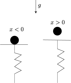
While bilateral constraints are useful to introduce the methodology underlying my approach, the hard technical challenges usually emerge in multibody dynamics only after unilateral constraints—and the complementarity problems used to model the dynamics—are introduced. And so I will now demonstrate how we can apply my approach to multibody systems subject to unilateral constraints. Consider the following system composed of a spring-damper affixed to the “world” that can compress arbitrarily but not extend past its resting length, and a particle that can move only along one dimension. When the particle enters the region x0𝑥0x\leq 0, the spring is considered to be compressed. The spring can only push (i.e., not pull) against the particle (i.e., only compressive forces are allowed). When the spring is at its resting length (implied by x>0𝑥0x>0), it can impart no force on the particle. Figure 5 depicts these conditions.
Refer to caption
Figure 5: An illustration of the unilateral spring system modeling contact between a particle with height x𝑥x and “the world”; we are interested in how the spring-damper system imparts forces on the particle. We assume that the spring can only compress; it cannot extend past its resting length. The surface of the spring-damper system can only impart forces on the particle when the spring is compressed (left); it is assumed both that the spring is at its resting length and that the rate of change of the resting length is zero when x>0𝑥0x>0 (right). The figure also shows the direction of gravity.

5.1 Holonomic unilateral constraint formulation for multibody systems

Consider the multibody system with state (q,v)𝑞𝑣(q,v), vector function of n𝑛n holonomic, unilateral constraint functions ϕ(q)nitalic-ϕ𝑞superscript𝑛\phi(q)\to\mathbb{R}^{n}, generalized inertia matrix M𝑀M, Jacobian matrix G = ϕqNitalic-ϕ𝑞𝑁\frac{\partial\phi}{\partial q}N, and external force vector f(q,v)𝑓𝑞𝑣f(q,v). Stiffness and damping scalars k𝑘k and b𝑏b again become non-negative diagonal matrices Kn×n𝐾superscript𝑛𝑛K\in\mathbb{R}^{n\times n} and Bn×n𝐵superscript𝑛𝑛B\in\mathbb{R}^{n\times n}.

I use a piecewise DAE model333A piecewise DAE is a sequence in time of (typically related) differential algebraic equations, where the initial conditions for the ithsuperscript𝑖thi^{\textrm{th}} DAE are drawn from the solution to the (i1)thsuperscript𝑖1th(i-1)^{\textrm{th}} DAE, and the initial conditions for the first DAE are specified by the user., where the “pieces” correspond to times where a constraint becomes active (i.e., where ϕitalic-ϕ\phi is non-positive and λ𝜆\lambda transitions from zero to positive) or inactive (i.e., where λ𝜆\lambda transitions from positive to zero). No better than first-order accuracy can be obtained without an event-detection mechanism that isolates times in which constraints transition from active to inactive and vice versa [1].

I will reformulate this DAE as a differential programming problem (DPP), which combines ordinary differential equations with mathematical programming variables, where solution to the latter is necessary to solve initial value problems over the former. The mathematical programming problem in my particular formulation is a convex quadratic program for which the solution (to λ𝜆\lambda) yields the maximum value of zero and Kϕ(q)Bϕ˙(q,v)M^G˙v𝐾italic-ϕ𝑞𝐵˙italic-ϕ𝑞𝑣^𝑀˙𝐺𝑣-K\phi(q)-B\dot{\phi}(q,v)-\hat{M}\dot{G}v, obviating an otherwise necessary discontinuous nonlinear equality constraint (namely λ=max(0,Kϕ(q)Bϕ˙(q,v)M^G˙v)𝜆0𝐾italic-ϕ𝑞𝐵˙italic-ϕ𝑞𝑣^𝑀˙𝐺𝑣\lambda=\max{(0,-K\phi(q)-B\dot{\phi}(q,v)-\hat{M}\dot{G}v)} for unknown λ,ϕ𝜆italic-ϕ\lambda,\phi, and ϕ˙˙italic-ϕ\dot{\phi}).

5.2 DAE model of a unilaterally constrained system

The version of the DAE from (20)–(23) modified to model a purely compressive, compliant unilateral constraint is given below:

q˙=˙𝑞absent\displaystyle\dot{q}= Nv𝑁𝑣\displaystyle\ Nv (65)
Mv˙=𝑀˙𝑣absent\displaystyle M\dot{v}= G𝖳λ+fsuperscript𝐺𝖳𝜆𝑓\displaystyle\ {G}^{\mathsf{T}}\lambda+f (66)
f^=^𝑓absent\displaystyle\hat{f}= M^ϕ¨+Bϕ˙+Kϕ^𝑀¨italic-ϕ𝐵˙italic-ϕ𝐾italic-ϕ\displaystyle\ \hat{M}\ddot{\phi}+B\dot{\phi}+K\phi (67)
λ=𝜆absent\displaystyle\lambda= max(0,KϕBϕ˙M^G˙v).0𝐾italic-ϕ𝐵˙italic-ϕ^𝑀˙𝐺𝑣\displaystyle\max{(0,-K\phi-B\dot{\phi}-\hat{M}\dot{G}v}). (68)

The nonlinear equality constraint in (68) makes this DAE very challenging to solve. Nonlinear systems of equations are challenging to solve in general, as feasible points can be hard to find and success is usually dependent upon having a good starting point. And (68) is not differentiable at λ=0𝜆0\lambda=0, stymieing typical derivative-based search strategies. However, the DAE above is equivalent to the following DPP that computes λ𝜆\lambda via a convex quadratic program:

minλsubscriptmin𝜆\displaystyle\operatorname*{min}_{\lambda} 12λ𝖳λ12superscript𝜆𝖳𝜆\displaystyle\frac{1}{2}{\lambda}^{\mathsf{T}}\lambda (69)
q˙=˙𝑞absent\displaystyle\dot{q}= Nv𝑁𝑣\displaystyle\ Nv
Mv˙=𝑀˙𝑣absent\displaystyle M\dot{v}= G𝖳λ+fsuperscript𝐺𝖳𝜆𝑓\displaystyle\ {G}^{\mathsf{T}}\lambda+f
f^=^𝑓absent\displaystyle\hat{f}= M^ϕ¨+Bϕ˙+Kϕ^𝑀¨italic-ϕ𝐵˙italic-ϕ𝐾italic-ϕ\displaystyle\ \hat{M}\ddot{\phi}+B\dot{\phi}+K\phi
λ𝜆absent\displaystyle\lambda\geq KϕBϕ˙M^G˙v𝐾italic-ϕ𝐵˙italic-ϕ^𝑀˙𝐺𝑣\displaystyle\ -K\phi-B\dot{\phi}-\hat{M}\dot{G}v (70)
λ𝜆absent\displaystyle\lambda\geq 0.0\displaystyle\ 0. (71)

where recall that we have defined:

M^^𝑀absent\displaystyle\hat{M}\equiv (GM𝟣G𝖳)𝟣superscript𝐺superscript𝑀1superscript𝐺𝖳1\displaystyle\ {(G{M}^{\mathsf{-1}}{G}^{\mathsf{T}})}^{\mathsf{-1}}
f^^𝑓absent\displaystyle\hat{f}\equiv M^GM𝟣f^𝑀𝐺superscript𝑀1𝑓\displaystyle\ \hat{M}G{M}^{\mathsf{-1}}f

in (24) and (25), respectively. Computing the minimum value of a number that is at least as large as two other numbers is simply a maximization operation. In contrast to the previous DAE that required solving a nonlinear system of equations, the quadratic program above is trivial to solve.

This particular DPP will also prove useful when I introduce contact constraints with friction. For now, we analyze the convexity and feasibility of this problem when it is used to solve the time-discretized version of this problem for {λ,ϕ1,ϕ˙1}𝜆subscriptitalic-ϕ1subscript˙italic-ϕ1\{\lambda,\phi_{1},\dot{\phi}_{1}\}.

5.3 The time-discretized DPP for a unilaterally constrained system

Discretizing in time, removing (67)—these dynamics follow from the definition of λ𝜆\lambda, so (67) is redundant—and ignoring v1subscript𝑣1v_{1} and q1subscript𝑞1q_{1} momentarily yields:

minλ1,ϕ1,ϕ˙1subscriptminsubscript𝜆1subscriptitalic-ϕ1subscript˙italic-ϕ1\displaystyle\operatorname*{min}_{\lambda_{1},\phi_{1},\dot{\phi}_{1}}\ 12λ1𝖳λ112superscriptsubscript𝜆1𝖳subscript𝜆1\displaystyle\frac{1}{2}{\lambda_{1}}^{\mathsf{T}}{\lambda_{1}} (72)
ϕ1subscriptitalic-ϕ1\displaystyle\phi_{1} =ϕ0+hϕ˙1+O(h2)absentsubscriptitalic-ϕ0subscript˙italic-ϕ1𝑂superscript2\displaystyle=\phi_{0}+h\dot{\phi}_{1}+O(h^{2}) (73)
ϕ˙1subscript˙italic-ϕ1\displaystyle\dot{\phi}_{1} =ϕ˙0+h(Gv˙0+G˙v0)ϕ0¨+O(h2)absentsubscript˙italic-ϕ0subscript𝐺subscript˙𝑣0˙𝐺subscript𝑣0¨subscriptitalic-ϕ0𝑂superscript2\displaystyle=\dot{\phi}_{0}+h\underbrace{(G\dot{v}_{0}+\dot{G}v_{0})}_{\ddot{\phi_{0}}}+O(h^{2}) (74)
λ1subscript𝜆1\displaystyle\lambda_{1} Kϕ1Bϕ˙1M^0G˙v+O(h)absent𝐾subscriptitalic-ϕ1𝐵subscript˙italic-ϕ1subscript^𝑀0˙𝐺𝑣𝑂\displaystyle\geq-K\phi_{1}-B\dot{\phi}_{1}-\hat{M}_{0}\dot{G}v+O(h) (75)
λ1subscript𝜆1\displaystyle\lambda_{1} 0,absent0\displaystyle\geq 0, (76)

where the O(h)𝑂O(h) term in (75) comes from Lemma 1, and we use (46) in (74). Simplifying (74) further, we obtain:

minλ1,ϕ1,ϕ˙1subscriptminsubscript𝜆1subscriptitalic-ϕ1subscript˙italic-ϕ1\displaystyle\operatorname*{min}_{\lambda_{1},\phi_{1},\dot{\phi}_{1}}\ 12λ1𝖳λ112superscriptsubscript𝜆1𝖳subscript𝜆1\displaystyle\frac{1}{2}{\lambda_{1}}^{\mathsf{T}}{\lambda_{1}}
ϕ1subscriptitalic-ϕ1\displaystyle\phi_{1} =ϕ0+hϕ˙1+O(h2)absentsubscriptitalic-ϕ0subscript˙italic-ϕ1𝑂superscript2\displaystyle=\phi_{0}+h\dot{\phi}_{1}+O(h^{2})
ϕ˙1subscript˙italic-ϕ1\displaystyle\dot{\phi}_{1} =ϕ˙0+h(GM𝟣(G𝖳λ1+f+O(h))v˙0+G˙v0)+O(h2)absentsubscript˙italic-ϕ0𝐺subscriptsuperscript𝑀1superscript𝐺𝖳subscript𝜆1𝑓𝑂subscript˙𝑣0˙𝐺subscript𝑣0𝑂superscript2\displaystyle=\dot{\phi}_{0}+h(G\underbrace{{M}^{\mathsf{-1}}({G}^{\mathsf{T}}\lambda_{1}+f+O(h))}_{\dot{v}_{0}}+\dot{G}v_{0})+O(h^{2}) (77)
λ1subscript𝜆1\displaystyle\lambda_{1} Kϕ1Bϕ˙1M^G˙v+O(h)absent𝐾subscriptitalic-ϕ1𝐵subscript˙italic-ϕ1^𝑀˙𝐺𝑣𝑂\displaystyle\geq-K\phi_{1}-B\dot{\phi}_{1}-\hat{M}\dot{G}v+O(h)
λ1subscript𝜆1\displaystyle\lambda_{1} 0,absent0\displaystyle\geq 0,

from (66), where the O(h)𝑂O(h) term again comes from Lemma 1. As before, that term is scaled by hh and thus becomes subsumed by the existing O(h2)𝑂superscript2O(h^{2}) term:

ϕ˙1subscript˙italic-ϕ1\displaystyle\dot{\phi}_{1} =ϕ˙0+h(GM𝟣(G𝖳λ1+f)+G˙v0)+O(h2).absentsubscript˙italic-ϕ0𝐺superscript𝑀1superscript𝐺𝖳subscript𝜆1𝑓˙𝐺subscript𝑣0𝑂superscript2\displaystyle=\dot{\phi}_{0}+h(G{M}^{\mathsf{-1}}({G}^{\mathsf{T}}\lambda_{1}+f)+\dot{G}v_{0})+O(h^{2}). (78)

The QP can be simplified by substituting out ϕ1subscriptitalic-ϕ1\phi_{1} and ϕ˙1subscript˙italic-ϕ1\dot{\phi}_{1} in (75). Starting with the former,

λ1subscript𝜆1\displaystyle\lambda_{1} K(ϕ0+hϕ˙1+O(h2))ϕ1Bϕ˙1M^G˙v0+O(h),absent𝐾subscriptsubscriptitalic-ϕ0subscript˙italic-ϕ1𝑂superscript2subscriptitalic-ϕ1𝐵subscript˙italic-ϕ1^𝑀˙𝐺subscript𝑣0𝑂\displaystyle\geq-K\underbrace{(\phi_{0}+h\dot{\phi}_{1}+O(h^{2}))}_{\phi_{1}}-B\dot{\phi}_{1}-\hat{M}\dot{G}v_{0}+O(h), (79)

and then collecting terms yields:

λ1subscript𝜆1\displaystyle\lambda_{1} Kϕ0(hK+B)ϕ˙1M^G˙v0+O(h).absent𝐾subscriptitalic-ϕ0𝐾𝐵subscript˙italic-ϕ1^𝑀˙𝐺subscript𝑣0𝑂\displaystyle\geq-K\phi_{0}-(hK+B)\dot{\phi}_{1}-\hat{M}\dot{G}v_{0}+O(h). (80)

Then, replacing ϕ˙1subscript˙italic-ϕ1\dot{\phi}_{1} results in

λ1subscript𝜆1\displaystyle\lambda_{1} Kϕ0(hK+B)(ϕ˙0+hM^𝟣λ+hGM𝟣f+hG˙v0+O(h2))ϕ˙1absent𝐾subscriptitalic-ϕ0𝐾𝐵subscriptsubscript˙italic-ϕ0superscript^𝑀1𝜆𝐺superscript𝑀1𝑓˙𝐺subscript𝑣0𝑂superscript2subscript˙italic-ϕ1\displaystyle\geq-K\phi_{0}-(hK+B)\underbrace{(\dot{\phi}_{0}+h{\hat{M}}^{\mathsf{-1}}\lambda+hG{M}^{\mathsf{-1}}f+h\dot{G}v_{0}+O(h^{2}))}_{\dot{\phi}_{1}}-\ldots
M^G˙v+O(h).^𝑀˙𝐺𝑣𝑂\displaystyle\qquad\hat{M}\dot{G}v+O(h). (81)

The result after collecting terms and removing the subsumed hO(h2)𝑂superscript2hO(h^{2}) term is:

(I+(h2K+hB)M^𝟣)λ1𝐼superscript2𝐾𝐵superscript^𝑀1subscript𝜆1absent\displaystyle(I+(h^{2}K+hB){\hat{M}}^{\mathsf{-1}})\lambda_{1}\geq (82)
Kϕ0(hK+B)(ϕ˙0+hGM𝟣f+hG˙v0)M^G˙v0+O(h).𝐾subscriptitalic-ϕ0𝐾𝐵subscript˙italic-ϕ0𝐺superscript𝑀1𝑓˙𝐺subscript𝑣0^𝑀˙𝐺subscript𝑣0𝑂\displaystyle\qquad-K\phi_{0}-(hK+B)(\dot{\phi}_{0}+hG{M}^{\mathsf{-1}}f+h\dot{G}v_{0})-\hat{M}\dot{G}v_{0}+O(h).

The purely inequality constrained QP below (with asymptotic error terms removed) is the ultimate result:

minλ1subscriptminsubscript𝜆1\displaystyle\operatorname*{min}_{\lambda_{1}}\ 12λ1𝖳λ112superscriptsubscript𝜆1𝖳subscript𝜆1\displaystyle\frac{1}{2}{\lambda_{1}}^{\mathsf{T}}{\lambda_{1}} (83) (I+(h2K+hB)M^𝟣)λ1𝐼superscript2𝐾𝐵superscript^𝑀1subscript𝜆1\displaystyle(I+(h^{2}K+hB){\hat{M}}^{\mathsf{-1}})\lambda_{1} Kϕ0(hK+B)(ϕ˙0+\displaystyle\geq-K\phi_{0}-(hK+B)(\dot{\phi}_{0}+\ldots hGM𝟣f+hG˙v0)M^G˙v0\displaystyle\qquad\quad hG{M}^{\mathsf{-1}}f+h\dot{G}v_{0})-\hat{M}\dot{G}v_{0} (84) λ1subscript𝜆1\displaystyle\lambda_{1} 0.absent0\displaystyle\geq 0. (85)

v1subscript𝑣1v_{1} and q1subscript𝑞1q_{1} are then computable using (37) and (36), respectively. This QP is always feasible: simply increasing λ1subscript𝜆1\lambda_{1} until all inequality constraints are satisfied yields a feasible point. And the Hessian of the objective function for this QP is the identity matrix, which means that the QP is strictly convex. ϕ1subscriptitalic-ϕ1\phi_{1} and ϕ˙1subscript˙italic-ϕ1\dot{\phi}_{1} are not computed directly in this formulation; contrast with the approach for bilateral constraints described in the previous section.

5.4 Example: pendulum with soft range-of-limit

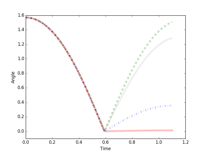
Figure 6 shows the result of this strategy applied to a pendulum system, now using a minimal coordinate (θ,θ˙)𝜃˙𝜃(\theta,\dot{\theta}) representation; assuming that the positive y𝑦y-axis points upward, θ=0𝜃0\theta=0 is defined such that the pendulum bob configuration is closest to y=𝑦y=-\infty. The pendulum is subject to a soft range of motion limit, imposing θ0𝜃0\theta\geq 0. This example system was simulated from the initial conditions {θ=π2,θ˙=0}formulae-sequence𝜃𝜋2˙𝜃0\{\theta=\frac{\pi}{2},\dot{\theta}=0\}.

Figure 6 shows that this system can be simulated stably with large step sizes; as expected, accuracy increases linearly as hh decreases.

Refer to caption
Figure 6: A plot of the pendulum with range of limit constraint at θ=0𝜃0\theta=0, with k=1012𝑘superscript1012k=10^{12} and b=0𝑏0b=0 simulated with h=105superscript105h=10^{-5} (red, solid), h=106superscript106h=10^{-6} (blue, dashed-dotted), h=107superscript107h=10^{-7} (grey, dotted) and h=108superscript108h=10^{-8} (green, dashed). While the system can be simulated stably for any value of hh, the true, elastic behavior is not evident until the step size becomes small; for values h105superscript105h\geq 10^{-5}, the impact against the range-of-motion limit appears to be “dead”.

5.5 Example: box on an elastic foundation

As a second example that will illustrate pathological worst-case performance for our method, consider a rigid cube (with side length s=1𝑠1s=1m and density 888kg//m3) resting on an elastic foundation (e.g., Winkler model) of depth 1m with a variable number of elements ({ 100, 900 }). Assume that the contact is frictionless. The system is simulated for one second of virtual time, starting from the box resting (zero velocity) on top of the elastic foundation at full extension (no deformation). I modeled the foundation as very stiff, using Young’s Modulus values of E=1011𝐸superscript1011E=10^{11} N/m2 (about that of steel) and E=107𝐸superscript107E=10^{7} N/m2 (about that of rubber) and a damping value of B=INsm𝐵𝐼NsmB=I\frac{\textrm{N}\cdot\textrm{s}}{\textrm{m}}. Note that increasing the number of elastic elements from 100 to 900 decreases the stiffness (K𝐾K) of each element in the foundation. K𝐾K is easily determined by multiplying the Young’s Modulus by the (uniform) element area and dividing by the depth of the foundation.

I additionally applied a force (of variable magnitude { 5N, 50N }) to the top of the cube at the point s/2[cos(10t)sin(10t)1]𝖳𝑠2superscriptmatrix10𝑡10𝑡1𝖳s/2{\begin{bmatrix}\cos{(10t)}&\sin{(10t)}&1\end{bmatrix}}^{\mathsf{T}} (in the cube frame). The force is directed downward (i.e., it is always in the direction of gravity). The constraint-based approach was tested against MATLAB’s ode15s implicit integrator, which I set to run in first-order for a equal comparison. I also validated the results using MATLAB’s ode45, which provides a high accuracy solution. I used a step size of 0.010.010.01s for both my constraint-based approach and MATLAB’s integrators.

Table 1 summarizes the timing results, which I will now discuss . First, the 555N force results in a steady-state solution, which ode15s is able to exploit. Indeed, the integrator requires essentially the same computational time to simulate to the designated end time (1s) or nearly any time beyond that. On the other hand, the 505050N force does not yield a steady state solution: the applied force causes a rocking behavior where the side of the cube opposite the point of application to separate slightly from the foundation. The result is that the ode15s runs much slower on this scenario.

Table 1 also highlights the disparity in running times when the number of elements is increased. The constraint-based approach scales cubically with the number of elements. The running time of ode15s is dominated by a O(m2)f(n)𝑂superscript𝑚2𝑓𝑛O(m^{2})f(n) factor to form the necessary Jacobian matrix, where m𝑚m is the number of velocity variables and f(n)𝑓𝑛f(n) is the running time of the collision detection algorithm. The collision detection algorithm for this particular example is relatively inexpensive and runs in linear time in the number of elements. The reason that implicit integrators like ode15s are fast at integrating steady state problems is because the Jacobian matrices can be reused. For the non-steady state problem, the Jacobians may require regular reconstruction (which requires significant computation), in which case the constraint-based method may be faster even when many elastic elements are used.

I note that the constraint-based method works reasonably well on all problems. It does not run for thousands of seconds on any of the examples. Its running time suffers from neither computational stiffness nor rapidly changing dynamics; it scales predictably as the number of constraints increase. Additionally, we can imagine re-using Jacobian matrices, applying warm starting, and employing other computational tricks that MATLAB’s mature ODE integrators exploit for solving initial value problems.

E=107𝐸superscript107E=10^{7} N/m2superscript𝑚2m^{2} E=1011𝐸superscript1011E=10^{11} N/m2superscript𝑚2m^{2}
elastic load constraint-based ode15s ode45 constraint-based ode15s ode45
elements approach approach
100 5N 0.331s 0.302s 28.0s 0.286s 0.189s 27.4s
100 50N 0.332s 9.55s 15.5s 0.396s 5550s 621s
900 5N 7.40s 4.75s 829s 8.23s 1.10s 17100s
900 50N 12.98s 27.3s 346s 26.00s 2.31s 17400s
Table 1: Timings (in seconds) to simulate the cube-on-elastic-foundation scenario with both the constraint-based approach and other integration techniques.

The error of the constraint-based approach with h=0.010.01h=0.01 on the elastic foundation problem is provided in Table 2. I compared final states against those obtained from ode45: it’s locally accurate to fourth-order and uses error control, and I have treated it as the ground truth. Absolute and relative errors are computed after one second of simulation time. These errors represent the Euclidean norm of the generalized coordinates (position and orientation) of the rigid body. The first four rows of the table show that absolute and relative error are quite good when the scenario is not particularly dynamic (follows from little loading). The last four rows of the table show significant error, though not instability.
Refer to caption
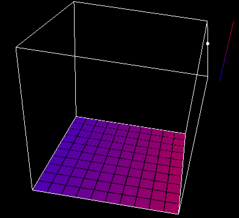
Figure 7: Depiction of forces on the cube/elastic-foundation example described in §5.5. The small white sphere on the upper right corner of the cube shows the point of application of the external, sinusoidal force. The magenta coloring of the elastic foundation elements indicate that pressure is greater on the right side of the box, as expected (pressure is not concentrated under the point of application since the box is modeled as rigid).

With respect to modeling breadth, Figure 7 shows that the constraint based approach is able to reasonably simulate compliant contact, including generating cogent pressure distributions. In the next section, we will see that the constraint-based approach can simulate Coulomb friction without increasing computational hardness and with minimal creep, which a purely ODE-based approach would struggle to effect efficiently.

Load Number of elements Elastic modulus (N/m2superscript𝑚2m^{2}) Absolute error Relative error
5 100 E=107𝐸superscript107E=10^{7} 2.96×1052.96superscript1052.96\times 10^{-5} 2.65×1052.65superscript1052.65\times 10^{-5}
5 100 E=1011𝐸superscript1011E=10^{11} 2.91×1072.91superscript1072.91\times 10^{-7} 2.60×1072.60superscript1072.60\times 10^{-7}
5 900 E=107𝐸superscript107E=10^{7} 1.98×1051.98superscript1051.98\times 10^{-5} 1.77×1051.77superscript1051.77\times 10^{-5}
5 900 E=1011𝐸superscript1011E=10^{11} 2.71×1092.71superscript1092.71\times 10^{-9} 2.42×1092.42superscript1092.42\times 10^{-9}
50 100 E=107𝐸superscript107E=10^{7} 0.8130.8130.813 0.7240.7240.724
50 100 E=1011𝐸superscript1011E=10^{11} 0.8140.8140.814 0.7280.7280.728
50 900 E=107𝐸superscript107E=10^{7} 1.0×1021.0superscript1021.0\times 10^{-2} 8.87×1038.87superscript1038.87\times 10^{-3}
50 900 E=1011𝐸superscript1011E=10^{11} 1.0×1021.0superscript1021.0\times 10^{-2} 8.95×1038.95superscript1038.95\times 10^{-3}
Table 2: Accuracy for the constraint-based approach at h=102superscript102h=10^{-2}. Error compared against ode45. Error improves significantly for h=103superscript103h=10^{-3} (not listed above); the absolute errors for 100 elements with E=107𝐸superscript107E=10^{7} N/m2superscript𝑚2m^{2} (fifth row) and E=1011𝐸superscript1011E=10^{1}1 N/m2superscript𝑚2m^{2} (sixth row) drop to 3.14×1033.14superscript1033.14\times 10^{-3} and 9.22×1059.22superscript1059.22\times 10^{-5}, respectively.

6 Modeling Contact with Coulomb friction

The path to modeling contact and friction extends the concept described in the previous section. Assume that the unilateral constraint from that section now models two bodies contacting over a surface, and that ϕnsubscriptitalic-ϕ𝑛\phi_{n}\to\mathbb{R} corresponds to the signed depth of indentation; for sake of ready interpretability and without lack of generality, consider one of the bodies to be rigid and the other to be compliant. The unilateral constraint,

M^nϕ¨n+Bϕ˙n+Kϕn=f^n,subscript^𝑀𝑛subscript¨italic-ϕ𝑛𝐵subscript˙italic-ϕ𝑛𝐾subscriptitalic-ϕ𝑛subscript^𝑓𝑛\displaystyle\hat{M}_{n}\ddot{\phi}_{n}+B\dot{\phi}_{n}+K\phi_{n}=\hat{f}_{n}, (86)

introduces “n” subscripts for the variables above to help us distinguish them from other variables later on this section. This constraint prescribes the stiffness and damping in the direction of the surface normal, which results in the integral of the pressure over the surface, and this integral will be denoted λnsubscript𝜆𝑛\lambda_{n}. The pressure at any point on that surface would then be given by λnasubscript𝜆𝑛𝑎\frac{\lambda_{n}}{a}, where a𝑎a is the area of the contact surface. Like the elastic foundation example in the previous section, the contact surface can be divided into numbers of discrete elements in order to approximate the pressure distribution with greater accuracy.

But let us return to considering a single spring element representing the surface deformation. Assuming that the contact exists in the context of a 2D system, a second spring—acting orthogonally to the first spring—can model Coulomb friction (see Figure 8); I will denote this constraint ϕrsubscriptitalic-ϕ𝑟\phi_{r} (and its corresponding force λrsubscript𝜆𝑟\lambda_{r}). If the contact exists in the context of a 3D system, two such orthogonal springs would be necessary: one for each of two basis directions orthogonal to the first spring. The two (or three) spring-dampers corresponding to each spring-damper element can be imagined as connected in series (also shown in Figure 8).
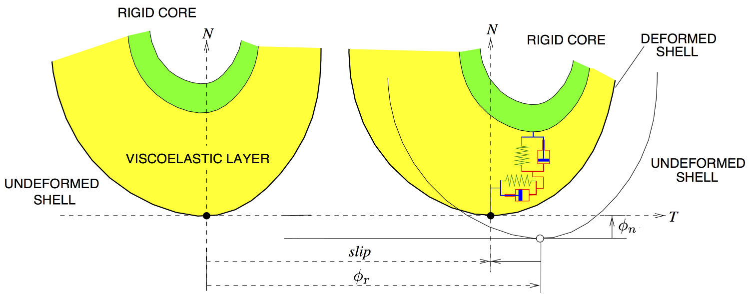
Refer to caption
Figure 8: A depiction of the model in [20] (illustration adapted from there as well), with the normal and tangential deformations to the surface normal at a presumed point of contact (the case of the deformation, i.e., a contact with another body, is not shown). Note that the virtual springs lie in series.

Song et al. [20] was the first to propose this particular model of compliant contact, to my knowledge. To concretize the meaning of the constraints:

  • ϕn0subscriptitalic-ϕ𝑛0\phi_{n}\leq 0 represents the negated amount of deformation along the contact normal between two bodies at a point of contact. Disjoint (i.e., not touching) bodies do not deform, in which case ϕ=0italic-ϕ0\phi=0. Lacoursiere noted that ϕnsubscriptitalic-ϕ𝑛\phi_{n} can also represent a negated potential energy function [17].

  • ϕn˙˙subscriptitalic-ϕ𝑛\dot{\phi_{n}} represents the rate of deformation along the contact normal between two bodies at a point of contact. ϕ˙>0˙italic-ϕ0\dot{\phi}>0 indicates that deformation is decreasing. For two rigid bodies (i.e., k=𝑘k=\infty), ϕn˙˙subscriptitalic-ϕ𝑛\dot{\phi_{n}} represents the relative velocity at the point of contact projected along the contact normal, where positive ϕ˙˙italic-ϕ\dot{\phi} indicates that two bodies are moving apart at the point of contact.

  • ϕrsubscriptitalic-ϕ𝑟\phi_{r} represents the amount of signed deformation orthogonal to the contact normal between two bodies at a point of contact.

  • ϕr˙˙subscriptitalic-ϕ𝑟\dot{\phi_{r}} represents the rate of deformation orthogonal to the contact normal between two bodies at a point of contact. For two rigid bodies, ϕr˙˙subscriptitalic-ϕ𝑟\dot{\phi_{r}} represents the relative velocity at the point of contact projected orthogonal to the contact normal. ϕ˙r=0subscript˙italic-ϕ𝑟0\dot{\phi}_{r}=0 and ϕ˙r0subscript˙italic-ϕ𝑟0\dot{\phi}_{r}\neq 0 correspond to bodies sticking/rolling and sliding, respectively, at the point of contact.

As was the case in the previous section, we will typically not track (integrate) ϕnsubscriptitalic-ϕ𝑛\phi_{n}, ϕ˙nsubscript˙italic-ϕ𝑛\dot{\phi}_{n}, ϕrsubscriptitalic-ϕ𝑟\phi_{r}, and ϕ˙rsubscript˙italic-ϕ𝑟\dot{\phi}_{r} directly. ϕnsubscriptitalic-ϕ𝑛\phi_{n}, ϕ˙nsubscript˙italic-ϕ𝑛\dot{\phi}_{n}, and ϕ˙rsubscript˙italic-ϕ𝑟\dot{\phi}_{r} are often computed using the state (q,v)𝑞𝑣(q,v) of the multibody system: for q𝑞q corresponding to overlapping undeformed geometries, a mapping to a kissing, deformed configuration will be computed from which ϕnsubscriptitalic-ϕ𝑛\phi_{n}, ϕ˙nsubscript˙italic-ϕ𝑛\dot{\phi}_{n}, and ϕ˙rsubscript˙italic-ϕ𝑟\dot{\phi}_{r} can be computed. ϕrsubscriptitalic-ϕ𝑟\phi_{r} could be tracked by augmenting the system’s state variables, but this can be avoided by making the friction model memoryless (discussed immediately below).

6.1 DPP formulation of a contact constrained system with Coulomb friction, (applicable for ϕn0subscriptitalic-ϕ𝑛0\phi_{n}\leq 0)

I focus on Coulomb friction rather than another friction model because the former is simple and captures important stick-slip transitions. It also does not incorporate tangential deformation “memory”, which simplifies the model and its implementation significantly. In keeping with this simple model of friction, I avoid discriminating between sticking and sliding friction states, which simplifies both the contact model and its implementation. That lack of discrimination causes the differential equations for the constraint dynamics (the ϕitalic-ϕ\phi variables) to become numerically stiff (see [21]), which does not hamper the efficiency of my implicit approach. The DPP model of a contact constrained with Coulomb friction using my scheme follows:

minλn,λr,ϕn,ϕ˙n,ϕr,ϕ˙r,βrsubscriptminsubscript𝜆𝑛subscript𝜆𝑟subscriptitalic-ϕ𝑛subscript˙italic-ϕ𝑛subscriptitalic-ϕ𝑟subscript˙italic-ϕ𝑟subscript𝛽𝑟\displaystyle\operatorname*{min}_{\lambda_{n},\lambda_{r},\phi_{n},\dot{\phi}_{n},\phi_{r},\dot{\phi}_{r},\beta_{r}}\ 12λn𝖳λn+12λr𝖳λr+12βr𝖳βr12superscriptsubscript𝜆𝑛𝖳subscript𝜆𝑛12superscriptsubscript𝜆𝑟𝖳subscript𝜆𝑟12superscriptsubscript𝛽𝑟𝖳subscript𝛽𝑟\displaystyle\frac{1}{2}{\lambda_{n}}^{\mathsf{T}}\lambda_{n}+\frac{1}{2}{\lambda_{r}}^{\mathsf{T}}\lambda_{r}+\frac{1}{2}{\beta_{r}}^{\mathsf{T}}{\beta_{r}} (87)
q˙=˙𝑞absent\displaystyle\dot{q}= Nv𝑁𝑣\displaystyle\ Nv (88)
Mv˙=𝑀˙𝑣absent\displaystyle M\dot{v}= Gn𝖳λn+Gr𝖳λr+fsuperscriptsubscript𝐺𝑛𝖳subscript𝜆𝑛superscriptsubscript𝐺𝑟𝖳subscript𝜆𝑟𝑓\displaystyle\ {G_{n}}^{\mathsf{T}}\lambda_{n}+{G_{r}}^{\mathsf{T}}\lambda_{r}+f (89)
f^n=subscript^𝑓𝑛absent\displaystyle\hat{f}_{n}= M^nϕ¨n+Bϕ˙n+Kϕnsubscript^𝑀𝑛subscript¨italic-ϕ𝑛𝐵subscript˙italic-ϕ𝑛𝐾subscriptitalic-ϕ𝑛\displaystyle\ \hat{M}_{n}\ddot{\phi}_{n}+B\dot{\phi}_{n}+K\phi_{n} (90)
f^r=subscript^𝑓𝑟absent\displaystyle\hat{f}_{r}= M^rϕ¨r+Bϕ˙r+Kϕrsubscript^𝑀𝑟subscript¨italic-ϕ𝑟𝐵subscript˙italic-ϕ𝑟𝐾subscriptitalic-ϕ𝑟\displaystyle\ \hat{M}_{r}\ddot{\phi}_{r}+B\dot{\phi}_{r}+K\phi_{r} (91)
λnsubscript𝜆𝑛absent\displaystyle\lambda_{n}\geq KnϕnBnϕ˙nM^nG˙nvsubscript𝐾𝑛subscriptitalic-ϕ𝑛subscript𝐵𝑛subscript˙italic-ϕ𝑛subscript^𝑀𝑛subscript˙𝐺𝑛𝑣\displaystyle-K_{n}\phi_{n}-B_{n}\dot{\phi}_{n}-\hat{M}_{n}\dot{G}_{n}v (92)
λnsubscript𝜆𝑛absent\displaystyle\lambda_{n}\geq 00\displaystyle\ 0 (93)
λr=subscript𝜆𝑟absent\displaystyle\lambda_{r}= KrϕrBrϕ˙rM^rG˙rv+βrsubscript𝐾𝑟subscriptitalic-ϕ𝑟subscript𝐵𝑟subscript˙italic-ϕ𝑟subscript^𝑀𝑟subscript˙𝐺𝑟𝑣subscript𝛽𝑟\displaystyle-K_{r}\phi_{r}-B_{r}\dot{\phi}_{r}-\hat{M}_{r}\dot{G}_{r}v+\beta_{r} (94)
λrsubscript𝜆𝑟absent\displaystyle\lambda_{r}\leq μλn𝜇subscript𝜆𝑛\displaystyle\ \mu\lambda_{n} (95)
λrsubscript𝜆𝑟absent\displaystyle-\lambda_{r}\leq μλn.𝜇subscript𝜆𝑛\displaystyle\ \mu\lambda_{n}. (96)

Similarities between the last QP and (88)–(90) and (92)–(93) in this QP should be evident. The novel equations are (91) which describes the tangential spring dynamics, (95) and (96) which limit the amount of frictional force according to the Coulomb friction model, and (94); the latter will be discussed in detail below. Another difference from the last QP includes separate stiffness/damping terms for normal and tangential directions (Kn/Bnsubscript𝐾𝑛subscript𝐵𝑛K_{n}/B_{n} and Kr/Brsubscript𝐾𝑟subscript𝐵𝑟K_{r}/B_{r}, respectively).

Neither problem feasibility nor convexity of the above QP will be analyzed here. A time-discretized, more general version (extended with 3D friction constraints, bilateral constraints, and generic unilateral constraints) of the QP-based method introduced immediately below will be analyzed in Appendix 0.A and found to be feasible and strictly convex. But for now, we examine the presence of the βrsubscript𝛽𝑟\beta_{r} term in  (94) by first noting that the nominal constraints for λrsubscript𝜆𝑟\lambda_{r}, i.e.,

λr=KrϕrBrϕ˙rM^rG˙rvsubscript𝜆𝑟subscript𝐾𝑟subscriptitalic-ϕ𝑟subscript𝐵𝑟subscript˙italic-ϕ𝑟subscript^𝑀𝑟subscript˙𝐺𝑟𝑣\displaystyle\lambda_{r}=-K_{r}\phi_{r}-B_{r}\dot{\phi}_{r}-\hat{M}_{r}\dot{G}_{r}v\qquad (spring/damper behavior) (97)
|λr|μλnsubscript𝜆𝑟𝜇subscript𝜆𝑛\displaystyle|\lambda_{r}|\leq\mu\lambda_{n}\qquad (Coulomb friction), (98)

generally conflict. In response, we enforce one “hard” constraint (Coulomb friction) and one “soft” one (the spring-damper like behavior) along the contact tangent; the QP finds the frictional forces that respect Coulomb friction yet come as close to the desired damped, oscillatory behavior by introducing the βrsubscript𝛽𝑟\beta_{r} term into (97), yielding  (94). This desired behavior is encouraged by the objective function (Equation 87), which quadratically penalizes the βrsubscript𝛽𝑟\beta_{r} term.

Examining the objective function in detail, notice that each dimension of λnsubscript𝜆𝑛\lambda_{n}, λrsubscript𝜆𝑟\lambda_{r}, and βrsubscript𝛽𝑟\beta_{r} corresponds to consistent units (e.g., Newtons). Although the units are consistent, it might be conceivable that the solution to the QP increases λnsubscript𝜆𝑛\lambda_{n} in order to decrease βrsubscript𝛽𝑟\beta_{r}. However, the criteria λn𝖳λnsuperscriptsubscript𝜆𝑛𝖳subscript𝜆𝑛{\lambda_{n}}^{\mathsf{T}}\lambda_{n} and βr𝖳βrsuperscriptsubscript𝛽𝑟𝖳subscript𝛽𝑟{\beta_{r}}^{\mathsf{T}}\beta_{r} should not be equally valued in the optimization: the former term penalizes deviation from the nonlinear equality constraint λn=max(0,KnϕnBnϕ˙nM^nG˙nv)subscript𝜆𝑛0subscript𝐾𝑛subscriptitalic-ϕ𝑛subscript𝐵𝑛subscript˙italic-ϕ𝑛subscript^𝑀𝑛subscript˙𝐺𝑛𝑣\lambda_{n}=\max{(0,-K_{n}\phi_{n}-B_{n}\dot{\phi}_{n}-\hat{M}_{n}\dot{G}_{n}v}), so a significant weight (penalty) should be assigned to the term λn𝖳λnsuperscriptsubscript𝜆𝑛𝖳subscript𝜆𝑛{\lambda_{n}}^{\mathsf{T}}\lambda_{n} (I used 1/h11/h in my implementation so as to obtain greater accuracy as hh is decreased), while keeping the weights of all other terms to unity. This weighting factor will be introduced using the term ζ𝜁\zeta.

6.2 The time-discretized DPP (for contact problems in 2D)

After we discretize in time, we can introduce specific discrete time variables to be determined via optimization. This quadratic program serves as the implicit integration scheme for ϕn,ϕ˙n,ϕrsubscriptitalic-ϕ𝑛subscript˙italic-ϕ𝑛subscriptitalic-ϕ𝑟\phi_{n},\dot{\phi}_{n},\phi_{r}, and ϕ˙rsubscript˙italic-ϕ𝑟\dot{\phi}_{r}. As in Section 5.3, the constraint dynamics described in (90) and (91) are redundant and need not be considered further. Also as in Section 5.3: once λn1subscript𝜆subscript𝑛1\lambda_{n_{1}} and λr1subscript𝜆subscript𝑟1\lambda_{r_{1}} have been computed, then v1subscript𝑣1v_{1} and q1subscript𝑞1q_{1} are found by evaluating v1=v0+hM𝟣(Gn𝖳λn1+Gr𝖳λr1+f)subscript𝑣1subscript𝑣0superscript𝑀1superscriptsubscript𝐺𝑛𝖳subscript𝜆subscript𝑛1superscriptsubscript𝐺𝑟𝖳subscript𝜆subscript𝑟1𝑓v_{1}=v_{0}+h{M}^{\mathsf{-1}}({G_{n}}^{\mathsf{T}}\lambda_{n_{1}}+{G_{r}}^{\mathsf{T}}\lambda_{r_{1}}+f) and q1=q0+hNv1subscript𝑞1subscript𝑞0𝑁subscript𝑣1q_{1}=q_{0}+hNv_{1}.

minλn1,λr1,ϕn1,ϕ˙n1,ϕr1,ϕ˙r1,βrsubscriptminsubscript𝜆subscript𝑛1subscript𝜆subscript𝑟1subscriptitalic-ϕsubscript𝑛1subscript˙italic-ϕsubscript𝑛1subscriptitalic-ϕsubscript𝑟1subscript˙italic-ϕsubscript𝑟1subscript𝛽𝑟\displaystyle\operatorname*{min}_{\lambda_{n_{1}},\lambda_{r_{1}},\phi_{n_{1}},\dot{\phi}_{n_{1}},\phi_{r_{1}},\dot{\phi}_{r_{1}},\beta_{r}}\ ζ2λn1𝖳λn1+12λr1𝖳λr1+12βr𝖳βr𝜁2superscriptsubscript𝜆subscript𝑛1𝖳subscript𝜆subscript𝑛112superscriptsubscript𝜆subscript𝑟1𝖳subscript𝜆subscript𝑟112superscriptsubscript𝛽𝑟𝖳subscript𝛽𝑟\displaystyle\frac{\zeta}{2}{\lambda_{n_{1}}}^{\mathsf{T}}\lambda_{n_{1}}+\frac{1}{2}{\lambda_{r_{1}}}^{\mathsf{T}}\lambda_{r_{1}}+\frac{1}{2}{\beta_{r}}^{\mathsf{T}}{\beta_{r}} (99)
ϕn1=subscriptitalic-ϕsubscript𝑛1absent\displaystyle\phi_{n_{1}}= ϕn0+hϕ˙n1+O(h2)subscriptitalic-ϕsubscript𝑛0subscript˙italic-ϕsubscript𝑛1𝑂superscript2\displaystyle\ \phi_{n_{0}}+h\dot{\phi}_{n_{1}}+O(h^{2}) (100)
ϕ˙n1=subscript˙italic-ϕsubscript𝑛1absent\displaystyle\dot{\phi}_{n_{1}}= ϕ˙n0+hϕ¨n0+O(h2)subscript˙italic-ϕsubscript𝑛0subscript¨italic-ϕsubscript𝑛0𝑂superscript2\displaystyle\ \dot{\phi}_{n_{0}}+h\ddot{\phi}_{n_{0}}+O(h^{2}) (101)
ϕr1=subscriptitalic-ϕsubscript𝑟1absent\displaystyle\phi_{r_{1}}= ϕr0+hϕ˙r1+O(h2)subscriptitalic-ϕsubscript𝑟0subscript˙italic-ϕsubscript𝑟1𝑂superscript2\displaystyle\ \phi_{r_{0}}+h\dot{\phi}_{r_{1}}+O(h^{2}) (102)
ϕ˙r1=subscript˙italic-ϕsubscript𝑟1absent\displaystyle\dot{\phi}_{r_{1}}= ϕ˙r0+hϕ¨r0+O(h2)subscript˙italic-ϕsubscript𝑟0subscript¨italic-ϕsubscript𝑟0𝑂superscript2\displaystyle\ \dot{\phi}_{r_{0}}+h\ddot{\phi}_{r_{0}}+O(h^{2}) (103)
λn1subscript𝜆subscript𝑛1absent\displaystyle\lambda_{n_{1}}\geq Knϕn1Bnϕ˙n1M^nG˙nv0+O(h)subscript𝐾𝑛subscriptitalic-ϕsubscript𝑛1subscript𝐵𝑛subscript˙italic-ϕsubscript𝑛1subscript^𝑀𝑛subscript˙𝐺𝑛subscript𝑣0𝑂\displaystyle-K_{n}\phi_{n_{1}}-B_{n}\dot{\phi}_{n_{1}}-\hat{M}_{n}\dot{G}_{n}v_{0}+O(h) (104)
λn1subscript𝜆subscript𝑛1absent\displaystyle\lambda_{n_{1}}\geq 00\displaystyle\ 0 (105)
λr1=subscript𝜆subscript𝑟1absent\displaystyle\lambda_{r_{1}}= Krϕr1Brϕ˙r1M^rG˙rv0+βr+O(h)subscript𝐾𝑟subscriptitalic-ϕsubscript𝑟1subscript𝐵𝑟subscript˙italic-ϕsubscript𝑟1subscript^𝑀𝑟subscript˙𝐺𝑟subscript𝑣0subscript𝛽𝑟𝑂\displaystyle-K_{r}\phi_{r_{1}}-B_{r}\dot{\phi}_{r_{1}}-\hat{M}_{r}\dot{G}_{r}v_{0}+\beta_{r}+O(h) (106)
λr1subscript𝜆subscript𝑟1absent\displaystyle\lambda_{r_{1}}\leq μλn1𝜇subscript𝜆subscript𝑛1\displaystyle\ \mu\lambda_{n_{1}} (107)
λr1subscript𝜆subscript𝑟1absent\displaystyle-\lambda_{r_{1}}\leq μλn1.𝜇subscript𝜆subscript𝑛1\displaystyle\ \mu\lambda_{n_{1}}. (108)

I will show in Appendix 0.A that the “free” problem variables (ϕn1,ϕ˙n1,ϕr1,ϕ˙r1subscriptitalic-ϕsubscript𝑛1subscript˙italic-ϕsubscript𝑛1subscriptitalic-ϕsubscript𝑟1subscript˙italic-ϕsubscript𝑟1\phi_{n_{1}},\dot{\phi}_{n_{1}},\phi_{r_{1}},\dot{\phi}_{r_{1}}, and βrsubscript𝛽𝑟\beta_{r}) can be eliminated, reducing the problem to a purely inequality constrained QP in many fewer variables (two in this case: λn1subscript𝜆subscript𝑛1\lambda_{n_{1}} and λr1subscript𝜆subscript𝑟1\lambda_{r_{1}}). Appendix 0.A also shows that the QP is both feasible and strictly convex.

We will next discuss contact problems in 3D. Before we do, note that the Coulomb friction constraints (e.g., Equations 95 and 96) do not specify which direction the force should be applied. If the friction model is truly Coulomb, however, it will be memory-less (implying Kr=0subscript𝐾𝑟0K_{r}=0); in that case, λr1subscript𝜆subscript𝑟1\lambda_{r_{1}} will oppose ϕ˙r1subscript˙italic-ϕsubscript𝑟1\dot{\phi}_{r_{1}}, as consistent with the principle of maximum power [9] from the Coulomb friction model. In other words, setting Kr=0subscript𝐾𝑟0K_{r}=0 allows the model to faithfully emulate the Coulomb friction model.

6.3 Three-dimensional contact

In the three dimensional contact version, we add three more variables per point contact between two bodies—ϕs1subscriptitalic-ϕsubscript𝑠1\phi_{s_{1}}, ϕ˙s1subscript˙italic-ϕsubscript𝑠1\dot{\phi}_{s_{1}}, and λs1subscript𝜆subscript𝑠1\lambda_{s_{1}}— which correspond to deformation, deformation time derivative, and applied force for the spring-damper in a second basis direction orthogonal to the contact normal (the spring-damper corresponding to the r𝑟r index is in another such basis direction). We also need to account for a proper friction “cone”, as was done using two inequality constraints in (95) and (96); this will be effected using a quadratic constraint for each of the m𝑚m points of contact. Other than this constraint, the now quadratically constrained quadratic program (QCQP) will appear much like the quadratic program used in the DPP from the last section:

minλ1,ϕ1,ϕ˙1,βr,βssubscriptminsubscript𝜆subscript1subscriptitalic-ϕsubscript1subscript˙italic-ϕsubscript1subscript𝛽𝑟subscript𝛽𝑠\displaystyle\operatorname*{min}_{\lambda_{*_{1}},\phi_{*_{1}},\dot{\phi}_{*_{1}},\beta_{r},\beta_{s}} ζ2λn1𝖳λn1+12λr1𝖳λr1+12λs1𝖳λs1+𝜁2superscriptsubscript𝜆subscript𝑛1𝖳subscript𝜆subscript𝑛112superscriptsubscript𝜆subscript𝑟1𝖳subscript𝜆subscript𝑟112superscriptsubscript𝜆subscript𝑠1𝖳subscript𝜆subscript𝑠1\displaystyle\frac{\zeta}{2}{\lambda_{n_{1}}}^{\mathsf{T}}\lambda_{n_{1}}+\frac{1}{2}{\lambda_{r_{1}}}^{\mathsf{T}}\lambda_{r_{1}}+\frac{1}{2}{\lambda_{s_{1}}}^{\mathsf{T}}\lambda_{s_{1}}+\ldots
12βr𝖳βr+12βs𝖳βs12superscriptsubscript𝛽𝑟𝖳subscript𝛽𝑟12superscriptsubscript𝛽𝑠𝖳subscript𝛽𝑠\displaystyle\frac{1}{2}{\beta_{r}}^{\mathsf{T}}{\beta_{r}}+\frac{1}{2}{\beta_{s}}^{\mathsf{T}}{\beta_{s}} (109)
q˙1=subscript˙𝑞1absent\displaystyle\dot{q}_{1}= Nv1+O(h2)𝑁subscript𝑣1𝑂superscript2\displaystyle\ Nv_{1}+O(h^{2})
Mv˙0=𝑀subscript˙𝑣0absent\displaystyle M\dot{v}_{0}= Gn𝖳λn1+Gr𝖳λr1+Gs𝖳λs1+f+O(h)superscriptsubscript𝐺𝑛𝖳subscript𝜆subscript𝑛1superscriptsubscript𝐺𝑟𝖳subscript𝜆subscript𝑟1subscriptsuperscript𝐺𝖳𝑠subscript𝜆subscript𝑠1𝑓𝑂\displaystyle\ {G_{n}}^{\mathsf{T}}\lambda_{n_{1}}+{G_{r}}^{\mathsf{T}}\lambda_{r_{1}}+{G}^{\mathsf{T}}_{s}\lambda_{s_{1}}+f+O(h)
ϕn1=subscriptitalic-ϕsubscript𝑛1absent\displaystyle\phi_{n_{1}}= ϕn0+hϕ˙n1+O(h2)subscriptitalic-ϕsubscript𝑛0subscript˙italic-ϕsubscript𝑛1𝑂superscript2\displaystyle\phi_{n_{0}}+h\dot{\phi}_{n_{1}}+O(h^{2}) (110)
ϕ˙n1=subscript˙italic-ϕsubscript𝑛1absent\displaystyle\dot{\phi}_{n_{1}}= ϕ˙n0+hϕ¨n0+O(h2)subscript˙italic-ϕsubscript𝑛0subscript¨italic-ϕsubscript𝑛0𝑂superscript2\displaystyle\dot{\phi}_{n_{0}}+h\ddot{\phi}_{n_{0}}+O(h^{2}) (111)
ϕr1=subscriptitalic-ϕsubscript𝑟1absent\displaystyle\phi_{r_{1}}= ϕr0+hϕ˙r1+O(h2)subscriptitalic-ϕsubscript𝑟0subscript˙italic-ϕsubscript𝑟1𝑂superscript2\displaystyle\phi_{r_{0}}+h\dot{\phi}_{r_{1}}+O(h^{2}) (112)
ϕ˙r1=subscript˙italic-ϕsubscript𝑟1absent\displaystyle\dot{\phi}_{r_{1}}= ϕ˙r0+hϕ¨r0+O(h2)subscript˙italic-ϕsubscript𝑟0subscript¨italic-ϕsubscript𝑟0𝑂superscript2\displaystyle\dot{\phi}_{r_{0}}+h\ddot{\phi}_{r_{0}}+O(h^{2}) (113)
ϕs1=subscriptitalic-ϕsubscript𝑠1absent\displaystyle\phi_{s_{1}}= ϕs0+hϕ˙s1+O(h2)subscriptitalic-ϕsubscript𝑠0subscript˙italic-ϕsubscript𝑠1𝑂superscript2\displaystyle\phi_{s_{0}}+h\dot{\phi}_{s_{1}}+O(h^{2}) (114)
ϕ˙s1=subscript˙italic-ϕsubscript𝑠1absent\displaystyle\dot{\phi}_{s_{1}}= ϕ˙s0+hϕ¨s0+O(h2)subscript˙italic-ϕsubscript𝑠0subscript¨italic-ϕsubscript𝑠0𝑂superscript2\displaystyle\dot{\phi}_{s_{0}}+h\ddot{\phi}_{s_{0}}+O(h^{2}) (115)
λn1subscript𝜆subscript𝑛1absent\displaystyle\lambda_{n_{1}}\geq Knϕn1Bnϕ˙n1M^nG˙nv0+O(h)subscript𝐾𝑛subscriptitalic-ϕsubscript𝑛1subscript𝐵𝑛subscript˙italic-ϕsubscript𝑛1subscript^𝑀𝑛subscript˙𝐺𝑛subscript𝑣0𝑂\displaystyle-K_{n}\phi_{n_{1}}-B_{n}\dot{\phi}_{n_{1}}-\hat{M}_{n}\dot{G}_{n}v_{0}+O(h) (116)
λn1subscript𝜆subscript𝑛1absent\displaystyle\lambda_{n_{1}}\geq 00\displaystyle\ 0 (117)
λr1=subscript𝜆subscript𝑟1absent\displaystyle\lambda_{r_{1}}= Krϕr1Brϕ˙r1M^rG˙rv0+βr+O(h)subscript𝐾𝑟subscriptitalic-ϕsubscript𝑟1subscript𝐵𝑟subscript˙italic-ϕsubscript𝑟1subscript^𝑀𝑟subscript˙𝐺𝑟subscript𝑣0subscript𝛽𝑟𝑂\displaystyle-K_{r}\phi_{r_{1}}-B_{r}\dot{\phi}_{r_{1}}-\hat{M}_{r}\dot{G}_{r}v_{0}+\beta_{r}+O(h) (118)
λs1=subscript𝜆subscript𝑠1absent\displaystyle\lambda_{s_{1}}= Ksϕs1Bsϕ˙s1M^sG˙sv0+βs+O(h)subscript𝐾𝑠subscriptitalic-ϕsubscript𝑠1subscript𝐵𝑠subscript˙italic-ϕsubscript𝑠1subscript^𝑀𝑠subscript˙𝐺𝑠subscript𝑣0subscript𝛽𝑠𝑂\displaystyle-K_{s}\phi_{s_{1}}-B_{s}\dot{\phi}_{s_{1}}-\hat{M}_{s}\dot{G}_{s}v_{0}+\beta_{s}+O(h) (119)
μi2λni2superscriptsubscript𝜇𝑖2superscriptsubscript𝜆subscript𝑛𝑖2\displaystyle\mu_{i}^{2}\lambda_{n_{i}}^{2} λri2+λsi2 for i=1,,m.formulae-sequenceabsentsuperscriptsubscript𝜆subscript𝑟𝑖2superscriptsubscript𝜆subscript𝑠𝑖2 for 𝑖1𝑚\displaystyle\geq\lambda_{r_{i}}^{2}+\lambda_{s_{i}}^{2}\textrm{ for }i=1,\ldots,m. (120)

where λ1subscript𝜆subscript1\lambda_{*_{1}} represents the variables λn1subscript𝜆subscript𝑛1\lambda_{n_{1}}, λr1subscript𝜆subscript𝑟1\lambda_{r_{1}} and λs1subscript𝜆subscript𝑠1\lambda_{s_{1}}; ϕ1subscriptitalic-ϕsubscript1\phi_{*_{1}} represents the variables ϕn1subscriptitalic-ϕsubscript𝑛1\phi_{n_{1}}, ϕr1subscriptitalic-ϕsubscript𝑟1\phi_{r_{1}}, and ϕs1subscriptitalic-ϕsubscript𝑠1\phi_{s_{1}}; and ϕ˙1subscript˙italic-ϕsubscript1\dot{\phi}_{*_{1}} represents the variables ϕ˙n1subscript˙italic-ϕsubscript𝑛1\dot{\phi}_{n_{1}}, ϕ˙r1subscript˙italic-ϕsubscript𝑟1\dot{\phi}_{r_{1}}, and ϕ˙s1subscript˙italic-ϕsubscript𝑠1\dot{\phi}_{s_{1}}.

6.4 Example: box on an inclined plane

Examples with contact and friction require greater sophistication than the very simple examples I have used prior to now. A good example with contact and friction should demonstrate multiple phenomena: (1) ​ no frictional forces are applied when μ=0𝜇0\mu=0; (2) ​ bodies remain in stiction given sufficiently large μ𝜇\mu; (3) ​ all other variables held constant, contacting bodies slide against each other farther with lower μ𝜇\mu; and (4) ​ frictional forces should oppose the direction of motion.

To demonstrate these phenomena, I implemented the equations above as a plugin for RPI-MATLAB-Simulator (using MATLAB R2015b) and tested their “sliding block” example, which consists of a box of unit mass, width 0.1m, length 0.2m, and height 0.05m that is initially motionless on a ramp inclined 15superscript1515^{\circ}. RPI-MATLAB-Simulator models the contact between the block and the ramp using point contacts, which means that the box should be conceived as having four spherical “feet” attached to its bottom. To simplify this example, we will model these feet as perfectly rigid and the ramp as an elastic halfspace, which will allow us to use Hertzian contact theory to determine the stiffness (Knsubscript𝐾𝑛K_{n}) for a given deformation, d𝑑d. Hertzian contact predicts the magnitude of the force from deformation as

f𝑓\displaystyle f =Erd3,absentsuperscript𝐸𝑟superscript𝑑3\displaystyle=E^{*}\sqrt{rd^{3}}, (121)

where Esuperscript𝐸E^{*} comprises relative moduli (Young’s Modulus and Poisson’s Ratio) and r𝑟r is the radius of the spherical feet. For this example problem, let us assume a radius of 0.01m. We now have the information with which to determine ϕnsubscriptitalic-ϕ𝑛\phi_{n} and Knsubscript𝐾𝑛K_{n}. Specifically, we will define the diagonal entries of Knsubscript𝐾𝑛K_{n} as

Kniisubscript𝐾subscript𝑛𝑖𝑖\displaystyle K_{n_{ii}} =Er,absentsuperscript𝐸𝑟\displaystyle=E^{*}\sqrt{r}, (122)

where we will assume that the elastic halfspace is comprised of a material with the rigidity of steel (recall that the feet are rigid), so Esuperscript𝐸E^{*} will be 100100100 GPa = 1011superscript101110^{11} N/m2superscriptN/m2\textrm{N/m}^{2}. r𝑟\sqrt{r} will be 110110\frac{1}{10} m1/2superscriptm12\textrm{m}^{1/2}, yielding a pseudo-stiffness of 1010superscript101010^{10} N/m1/2superscriptN/m12\textrm{N/m}^{1/2} (it is only a pseudo-stiffness because it is not quite in units of N/m). That is okay because we will define ϕnisubscriptitalic-ϕsubscript𝑛𝑖\phi_{n_{i}} (i𝑖i refers to the index of one of the spherical feet) to return units of m3/2superscriptm32\textrm{m}^{3/2} rather than m:

ϕnisubscriptitalic-ϕsubscript𝑛𝑖\displaystyle\phi_{n_{i}} =di3/2.absentsuperscriptsubscript𝑑𝑖32\displaystyle=d_{i}^{3/2}. (123)

RPI-MATLAB-Simulator provides the deformation depth, disubscript𝑑𝑖d_{i} for each contacting sphere/halfspace combination (it does not compute deformation for the block feet that are not in contact). Selecting damping parameters is never so straightforward; even for highly accurate models, damping must usually be set subjectively to realize qualitatively desired behavior. I set the diagonal entries of Bnsubscript𝐵𝑛B_{n} to unity as a guess to effect “a little damping”. I set the diagonal entries of Krsubscript𝐾𝑟K_{r} and Kssubscript𝐾𝑠K_{s} to zero to emulate the Coulomb friction model, which is memoryless as I noted earlier.

It should be clear that Brsubscript𝐵𝑟B_{r} and Bssubscript𝐵𝑠B_{s} (called B𝐵B in the remainder of this paragraph) should be set as large as possible. We want the friction coefficient to limit the force applied, not the dynamics of the virtual damper. Unfortunately, the numerical range of the optimization problem increases with B𝐵B: the number of digits of precision required is O(hB)𝑂𝐵O(hB), which can challenge the default tolerances used by some numerical libraries. I found that setting B=106h𝐵superscript106B=\frac{10^{6}}{h} meters results in no creep and no failed solves.

In the context of this example, I varied friction using μ={0,0.125,0.25,0.375}𝜇00.1250.250.375\mu=\{0,0.125,0.25,0.375\}. I guaranteed that there were no frictional forces applied when μ=0𝜇0\mu=0, and we observed the box remain in stiction at μ=0.375𝜇0.375\mu=0.375. Between those values, the box slid for distances inversely proportional to the coefficient of friction, as Figure 9 shows. I arbitrarily selected a step size of 0.01s for simulating the scenario.

The normal component of the contact forces tends to lie around 2.52.52.5N per point in this example, which is consistent with the gravitational force of 9.89.89.8N acting on this block. From Hertzian contact theory, this amount of force indicates that the deformation should be around 108superscript10810^{-8}m, which seems reasonable given the load and the material.
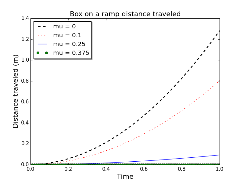
Refer to caption
Figure 9: The distance that the box on the inclined ramp travels over a second for various coefficients of friction.

6.5 Example: stack of spheres

I used the example of stacks of spheres to assess how well the solver scales computationally with numbers of contact constraints. Three constraints (corresponding to ϕn,ϕr,ϕssubscriptitalic-ϕ𝑛subscriptitalic-ϕ𝑟subscriptitalic-ϕ𝑠\phi_{n},\phi_{r},\phi_{s}) were used between each pair of contacting spheres. Although a large number of contacting spheres will generate a large number of optimization variables, the problem is inherently sparse: two contacting spheres yield only a 3×3333\times 3 dense submatrix in the problem Hessian matrix. If each sphere touches at most two others, the ceiling on the total number of nonzero Hessian entries will be 18m18𝑚18m, where m𝑚m is the number of spheres, while the Hessian matrix is expected to be 3m×3m3𝑚3𝑚3m\times 3m, i.e., 9m29superscript𝑚29m^{2} total entries.

The simulation was started with all spheres in mid-air, spaced evenly apart vertically (all spheres are in perfect horizontal alignment), and at rest. As the simulation progresses, the bottom sphere collides with the ground, the second sphere collides with the bottom sphere, etc. Wave propagation effects moving up the stack and due to the various collisions are clearly visible in the accompanying video. The stability of the approach is such that the spheres are able to form a stable stack without any constraints (e.g., walls around the stack) keeping them balanced.

I simulated the stack of spheres using RPI-MATLAB-Simulator for 500 iterations at a step size of 10 ms (selected arbitrarily). I tested stacks of up to 100 spheres, each of which used Young’s Modulus of E=1011N/m2𝐸superscript1011Nsuperscriptm2E=10^{11}\textrm{N}/\textrm{m}^{2} and damping parameter B=INsm𝐵𝐼NsmB=I\frac{\textrm{N}\cdot\textrm{s}}{\textrm{m}}. Performance results are plotted in Figure 10. Although explicit schemes should be capable of simulating stacks of softer spheres much more quickly, we are not aware of a competing approach that can robustly simulate stacks of such stiff spheres nearly as fast (cf. [16], which describes numerous issues with simulating stacks of rigid objects quickly and robustly). Thus, we trade peak performance at simulating contacting rigid bodies over a subset of material properties for good overall performance on arbitrary materials.
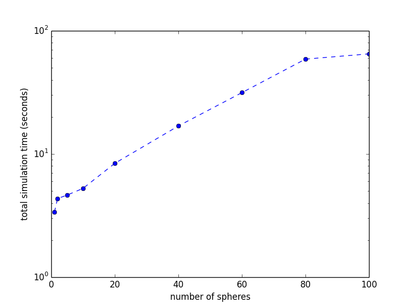
Refer to caption
Figure 10: Times (vertical axis) required to simulate stacks of numbers of spheres (horizontal axis) for one second of virtual time. Each sphere in the stack adds three variables to the convex optimization problem.

7 Discussion

My approach is first-order accurate, assuming that all events are isolated. For simulation, the approach should be competitive (if not much faster) and more numerically robust than approaches that model constraints as rigid: convex optimization problems are far easier to solve than complementarity problems. My method should be faster on many problems than Newton-Raphson-based implicit integrators for simulations than model constraints as springs and dampers; the exception will be those problems that have many more constraints than state variables (like the example in §5, for which my method still exhibited the best worst-case performance compared to state of the art explicit and implicit integrators). And my method has the advantage of being very easy to implement, despite the appearances from the pages of algebra that produced the final simplifications.

This article did not explore applications other than simulation (i.e., control, state estimation, and system identification). Compliant models used in those applications all suffer from the drawback that deformation can be very hard, if not infeasible, to measure particularly when materials are stiff and deformations small. My constraint-based approach seems well suited for these applications because it can estimate forces in the absence of deformation measurements (by treating the deformation as zero) and because it does not suffer from the problems of rigid models. Ultimately, I expect this kind of quasistatic treatment to be reasonable when the constraint acts more plastic than elastic (e.g., like when an object is contacting mud) or when the constraint is very stiff and vibrations dissipate rapidly. I plan to investigate the reasonableness of this quasistatic treatment in future work.

I also plan future investigations that attempt to exploit this constraint solver to do faster and more accurate state estimation, control, and system identification in applications where robots interact with their environments through contact.

Acknowledgements

I thank Dylan Shell, Paul Mitiguy, Hongkai Dai, Ryan Elandt, and Andy Ruina for providing excellent feedback on the manuscript and Michael Sherman for posing early critiques that helped shape its direction.

Appendix 0.A Minimizing variables for all constraints (bilateral, unilateral, and contact constraints in 3D)

This section considers how to minimize all variables for systems with bilateral constraints (variables with subscript b), unilateral constraints (variables with subscript u), and contact constraints in 3D (variables with subscripts n, r, or s). I have included this section to keep the reader from having to do these simplifications. We first formulate the necessary differential optimization problem as a straightforward extension of the techniques presented in Sections 4.2 and 5.3:

minλ,ϕ1,ϕ˙1,βsubscriptmin𝜆subscriptitalic-ϕ1subscript˙italic-ϕ1𝛽\displaystyle\operatorname*{min}_{\lambda,\phi_{1},\dot{\phi}_{1},\beta}\ 12(ζλn1𝖳λn1+ζλu1𝖳λu1+λr1𝖳λr1+βr𝖳βr+λs1𝖳λs1+βs𝖳βs)12𝜁superscriptsubscript𝜆subscript𝑛1𝖳subscript𝜆subscript𝑛1𝜁superscriptsubscript𝜆subscript𝑢1𝖳subscript𝜆subscript𝑢1superscriptsubscript𝜆subscript𝑟1𝖳subscript𝜆subscript𝑟1superscriptsubscript𝛽𝑟𝖳subscript𝛽𝑟superscriptsubscript𝜆subscript𝑠1𝖳subscript𝜆subscript𝑠1superscriptsubscript𝛽𝑠𝖳subscript𝛽𝑠\displaystyle\frac{1}{2}(\zeta{\lambda_{n_{1}}}^{\mathsf{T}}\lambda_{n_{1}}+\zeta{\lambda_{u_{1}}}^{\mathsf{T}}{\lambda_{u_{1}}}+{\lambda_{r_{1}}}^{\mathsf{T}}\lambda_{r_{1}}+{\beta_{r}}^{\mathsf{T}}{\beta_{r}}+{\lambda_{s_{1}}}^{\mathsf{T}}\lambda_{s_{1}}+{\beta_{s}}^{\mathsf{T}}\beta_{s}) (124)
ϕu1subscriptitalic-ϕsubscript𝑢1\displaystyle\phi_{u_{1}} =ϕu0+hϕ˙u1+O(h2)absentsubscriptitalic-ϕsubscript𝑢0subscript˙italic-ϕsubscript𝑢1𝑂superscript2\displaystyle=\phi_{u_{0}}+h\dot{\phi}_{u_{1}}+O(h^{2}) (125)
ϕ˙u1subscript˙italic-ϕsubscript𝑢1\displaystyle\dot{\phi}_{u_{1}} =ϕ˙u0+hϕ¨u0+O(h2)absentsubscript˙italic-ϕsubscript𝑢0subscript¨italic-ϕsubscript𝑢0𝑂superscript2\displaystyle=\dot{\phi}_{u_{0}}+h\ddot{\phi}_{u_{0}}+O(h^{2}) (126)
ϕb1subscriptitalic-ϕsubscript𝑏1\displaystyle\phi_{b_{1}} =ϕb0+hϕ˙b1+O(h2)absentsubscriptitalic-ϕsubscript𝑏0subscript˙italic-ϕsubscript𝑏1𝑂superscript2\displaystyle=\phi_{b_{0}}+h\dot{\phi}_{b_{1}}+O(h^{2}) (127)
ϕ˙b1subscript˙italic-ϕsubscript𝑏1\displaystyle\dot{\phi}_{b_{1}} =ϕ˙b0+hϕ¨b0+O(h2)absentsubscript˙italic-ϕsubscript𝑏0subscript¨italic-ϕsubscript𝑏0𝑂superscript2\displaystyle=\dot{\phi}_{b_{0}}+h\ddot{\phi}_{b_{0}}+O(h^{2}) (128)
ϕn1subscriptitalic-ϕsubscript𝑛1\displaystyle\phi_{n_{1}} =ϕn0+hϕ˙n1+O(h2)absentsubscriptitalic-ϕsubscript𝑛0subscript˙italic-ϕsubscript𝑛1𝑂superscript2\displaystyle=\phi_{n_{0}}+h\dot{\phi}_{n_{1}}+O(h^{2}) (129)
ϕ˙n1subscript˙italic-ϕsubscript𝑛1\displaystyle\dot{\phi}_{n_{1}} =ϕ˙n0+hϕ¨n0+O(h2)absentsubscript˙italic-ϕsubscript𝑛0subscript¨italic-ϕsubscript𝑛0𝑂superscript2\displaystyle=\dot{\phi}_{n_{0}}+h\ddot{\phi}_{n_{0}}+O(h^{2}) (130)
ϕr1subscriptitalic-ϕsubscript𝑟1\displaystyle\phi_{r_{1}} =ϕr0+hϕ˙r1+O(h2)absentsubscriptitalic-ϕsubscript𝑟0subscript˙italic-ϕsubscript𝑟1𝑂superscript2\displaystyle=\phi_{r_{0}}+h\dot{\phi}_{r_{1}}+O(h^{2}) (131)
ϕ˙r1subscript˙italic-ϕsubscript𝑟1\displaystyle\dot{\phi}_{r_{1}} =ϕ˙r0+hϕ¨r0+O(h2)absentsubscript˙italic-ϕsubscript𝑟0subscript¨italic-ϕsubscript𝑟0𝑂superscript2\displaystyle=\dot{\phi}_{r_{0}}+h\ddot{\phi}_{r_{0}}+O(h^{2}) (132)
ϕs1subscriptitalic-ϕsubscript𝑠1\displaystyle\phi_{s_{1}} =ϕs0+hϕ˙s1+O(h2)absentsubscriptitalic-ϕsubscript𝑠0subscript˙italic-ϕsubscript𝑠1𝑂superscript2\displaystyle=\phi_{s_{0}}+h\dot{\phi}_{s_{1}}+O(h^{2}) (133)
ϕ˙s1subscript˙italic-ϕsubscript𝑠1\displaystyle\dot{\phi}_{s_{1}} =ϕ˙s0+hϕ¨s0+O(h2)absentsubscript˙italic-ϕsubscript𝑠0subscript¨italic-ϕsubscript𝑠0𝑂superscript2\displaystyle=\dot{\phi}_{s_{0}}+h\ddot{\phi}_{s_{0}}+O(h^{2}) (134)
λu1subscript𝜆subscript𝑢1\displaystyle\lambda_{u_{1}} Kuϕu1Buϕ˙u1M^uG˙uv0+O(h)absentsubscript𝐾𝑢subscriptitalic-ϕsubscript𝑢1subscript𝐵𝑢subscript˙italic-ϕsubscript𝑢1subscript^𝑀𝑢subscript˙𝐺𝑢subscript𝑣0𝑂\displaystyle\geq-K_{u}\phi_{u_{1}}-B_{u}\dot{\phi}_{u_{1}}-\hat{M}_{u}\dot{G}_{u}v_{0}+O(h) (135)
λu1subscript𝜆subscript𝑢1\displaystyle\lambda_{u_{1}} 0absent0\displaystyle\geq 0 (136)
λn1subscript𝜆subscript𝑛1\displaystyle\lambda_{n_{1}} Knϕn1Bnϕ˙n1M^nG˙nv0+O(h)absentsubscript𝐾𝑛subscriptitalic-ϕsubscript𝑛1subscript𝐵𝑛subscript˙italic-ϕsubscript𝑛1subscript^𝑀𝑛subscript˙𝐺𝑛subscript𝑣0𝑂\displaystyle\geq-K_{n}\phi_{n_{1}}-B_{n}\dot{\phi}_{n_{1}}-\hat{M}_{n}\dot{G}_{n}v_{0}+O(h) (137)
λn1subscript𝜆subscript𝑛1\displaystyle\lambda_{n_{1}} 0absent0\displaystyle\geq 0 (138)
λr1subscript𝜆subscript𝑟1\displaystyle\lambda_{r_{1}} =Krϕr1Brϕ˙r1M^rG˙rv0+βr+O(h)absentsubscript𝐾𝑟subscriptitalic-ϕsubscript𝑟1subscript𝐵𝑟subscript˙italic-ϕsubscript𝑟1subscript^𝑀𝑟subscript˙𝐺𝑟subscript𝑣0subscript𝛽𝑟𝑂\displaystyle=-K_{r}\phi_{r_{1}}-B_{r}\dot{\phi}_{r_{1}}-\hat{M}_{r}\dot{G}_{r}v_{0}+\beta_{r}+O(h) (139)
λs1subscript𝜆subscript𝑠1\displaystyle\lambda_{s_{1}} =Ksϕs1Bsϕ˙s1M^sG˙sv0+βs+O(h)absentsubscript𝐾𝑠subscriptitalic-ϕsubscript𝑠1subscript𝐵𝑠subscript˙italic-ϕsubscript𝑠1subscript^𝑀𝑠subscript˙𝐺𝑠subscript𝑣0subscript𝛽𝑠𝑂\displaystyle=-K_{s}\phi_{s_{1}}-B_{s}\dot{\phi}_{s_{1}}-\hat{M}_{s}\dot{G}_{s}v_{0}+\beta_{s}+O(h) (140)
λb1subscript𝜆subscript𝑏1\displaystyle\lambda_{b_{1}} =Kbϕb1Bbϕ˙b1M^bG˙bv0+O(h)absentsubscript𝐾𝑏subscriptitalic-ϕsubscript𝑏1subscript𝐵𝑏subscript˙italic-ϕsubscript𝑏1subscript^𝑀𝑏subscript˙𝐺𝑏subscript𝑣0𝑂\displaystyle=-K_{b}\phi_{b_{1}}-B_{b}\dot{\phi}_{b_{1}}-\hat{M}_{b}\dot{G}_{b}v_{0}+O(h) (141)
μ2λn12superscript𝜇2superscriptsubscript𝜆subscript𝑛12\displaystyle\mu^{2}\lambda_{n_{1}}^{2} λr12+λs12.absentsuperscriptsubscript𝜆subscript𝑟12superscriptsubscript𝜆subscript𝑠12\displaystyle\geq\lambda_{r_{1}}^{2}+\lambda_{s_{1}}^{2}. (142)

As with the previous section, this section will minimize the number of variables, equation numbers will only be provided when an equation changes, but the whole QP will be reproduced at each step. We first replace all of the ϕ1subscriptitalic-ϕ1\phi_{1} terms: ϕb1,ϕu1,ϕn1,ϕr1, and ϕs1subscriptitalic-ϕsubscript𝑏1subscriptitalic-ϕsubscript𝑢1subscriptitalic-ϕsubscript𝑛1subscriptitalic-ϕsubscript𝑟1 and subscriptitalic-ϕsubscript𝑠1\phi_{b_{1}},\phi_{u_{1}},\phi_{n_{1}},\phi_{r_{1}},\textrm{ and }\phi_{s_{1}}:

minλ,ϕ˙1,βsubscriptmin𝜆subscript˙italic-ϕ1𝛽\displaystyle\operatorname*{min}_{\lambda,\dot{\phi}_{1},\beta}\ 12(ζλn1𝖳λn1+ζλu1𝖳λu1+λr1𝖳λr1+βr𝖳βr+λs1𝖳λs1+βs𝖳βs)12𝜁superscriptsubscript𝜆subscript𝑛1𝖳subscript𝜆subscript𝑛1𝜁superscriptsubscript𝜆subscript𝑢1𝖳subscript𝜆subscript𝑢1superscriptsubscript𝜆subscript𝑟1𝖳subscript𝜆subscript𝑟1superscriptsubscript𝛽𝑟𝖳subscript𝛽𝑟superscriptsubscript𝜆subscript𝑠1𝖳subscript𝜆subscript𝑠1superscriptsubscript𝛽𝑠𝖳subscript𝛽𝑠\displaystyle\frac{1}{2}(\zeta{\lambda_{n_{1}}}^{\mathsf{T}}\lambda_{n_{1}}+\zeta{\lambda_{u_{1}}}^{\mathsf{T}}{\lambda_{u_{1}}}+{\lambda_{r_{1}}}^{\mathsf{T}}\lambda_{r_{1}}+{\beta_{r}}^{\mathsf{T}}{\beta_{r}}+{\lambda_{s_{1}}}^{\mathsf{T}}\lambda_{s_{1}}+{\beta_{s}}^{\mathsf{T}}\beta_{s})
ϕ˙u1subscript˙italic-ϕsubscript𝑢1\displaystyle\dot{\phi}_{u_{1}} =ϕ˙u0+hϕ¨u+O(h2)absentsubscript˙italic-ϕsubscript𝑢0subscript¨italic-ϕ𝑢𝑂superscript2\displaystyle=\dot{\phi}_{u_{0}}+h\ddot{\phi}_{u}+O(h^{2})
ϕ˙b1subscript˙italic-ϕsubscript𝑏1\displaystyle\dot{\phi}_{b_{1}} =ϕ˙b0+hϕ¨b+O(h2)absentsubscript˙italic-ϕsubscript𝑏0subscript¨italic-ϕ𝑏𝑂superscript2\displaystyle=\dot{\phi}_{b_{0}}+h\ddot{\phi}_{b}+O(h^{2})
ϕ˙n1subscript˙italic-ϕsubscript𝑛1\displaystyle\dot{\phi}_{n_{1}} =ϕ˙n0+hϕ¨n+O(h2)absentsubscript˙italic-ϕsubscript𝑛0subscript¨italic-ϕ𝑛𝑂superscript2\displaystyle=\dot{\phi}_{n_{0}}+h\ddot{\phi}_{n}+O(h^{2})
ϕ˙r1subscript˙italic-ϕsubscript𝑟1\displaystyle\dot{\phi}_{r_{1}} =ϕ˙r0+hϕ¨r0+O(h2)absentsubscript˙italic-ϕsubscript𝑟0subscript¨italic-ϕsubscript𝑟0𝑂superscript2\displaystyle=\dot{\phi}_{r_{0}}+h\ddot{\phi}_{r_{0}}+O(h^{2})
ϕ˙s1subscript˙italic-ϕsubscript𝑠1\displaystyle\dot{\phi}_{s_{1}} =ϕ˙s0+hϕ¨s0+O(h2)absentsubscript˙italic-ϕsubscript𝑠0subscript¨italic-ϕsubscript𝑠0𝑂superscript2\displaystyle=\dot{\phi}_{s_{0}}+h\ddot{\phi}_{s_{0}}+O(h^{2})
λu1subscript𝜆subscript𝑢1\displaystyle\lambda_{u_{1}} Kuϕu0(hKu+Bu)ϕ˙u1M^uG˙uv0+O(h)absentsubscript𝐾𝑢subscriptitalic-ϕsubscript𝑢0subscript𝐾𝑢subscript𝐵𝑢subscript˙italic-ϕsubscript𝑢1subscript^𝑀𝑢subscript˙𝐺𝑢subscript𝑣0𝑂\displaystyle\geq-K_{u}\phi_{u_{0}}-(hK_{u}+B_{u})\dot{\phi}_{u_{1}}-\hat{M}_{u}\dot{G}_{u}v_{0}+O(h) (143)
λu1subscript𝜆subscript𝑢1\displaystyle\lambda_{u_{1}} 0absent0\displaystyle\geq 0
λn1subscript𝜆subscript𝑛1\displaystyle\lambda_{n_{1}} Knϕn0(hKn+Bn)ϕ˙n1M^nG˙nv0+O(h)absentsubscript𝐾𝑛subscriptitalic-ϕsubscript𝑛0subscript𝐾𝑛subscript𝐵𝑛subscript˙italic-ϕsubscript𝑛1subscript^𝑀𝑛subscript˙𝐺𝑛subscript𝑣0𝑂\displaystyle\geq-K_{n}\phi_{n_{0}}-(hK_{n}+B_{n})\dot{\phi}_{n_{1}}-\hat{M}_{n}\dot{G}_{n}v_{0}+O(h) (144)
λn1subscript𝜆subscript𝑛1\displaystyle\lambda_{n_{1}} 0absent0\displaystyle\geq 0
λr1subscript𝜆subscript𝑟1\displaystyle\lambda_{r_{1}} =Krϕr0(hKr+Br)ϕ˙r1M^rG˙rv0+βr+O(h)absentsubscript𝐾𝑟subscriptitalic-ϕsubscript𝑟0subscript𝐾𝑟subscript𝐵𝑟subscript˙italic-ϕsubscript𝑟1subscript^𝑀𝑟subscript˙𝐺𝑟subscript𝑣0subscript𝛽𝑟𝑂\displaystyle=-K_{r}\phi_{r_{0}}-(hK_{r}+B_{r})\dot{\phi}_{r_{1}}-\hat{M}_{r}\dot{G}_{r}v_{0}+\beta_{r}+O(h) (145)
λs1subscript𝜆subscript𝑠1\displaystyle\lambda_{s_{1}} =Krϕs0(hKs+Bs)ϕ˙s1M^sG˙sv0+βs+O(h)absentsubscript𝐾𝑟subscriptitalic-ϕsubscript𝑠0subscript𝐾𝑠subscript𝐵𝑠subscript˙italic-ϕsubscript𝑠1subscript^𝑀𝑠subscript˙𝐺𝑠subscript𝑣0subscript𝛽𝑠𝑂\displaystyle=-K_{r}\phi_{s_{0}}-(hK_{s}+B_{s})\dot{\phi}_{s_{1}}-\hat{M}_{s}\dot{G}_{s}v_{0}+\beta_{s}+O(h) (146)
λb1subscript𝜆subscript𝑏1\displaystyle\lambda_{b_{1}} =Kbϕb0(hKb+Bb)ϕ˙b1M^bG˙bv0+O(h)absentsubscript𝐾𝑏subscriptitalic-ϕsubscript𝑏0subscript𝐾𝑏subscript𝐵𝑏subscript˙italic-ϕsubscript𝑏1subscript^𝑀𝑏subscript˙𝐺𝑏subscript𝑣0𝑂\displaystyle=-K_{b}\phi_{b_{0}}-(hK_{b}+B_{b})\dot{\phi}_{b_{1}}-\hat{M}_{b}\dot{G}_{b}v_{0}+O(h) (147)
μ2λn12superscript𝜇2superscriptsubscript𝜆subscript𝑛12\displaystyle\mu^{2}\lambda_{n_{1}}^{2} λr12+λs12.absentsuperscriptsubscript𝜆subscript𝑟12superscriptsubscript𝜆subscript𝑠12\displaystyle\geq\lambda_{r_{1}}^{2}+\lambda_{s_{1}}^{2}.

We then replace all of the ϕ˙1subscript˙italic-ϕ1\dot{\phi}_{1} terms: ϕ˙b1,ϕ˙u1,ϕ˙n1,ϕ˙r1, and ϕ˙s1subscript˙italic-ϕsubscript𝑏1subscript˙italic-ϕsubscript𝑢1subscript˙italic-ϕsubscript𝑛1subscript˙italic-ϕsubscript𝑟1 and subscript˙italic-ϕsubscript𝑠1\dot{\phi}_{b_{1}},\dot{\phi}_{u_{1}},\dot{\phi}_{n_{1}},\dot{\phi}_{r_{1}},\textrm{ and }\dot{\phi}_{s_{1}}:

minλ,ϕ˙1,βsubscriptmin𝜆subscript˙italic-ϕ1𝛽\displaystyle\operatorname*{min}_{\lambda,\dot{\phi}_{1},\beta}\ 12(ζλn1𝖳λn1+ζλu1𝖳λu1+λr1𝖳λr1+βr𝖳βr+λs1𝖳λs1+βs𝖳βs)12𝜁superscriptsubscript𝜆subscript𝑛1𝖳subscript𝜆subscript𝑛1𝜁superscriptsubscript𝜆subscript𝑢1𝖳subscript𝜆subscript𝑢1superscriptsubscript𝜆subscript𝑟1𝖳subscript𝜆subscript𝑟1superscriptsubscript𝛽𝑟𝖳subscript𝛽𝑟superscriptsubscript𝜆subscript𝑠1𝖳subscript𝜆subscript𝑠1superscriptsubscript𝛽𝑠𝖳subscript𝛽𝑠\displaystyle\frac{1}{2}(\zeta{\lambda_{n_{1}}}^{\mathsf{T}}\lambda_{n_{1}}+\zeta{\lambda_{u_{1}}}^{\mathsf{T}}{\lambda_{u_{1}}}+{\lambda_{r_{1}}}^{\mathsf{T}}\lambda_{r_{1}}+{\beta_{r}}^{\mathsf{T}}{\beta_{r}}+{\lambda_{s_{1}}}^{\mathsf{T}}\lambda_{s_{1}}+{\beta_{s}}^{\mathsf{T}}\beta_{s})
λu1subscript𝜆subscript𝑢1\displaystyle\lambda_{u_{1}} Kuϕu0(hKu+Bu)(ϕ˙u0+hϕ¨u+O(h2))ϕ˙u1absentsubscript𝐾𝑢subscriptitalic-ϕsubscript𝑢0subscript𝐾𝑢subscript𝐵𝑢subscriptsubscript˙italic-ϕsubscript𝑢0subscript¨italic-ϕ𝑢𝑂superscript2subscript˙italic-ϕsubscript𝑢1\displaystyle\geq-K_{u}\phi_{u_{0}}-(hK_{u}+B_{u})\underbrace{(\dot{\phi}_{u_{0}}+h\ddot{\phi}_{u}+O(h^{2}))}_{\dot{\phi}_{u_{1}}}-\ldots
M^uG˙uv0+O(h)subscript^𝑀𝑢subscript˙𝐺𝑢subscript𝑣0𝑂\displaystyle\qquad\hat{M}_{u}\dot{G}_{u}v_{0}+O(h) (148)
λu1subscript𝜆subscript𝑢1\displaystyle\lambda_{u_{1}} 0absent0\displaystyle\geq 0
λn1subscript𝜆subscript𝑛1\displaystyle\lambda_{n_{1}} Knϕn0(hKn+Bn)(ϕ˙n0+hϕ¨n+O(h2))ϕ˙n1absentsubscript𝐾𝑛subscriptitalic-ϕsubscript𝑛0subscript𝐾𝑛subscript𝐵𝑛subscriptsubscript˙italic-ϕsubscript𝑛0subscript¨italic-ϕ𝑛𝑂superscript2subscript˙italic-ϕsubscript𝑛1\displaystyle\geq-K_{n}\phi_{n_{0}}-(hK_{n}+B_{n})\underbrace{(\dot{\phi}_{n_{0}}+h\ddot{\phi}_{n}+O(h^{2}))}_{\dot{\phi}_{n_{1}}}-\ldots
M^nG˙nv0+O(h)subscript^𝑀𝑛subscript˙𝐺𝑛subscript𝑣0𝑂\displaystyle\qquad\hat{M}_{n}\dot{G}_{n}v_{0}+O(h) (149)
λn1subscript𝜆subscript𝑛1\displaystyle\lambda_{n_{1}} 0absent0\displaystyle\geq 0
λr1subscript𝜆subscript𝑟1\displaystyle\lambda_{r_{1}} =Krϕr0(hKr+Br)(ϕ˙r0+hϕ¨r0+O(h2))ϕ˙r1absentsubscript𝐾𝑟subscriptitalic-ϕsubscript𝑟0subscript𝐾𝑟subscript𝐵𝑟subscriptsubscript˙italic-ϕsubscript𝑟0subscript¨italic-ϕsubscript𝑟0𝑂superscript2subscript˙italic-ϕsubscript𝑟1\displaystyle=-K_{r}\phi_{r_{0}}-(hK_{r}+B_{r})\underbrace{(\dot{\phi}_{r_{0}}+h\ddot{\phi}_{r_{0}}+O(h^{2}))}_{\dot{\phi}_{r_{1}}}-\ldots
M^rG˙rv0+βr+O(h)subscript^𝑀𝑟subscript˙𝐺𝑟subscript𝑣0subscript𝛽𝑟𝑂\displaystyle\qquad\hat{M}_{r}\dot{G}_{r}v_{0}+\beta_{r}+O(h) (150)
λs1subscript𝜆subscript𝑠1\displaystyle\lambda_{s_{1}} =Krϕs0(hKs+Bs)(ϕ˙s0+hϕ¨s0+O(h2))ϕ˙s1absentsubscript𝐾𝑟subscriptitalic-ϕsubscript𝑠0subscript𝐾𝑠subscript𝐵𝑠subscriptsubscript˙italic-ϕsubscript𝑠0subscript¨italic-ϕsubscript𝑠0𝑂superscript2subscript˙italic-ϕsubscript𝑠1\displaystyle=-K_{r}\phi_{s_{0}}-(hK_{s}+B_{s})\underbrace{(\dot{\phi}_{s_{0}}+h\ddot{\phi}_{s_{0}}+O(h^{2}))}_{\dot{\phi}_{s_{1}}}-\ldots
M^sG˙sv0+βs+O(h)subscript^𝑀𝑠subscript˙𝐺𝑠subscript𝑣0subscript𝛽𝑠𝑂\displaystyle\qquad\hat{M}_{s}\dot{G}_{s}v_{0}+\beta_{s}+O(h) (151)
λb1subscript𝜆subscript𝑏1\displaystyle\lambda_{b_{1}} =Kbϕb0(hKb+Bb)(ϕ˙b0+hϕ¨b+O(h2))ϕ˙b1absentsubscript𝐾𝑏subscriptitalic-ϕsubscript𝑏0subscript𝐾𝑏subscript𝐵𝑏subscriptsubscript˙italic-ϕsubscript𝑏0subscript¨italic-ϕ𝑏𝑂superscript2subscript˙italic-ϕsubscript𝑏1\displaystyle=-K_{b}\phi_{b_{0}}-(hK_{b}+B_{b})\underbrace{(\dot{\phi}_{b_{0}}+h\ddot{\phi}_{b}+O(h^{2}))}_{\dot{\phi}_{b_{1}}}-\ldots
M^bG˙bv0+O(h)subscript^𝑀𝑏subscript˙𝐺𝑏subscript𝑣0𝑂\displaystyle\qquad\hat{M}_{b}\dot{G}_{b}v_{0}+O(h) (152)
μ2λn12superscript𝜇2superscriptsubscript𝜆subscript𝑛12\displaystyle\mu^{2}\lambda_{n_{1}}^{2} λr12+λs12.absentsuperscriptsubscript𝜆subscript𝑟12superscriptsubscript𝜆subscript𝑠12\displaystyle\geq\lambda_{r_{1}}^{2}+\lambda_{s_{1}}^{2}.

As demonstrated many times previously, the hO(h2)𝑂superscript2hO(h^{2}) terms are subsumed by the O(h)𝑂O(h) terms, so we make that simplification and also leverage the identities v˙0=M𝟣(Gn𝖳λn1+Gr𝖳λr1+Gs𝖳λs1+Gu𝖳λu1+Gb𝖳λb1+f)+O(h)subscript˙𝑣0superscript𝑀1superscriptsubscript𝐺𝑛𝖳subscript𝜆subscript𝑛1superscriptsubscript𝐺𝑟𝖳subscript𝜆subscript𝑟1superscriptsubscript𝐺𝑠𝖳subscript𝜆subscript𝑠1superscriptsubscript𝐺𝑢𝖳subscript𝜆subscript𝑢1superscriptsubscript𝐺𝑏𝖳subscript𝜆subscript𝑏1𝑓𝑂\dot{v}_{0}={M}^{\mathsf{-1}}({G_{n}}^{\mathsf{T}}\lambda_{n_{1}}+{G_{r}}^{\mathsf{T}}\lambda_{r_{1}}+{G_{s}}^{\mathsf{T}}\lambda_{s_{1}}+{G_{u}}^{\mathsf{T}}\lambda_{u_{1}}+{G_{b}}^{\mathsf{T}}\lambda_{b_{1}}+f)+O(h), ϕ¨n0=Gnv˙0+G˙nv0subscript¨italic-ϕsubscript𝑛0subscript𝐺𝑛subscript˙𝑣0subscript˙𝐺𝑛subscript𝑣0\ddot{\phi}_{n_{0}}=G_{n}\dot{v}_{0}+\dot{G}_{n}v_{0}, ϕ¨r0=Grv˙0+G˙rv0subscript¨italic-ϕsubscript𝑟0subscript𝐺𝑟subscript˙𝑣0subscript˙𝐺𝑟subscript𝑣0\ddot{\phi}_{r_{0}}=G_{r}\dot{v}_{0}+\dot{G}_{r}v_{0}, ϕ¨s0=Gsv˙0+G˙sv0subscript¨italic-ϕsubscript𝑠0subscript𝐺𝑠subscript˙𝑣0subscript˙𝐺𝑠subscript𝑣0\ddot{\phi}_{s_{0}}=G_{s}\dot{v}_{0}+\dot{G}_{s}v_{0}, ϕ¨u0=Guv˙0+G˙uv0subscript¨italic-ϕsubscript𝑢0subscript𝐺𝑢subscript˙𝑣0subscript˙𝐺𝑢subscript𝑣0\ddot{\phi}_{u_{0}}=G_{u}\dot{v}_{0}+\dot{G}_{u}v_{0}, ϕ¨u0=Guv˙0+G˙uv0subscript¨italic-ϕsubscript𝑢0subscript𝐺𝑢subscript˙𝑣0subscript˙𝐺𝑢subscript𝑣0\ddot{\phi}_{u_{0}}=G_{u}\dot{v}_{0}+\dot{G}_{u}v_{0}, and ϕ¨b0=Gbv˙0+G˙bv0subscript¨italic-ϕsubscript𝑏0subscript𝐺𝑏subscript˙𝑣0subscript˙𝐺𝑏subscript𝑣0\ddot{\phi}_{b_{0}}=G_{b}\dot{v}_{0}+\dot{G}_{b}v_{0}:

minλ,βsubscriptmin𝜆𝛽\displaystyle\operatorname*{min}_{\lambda,\beta}\ 12(ζλn1𝖳λn1+ζλu1𝖳λu1+λr1𝖳λr1+βr𝖳βr+βs𝖳βs)12𝜁superscriptsubscript𝜆subscript𝑛1𝖳subscript𝜆subscript𝑛1𝜁superscriptsubscript𝜆subscript𝑢1𝖳subscript𝜆subscript𝑢1superscriptsubscript𝜆subscript𝑟1𝖳subscript𝜆subscript𝑟1superscriptsubscript𝛽𝑟𝖳subscript𝛽𝑟superscriptsubscript𝛽𝑠𝖳subscript𝛽𝑠\displaystyle\frac{1}{2}(\zeta{\lambda_{n_{1}}}^{\mathsf{T}}\lambda_{n_{1}}+\zeta{\lambda_{u_{1}}}^{\mathsf{T}}{\lambda_{u_{1}}}+{\lambda_{r_{1}}}^{\mathsf{T}}\lambda_{r_{1}}+{\beta_{r}}^{\mathsf{T}}{\beta_{r}}+{\beta_{s}}^{\mathsf{T}}{\beta_{s}})
λu1subscript𝜆subscript𝑢1\displaystyle\lambda_{u_{1}} M^uG˙uv0Kuϕu0(hKu+Bu)(ϕ˙u0+h\displaystyle\geq-\hat{M}_{u}\dot{G}_{u}v_{0}-K_{u}\phi_{u_{0}}-(hK_{u}+B_{u})(\dot{\phi}_{u_{0}}+h\ldots
(GuM𝟣(Gn𝖳λn1+Gr𝖳λr1+Gs𝖳λs1+Gu𝖳λu1+Gb𝖳λb1+f)+G˙uv0)ϕ¨u0)\displaystyle\underbrace{(G_{u}{M}^{\mathsf{-1}}({G_{n}}^{\mathsf{T}}\lambda_{n_{1}}+{G_{r}}^{\mathsf{T}}\lambda_{r_{1}}+{G_{s}}^{\mathsf{T}}\lambda_{s_{1}}+{G_{u}}^{\mathsf{T}}\lambda_{u_{1}}+{G_{b}}^{\mathsf{T}}\lambda_{b_{1}}+f)+\dot{G}_{u}v_{0})}_{\ddot{\phi}_{u_{0}}}) (153)
λu1subscript𝜆subscript𝑢1\displaystyle\lambda_{u_{1}} 0absent0\displaystyle\geq 0
λn1subscript𝜆subscript𝑛1\displaystyle\lambda_{n_{1}} M^nG˙nv0Knϕn0(hKn+Bn)(ϕ˙n0+h\displaystyle\geq-\hat{M}_{n}\dot{G}_{n}v_{0}-K_{n}\phi_{n_{0}}-(hK_{n}+B_{n})(\dot{\phi}_{n_{0}}+h\ldots
(GnM𝟣(Gn𝖳λn1+Gr𝖳λr1+Gs𝖳λs1+Gu𝖳λu1+Gb𝖳λb1+f)+G˙nv0)ϕ¨n0)\displaystyle\underbrace{(G_{n}{M}^{\mathsf{-1}}({G_{n}}^{\mathsf{T}}\lambda_{n_{1}}+{G_{r}}^{\mathsf{T}}\lambda_{r_{1}}+{G_{s}}^{\mathsf{T}}\lambda_{s_{1}}+{G_{u}}^{\mathsf{T}}\lambda_{u_{1}}+{G_{b}}^{\mathsf{T}}\lambda_{b_{1}}+f)+\dot{G}_{n}v_{0})}_{\ddot{\phi}_{n_{0}}}) (154)
λn1subscript𝜆subscript𝑛1\displaystyle\lambda_{n_{1}} 0absent0\displaystyle\geq 0
λr1subscript𝜆subscript𝑟1\displaystyle\lambda_{r_{1}} =βrM^rG˙rv0Krϕr0(hKr+Br)(ϕ˙r0+h\displaystyle=\beta_{r}-\hat{M}_{r}\dot{G}_{r}v_{0}-K_{r}\phi_{r_{0}}-(hK_{r}+B_{r})(\dot{\phi}_{r_{0}}+h\ldots
(GrM𝟣(Gn𝖳λn1+Gr𝖳λr1+Gs𝖳λs1+Gu𝖳λu1+Gb𝖳λb1+f)+G˙rv0)ϕ¨r0)\displaystyle\underbrace{(G_{r}{M}^{\mathsf{-1}}({G_{n}}^{\mathsf{T}}\lambda_{n_{1}}+{G_{r}}^{\mathsf{T}}\lambda_{r_{1}}+{G_{s}}^{\mathsf{T}}\lambda_{s_{1}}+{G_{u}}^{\mathsf{T}}\lambda_{u_{1}}+{G_{b}}^{\mathsf{T}}\lambda_{b_{1}}+f)+\dot{G}_{r}v_{0})}_{\ddot{\phi}_{r_{0}}}) (155)
λs1subscript𝜆subscript𝑠1\displaystyle\lambda_{s_{1}} =βsM^sG˙sv0Ksϕs0(hKs+Bs)(ϕ˙s0+h\displaystyle=\beta_{s}-\hat{M}_{s}\dot{G}_{s}v_{0}-K_{s}\phi_{s_{0}}-(hK_{s}+B_{s})(\dot{\phi}_{s_{0}}+h\ldots
(GsM𝟣(Gn𝖳λn1+Gr𝖳λr1+Gs𝖳λs1+Gu𝖳λu1+Gb𝖳λb1+f)+G˙rv0)ϕ¨s0)\displaystyle\underbrace{(G_{s}{M}^{\mathsf{-1}}({G_{n}}^{\mathsf{T}}\lambda_{n_{1}}+{G_{r}}^{\mathsf{T}}\lambda_{r_{1}}+{G_{s}}^{\mathsf{T}}\lambda_{s_{1}}+{G_{u}}^{\mathsf{T}}\lambda_{u_{1}}+{G_{b}}^{\mathsf{T}}\lambda_{b_{1}}+f)+\dot{G}_{r}v_{0})}_{\ddot{\phi}_{s_{0}}}) (156)
λb1subscript𝜆subscript𝑏1\displaystyle\lambda_{b_{1}} =M^bG˙bv0Kbϕb0(hKb+Bb)(ϕ˙b0+h\displaystyle=-\hat{M}_{b}\dot{G}_{b}v_{0}-K_{b}\phi_{b_{0}}-(hK_{b}+B_{b})(\dot{\phi}_{b_{0}}+h\ldots
(GbM𝟣(Gn𝖳λn1+Gr𝖳λr1+Gs𝖳λs1+Gu𝖳λu1+Gb𝖳λb1+f)+G˙bv0)ϕ¨b0)\displaystyle\underbrace{(G_{b}{M}^{\mathsf{-1}}({G_{n}}^{\mathsf{T}}\lambda_{n_{1}}+{G_{r}}^{\mathsf{T}}\lambda_{r_{1}}+{G_{s}}^{\mathsf{T}}\lambda_{s_{1}}+{G_{u}}^{\mathsf{T}}\lambda_{u_{1}}+{G_{b}}^{\mathsf{T}}\lambda_{b_{1}}+f)+\dot{G}_{b}v_{0})}_{\ddot{\phi}_{b_{0}}}) (157)
μ2λn12superscript𝜇2superscriptsubscript𝜆subscript𝑛12\displaystyle\mu^{2}\lambda_{n_{1}}^{2} λr12+λs12.absentsuperscriptsubscript𝜆subscript𝑟12superscriptsubscript𝜆subscript𝑠12\displaystyle\geq\lambda_{r_{1}}^{2}+\lambda_{s_{1}}^{2}.

Next, we replace the λb1subscript𝜆subscript𝑏1\lambda_{b_{1}} term by first using the identity M^b(GbM𝟣Gb𝖳)𝟣subscript^𝑀𝑏superscriptsubscript𝐺𝑏superscript𝑀1superscriptsubscript𝐺𝑏𝖳1\hat{M}_{b}\equiv{(G_{b}{M}^{\mathsf{-1}}{G_{b}}^{\mathsf{T}})}^{\mathsf{-1}} and then rearranging (157) to:

(I+(h2Kb+hBb)M^b0𝟣)λb1=𝐼superscript2subscript𝐾𝑏subscript𝐵𝑏superscriptsubscript^𝑀subscript𝑏01subscript𝜆subscript𝑏1absent\displaystyle(I+(h^{2}K_{b}+hB_{b}){\hat{M}_{b_{0}}}^{\mathsf{-1}})\lambda_{b_{1}}= M^uG˙uv0Kbϕb0(hKb+Bb)(\displaystyle\ -\hat{M}_{u}\dot{G}_{u}v_{0}-K_{b}\phi_{b_{0}}-(hK_{b}+B_{b})(\ldots
ϕ˙b0+h(GbM𝟣(Gn𝖳λn1+Gr𝖳λr1+\displaystyle\qquad\dot{\phi}_{b_{0}}+h(G_{b}{M}^{\mathsf{-1}}({G_{n}}^{\mathsf{T}}\lambda_{n_{1}}+{G_{r}}^{\mathsf{T}}\lambda_{r_{1}}+\ldots
Gs𝖳λs1+Gu𝖳λu1+f)+\displaystyle\qquad{G_{s}}^{\mathsf{T}}\lambda_{s_{1}}+{G_{u}}^{\mathsf{T}}\lambda_{u_{1}}+f)+\ldots
G˙bv0))+O(h),\displaystyle\qquad\dot{G}_{b}v_{0}))+O(h), (158)

then defining

c𝑐absent\displaystyle c\equiv M^uG˙uv0Kbϕb0(hKb+Bb)(ϕ˙b0+h(GbM𝟣f+G˙bv0)\displaystyle\ -\hat{M}_{u}\dot{G}_{u}v_{0}-K_{b}\phi_{b_{0}}-(hK_{b}+B_{b})(\dot{\phi}_{b_{0}}+h(G_{b}{M}^{\mathsf{-1}}f+\dot{G}_{b}v_{0}) (159)
D𝐷absent\displaystyle D\equiv (h2Kb+hBb)GbM𝟣superscript2subscript𝐾𝑏subscript𝐵𝑏subscript𝐺𝑏superscript𝑀1\displaystyle\ -(h^{2}K_{b}+hB_{b})G_{b}{M}^{\mathsf{-1}} (160)
C𝐶absent\displaystyle C\equiv (IDGb𝖳)𝐼𝐷superscriptsubscript𝐺𝑏𝖳\displaystyle\ (I-D{G_{b}}^{\mathsf{T}}) (161)
Gsuperscript𝐺absent\displaystyle G^{*}\equiv [Gn𝖳Gr𝖳Gs𝖳Gu𝖳]𝖳superscriptmatrixsuperscriptsubscript𝐺𝑛𝖳superscriptsubscript𝐺𝑟𝖳superscriptsubscript𝐺𝑠𝖳superscriptsubscript𝐺𝑢𝖳𝖳\displaystyle\ {\begin{bmatrix}{G_{n}}^{\mathsf{T}}&{G_{r}}^{\mathsf{T}}&{G_{s}}^{\mathsf{T}}&{G_{u}}^{\mathsf{T}}\end{bmatrix}}^{\mathsf{T}} (162)
λ1subscriptsuperscript𝜆1absent\displaystyle\lambda^{*}_{1}\equiv [λn1𝖳λr1𝖳λs1𝖳λu1𝖳]𝖳,superscriptmatrixsuperscriptsubscript𝜆subscript𝑛1𝖳superscriptsubscript𝜆subscript𝑟1𝖳superscriptsubscript𝜆subscript𝑠1𝖳superscriptsubscript𝜆subscript𝑢1𝖳𝖳\displaystyle\ {\begin{bmatrix}{\lambda_{n_{1}}}^{\mathsf{T}}&{\lambda_{r_{1}}}^{\mathsf{T}}&{\lambda_{s_{1}}}^{\mathsf{T}}&{\lambda_{u_{1}}}^{\mathsf{T}}\end{bmatrix}}^{\mathsf{T}}, (163)

allowing us to reformulate (158) into Cλb1=c+DG𝖳λ1+O(h)𝐶subscript𝜆subscript𝑏1𝑐𝐷superscriptsuperscript𝐺𝖳subscriptsuperscript𝜆1𝑂C\lambda_{b_{1}}=c+D{G^{*}}^{\mathsf{T}}\lambda^{*}_{1}+O(h) or, equivalently, λb1=C𝟣(c+DG𝖳λ1)+O(h)subscript𝜆subscript𝑏1superscript𝐶1𝑐𝐷superscriptsuperscript𝐺𝖳subscriptsuperscript𝜆1𝑂\lambda_{b_{1}}={C}^{\mathsf{-1}}(c+D{G^{*}}^{\mathsf{T}}\lambda^{*}_{1})+O(h). Using this latter relationship, we can replace λb1subscript𝜆subscript𝑏1\lambda_{b_{1}}:

minλ,βsubscriptmin𝜆𝛽\displaystyle\operatorname*{min}_{\lambda,\beta}\ 12(ζλn1𝖳λn1+ζλu1𝖳λu1+λr1𝖳λr1+βr𝖳βr+βs𝖳βs)12𝜁superscriptsubscript𝜆subscript𝑛1𝖳subscript𝜆subscript𝑛1𝜁superscriptsubscript𝜆subscript𝑢1𝖳subscript𝜆subscript𝑢1superscriptsubscript𝜆subscript𝑟1𝖳subscript𝜆subscript𝑟1superscriptsubscript𝛽𝑟𝖳subscript𝛽𝑟superscriptsubscript𝛽𝑠𝖳subscript𝛽𝑠\displaystyle\frac{1}{2}(\zeta{\lambda_{n_{1}}}^{\mathsf{T}}\lambda_{n_{1}}+\zeta{\lambda_{u_{1}}}^{\mathsf{T}}{\lambda_{u_{1}}}+{\lambda_{r_{1}}}^{\mathsf{T}}\lambda_{r_{1}}+{\beta_{r}}^{\mathsf{T}}{\beta_{r}}+{\beta_{s}}^{\mathsf{T}}\beta_{s})
λu1subscript𝜆subscript𝑢1\displaystyle\lambda_{u_{1}} M^uG˙uv0Kuϕu0(hKu+Bu)(ϕ˙u0+h(GuM𝟣(Gn𝖳λn1+\displaystyle\geq-\hat{M}_{u}\dot{G}_{u}v_{0}-K_{u}\phi_{u_{0}}-(hK_{u}+B_{u})(\dot{\phi}_{u_{0}}+h(G_{u}{M}^{\mathsf{-1}}({G_{n}}^{\mathsf{T}}\lambda_{n_{1}}+\ldots
Gr𝖳λr1+Gs𝖳λs1+Gu𝖳λu1+Gb𝖳C𝟣(c+DG𝖳λ1+O(h))λb1+f)+\displaystyle\quad{G_{r}}^{\mathsf{T}}\lambda_{r_{1}}+{G_{s}}^{\mathsf{T}}\lambda_{s_{1}}+{G_{u}}^{\mathsf{T}}\lambda_{u_{1}}+{G_{b}}^{\mathsf{T}}\underbrace{{C}^{\mathsf{-1}}(c+D{G^{*}}^{\mathsf{T}}\lambda^{*}_{1}+O(h))}_{\lambda_{b_{1}}}+f)+\ldots
G˙uv0))+O(h)\displaystyle\quad\dot{G}_{u}v_{0}))+O(h) (164)
λu1subscript𝜆subscript𝑢1\displaystyle\lambda_{u_{1}} 0absent0\displaystyle\geq 0
λn1subscript𝜆subscript𝑛1\displaystyle\lambda_{n_{1}} M^nG˙nv0Knϕn0(hKn+Bn)(ϕ˙n0+h(GnM𝟣(Gn𝖳λn1+\displaystyle\geq-\hat{M}_{n}\dot{G}_{n}v_{0}-K_{n}\phi_{n_{0}}-(hK_{n}+B_{n})(\dot{\phi}_{n_{0}}+h(G_{n}{M}^{\mathsf{-1}}({G_{n}}^{\mathsf{T}}\lambda_{n_{1}}+\ldots
Gr𝖳λr1+Gs𝖳λs1+Gu𝖳λu1+Gb𝖳C𝟣(c+DG𝖳λ1+O(h))λb1+f)+\displaystyle\quad{G_{r}}^{\mathsf{T}}\lambda_{r_{1}}+{G_{s}}^{\mathsf{T}}\lambda_{s_{1}}+{G_{u}}^{\mathsf{T}}\lambda_{u_{1}}+{G_{b}}^{\mathsf{T}}\underbrace{{C}^{\mathsf{-1}}(c+D{G^{*}}^{\mathsf{T}}\lambda^{*}_{1}+O(h))}_{\lambda_{b_{1}}}+f)+\ldots
G˙nv0))+O(h)\displaystyle\quad\dot{G}_{n}v_{0}))+O(h) (165)
λn1subscript𝜆subscript𝑛1\displaystyle\lambda_{n_{1}} 0absent0\displaystyle\geq 0
λr1subscript𝜆subscript𝑟1\displaystyle\lambda_{r_{1}} =M^rG˙rv0Krϕr0(hKr+Br)(ϕ˙r0+h(GrM𝟣(Gn𝖳λn1+\displaystyle=-\hat{M}_{r}\dot{G}_{r}v_{0}-K_{r}\phi_{r_{0}}-(hK_{r}+B_{r})(\dot{\phi}_{r_{0}}+h(G_{r}{M}^{\mathsf{-1}}({G_{n}}^{\mathsf{T}}\lambda_{n_{1}}+\ldots
Gr𝖳λr1+Gs𝖳λs1+Gu𝖳λu1+Gb𝖳C𝟣(c+DG𝖳λ1+O(h))λb1+f)+\displaystyle\quad{G_{r}}^{\mathsf{T}}\lambda_{r_{1}}+{G_{s}}^{\mathsf{T}}\lambda_{s_{1}}+{G_{u}}^{\mathsf{T}}\lambda_{u_{1}}+{G_{b}}^{\mathsf{T}}\underbrace{{C}^{\mathsf{-1}}(c+D{G^{*}}^{\mathsf{T}}\lambda^{*}_{1}+O(h))}_{\lambda_{b_{1}}}+f)+\ldots
G˙rv0))+βr+O(h)\displaystyle\quad\dot{G}_{r}v_{0}))+\beta_{r}+O(h) (166)
λs1subscript𝜆subscript𝑠1\displaystyle\lambda_{s_{1}} =M^sG˙sv0Ksϕs0(hKs+Bs)(ϕ˙s0+h(GsM𝟣(Gn𝖳λn1+\displaystyle=-\hat{M}_{s}\dot{G}_{s}v_{0}-K_{s}\phi_{s_{0}}-(hK_{s}+B_{s})(\dot{\phi}_{s_{0}}+h(G_{s}{M}^{\mathsf{-1}}({G_{n}}^{\mathsf{T}}\lambda_{n_{1}}+\ldots
Gr𝖳λr1+Gs𝖳λs1+Gu𝖳λu1+Gb𝖳C𝟣(c+DG𝖳λ1+O(h))λb1+f)+\displaystyle\quad{G_{r}}^{\mathsf{T}}\lambda_{r_{1}}+{G_{s}}^{\mathsf{T}}\lambda_{s_{1}}+{G_{u}}^{\mathsf{T}}\lambda_{u_{1}}+{G_{b}}^{\mathsf{T}}\underbrace{{C}^{\mathsf{-1}}(c+D{G^{*}}^{\mathsf{T}}\lambda^{*}_{1}+O(h))}_{\lambda_{b_{1}}}+f)+\ldots
G˙sv0))+βs+O(h)\displaystyle\quad\dot{G}_{s}v_{0}))+\beta_{s}+O(h) (167)
μ2λn12superscript𝜇2superscriptsubscript𝜆subscript𝑛12\displaystyle\mu^{2}\lambda_{n_{1}}^{2} λr12+λs12.absentsuperscriptsubscript𝜆subscript𝑟12superscriptsubscript𝜆subscript𝑠12\displaystyle\geq\lambda_{r_{1}}^{2}+\lambda_{s_{1}}^{2}.

We will now remove the subsumed hO(h)𝑂hO(h) terms and the λ1subscriptsuperscript𝜆1\lambda^{*}_{1} terms, replacing the latter with the expansion λ1=[λn1𝖳λr1𝖳λs1𝖳λu1𝖳]𝖳subscriptsuperscript𝜆1superscriptmatrixsuperscriptsubscript𝜆subscript𝑛1𝖳superscriptsubscript𝜆subscript𝑟1𝖳superscriptsubscript𝜆subscript𝑠1𝖳superscriptsubscript𝜆subscript𝑢1𝖳𝖳\lambda^{*}_{1}={\begin{bmatrix}{\lambda_{n_{1}}}^{\mathsf{T}}&{\lambda_{r_{1}}}^{\mathsf{T}}&{\lambda_{s_{1}}}^{\mathsf{T}}&{\lambda_{u_{1}}}^{\mathsf{T}}\end{bmatrix}}^{\mathsf{T}} temporarily (they will be reintroduced for compactness later).

minλ,βsubscriptmin𝜆𝛽\displaystyle\operatorname*{min}_{\lambda,\beta}\ 12(ζλn1𝖳λn1+ζλu1𝖳λu1+λr1𝖳λr1+βr𝖳βr+βs𝖳βs)12𝜁superscriptsubscript𝜆subscript𝑛1𝖳subscript𝜆subscript𝑛1𝜁superscriptsubscript𝜆subscript𝑢1𝖳subscript𝜆subscript𝑢1superscriptsubscript𝜆subscript𝑟1𝖳subscript𝜆subscript𝑟1superscriptsubscript𝛽𝑟𝖳subscript𝛽𝑟superscriptsubscript𝛽𝑠𝖳subscript𝛽𝑠\displaystyle\frac{1}{2}(\zeta{\lambda_{n_{1}}}^{\mathsf{T}}\lambda_{n_{1}}+\zeta{\lambda_{u_{1}}}^{\mathsf{T}}{\lambda_{u_{1}}}+{\lambda_{r_{1}}}^{\mathsf{T}}\lambda_{r_{1}}+{\beta_{r}}^{\mathsf{T}}{\beta_{r}}+{\beta_{s}}^{\mathsf{T}}\beta_{s})
λu1subscript𝜆subscript𝑢1\displaystyle\lambda_{u_{1}} M^uG˙uv0Kuϕu0(hKu+Bu)(ϕ˙u0+h(GuM𝟣(Gb𝖳C𝟣D+I)(\displaystyle\geq-\hat{M}_{u}\dot{G}_{u}v_{0}-K_{u}\phi_{u_{0}}-(hK_{u}+B_{u})(\dot{\phi}_{u_{0}}+h(G_{u}{M}^{\mathsf{-1}}({G_{b}}^{\mathsf{T}}{C}^{\mathsf{-1}}D+I)(\ldots
Gn𝖳λn1+Gr𝖳λr1+Gs𝖳λs1+Gu𝖳λu1+Gb𝖳C𝟣c+f)+\displaystyle\qquad{G_{n}}^{\mathsf{T}}\lambda_{n_{1}}+{G_{r}}^{\mathsf{T}}\lambda_{r_{1}}+{G_{s}}^{\mathsf{T}}\lambda_{s_{1}}+{G_{u}}^{\mathsf{T}}\lambda_{u_{1}}+{G_{b}}^{\mathsf{T}}{C}^{\mathsf{-1}}c+f)+\ldots
G˙uv0))+O(h)\displaystyle\qquad\dot{G}_{u}v_{0}))+O(h) (168)
λu1subscript𝜆subscript𝑢1\displaystyle\lambda_{u_{1}} 0absent0\displaystyle\geq 0
λn1subscript𝜆subscript𝑛1\displaystyle\lambda_{n_{1}} M^nG˙nv0Knϕn0(hKn+Bn)(ϕ˙n0+h(GnM𝟣(Gb𝖳C𝟣D+I)(\displaystyle\geq-\hat{M}_{n}\dot{G}_{n}v_{0}-K_{n}\phi_{n_{0}}-(hK_{n}+B_{n})(\dot{\phi}_{n_{0}}+h(G_{n}{M}^{\mathsf{-1}}({G_{b}}^{\mathsf{T}}{C}^{\mathsf{-1}}D+I)(\ldots
Gn𝖳λn1+Gr𝖳λr1+Gs𝖳λs1+Gu𝖳λu1+Gb𝖳C𝟣c+f)+\displaystyle\qquad{G_{n}}^{\mathsf{T}}\lambda_{n_{1}}+{G_{r}}^{\mathsf{T}}\lambda_{r_{1}}+{G_{s}}^{\mathsf{T}}\lambda_{s_{1}}+{G_{u}}^{\mathsf{T}}\lambda_{u_{1}}+{G_{b}}^{\mathsf{T}}{C}^{\mathsf{-1}}c+f)+\ldots
G˙nv0))+O(h)\displaystyle\qquad\dot{G}_{n}v_{0}))+O(h) (169)
λn1subscript𝜆subscript𝑛1\displaystyle\lambda_{n_{1}} 0absent0\displaystyle\geq 0
λr1subscript𝜆subscript𝑟1\displaystyle\lambda_{r_{1}} =M^rG˙rv0Krϕr0(hKr+Br)(ϕ˙r0+h(GrM𝟣(Gb𝖳C𝟣D+I)(\displaystyle=-\hat{M}_{r}\dot{G}_{r}v_{0}-K_{r}\phi_{r_{0}}-(hK_{r}+B_{r})(\dot{\phi}_{r_{0}}+h(G_{r}{M}^{\mathsf{-1}}({G_{b}}^{\mathsf{T}}{C}^{\mathsf{-1}}D+I)(\ldots
Gn𝖳λn1+Gr𝖳λr1+Gs𝖳λs1+Gu𝖳λu1+Gb𝖳C𝟣c+f)+\displaystyle\qquad{G_{n}}^{\mathsf{T}}\lambda_{n_{1}}+{G_{r}}^{\mathsf{T}}\lambda_{r_{1}}+{G_{s}}^{\mathsf{T}}\lambda_{s_{1}}+{G_{u}}^{\mathsf{T}}\lambda_{u_{1}}+{G_{b}}^{\mathsf{T}}{C}^{\mathsf{-1}}c+f)+\ldots
G˙rv0))+βr+O(h)\displaystyle\qquad\dot{G}_{r}v_{0}))+\beta_{r}+O(h) (170)
λs1subscript𝜆subscript𝑠1\displaystyle\lambda_{s_{1}} =M^sG˙sv0Ksϕs0(hKs+Bs)(ϕ˙s0+h(GsM𝟣(Gb𝖳C𝟣D+I)(\displaystyle=-\hat{M}_{s}\dot{G}_{s}v_{0}-K_{s}\phi_{s_{0}}-(hK_{s}+B_{s})(\dot{\phi}_{s_{0}}+h(G_{s}{M}^{\mathsf{-1}}({G_{b}}^{\mathsf{T}}{C}^{\mathsf{-1}}D+I)(\ldots
Gn𝖳λn1+Gr𝖳λr1+Gs𝖳λs1+Gu𝖳λu1+Gb𝖳C𝟣c+f)+\displaystyle\qquad{G_{n}}^{\mathsf{T}}\lambda_{n_{1}}+{G_{r}}^{\mathsf{T}}\lambda_{r_{1}}+{G_{s}}^{\mathsf{T}}\lambda_{s_{1}}+{G_{u}}^{\mathsf{T}}\lambda_{u_{1}}+{G_{b}}^{\mathsf{T}}{C}^{\mathsf{-1}}c+f)+\ldots
G˙sv0))+βs+O(h)\displaystyle\qquad\dot{G}_{s}v_{0}))+\beta_{s}+O(h) (171)
μ2λn12superscript𝜇2superscriptsubscript𝜆subscript𝑛12\displaystyle\mu^{2}\lambda_{n_{1}}^{2} λr12+λs12absentsuperscriptsubscript𝜆subscript𝑟12superscriptsubscript𝜆subscript𝑠12\displaystyle\geq\lambda_{r_{1}}^{2}+\lambda_{s_{1}}^{2}

Finally, we replace the βrsubscript𝛽𝑟\beta_{r} and βssubscript𝛽𝑠\beta_{s} terms with

βrsubscript𝛽𝑟\displaystyle\beta_{r} =λr1+M^rG˙rv0+Krϕr0+(hKr+Br)(ϕ˙r0+h(GrM𝟣(Gb𝖳C𝟣D+I)(\displaystyle=\lambda_{r_{1}}+\hat{M}_{r}\dot{G}_{r}v_{0}+K_{r}\phi_{r_{0}}+(hK_{r}+B_{r})(\dot{\phi}_{r_{0}}+h(G_{r}{M}^{\mathsf{-1}}({G_{b}}^{\mathsf{T}}{C}^{\mathsf{-1}}D+I)(\ldots
Gn𝖳λn1+Gr𝖳λr1+Gs𝖳λs1+Gu𝖳λu1+Gb𝖳C𝟣c+f)+G˙rv0))+O(h)\displaystyle\quad{G_{n}}^{\mathsf{T}}\lambda_{n_{1}}+{G_{r}}^{\mathsf{T}}\lambda_{r_{1}}+{G_{s}}^{\mathsf{T}}\lambda_{s_{1}}+{G_{u}}^{\mathsf{T}}\lambda_{u_{1}}+{G_{b}}^{\mathsf{T}}{C}^{\mathsf{-1}}c+f)+\dot{G}_{r}v_{0}))+O(h)
βssubscript𝛽𝑠\displaystyle\beta_{s} =λs1+M^sG˙sv0+Ksϕs0+(hKs+Bs)(ϕ˙s0+h(GsM𝟣(Gb𝖳C𝟣D+I)(\displaystyle=\lambda_{s_{1}}+\hat{M}_{s}\dot{G}_{s}v_{0}+K_{s}\phi_{s_{0}}+(hK_{s}+B_{s})(\dot{\phi}_{s_{0}}+h(G_{s}{M}^{\mathsf{-1}}({G_{b}}^{\mathsf{T}}{C}^{\mathsf{-1}}D+I)(\ldots
Gn𝖳λn1+Gr𝖳λr1+Gs𝖳λs1+Gu𝖳λu1+Gb𝖳C𝟣c+f)+G˙sv0))+O(h),\displaystyle\quad{G_{n}}^{\mathsf{T}}\lambda_{n_{1}}+{G_{r}}^{\mathsf{T}}\lambda_{r_{1}}+{G_{s}}^{\mathsf{T}}\lambda_{s_{1}}+{G_{u}}^{\mathsf{T}}\lambda_{u_{1}}+{G_{b}}^{\mathsf{T}}{C}^{\mathsf{-1}}c+f)+\dot{G}_{s}v_{0}))+O(h),

and we remove the λr1subscript𝜆subscript𝑟1\lambda_{r_{1}} and λs1subscript𝜆subscript𝑠1\lambda_{s_{1}} constraint equations from the convex program as well. We will simplify this statement by grouping λ𝜆\lambda terms and constant terms to make βr=λr1+Eλ1+d+O(h)subscript𝛽𝑟subscript𝜆subscript𝑟1𝐸subscriptsuperscript𝜆1𝑑𝑂\beta_{r}=\lambda_{r_{1}}+E\lambda^{*}_{1}+d+O(h) and βs=λs1+Fλ1+e+O(h)subscript𝛽𝑠subscript𝜆subscript𝑠1𝐹subscriptsuperscript𝜆1𝑒𝑂\beta_{s}=\lambda_{s_{1}}+F\lambda^{*}_{1}+e+O(h), where:

E𝐸absent\displaystyle E\equiv (h2Kr+hBr)GrM𝟣(Gb𝖳C𝟣D+I)G𝖳,superscript2subscript𝐾𝑟subscript𝐵𝑟subscript𝐺𝑟superscript𝑀1superscriptsubscript𝐺𝑏𝖳superscript𝐶1𝐷𝐼superscriptsuperscript𝐺𝖳\displaystyle\ (h^{2}K_{r}+hB_{r})G_{r}{M}^{\mathsf{-1}}({G_{b}}^{\mathsf{T}}{C}^{\mathsf{-1}}D+I){G^{*}}^{\mathsf{T}}, (172)
F𝐹absent\displaystyle F\equiv (h2Ks+hBs)GsM𝟣(Gb𝖳C𝟣D+I)G𝖳,superscript2subscript𝐾𝑠subscript𝐵𝑠subscript𝐺𝑠superscript𝑀1superscriptsubscript𝐺𝑏𝖳superscript𝐶1𝐷𝐼superscriptsuperscript𝐺𝖳\displaystyle\ (h^{2}K_{s}+hB_{s})G_{s}{M}^{\mathsf{-1}}({G_{b}}^{\mathsf{T}}{C}^{\mathsf{-1}}D+I){G^{*}}^{\mathsf{T}}, (173)
d𝑑absent\displaystyle d\equiv M^rG˙rv0+Krϕr0+(hKr+Br)(ϕ˙r0+h(GrM𝟣f+G˙rv0)),subscript^𝑀𝑟subscript˙𝐺𝑟subscript𝑣0subscript𝐾𝑟subscriptitalic-ϕsubscript𝑟0subscript𝐾𝑟subscript𝐵𝑟subscript˙italic-ϕsubscript𝑟0subscript𝐺𝑟superscript𝑀1𝑓subscript˙𝐺𝑟subscript𝑣0\displaystyle\ \hat{M}_{r}\dot{G}_{r}v_{0}+K_{r}\phi_{r_{0}}+(hK_{r}+B_{r})(\dot{\phi}_{r_{0}}+h(G_{r}{M}^{\mathsf{-1}}f+\dot{G}_{r}v_{0})), (174)
e𝑒absent\displaystyle e\equiv M^sG˙sv0+Ksϕs0+(hKs+Bs)(ϕ˙s0+h(GsM𝟣f+G˙sv0)).subscript^𝑀𝑠subscript˙𝐺𝑠subscript𝑣0subscript𝐾𝑠subscriptitalic-ϕsubscript𝑠0subscript𝐾𝑠subscript𝐵𝑠subscript˙italic-ϕsubscript𝑠0subscript𝐺𝑠superscript𝑀1𝑓subscript˙𝐺𝑠subscript𝑣0\displaystyle\ \hat{M}_{s}\dot{G}_{s}v_{0}+K_{s}\phi_{s_{0}}+(hK_{s}+B_{s})(\dot{\phi}_{s_{0}}+h(G_{s}{M}^{\mathsf{-1}}f+\dot{G}_{s}v_{0})). (175)

The simplified optimization problem, after removing asymptotic error terms, is now:

minλsubscriptmin𝜆\displaystyle\operatorname*{min}_{\lambda}\ 12(ζλn1𝖳λn1+ζλu1𝖳λu1+λr1𝖳(2λr1+2Eλ1+2d)+λs1𝖳(2λs1+\displaystyle\frac{1}{2}(\zeta{\lambda_{n_{1}}}^{\mathsf{T}}\lambda_{n_{1}}+\zeta{\lambda_{u_{1}}}^{\mathsf{T}}{\lambda_{u_{1}}}+{\lambda_{r_{1}}}^{\mathsf{T}}(2\lambda_{r_{1}}+2E\lambda^{*}_{1}+2d)+{\lambda_{s_{1}}}^{\mathsf{T}}(2\lambda_{s_{1}}+\ldots
2Fλ1+2e)+λ1𝖳E𝖳(Eλ1+2d)+λ1𝖳F𝖳(Fλ1+2e))\displaystyle\quad 2F\lambda^{*}_{1}+2e)+{\lambda^{*}_{1}}^{\mathsf{T}}{E}^{\mathsf{T}}(E\lambda^{*}_{1}+2d)+{\lambda^{*}_{1}}^{\mathsf{T}}{F}^{\mathsf{T}}(F\lambda^{*}_{1}+2e)) (176)
λu1subscript𝜆subscript𝑢1\displaystyle\lambda_{u_{1}} M^uG˙uv0Kuϕu0(hKu+Bu)(ϕ˙u0+h(GuM𝟣((Gb𝖳C𝟣D+I)(\displaystyle\geq-\hat{M}_{u}\dot{G}_{u}v_{0}-K_{u}\phi_{u_{0}}-(hK_{u}+B_{u})(\dot{\phi}_{u_{0}}+h(G_{u}{M}^{\mathsf{-1}}(({G_{b}}^{\mathsf{T}}{C}^{\mathsf{-1}}D+I)(\ldots
Gn𝖳λn1+Gr𝖳λr1+Gs𝖳λs1+Gu𝖳λu1)+Gb𝖳C𝟣c+f)+\displaystyle\qquad{G_{n}}^{\mathsf{T}}\lambda_{n_{1}}+{G_{r}}^{\mathsf{T}}\lambda_{r_{1}}+{G_{s}}^{\mathsf{T}}\lambda_{s_{1}}+{G_{u}}^{\mathsf{T}}\lambda_{u_{1}})+{G_{b}}^{\mathsf{T}}{C}^{\mathsf{-1}}c+f)+\ldots
G˙uv0))\displaystyle\qquad\dot{G}_{u}v_{0})) (177)
λu1subscript𝜆subscript𝑢1\displaystyle\lambda_{u_{1}} 0absent0\displaystyle\geq 0
λn1subscript𝜆subscript𝑛1\displaystyle\lambda_{n_{1}} M^nG˙nv0Knϕn0(hKn+Bn)(ϕ˙n0+h(GnM𝟣((Gb𝖳C𝟣D+I)(\displaystyle\geq-\hat{M}_{n}\dot{G}_{n}v_{0}-K_{n}\phi_{n_{0}}-(hK_{n}+B_{n})(\dot{\phi}_{n_{0}}+h(G_{n}{M}^{\mathsf{-1}}(({G_{b}}^{\mathsf{T}}{C}^{\mathsf{-1}}D+I)(\ldots
Gn𝖳λn1+Gr𝖳λr1+Gs𝖳λs1+Gu𝖳λu1)+Gb𝖳C𝟣c+f)+\displaystyle\qquad{G_{n}}^{\mathsf{T}}\lambda_{n_{1}}+{G_{r}}^{\mathsf{T}}\lambda_{r_{1}}+{G_{s}}^{\mathsf{T}}\lambda_{s_{1}}+{G_{u}}^{\mathsf{T}}\lambda_{u_{1}})+{G_{b}}^{\mathsf{T}}{C}^{\mathsf{-1}}c+f)+\ldots
G˙nv0))\displaystyle\qquad\dot{G}_{n}v_{0})) (178)
λn1subscript𝜆subscript𝑛1\displaystyle\lambda_{n_{1}} 0absent0\displaystyle\geq 0
μ2λn12superscript𝜇2superscriptsubscript𝜆subscript𝑛12\displaystyle\mu^{2}\lambda_{n_{1}}^{2} λr12+λs12.absentsuperscriptsubscript𝜆subscript𝑟12superscriptsubscript𝜆subscript𝑠12\displaystyle\geq\lambda_{r_{1}}^{2}+\lambda_{s_{1}}^{2}.

For convenience, the gradient of the objective function, taken with respect to λ1subscriptsuperscript𝜆1\lambda^{*}_{1} is

λ1=[ζλn1λr1λs1ζλu1]+([0I00]+E𝖳)(λr1+Eλ1+d)+([00I0]+F𝖳)(λs1+Fλ1+e),subscriptsubscriptsuperscript𝜆1matrix𝜁subscript𝜆subscript𝑛1subscript𝜆subscript𝑟1subscript𝜆subscript𝑠1𝜁subscript𝜆subscript𝑢1matrix0𝐼00superscript𝐸𝖳subscript𝜆subscript𝑟1𝐸subscriptsuperscript𝜆1𝑑matrix00𝐼0superscript𝐹𝖳subscript𝜆subscript𝑠1𝐹subscriptsuperscript𝜆1𝑒\displaystyle\nabla_{\lambda^{*}_{1}}=\begin{bmatrix}\zeta\lambda_{n_{1}}\\ \lambda_{r_{1}}\\ \lambda_{s_{1}}\\ \zeta\lambda_{u_{1}}\end{bmatrix}+(\begin{bmatrix}0\\ I\\ 0\\ 0\end{bmatrix}+{E}^{\mathsf{T}})(\lambda_{r_{1}}+E\lambda^{*}_{1}+d)+(\begin{bmatrix}0\\ 0\\ I\\ 0\end{bmatrix}+{F}^{\mathsf{T}})(\lambda_{s_{1}}+F\lambda^{*}_{1}+e), (179)

and the Hessian of the objective function is:

λ12=[ζ0000I0000I0000ζ]+([0I00]+E𝖳)(E+[0I00])+([00I0]+F𝖳)(F+[00I0]).subscriptsuperscript2subscriptsuperscript𝜆1matrix𝜁0000𝐼0000𝐼0000𝜁matrix0𝐼00superscript𝐸𝖳𝐸matrix0𝐼00matrix00𝐼0superscript𝐹𝖳𝐹matrix00𝐼0\displaystyle\nabla^{2}_{\lambda^{*}_{1}}=\begin{bmatrix}\zeta&0&0&0\\ 0&I&0&0\\ 0&0&I&0\\ 0&0&0&\zeta\end{bmatrix}+(\begin{bmatrix}0\\ I\\ 0\\ 0\end{bmatrix}+{E}^{\mathsf{T}})(E+\begin{bmatrix}0&I&0&0\end{bmatrix})+(\begin{bmatrix}0\\ 0\\ I\\ 0\end{bmatrix}+{F}^{\mathsf{T}})(F+\begin{bmatrix}0&0&I&0\end{bmatrix}). (180)

Also for convenience, I provide the optimization criterion and linear constraints in matrix form.

minλ1subscriptminsubscriptsuperscript𝜆1\displaystyle\operatorname*{min}_{\lambda^{*}_{1}} 12λ1𝖳Hλ1+λ1𝖳g12superscriptsubscriptsuperscript𝜆1𝖳𝐻subscriptsuperscript𝜆1superscriptsubscriptsuperscript𝜆1𝖳𝑔\displaystyle\frac{1}{2}{\lambda^{*}_{1}}^{\mathsf{T}}H\lambda^{*}_{1}+{\lambda^{*}_{1}}^{\mathsf{T}}g (181) subject to Aλ1q𝐴subscriptsuperscript𝜆1𝑞\displaystyle A\lambda^{*}_{1}\geq q (182) λu10subscript𝜆subscript𝑢10\displaystyle\lambda_{u_{1}}\geq 0 λn10subscript𝜆subscript𝑛10\displaystyle\lambda_{n_{1}}\geq 0 μ2λn12λr12+λs12,superscript𝜇2superscriptsubscript𝜆subscript𝑛12superscriptsubscript𝜆subscript𝑟12superscriptsubscript𝜆subscript𝑠12\displaystyle\mu^{2}\lambda_{n_{1}}^{2}\geq\lambda_{r_{1}}^{2}+\lambda_{s_{1}}^{2},

where

H𝐻\displaystyle H λ12,absentsubscriptsuperscript2subscriptsuperscript𝜆1\displaystyle\equiv\nabla^{2}_{\lambda^{*}_{1}}, (183)
g𝑔\displaystyle g λ1(0)=([0I00]+E𝖳)d+([00I0]+F𝖳)e,absentsubscriptsubscriptsuperscript𝜆10matrix0𝐼00superscript𝐸𝖳𝑑matrix00𝐼0superscript𝐹𝖳𝑒\displaystyle\equiv\nabla_{\lambda^{*}_{1}}(0)=(\begin{bmatrix}0\\ I\\ 0\\ 0\end{bmatrix}+{E}^{\mathsf{T}})d+(\begin{bmatrix}0\\ 0\\ I\\ 0\end{bmatrix}+{F}^{\mathsf{T}})e, (184)
A𝐴\displaystyle A [ηGuΛGn𝖳ηGuΛGr𝖳ηGuΛGs𝖳ηGuΛGu𝖳+II+χGnΛGn𝖳χGnΛGr𝖳χGnΛGs𝖳χGnΛGu𝖳],absentmatrix𝜂subscript𝐺𝑢Λsuperscriptsubscript𝐺𝑛𝖳𝜂subscript𝐺𝑢Λsuperscriptsubscript𝐺𝑟𝖳𝜂subscript𝐺𝑢Λsuperscriptsubscript𝐺𝑠𝖳𝜂subscript𝐺𝑢Λsuperscriptsubscript𝐺𝑢𝖳𝐼𝐼𝜒subscript𝐺𝑛Λsuperscriptsubscript𝐺𝑛𝖳𝜒subscript𝐺𝑛Λsuperscriptsubscript𝐺𝑟𝖳𝜒subscript𝐺𝑛Λsuperscriptsubscript𝐺𝑠𝖳𝜒subscript𝐺𝑛Λsuperscriptsubscript𝐺𝑢𝖳\displaystyle\equiv\begin{bmatrix}\eta G_{u}\Lambda{G_{n}}^{\mathsf{T}}&\eta G_{u}\Lambda{G_{r}}^{\mathsf{T}}&\eta G_{u}\Lambda{G_{s}}^{\mathsf{T}}&\eta G_{u}\Lambda{G_{u}}^{\mathsf{T}}+I\\ I+\chi G_{n}\Lambda{G_{n}}^{\mathsf{T}}&\chi G_{n}\Lambda{G_{r}}^{\mathsf{T}}&\chi G_{n}\Lambda{G_{s}}^{\mathsf{T}}&\chi G_{n}\Lambda{G_{u}}^{\mathsf{T}}\\ \end{bmatrix}, (185)
q𝑞\displaystyle q [M^uG˙uv0Kuϕu0(hKu+Bu)(ϕ˙u0+h(GuM𝟣(Gb𝖳C𝟣c+f)+G˙uv0))M^nG˙nv0Knϕn0(hKn+Bn)(ϕ˙n0+h(GnM𝟣(Gb𝖳C𝟣c+f)+G˙nv0))],absentmatrixsubscript^𝑀𝑢subscript˙𝐺𝑢subscript𝑣0subscript𝐾𝑢subscriptitalic-ϕsubscript𝑢0subscript𝐾𝑢subscript𝐵𝑢subscript˙italic-ϕsubscript𝑢0subscript𝐺𝑢superscript𝑀1superscriptsubscript𝐺𝑏𝖳superscript𝐶1𝑐𝑓subscript˙𝐺𝑢subscript𝑣0subscript^𝑀𝑛subscript˙𝐺𝑛subscript𝑣0subscript𝐾𝑛subscriptitalic-ϕsubscript𝑛0subscript𝐾𝑛subscript𝐵𝑛subscript˙italic-ϕsubscript𝑛0subscript𝐺𝑛superscript𝑀1superscriptsubscript𝐺𝑏𝖳superscript𝐶1𝑐𝑓subscript˙𝐺𝑛subscript𝑣0\displaystyle\equiv\begin{bmatrix}-\hat{M}_{u}\dot{G}_{u}v_{0}-K_{u}\phi_{u_{0}}-(hK_{u}+B_{u})(\dot{\phi}_{u_{0}}+h(G_{u}{M}^{\mathsf{-1}}({G_{b}}^{\mathsf{T}}{C}^{\mathsf{-1}}c+f)+\dot{G}_{u}v_{0}))\\ -\hat{M}_{n}\dot{G}_{n}v_{0}-K_{n}\phi_{n_{0}}-(hK_{n}+B_{n})(\dot{\phi}_{n_{0}}+h(G_{n}{M}^{\mathsf{-1}}({G_{b}}^{\mathsf{T}}{C}^{\mathsf{-1}}c+f)+\dot{G}_{n}v_{0}))\end{bmatrix}, (186)
η𝜂\displaystyle\eta (h2Ku+hBu),absentsuperscript2subscript𝐾𝑢subscript𝐵𝑢\displaystyle\equiv(h^{2}K_{u}+hB_{u}), (187)
χ𝜒\displaystyle\chi (h2Kn+hBn),absentsuperscript2subscript𝐾𝑛subscript𝐵𝑛\displaystyle\equiv(h^{2}K_{n}+hB_{n}), (188)
ΛΛ\displaystyle\Lambda M𝟣(Gb𝖳C𝟣D+I),absentsuperscript𝑀1superscriptsubscript𝐺𝑏𝖳superscript𝐶1𝐷𝐼\displaystyle\equiv{M}^{\mathsf{-1}}({G_{b}}^{\mathsf{T}}{C}^{\mathsf{-1}}D+I), (189)
c𝑐\displaystyle c M^bG˙bv0Kbϕb0(hKb+Bb)(ϕ˙b0+h(GbM𝟣f+G˙bv0)\displaystyle\equiv-\hat{M}_{b}\dot{G}_{b}v_{0}-K_{b}\phi_{b_{0}}-(hK_{b}+B_{b})(\dot{\phi}_{b_{0}}+h(G_{b}{M}^{\mathsf{-1}}f+\dot{G}_{b}v_{0}) (190)
D𝐷\displaystyle D (h2Kb+hBb)GbM𝟣absentsuperscript2subscript𝐾𝑏subscript𝐵𝑏subscript𝐺𝑏superscript𝑀1\displaystyle\equiv-(h^{2}K_{b}+hB_{b})G_{b}{M}^{\mathsf{-1}} (191)
C𝐶\displaystyle C (IDGb𝖳)absent𝐼𝐷superscriptsubscript𝐺𝑏𝖳\displaystyle\equiv(I-D{G_{b}}^{\mathsf{T}}) (192)
Gsuperscript𝐺\displaystyle G^{*} [Gn𝖳Gr𝖳Gs𝖳Gu𝖳]𝖳absentsuperscriptmatrixsuperscriptsubscript𝐺𝑛𝖳superscriptsubscript𝐺𝑟𝖳superscriptsubscript𝐺𝑠𝖳superscriptsubscript𝐺𝑢𝖳𝖳\displaystyle\equiv{\begin{bmatrix}{G_{n}}^{\mathsf{T}}&{G_{r}}^{\mathsf{T}}&{G_{s}}^{\mathsf{T}}&{G_{u}}^{\mathsf{T}}\end{bmatrix}}^{\mathsf{T}} (193)
λ1subscriptsuperscript𝜆1\displaystyle\lambda^{*}_{1} [λn1𝖳λr1𝖳λs1𝖳λu1𝖳]𝖳,absentsuperscriptmatrixsuperscriptsubscript𝜆subscript𝑛1𝖳superscriptsubscript𝜆subscript𝑟1𝖳superscriptsubscript𝜆subscript𝑠1𝖳superscriptsubscript𝜆subscript𝑢1𝖳𝖳\displaystyle\equiv{\begin{bmatrix}{\lambda_{n_{1}}}^{\mathsf{T}}&{\lambda_{r_{1}}}^{\mathsf{T}}&{\lambda_{s_{1}}}^{\mathsf{T}}&{\lambda_{u_{1}}}^{\mathsf{T}}\end{bmatrix}}^{\mathsf{T}}, (194)
E𝐸\displaystyle E (h2Kr+hBr)GrM𝟣(Gb𝖳C𝟣D+I)G𝖳,absentsuperscript2subscript𝐾𝑟subscript𝐵𝑟subscript𝐺𝑟superscript𝑀1superscriptsubscript𝐺𝑏𝖳superscript𝐶1𝐷𝐼superscriptsuperscript𝐺𝖳\displaystyle\equiv(h^{2}K_{r}+hB_{r})G_{r}{M}^{\mathsf{-1}}({G_{b}}^{\mathsf{T}}{C}^{\mathsf{-1}}D+I){G^{*}}^{\mathsf{T}}, (195)
F𝐹\displaystyle F (h2Ks+hBs)GsM𝟣(Gb𝖳C𝟣D+I)G𝖳,absentsuperscript2subscript𝐾𝑠subscript𝐵𝑠subscript𝐺𝑠superscript𝑀1superscriptsubscript𝐺𝑏𝖳superscript𝐶1𝐷𝐼superscriptsuperscript𝐺𝖳\displaystyle\equiv(h^{2}K_{s}+hB_{s})G_{s}{M}^{\mathsf{-1}}({G_{b}}^{\mathsf{T}}{C}^{\mathsf{-1}}D+I){G^{*}}^{\mathsf{T}}, (196)
d𝑑\displaystyle d M^rG˙rv0+Krϕr0+(hKr+Br)(ϕ˙r0+h(GrM𝟣f+G˙rv0)),absentsubscript^𝑀𝑟subscript˙𝐺𝑟subscript𝑣0subscript𝐾𝑟subscriptitalic-ϕsubscript𝑟0subscript𝐾𝑟subscript𝐵𝑟subscript˙italic-ϕsubscript𝑟0subscript𝐺𝑟superscript𝑀1𝑓subscript˙𝐺𝑟subscript𝑣0\displaystyle\equiv\hat{M}_{r}\dot{G}_{r}v_{0}+K_{r}\phi_{r_{0}}+(hK_{r}+B_{r})(\dot{\phi}_{r_{0}}+h(G_{r}{M}^{\mathsf{-1}}f+\dot{G}_{r}v_{0})), (197)
e𝑒\displaystyle e M^sG˙sv0+Ksϕs0+(hKs+Bs)(ϕ˙s0+h(GsM𝟣f+G˙sv0)).absentsubscript^𝑀𝑠subscript˙𝐺𝑠subscript𝑣0subscript𝐾𝑠subscriptitalic-ϕsubscript𝑠0subscript𝐾𝑠subscript𝐵𝑠subscript˙italic-ϕsubscript𝑠0subscript𝐺𝑠superscript𝑀1𝑓subscript˙𝐺𝑠subscript𝑣0\displaystyle\equiv\hat{M}_{s}\dot{G}_{s}v_{0}+K_{s}\phi_{s_{0}}+(hK_{s}+B_{s})(\dot{\phi}_{s_{0}}+h(G_{s}{M}^{\mathsf{-1}}f+\dot{G}_{s}v_{0})). (198)

We can prove strict convexity of this QCQP by examining (180). Both the second and third matrices are positive semi-definite: the second matrix, for example, is a sum of terms E𝖳Esuperscript𝐸𝖳𝐸{E}^{\mathsf{T}}E (clearly positive semi-definite, at least), the zero matrix with positive definite submatrix I𝐼I (clearly positive semi-definite), and a positive semi-definite sub-matrix of E𝐸E. The three terms in (180) thus represent a positive definite, a positive semi-definite, and a positive semi-definite matrix, respectively, which implies that their sum, the Hessian, is a positive definite matrix. Therefore, this QCQP is strictly convex.

Additionally, since λu1=λn1=,λr1=λs1=0formulae-sequencesubscript𝜆subscript𝑢1subscript𝜆subscript𝑛1subscript𝜆subscript𝑟1subscript𝜆subscript𝑠10\lambda_{u_{1}}=\lambda_{n_{1}}=\infty,\lambda_{r_{1}}=\lambda_{s_{1}}=0 is an initial feasible point, it is trivial to produce an initial iterate (finding such a point would normally require solving a secondary quadratic program or linear program [18]). An approximation to the minimum can be found using an anytime algorithm.

References

  • [1] M. Anitescu and G. D. Hart. A fixed-point iteration approach for multibody dynamics with contact and small friction. Mathematical Programming, 101(3):3–32, 2004.
  • [2] M. Anitescu and F. A. Potra. Formulating dynamic multi-rigid-body contact problems with friction as solvable linear complementarity problems. Nonlinear Dynamics, 14:231–247, 1997.
  • [3] S. H. Collins, M. Wisse, and A. Ruina. A three-dimensional passive-dynamic walking robot with two legs and knees. Intl. J. Robot. Res., 20(2), 2001.
  • [4] R. W. Cottle, J.-S. Pang, and R. Stone. The Linear Complementarity Problem. Academic Press, Boston, 1992.
  • [5] E. Drumwright and D. A. Shell. Modeling contact friction and joint friction in dynamic robotic simulation using the principle of maximum dissipation. In Proc. of Workshop on the Algorithmic Foundations of Robotics (WAFR), Singapore, 2010.
  • [6] A. Escande, N. Mansard, and P.-B. Wieber. Hierarchical quadratic programming part 1: Fundamental bases. Technical report, LAAS-CNRS, 2012.
  • [7] N. Fazeli, S. Zapolsky, E. M. Drumwright, and A. Rodriguez. Learning data-efficient rigid-body contact models: Case study of planar impact. In Proc. Intl. Symp. Robotics Research (ISRR), Mountain View, CA, 2017.
  • [8] S. Feng, E. Whitman, X. Xinjilefu, and C. Atkeson. Optimization-based full body control for the DARPA robotics challenge. J. Field Robotics, 32(2):293–312, Jan 2015.
  • [9] S. Goyal. Planar Sliding of a Rigid Body with Dry Friction: Limit Surfaces and Dynamics of Motion. PhD thesis, Cornell University, 1988.
  • [10] E. Hairer, C. Lubich, and G. Wanner. Geometric Numerical Integration: Structure-Preserving Algorithms for Ordinary Differential Equations. Springer, 2nd edition, 2006.
  • [11] E. Hairer and G. Wanner. Solving ordinary differential equations II: stiff and differential-algebraic problems, 2nd. ed. Springer Verlag, Berlin, 1996.
  • [12] K. H. Hunt and F. R. E. Crossley. Coefficient of restitution interpreted as damping in vibroimpact. J. Appl. Mech., 440, Jun 1975.
  • [13] S. Kolev and E. Todorov. Physically consistent state estimation and system identification for contacts. In Proc. IEEE Intl. Conf. Humanoid Robotics (HUMANOIDS), Seoul, 2015.
  • [14] M. Koval, N. S. Pollard, and S. S. Srinivasa. Pose estimation for contact manipulation with manifold particle filters. Intl. J. Robotics Res., 34(7), 2015.
  • [15] V. Kumar, K. Lowrey, J. Dao, and E. Todorov. Realtime state estimation with whole-body multi-contact dynamics: a modified UKF approach. In Proc. IEEE/RAS Intl. Conf. Humanoid Robotics (HUMANOIDS), Cancun, Mexico, 2016.
  • [16] C. Lacoursière. Splitting methods for dry frictional contact problems in rigid multibody systems: Preliminary performance results. In M. Ollila, editor, Proc. of SIGRAD, pages 11–16, Nov 2003.
  • [17] C. Lacoursière. Ghosts and Machines: Regularized Variational Methods for Interactive Simulations of Multibodies with Dry Frictional Contacts. PhD thesis, Umeå University, 2007.
  • [18] J. Nocedal and S. J. Wright. Numerical Optimization, 2nd ed. Springer-Verlag, 2006.
  • [19] N. S. Pollard, M. C. Koval, M. R. Dogar, and S. S. Srinivasa. Pose estimation for contact manipulation with manifold particle filters. In Proc. IEEE Intl. Conf. Robotics and Automation, 2013.
  • [20] P. Song, P. Kraus, V. Kumar, and P. Dupont. Analysis of rigid body dynamic models for simulation of systems with frictional contacts. J. Applied Mech., 68, 2000.
  • [21] D. E. Stewart. Rigid-body dynamics with friction and impact. SIAM Review, 42(1):3–39, Mar 2000.
  • [22] D. E. Stewart and J. C. Trinkle. An implicit time-stepping scheme for rigid body dynamics with inelastic collisions and Coulomb friction. Intl. J. Numerical Methods in Engineering, 39(15):2673–2691, 1996.
  • [23] E. Todorov. A convex, smooth and invertible contact model for trajectory optimization. In Proc. IEEE Intl. Conf. on Robotics and Automation (ICRA), Shanghai, 2011.
  • [24] J. Trinkle, J.-S. Pang, S. Sudarsky, and G. Lo. On dynamic multi-rigid-body contact problems with Coulomb friction. Zeithscrift fur Angewandte Mathematik und Mechanik, 77(4):267–279, 1997.
  • [25] S. Zapolsky and E. M. Drumwright. Adaptive integration for controlling speed vs. accuracy in multi-rigid body simulation. In Proc. IEEE/RSJ Intl. Conf. Intell. Robots & Systems (IROS), Hamburg, 2015.
  • [26] S. Zapolsky and E. M. Drumwright. Inverse dynamics with rigid contact and friction. Auton. Robots, 41(831), 2017.
  • [27] L. E. Zhang, S. Lyu, and J. C. Trinkle. A dynamic bayesian approach to real-time estimation and filtering in grasp acquisition. In Proc. IEEE Intl. Conf. Robot. Autom. (ICRA), 2013.