Abstract

Despite the tremendous progress in the estimation of generative models, the development of tools for diagnosing their failures and assessing their performance has advanced at a much slower pace. Recent developments have investigated metrics that quantify which parts of the true distribution is modeled well, and, on the contrary, what the model fails to capture, akin to precision and recall in information retrieval. In this paper, we present a general evaluation framework for generative models that measures the trade-off between precision and recall using Rényi divergences. Our framework provides a novel perspective on existing techniques and extends them to more general domains. As a key advantage, this formulation encompasses both continuous and discrete models and allows for the design of efficient algorithms that do not have to quantize the data. We further analyze the biases of the approximations used in practice.

1 INTRODUCTION

Deep generative models, such as generative adversarial networks (Goodfellow et al.,, 2014) and variational autoencoders (Kingma and Welling,, 2013; Rezende et al.,, 2014), have recently risen to prominence due to their ability to model high-dimensional complex distributions. While we have witnessed a tremendous growth in the number of proposed models and their applications, a comprehensive set of quantitative evaluation measures is yet to be established. Obtaining sample-based quantities that can reflect common issues occurring in generative models, such as “mode dropping” (failing to adequately capture all the modes of the target distribution) or “oversmoothing” (inability to produce the high frequency characteristics of points in the true distribution) remains a key research challenge.

Currently used metrics, such as the inception score (IS) (Salimans et al.,, 2016) and the Fréchet inception distance (FID) Heusel et al., (2017) produce single number summaries quantifying the goodness of fit. Thus, even though they can detect poor performance, they cannot shed light upon the underlying cause. Sajjadi et al., (2018) and later Kynkäänniemi et al., (2019) have offered an alternative view, motivated by the notions of precision and recall in information retrieval. Intuitively, the precision captures the average “quality” of the generated samples, while the recall measures how well the target distribution is covered. They have demonstrated that such metrics can disentangle these two common failure modes on a set of image synthesis experiments.

Unfortunately, these recent approaches rely on data quantization and do not provide a theory that can be directly used on with continuous distributions. For example, in Sajjadi et al., (2018) the data is first clustered and then the resulting class-assignment histograms are compared. Recently, Simon et al., (2019) suggest an algorithm that extends to the continuous setting by using a density ratio estimator, a result that we extend to arbitrary Rényi divergences. In Kynkäänniemi et al., (2019) the space is covered with hyperspheres and is only sensitive to the size of the overlap of the supports of the distributions.

In this work, we present an evaluation framework based on the Pareto frontiers of Rényi divergences that encompasses these previous contributions as special cases. Beyond this novel perspective on existing techniques, we provide a general characterization of these Pareto frontiers, in both the discrete and continuous case. This in turn enables efficient algorithms that are directly applicable to continuous distributions without the need for discretization.

Contributions  (1) We propose a general framework for comparing distributions based on the Pareto frontiers of statistical divergences. (2) We show that the family of Rényi divergences are particularly well suited for this task and produce curves that can be interpreted as precision-recall trade-offs. (3) We develop tools to compute these curves for several widely used families of distributions. (4) We show that the recently popularized definitions of precision and recall (Sajjadi et al.,, 2018; Kynkäänniemi et al.,, 2019) correspond to specific instances of our framework. In particular, we give a theoretically sound geometric interpretation of the definitions and algorithms in (Sajjadi et al.,, 2018; Kynkäänniemi et al.,, 2019). (5) We analyze the consequences of the approximations made when these methods are used in practice.

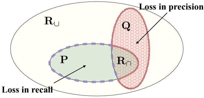
(a) When ${{P}}$ and ${{Q}}$ are uniform we can define natural precision and recall concepts using ${{R}}_{\cup}$ and ${{R}}_{\cap}$, which are uniform on the union and intersection of the supports of ${{P}}$ and ${{Q}}$ respectively.

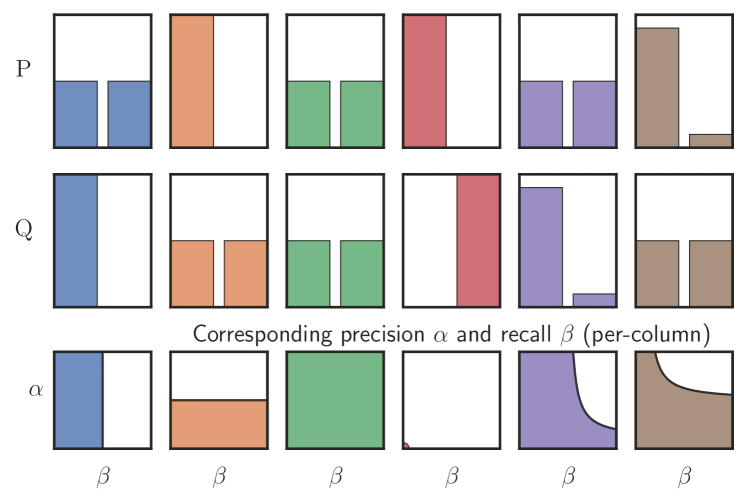
(b) Examples with categorical ${{P}}$ and ${{Q}}$, reproduced from Sajjadi et al., (2018).

Figure 1: For uniform measures we can define natural concepts using set operation (a). Similarly, when they are simple categorical distributions, we would like to generate curves like those in (b).

The central problem considered in the paper is the development of a framework that formalizes the concepts of precision and recall for arbitrary measures, and enables the development of principled evaluation tools. Namely, we want to understand how does a learned model, henceforth denoted by ${{Q}}$, compare to the target distribution ${{P}}$. Informally, to compute the precision we need to estimate how much probability ${{Q}}$ assigns to regions of the space where ${{P}}$ has high probability. Alternatively, to compute the recall we need to estimate how much probability ${{P}}$ assigns to regions of the space that are likely under ${{Q}}$.

Let us start by developing an intuitive understanding of the problem with simple examples where the relationship between ${{P}}$ and ${{Q}}$ is easily understandable. Figure 1 illustrates the case where ${{P}}$ and ${{Q}}$ are uniform distributions with supports ${\textrm{supp}}({{P}})$ and ${\textrm{supp}}({{Q}})$. To help with the exposition of our approach in the next section, we also introduce the distributions ${{R}}_{\cup}$ and ${{R}}_{\cap}$ which are uniform on the union and intersection of the supports of ${{P}}$ and ${{Q}}$ respectively. Then, the loss in precision can then be understood to be proportional to the measure of ${\textrm{supp}}({{Q}})\setminus{\textrm{supp}}({{R}}_{\cap})$ which corresponds to the "part of ${{Q}}$ not covered by ${{P}}$". Analogously, the loss in recall of ${{Q}}$ w.r.t. ${{P}}$ is proportional to the size of ${\textrm{supp}}({{P}})\setminus{\textrm{supp}}({{R}}_{\cap})$ which represents the "part of ${{P}}$ not covered by ${{Q}}$. Note that we can also write these sets as ${\textrm{supp}}({{R}}_{\cup})\setminus{\textrm{supp}}({{P}})$ and ${\textrm{supp}}({{R}}_{\cup})\setminus{\textrm{supp}}({{Q}})$ respectively. The precision and recall are then naturally maximized when ${{P}}={{Q}}$. When the distributions are discrete we would like to generate plots similar to those in Figure 1(b). The first column corresponds to ${{Q}}$ which fails to model one of the modes of ${{P}}$, and the second column to a ${{Q}}$ which has an “extra” mode. We would like our framework to mark these two failure modes as losses in recall and precision, respectively. The third column corresponds to ${{P}}={{Q}}$, followed by a situation where ${{P}}$ and ${{Q}}$ have disjoint support. Finally, for the last two columns, a possible precision-recall trade-off is illustrated. While this intuition is satisfying for uniform and categorical distributions, it is unclear how to extend it to continuous distributions that might be supported on the complete space.

2 DIVERGENCE FRONTIERS

To formally transport these ideas to the general case, we will introduce an auxiliary distribution ${{R}}$ that is constrained to be supported only on those regions where both ${{P}}$ and ${{Q}}$ assign high probability. Informally, this should act as a generalization to the general case of ${{R}}_{\cap}$, which was the measure on the intersection of the supports of ${{P}}$ and ${{Q}}$. Then, the discrepancy between ${{P}}$ and ${{R}}$ measures the space that is likely under ${{P}}$ but not under ${{R}}$, which can be seen as loss in recall. Similarly, the discrepancy between ${{Q}}$ and ${{R}}$ quantifies the size of the space where ${{Q}}$ assigns probability mass, but ${{P}}$ does not, which we can be interpreted as a loss in recall.

Hence, we need both a mechanism to measure distances between distributions and means to constrain ${{R}}$ to assign mass only where both ${{P}}$ and ${{Q}}$ do. For example, if ${{P}}$ and ${{Q}}$ are both mixtures of several components ${{R}}$ should assign mass only to the components shared by both ${{P}}$ and ${{Q}}$.

A dual view  Alternatively, building on the observation from the previous section that both ${{R}}_{\cup}$ and ${{R}}_{\cap}$ can be used to define precision and recall, instead of modeling the intersection of ${{P}}$ and ${{Q}}$, we can use an auxiliary distribution ${{R}}$ to approximate the union of the high-probability regions of ${{P}}$ and ${{Q}}$. Then, using a similar analogy as before, the distance between ${{P}}$ and ${{R}}$ should measure the loss in precision, while the distance between ${{Q}}$ and ${{R}}$ the loss in recall. In this case, ${{R}}$ should give non-zero probability to any part of the space where either ${{P}}$ or ${{Q}}$ assign mass. When ${{P}}$ and ${{Q}}$ are both mixtures of several components, ${{R}}$ has to be supported on the union of all mixture components.

As a result, the choice of the statistical divergence between ${{P}}$, ${{Q}}$ and ${{R}}$ becomes paramount.

2.1 Choice of Divergence

To be able to constrain ${{R}}$ to assign probability mass only in those regions where ${{P}}$ and ${{Q}}$ do, we need a measure of discrepancy between distributions that penalizes differently under- and over-coverage. Even though the theory and concepts introduced in this paper extend to any such divergence, we will focus our attention to the family of Rényi divergences. They not only do exhibit such behavior, but their properties are also well-studied in the literature, which we can leverage to develop a deeper understanding of our approach, and in the design of efficient computational tools.

Definition 1 (Rényi Divergence (Rényi,, 1961)).

Let ${{P}}$ and ${{Q}}$ be two measures such that ${{Q}}$ is absolutely continuous with respect to ${{P}}$, i.e., any measure set with zero measure under ${{P}}$ has also zero measure under ${{Q}}$. Then, the Rényi divergence of order $\alpha\in(0,1)\cup(1,\infty)$ is defined as

$$D_{\alpha}({{P}}\,\|\,{{Q}})=\frac{1}{\alpha-1}\log\int\left(\frac{d{{P}}}{d{{Q}}}\right)^{\alpha-1}d{{P}},$$ (1)

where $d{{P}}/d{{Q}}$ is the Radon-Nikodym derivative.

The fact that they are sensitive to how the supports of ${{P}}$ and ${{Q}}$ relate to one another is already hinted by the constraint in the definition, which requires that ${\textrm{supp}}({{P}})\subseteq{\textrm{supp}}({{Q}})$. Furthermore, by increasing the parameter $\alpha$ the divergence becomes “less forgiving” — for example if ${{P}}$ and ${{Q}}$ are Gaussians with deviations $\sigma_{{P}}$ and $\sigma_{{Q}}$, we have that $D_{\alpha}({{P}}\,\|\,{{Q}})$ increases faster as $\alpha\to\infty$ when $\sigma_{{Q}}$ drops below $\sigma_{{P}}$, while $D_{\alpha}({{Q}}\,\|\,{{P}})$ grows with increasing $\sigma_{{Q}}$ and $\alpha\to\infty$, which we illustrate in Figure 2. This is exactly the property that we need to be able to define meaningful concepts of precision and recall. For a more detailed analysis of this behavior we point the reader to Minka et al., (2005).

Rényi divergences have been extensively studied in the literature (Van Erven and Harremos,, 2014) and many of their properties are well-understood — for example, they are non-negative and zero only if the distributions are equal a.s., and increasing in $\alpha$. Some of their orders are closely related to the Hellinger and $\chi^{2}$ divergences, and it can be further shown that $D_{\textrm{KL}}({{P}}\,\|\,{{Q}})=\int\log(\frac{d{{P}}}{d{{Q}}})d{{P}}=\lim_{\alpha\to 1}D_{\alpha}({{P}}\,\|\,{{Q}})$.

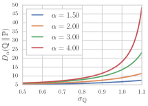
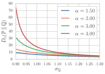
Figure 2: Rényi divergences strongly penalize when the first argument assigns mass away from the high probability regions of the second. We analytically evaluate $D_{\alpha}$, where $\mathbb{P}$ is a Normal (Gil et al.,, 2013).

2.2 Divergence Frontiers

Having defined a suitable discrepancy measure, we are ready to define the central concepts in this paper, which will play the role of precision-recall curves for arbitrary measures. To do so, we will not put hard constraints on ${{R}}$, but only softly enforce them. Namely, consider the case when we want ${{R}}$ to model the intersection of the high likelihood regions of ${{P}}$ and ${{Q}}$. Then, if it fails to do so, either $D_{\alpha}({{R}}\,\|\,{{P}})$ or $D_{\alpha}({{R}}\,\|\,{{Q}})$ will be significantly large. Similarly, unless ${{R}}$ fails to assign large probabilities to the high likelihood regions of both ${{P}}$ and ${{Q}}$, at least one of $D_{\alpha}({{P}}\,\|\,{{R}})$ and $D_{\alpha}({{Q}}\,\|\,{{R}})$ will be large. Thus, we will only consider those ${{R}}$ that simultaneously minimize both divergences, which motivates the following definition.

Definition 2 (Divergence frontiers).

For any two measures ${{P}}$ and ${{Q}}$, any class of measures $\mathcal{M}$ and any $\alpha\geq 0$, we define the exclusive realizable region as the set

$${{\mathcal{R}}}^{\cap}_{\alpha}({{P}},{{Q}})=\{(D_{\alpha}({{R}}\,\|\,{{Q}}),D_{\alpha}({{R}}\,\|\,{{P}}))\mid{{R}}\in\mathcal{M}\},$$ (2)

and the inclusive realizable region $\mathcal{R}^{\cup}_{\alpha}({{P}},{{Q}})$ by swapping the arguments of $D_{\alpha}$ in (2). The exclusive and inclusive divergence frontiers are then defined as the maximal points of the corresponding realizable regions

$${\mathcal{F}}^{\cap}_{\alpha}({{P}},{{Q}}\mid\mathcal{M})= \{(\pi,\rho)\in{\mathcal{R}}^{\cap}_{\alpha}({{P}},{{Q}}\mid\mathcal{M})$$

$$\mid\nexists(\pi^{\prime},\rho^{\prime})\in{\mathcal{R}}^{\cap}({{P}},{{Q}})$$

$$\textrm{ s.t.\ }\pi^{\prime}<\pi\textrm{ and }\rho^{\prime}<\rho\},$$

and $\mathcal{F}^{\cup}_{\alpha}$ is defined by replacing $\mathcal{R}^{\cap}$ with $\mathcal{R}^{\cup}$.

In other words, we want to compute the Pareto frontiers of the multi-objective optimization problem with the divergence minimization objectives $f_{1}({{R}})=D_{\alpha}({{R}}\,\|\,{{Q}}),f_{2}({{R}})=D_{\alpha}({{R}}\,\|\,{{P}})$ and $f_{3}({{R}})=D_{\alpha}({{Q}}\,\|\,{{R}}),f_{4}({{R}})=D_{\alpha}({{P}}\,\|\,{{R}})$ respectively. In machine learning such divergence minimization problems appear in approximate inference. Interestingly, $f_{1}$ and $f_{2}$ are the central object one minimizes in variational inference (VI) (Wainwright et al.,, 2008, §5)(Li and Turner,, 2016), while $f_{3}$ and $f_{4}$ are exactly the objectives in expectation propagation (EP) (Minka,, 2001; Minka et al.,, 2005). Hence, the problem of computing the frontiers can be seen as that of performing VI or EP with two target distributions instead of one.

3 CHARACTERIZATION OF THE FRONTIERS

Having defined the frontiers, we now characterize them, so that we can discuss their computation in the next section. Remember that to compute the frontiers we have to characterize the subset of ${\mathbb{R}}^{2}$ consisting of all pairs $(D_{\alpha}({{R}}\,\|\,{{P}}),D_{\alpha}({{R}}\,\|\,{{Q}}))$ and $(D_{\alpha}({{P}}\,\|\,{{R}}),D_{\alpha}({{Q}}\,\|\,{{R}}))$ which are not strictly dominated. To solve these two multi-objective optimization problem we scalarize them by optimizing the problems

$${{R}}^{\cup}_{\alpha,\lambda} =\operatorname*{arg\,min}_{{{R}}}\lambda\hat{D}_{\alpha}({{Q}}\,\|\,{{R}})+(1-\lambda)\hat{D}_{\alpha}({{P}}\,\|\,{{R}})$$ (3)

$${{R}}^{\cap}_{\alpha,\lambda} =\operatorname*{arg\,min}_{{{R}}}\lambda\hat{D}_{\alpha}({{R}}\,\|\,{{Q}})+(1-\lambda)\hat{D}_{\alpha}({{R}}\,\|\,{{P}}).$$ (4)

where $\hat{D}_{\alpha}=\frac{1}{\alpha-1}e^{\frac{D_{\alpha}}{\alpha-1}}$ is a monotone function of the Rényi divergence. We then vary $\lambda\in[0,1]$ and plug ${{R}}_{\alpha,\lambda}$ back in $D_{\alpha}$ to obtain the frontier.

Fortunately, this problem can be analytically solved. The discrete case has been solved by Nielsen and Nock, (2009, III), and we modify their argument to the continuous case.

Proposition 1.

Let ${{P}}$ and ${{Q}}$ be two measures with densities $p$ and $q$ respectively. Then, the distribution minimizing $\eqref{eqn:left-barycenter}$ has density

$$\quad r_{\alpha,\lambda}(x)\propto(\lambda q(x)^{1-\alpha}+(1-\lambda)p(x)^{1-\alpha})^{1/(1-\alpha)}.$$

Similarly, the optimizer of $\eqref{eqn:right-barycenter}$ is minimized at the distribution with density

$$\quad r_{\alpha,\lambda}(x)\propto(\lambda q(x)^{\alpha}+(1-\lambda)p(x)^{\alpha})^{1/\alpha}.$$

Proof sketch.

In the inclusive case, (3) is equal to

$$\hat{D}_{\alpha}({{R}}_{\alpha,\lambda}^{\cap}\,\|\,{{R}})\int(\lambda q(x)^{\alpha}+(1-\lambda p(x)^{\alpha}))^{1/\alpha}dx,$$

which is minimized when ${{R}}={{R}}_{\alpha,\lambda}^{\cap}$ as the first term is a divergence, and the second term is constant with respect to ${{R}}$. The exclusive case is analogous. ∎

Even thought not the case for general problems, linear scalarization does yield the correct frontier due to the properties of the Rényi divergences.

Proposition 2.

For any measures ${{P}}$ and ${{Q}}$ with densities $p$ and $q$ respectively, we can compute the exclusive frontier as

$${{\mathcal{F}^{\cap}}}_{\alpha}(P,Q)=\{(D_{\alpha}(R^{\cap}_{\alpha,\lambda}\,\|\,{{P}}),D_{\alpha}(R^{\cap}_{\alpha,\lambda}\,\|\,{{Q}}))\mid\lambda\in[0,1]\},$$

and the inclusive frontier is given as

$${{\mathcal{F}^{\cup}}}_{\alpha}(P,Q)=\{(D_{\alpha}({{P}}\,\|\,R^{\cup}_{\alpha,\lambda}),D_{\alpha}({{Q}}\,\|\,R^{\cup}_{\alpha,\lambda}))\mid\lambda\in[0,1]\}.$$

Proof sketch.

Even though $D_{\alpha}$ is not jointly convex, we can write it as a monotone function of an $f$-divergence, which is jointly convex function and lets us utilize results from multi-objective convex optimization. ∎

4 COMPUTING THE FRONTIERS

We will now discuss how to compute the divergences when we have access to the distributions. We discuss strategies for how to do this in practice in §6.

4.1 Discrete Measures

When the distributions take on one of $n$ values, the solution is obtain by simply replacing the integrals with sum in 2. Hence, if we discretize $\lambda$ over a grid of size $k$, we will have a total complexity of $O(nk)$. Furthermore, this case has a very nice geometrical interpretation associated with it. Namely, in this case we can represent the distributions as vectors in the simplex $\Delta=\{{\bm{\mu}}\in[0,1]^{n}\mid\bm{1}^{\top}{\bm{\mu}}=1\}$, and use ${\mathbf{p}}\in\Delta$ for ${{P}}$ and ${\mathbf{q}}\in\Delta$ for ${{Q}}$. Then, conceptually, to compute the frontier we walk along the path ${{R}}_{\alpha,\gamma}$ from ${\mathbf{p}}$ to ${\mathbf{q}}$, and at each point we compute the distances to ${\mathbf{p}}$ and ${\mathbf{q}}$ as measured by $D_{\alpha}$. We illustrate this in Figure 3.

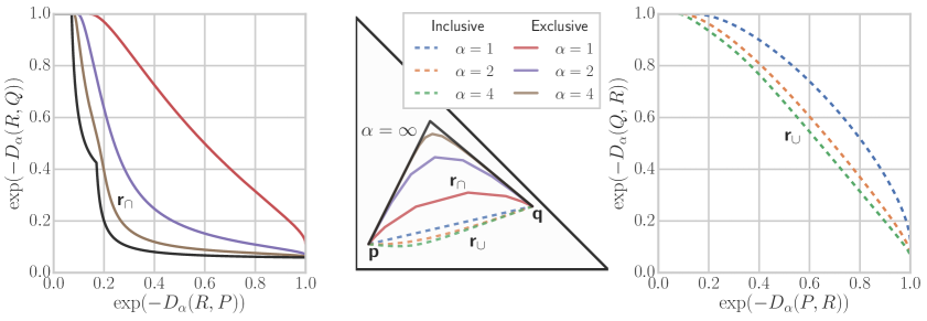
Figure 3: Illustration of the algorithm computing the discrete frontiers. In the middle panel we show two measures ${\mathbf{p}}$ and ${\mathbf{q}}$ on the probability simplex, together with the barycentric paths $\gamma(\lambda)$ between them for various $\alpha$. These paths in turn generate the inclusive (left) and exclusive (right) frontiers. The limiting $\alpha=\infty$ exclusive case coincides with the precision-recall curve from Sajjadi et al., (2018) (c.f. §5).

4.2 Integration

The frontiers can be also written as integrals of functions of the density ratio $p(x)/q(x)$ over the measures ${{P}}$ and ${{Q}}$, which has practical implications, discussed in Section 6. Specifically, we have the following result.

Proposition 3.

Define for any $\beta,\lambda$ the functions $u_{\gamma}^{\beta}(t)=(\gamma+(1-\gamma)t^{\beta})^{(1-\beta)/\beta}$ and $v_{\gamma}^{\beta}(t)=(\gamma+(1-\gamma)t^{\beta})^{1/\beta}$. The exclusive frontier ${{\mathcal{F}^{\cap}}}_{\alpha}({{P}},{{Q}})$ equals

$$\{( \frac{1}{\alpha-1}\log\mathbb{E}_{P}[u_{\lambda}^{1-\alpha}(\frac{p(x)}{q(x)})]-\frac{\alpha}{\alpha-1}\log\mathbb{E}_{P}[v_{\lambda}^{1-\alpha}(\frac{p(x)}{q(x)})],$$

$$\frac{1}{\alpha-1}\log\mathbb{E}_{Q}[u_{1-\lambda}^{1-\alpha}(\frac{q(x)}{p(x)})]-\frac{\alpha}{\alpha-1}\log\mathbb{E}_{Q}[v_{1-\lambda}^{1-\alpha}(\frac{q(x)}{p(x)})]\}.$$

The inclusive frontier is obtained by changing $u_{\gamma}^{1-\alpha}$ to $u_{\gamma}^{\alpha}$, $v_{\gamma}^{1-\alpha}$ to $v_{\gamma}^{\alpha}$, and $-\alpha/(\alpha-1)$ to $1$.

Note that the naïve plug-in estimator would result in a biased estimate due to the fact that the expectation is inside the logarithm. Similar problems also arise when doing variational inference with Rényi divergences, as discussed in Li and Turner, (2016), who analyze the bias and the behaviour as a function of the sample size.

4.3 Exponential families

The computation of the integrals above can be very challenging even if we know the densities due to the possible high dimensionality of the ambient space. Fortunately, there exists a class of distributions that includes many commonly used distributions called the exponential family, whose frontiers for $\alpha=1$ (i.e., the KL divergence) can be efficiently computed. This not only includes many popular continuous distributions such as the normal and the exponential, but also many discrete distributions, e.g., tractable Markov Random Fields (Wainwright et al.,, 2008) which are common models in vision and natural language processing.

Definition 3 (Exponential families (Wainwright et al.,, 2008, §3.2)).

The exponential family over a domain $\mathcal{X}$ for a sufficient statistic $\nu\colon\mathcal{X}\to\mathbb{R}^{m}$ is the set of all distributions of the form

$$P(x\mid{\bm{\theta}})=\exp({\bm{\theta}}^{\top}\nu(x)-A({\bm{\theta}})),$$ (5)

where ${\bm{\theta}}$ is the parameter vector, and $A({\bm{\theta}})$ is the log-partition function normalizing the distribution.

Importantly, the KL divergence between two distributions in the exponential family with parameters ${\bm{\theta}}$ and ${\bm{\theta}}^{\prime}$ can be computed in closed form as the following Bregman divergence (Wainwright et al.,, 2008, §5.2.2)

$$D_{\textrm{KL}}(P(\cdot\mid{\bm{\theta}})\,\|\,P(\cdot\mid{\bm{\theta}}^{\prime}))=A({\bm{\theta}}^{\prime})-A({\bm{\theta}})-\nabla A({\bm{\theta}})^{\top}({\bm{\theta}}^{\prime}-{\bm{\theta}}),$$

which we shall denote as $D_{\textrm{KL}}({\bm{\theta}}\,\|\,{\bm{\theta}}^{\prime})$. We can now show how to compute the frontier.

Proposition 4.

Let $\mathcal{M}$ be an exponential family with log-partition function $A$. Let ${{P}}$ and ${{Q}}$ be elements in $\mathcal{M}$ with parameters ${\bm{\theta}}_{{P}}$ and ${\bm{\theta}}_{{Q}}$. Then,

• Inclusive: If we define $\gamma(\lambda)=(\nabla A)^{-1}(\lambda\nabla A({\bm{\theta}}_{{P}})+(1-\lambda)\nabla A({\bm{\theta}}_{{Q}}))$, then ${{\mathcal{F}^{\cup}}}_{1}({{P}},{{Q}}\mid\mathcal{M})$ is equal to

  $$\{(D_{\textrm{KL}}({\bm{\theta}}_{{P}}\,\|\,\gamma(\lambda)),D_{\textrm{KL}}({\bm{\theta}}_{{Q}}\,\|\,\gamma(\lambda)))\mid\lambda\in[0,1]\}.$$

• Exclusive: If we define $\gamma(\lambda)=\lambda{\bm{\theta}}_{{P}}+(1-\lambda){\bm{\theta}}_{{Q}}$, then ${{\mathcal{F}^{\cap}}}_{1}({{P}},{{Q}}\mid\mathcal{M})$ is equal to

  $$\{(D_{\textrm{KL}}(\gamma(\lambda)\,\|\,{\bm{\theta}}_{{P}}),D_{\textrm{KL}}(\gamma(\lambda)\,\|\,{\bm{\theta}}_{{Q}})) \mid\lambda\in[0,1]\}.$$

  Furthermore, the frontier will not change if we enlarge $\mathcal{M}$.

Proof sketch.

As the KL divergence is convex in the parameter ${\bm{\theta}}^{\prime}$ of the second distribution, for the inclusive case we can only consider the scalarized objective, which has the claimed closed form solution. In the exclusive case, we use the Bregman divergence generated by the convex conjugate $A^{*}$, which effectively swaps the arguments, and the argument is the same. ∎

5 CONNECTIONS TO EXISTING WORK

Figure 4: The points used in the definition of PRD (Sajjadi et al.,, 2018). For fixed ${\mathbf{p}},{\mathbf{q}}$ and ${\mathbf{r}}$, the points ${\mathbf{p}}^{\prime}$ and ${\mathbf{q}}^{\prime}$ must be lie on the rays ${\mathbf{r}}\to{\mathbf{q}}$ and ${\mathbf{r}}\to{\mathbf{p}}$ respectively. The optimal precision and recall are obtained by taking ${\mathbf{q}}^{\prime}$ and ${\mathbf{r}}^{\prime}$ to lie on the boundary. To compute the frontier we have to consider only those ${\mathbf{r}}$ on the geodesic between ${\mathbf{q}}$ and ${\mathbf{p}}$, shown as the red curve.

Having introduced and showed how to compute the divergence frontiers, we will now present several existing techniques, and show how they relate to our approach.

Rather than computing trade-off curves, Kynkäänniemi et al., (2019) focus only on ${{P}}({\textrm{supp}}({{Q}}))$ and ${{Q}}({\textrm{supp}}({{P}}))$, and estimate the supports using a union of $k$-nearest neighbourhood balls. This is indeed a special case of our framework, as $\lim_{\alpha\to 0}D_{\alpha}({{P}}\,\|\,{{Q}})=-\log{{Q}}({\textrm{supp}}({{P}}))$ (Van Erven and Harremos,, 2014, Thm. 4). One drawback of this approach is that all regions where ${{P}}$ and ${{Q}}$ place any mass are considered equal (see Fig. 5).

We will now show that the approach of (Sajjadi et al.,, 2018) corresponds to the case where $\alpha\rightarrow\infty$. In particular, Sajjadi et al., (2018) write both ${{P}}$ and ${{Q}}$ as mixtures with a shared component that should capture the space that they both assign high likelihood to, and which can be used to formalize the notions of precision and recall for distributions.

Definition 4 ((Sajjadi et al.,, 2018, Def. 1)).

For $\pi,\rho\in(0,1]$, the probability distribution ${{Q}}$ has precision $\pi$ at recall $\rho$ w.r.t. ${{P}}$ if there exist distributions ${{R}},{{P}}^{\prime},{{Q}}^{\prime}$ such that

$${{P}}=\rho{{R}}+(1-\rho){{P}}^{\prime},\textrm{ and }{{Q}}=\pi{{R}}+(1-\pi){{Q}}^{\prime}.$$ (6)

The union of $\{(0,0)\}$ and all realizable pairs $(\pi,\rho)$ will be denoted by $\textsc{PRD}({{P}},{{Q}})$.

Even though the divergence frontiers introduced in this work might seem unrelated to this formalization, there is a clear connection between them, which we now establish. As Sajjadi et al., (2018) target discrete measures, let us treat the distributions as vectors in the probability simplex $\Delta$ and use ${\mathbf{p}}\in\Delta$ for ${{P}}$ and ${\mathbf{q}}\in\Delta$ for ${{Q}}$. We need to consider three additional distributions to compute ${\textsc{PRD}}({\mathbf{p}},{\mathbf{q}})$: ${\mathbf{r}}$, and the per-distribution mixtures ${\mathbf{p}}^{\prime}$ and ${\mathbf{q}}^{\prime}$. These distributions are arranged as shown in Figure 4. Because ${\mathbf{r}},{\mathbf{p}}$ and ${\mathbf{p}}^{\prime}$ are co-linear and ${\mathbf{p}}=\rho{\mathbf{r}}+(1-\rho){\mathbf{p}}^{\prime}$, we have that the recall obtained for this configuration is $\|{\mathbf{p}}-{\mathbf{p}}^{\prime}\|/\|{\mathbf{r}}-{\mathbf{p}}^{\prime}\|$. Similarly, the precision $\pi$ can be easily seen to be equal to $\|{\mathbf{q}}-{\mathbf{q}}^{\prime}\|/\|{\mathbf{r}}-{\mathbf{q}}^{\prime}\|$. Most importantly, we can only increase both $\rho$ and $\pi$ if we move ${\mathbf{p}}^{\prime}$ and ${\mathbf{q}}^{\prime}$ along the rays ${\mathbf{r}}\to{\mathbf{p}}$ and ${\mathbf{r}}\to{\mathbf{q}}$, respectively. Specifically, the maximal recall $\rho^{*}$ and precision $\pi^{*}$ for this fixed ${\mathbf{r}}$ are obtained when ${\mathbf{p}}^{\prime}$ and ${\mathbf{q}}^{\prime}$ are as far as possible from ${\mathbf{r}}$, i.e., when they lie on the boundary $\partial\Delta$. To formalize this, let us denote for any $\mathbf{a},\mathbf{b}$ in $\Delta$ by $\partial_{\Delta}(\mathbf{a},\mathbf{b})$ the point along the ray $\mathbf{a}\to\mathbf{b}$ that intersects the boundary of $\Delta$. Then, the maximal $\pi$ and $\rho$ are achieved for ${\mathbf{p}}^{\prime}=\partial_{\Delta}({\mathbf{r}},{\mathbf{p}})$ and ${\mathbf{q}}^{\prime}=\partial_{\Delta}({\mathbf{r}},{\mathbf{q}})$. Perhaps surprisingly, these best achievable precision and recall have been already studied in geometry and have very remarkable properties, as they give rise to a weak metric.

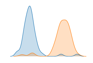
Figure 5: A case where the metric defined by Kynkäänniemi et al., (2019) would result in essentially perfect precision and perfect recall. Arguably, these distributions are very different.

Definition 5 ((Papadopoulos and Yamada,, 2013, Def. 2.1)).

The Funk weak metric $F_{\Delta}\colon\Delta^{2}\to[0,\infty)$ on $\Delta$ is defined by

$$F_{\Delta}({\mathbf{p}},{\mathbf{p}}) =0,\textrm{and }$$

$$F_{\Delta}({\mathbf{p}},{\mathbf{q}}) =\log(\|{\mathbf{p}}-\partial_{\Delta}({\mathbf{p}},{\mathbf{q}})\|/\|{\mathbf{q}}-\partial_{\Delta}({\mathbf{p}},{\mathbf{q}})\|).$$

Furthermore, we have that the Funk metric coincides with a limiting Rényi divergence.

Proposition 5 ((Papadopoulos and Troyanov,, 2014, Ex. 4.1),(Van Erven and Harremos,, 2014, Thm. 6)).

For any ${\mathbf{p}},{\mathbf{q}}$ in the probability simplex $\Delta$, we have that

$$F_{\Delta}({\mathbf{p}},{\mathbf{q}})=\lim_{\alpha\to\infty}D_{\alpha}({\mathbf{p}}\,\|\,{\mathbf{q}})=\log\max_{i=1}^{n}p_{i}/q_{i}$$

This immediately implies the following connection between the set of maximal points in ${\textsc{PRD}}({{P}},{{Q}})$, which we shall denote by $\overline{{\textsc{PRD}}}({{P}},{{Q}})$ and $\mathcal{F}^{\cap}_{\infty}({\mathbf{p}},{\mathbf{q}})$. In other words, the maximal points in PRD coincide with one of the exclusive frontiers we have introduced.

Proposition 6.

For any distributions ${{P}},{{Q}}$ on $\{1,2,\ldots,n\}$ it holds that

$$\overline{{\textsc{PRD}}}({{P}},{{Q}})=\{(e^{-\pi},e^{-\rho})\mid(\rho,\pi)\in\mathcal{F}_{\infty}^{\cap}({{P}},{{Q}})\}.$$

Furthermore, the fact that $D_{\infty}$ is a weak metric implies that, in contrast to the $\alpha<\infty$ case, the triangle inequality holds (Papadopoulos and Yamada,, 2013, Thm. 7.1). As a result, we can make an even stronger claim — the path taken by the distributions ${\mathbf{r}}$ that generate the frontier is the shortest in the corresponding geometry.

Proposition 7.

Let us define the curve $\gamma(\lambda)\colon[\min_{i}\frac{q_{i}}{p_{i}},\max_{i}\frac{q_{i}}{p_{i}}]\to\Delta$ as

$$[\gamma(\lambda)]_{i}\propto\min\{p_{i},q_{i}/\lambda\}.$$

$$\textrm{Then, }\,\mathcal{F}_{\infty}^{\cap}({\mathbf{p}},{\mathbf{q}})=\{ (D_{\infty}(\gamma(\lambda)\,\|\,{\mathbf{p}}),D_{\infty}(\gamma(\lambda)\,\|\,{\mathbf{q}}))$$

$$\mid\lambda\in[\min_{i}\frac{q_{i}}{p_{i}},\max_{i}\frac{q_{i}}{p_{i}}]\},$$

and, moreover, $\gamma(\lambda)$ is geodesic, i.e., it evaluates at the endpoints to ${\mathbf{p}}$ and ${\mathbf{q}}$, and for any $\lambda$

$$F_{\Delta}({\mathbf{p}},{\mathbf{q}})=F_{\Delta}({\mathbf{p}},\gamma(\lambda))+F_{\Delta}(\gamma(\lambda),{\mathbf{q}}).$$

Simon et al., (2019) extend this approach to continuous models by showing that that PRD  can be computed by thresholding the density ratio $p(x)/q(x)$, which they approximate using binary classification. In Section 4.2 we have extended this result to arbitrary divergences.

Finally, we note that the idea of precision and recall for generative models also appeared in Lucic et al., (2018) and was used for quantitatively evaluating generative adversarial networks and variational autoencoders, by considering a synthetic data set for which the data manifold is known and the distance from each sample to the manifold could be computed.

6 PRACTICAL APPROACHES AND CONSIDERATIONS

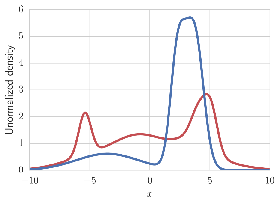
(a) The distributions we quantize.

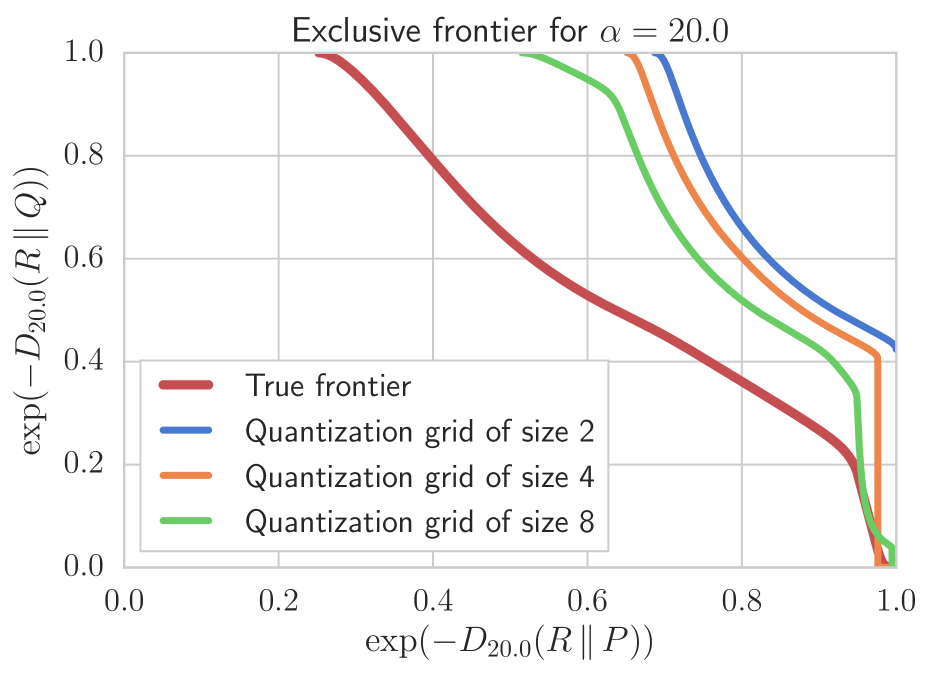
(b) Biases from coarse quantization.

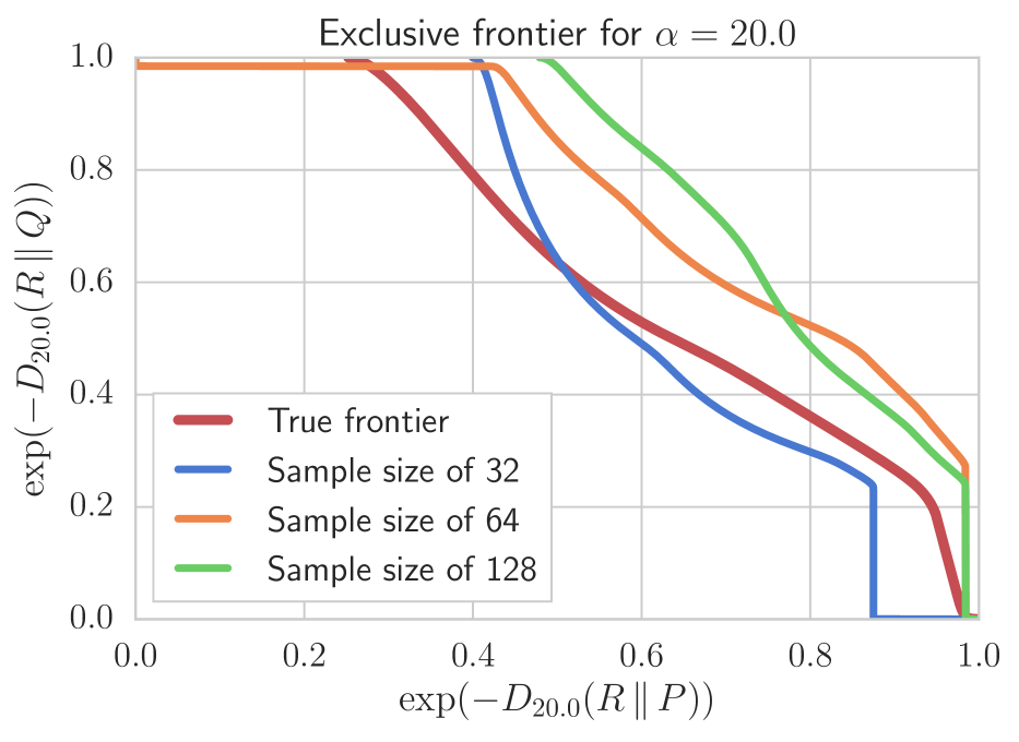
(c) Noise from small samples.

Figure 6: The systemic biases when we compute the frontiers after quantizing the distributions in (a). In (b) we see that using too few buckets can result in overly optimistic results. In (c) we show that if an insufficient number of samples is used, the curves might fluctuate and look pessimistic.

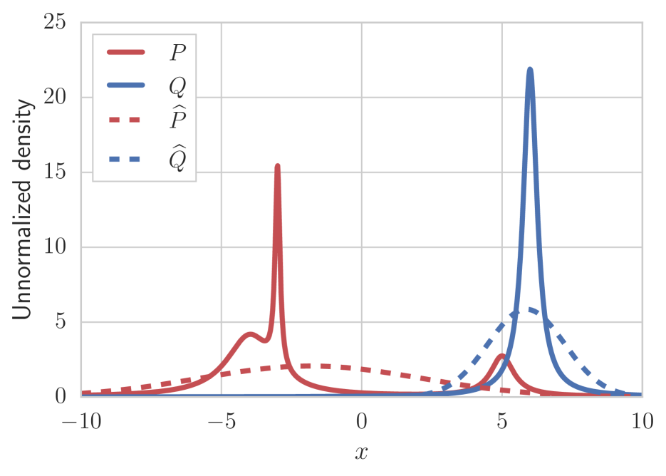
(a) The distributions we compare and their Gaussian approximations.

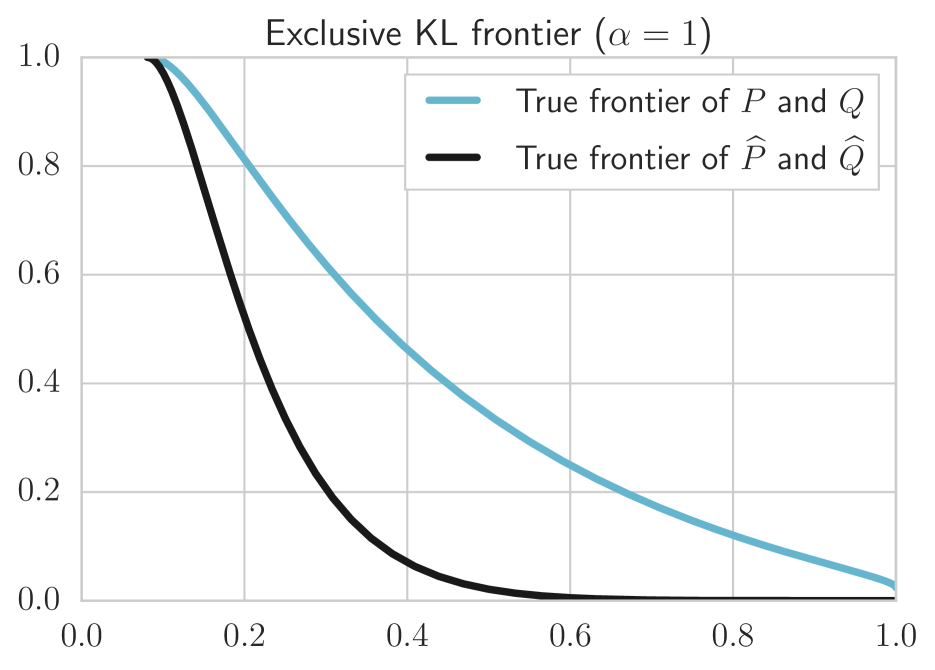
(b) Estimating the exclusive frontier using Gaussian approximations.

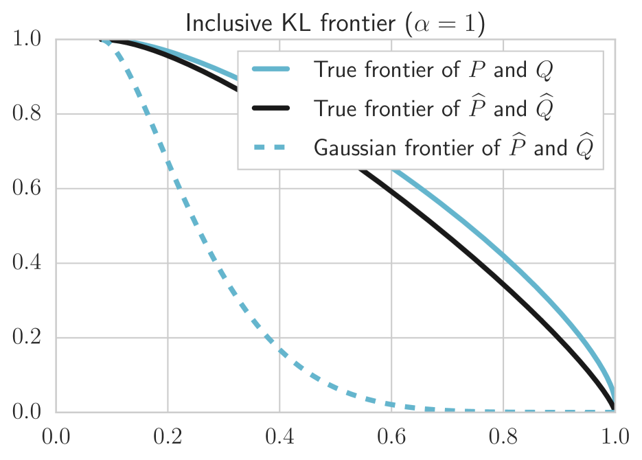
(c) Estimating the inclusive frontier using Gaussian approximations.

Figure 7: Estimating the frontier by approximating the distributions with Gaussians. In (b) we see that the exclusive frontier can look more pessimistic than the truth. Panel (c) shows that using distributions $R$ that are further restricted to also be Gaussian can make matters worse when computing the inclusive frontier. Note that in (b) there is no such curve as it agrees with the true frontier (black line) due to the last claim in 4.

In practice, when we are tasked with the problem of evaluating a model, we typically only have access to samples from ${{P}}$ and ${{Q}}$, and optionally also the density of ${{Q}}$. There are many approaches one can undertake when applying the methods developed in this paper to generate precision-recall curves. In what follows we discuss several of these, and highlight their benefits, but also some of their drawbacks. We would like to point out that in the case of image synthesis, the comparison is typically not done in the original high-dimensional image space, but (as done in Sajjadi et al., (2018); Kynkäänniemi et al., (2019); Heusel et al., (2017)) in feature spaces where distances are expected to correlate more strongly with perceptual difference.

Quantization  One strategy would be to discretize the data, as done in (Sajjadi et al.,, 2018), and then apply the methods from Section 4.1. Even though estimating the divergences between categorical distributions is simple and in the limit converges to the continuous $\alpha$ divergence (Van Erven and Harremos,, 2014, Thm. 2), there may be several issues with this approach. For example, this approach will inherently introduce a positively bias for any discretization and any $\alpha$. Namely, the generated curves will always look better than the truth, which we formalize below.

Proposition 8.

Let ${{P}}$ and ${{Q}}$ be distributions that have been quantized into the discrete distributions $\hat{{{P}}}$ and $\hat{{{Q}}}$ respectively. Then, it holds that

$$\mathcal{R}^{\cap}_{\alpha}(\hat{{{P}}},\hat{{{Q}}})\subseteq\mathcal{R}^{\cap}_{\alpha}({{P}},{{Q}})\textrm{ and }\mathcal{R}^{\cup}_{\alpha}(\hat{{{P}}},\hat{{{Q}}})\subseteq\mathcal{R}^{\cup}_{\alpha}({{P}},{{Q}}).$$

Moreover, if we do not have enough samples to estimate the fraction of points that fall in each partition, we might see very strong fluctuations of the curves. This is due to the fact that the divergences penalize heavily situations when one distributions puts zero mass on the support of the other and the distributions might appear more distant than the truth. We illustrate both of these situations on two one dimensional distributions in Figure 6. We can see that discretization indeed has a positive bias, and that small sample sizes can result in overly pessimistic curves. Furthermore, in high-dimensions the result will also depend on the quality of the clustering, which in general is NP-hard and has additional hyperparameters that can be hard to tune.

Exponential families  Alternatively, one can estimate ${{P}}$ and ${{Q}}$ from samples using maximum likelihood over some exponential family $\mathcal{M}$, and then apply the methods from Section 4.3, which result in analytical frontiers. While this might seem simplistic, fitting multivariate Gaussians has been shown to work well for evaluating generative models using the FID score (Heusel et al.,, 2017). Even though projecting ${{P}}$ and ${{Q}}$ onto some exponential family might suggest that it will always make them closer and thus result in a positive bias, this it not necessarily always the case. We show in Figure 7 a setting where the opposite happens. What we can formally show, however, is that the inclusive frontier will have a positive bias when the distribution ${{R}}$ we optimize over is restricted to $\mathcal{M}$.

Proposition 9.

Let ${{P}}$ and ${{Q}}$ be distributions with maximum likelihood estimates $\hat{P}$ and $\hat{Q}$ belonging to some exponential family $\mathcal{M}$ Then, it holds that

$$\mathcal{R}_{1}^{\cup}({{P}},{{Q}}\mid\mathcal{M})\subseteq\mathcal{R}_{1}^{\cup}(\hat{P},\hat{Q}\mid\mathcal{M}).$$

Proof sketch.

To show this result we rely on the fact that maximum likelihood estimation is equivalent to (reverse-)projection under the KL divergence, and the fact the KL divergence satisfies a generalized Pythagorean inequality (Csiszár and Matus,, 2003). ∎

Density ratio estimation  Similarly to (Simon et al.,, 2019), one can first estimate the log ratio $p(x)/q(x)$ by fitting a binary classifier (Sugiyama et al.,, 2012), and then approximate the terms in Section 4.2 using Monte Carlo. One can also tune the loss function to match the integrands, as suggested by Menon and Ong, (2016). However, precisely estimating the density ratio is challenging, and large sample sizes might be needed as the estimator is biased.

Directly estimating $F_{1}^{\cup}$  The inclusive frontier for $\alpha=1$ is valid even when we use empirical distributions for ${{P}}$ and ${{Q}}$ without fitting any models. In this case, it can be easily seen that if we optimize $R_{1,\lambda}^{\cup}$ over some family $\mathcal{M}$, that this is equivalent to maximum likelihood estimation where the samples come from the mixture $\lambda{{P}}+(1-\lambda){{Q}}$. Hence, if we employ flexible density estimators $\mathcal{M}$, one strategy would be to (i) first fit a model on the weighted dataset, and then (ii) evaluate the likelihoods when the data is generated under $P$ and $Q$ on a separate test set.

7 CONCLUSIONS

We developed a framework for comparing distributions via the Pareto frontiers of information divergences, and fully characterized them using efficient computational algorithms for a large family of distributions. We recovered previous approaches as special cases, and thus provided a novel perspective on them and their algorithms. Furthermore, we believe that we have also opened many interesting research questions related to classical approximate inference methods — can we use different divergences or extend the algorithms to even richer model families, and how to identify the correct approach for approximating the frontiers when we only have access to samples.

Appendix A Proofs

Proof of 6.

Even though this result follows clearly from the discussion just above the claim, we provide it for completeness. Namely, let $(\pi,\rho)\in\overline{{\textsc{PRD}}}$ be generated for some ${\mathbf{p}},{\mathbf{q}},{\mathbf{r}}$. Based on the argument below 4 it follows that it must be equal to $(\pi,\rho)=(e^{-F_{\Delta}({\mathbf{r}},{\mathbf{q}})},e^{-F_{\Delta}({\mathbf{r}},{\mathbf{q}})})$. Then, the pair $(\pi,\rho)$ is maximal in PRD iff $(F_{\Delta}({\mathbf{r}},{\mathbf{p}}),F_{\Delta}({\mathbf{r}},{\mathbf{q}}))$ is minimal in $\mathcal{R}^{\cap}_{\infty}({{P}},{{Q}})$, i.e., iff $(F_{\Delta}({\mathbf{r}},{\mathbf{p}}),F_{\Delta}({\mathbf{r}},{\mathbf{q}}))\in\mathcal{F}^{\cap}_{\infty}({{P}},{{Q}})$. ∎

Proof of 7.

If we also include the normalizer of $\gamma(\lambda)$, we have that

$$[\gamma(\lambda)]_{i}=\min\{p_{i},q_{i}/\lambda\}/\beta(\lambda),\textrm{ where }\beta(\lambda)=\sum_{i=1}^{n}\min\{p_{i},q_{i}/\lambda\}.$$

The end-point condition is easy to check, namely

$$[\gamma\min_{j}\{q_{j}/p_{j}\})]_{i} =\min\{p_{i},\frac{q_{i}}{\min_{j}\{q_{j}/p_{j}\}}\}/\beta(\lambda)=p_{i}/\beta(\lambda)=p_{i},\textrm{ and}$$

$$[\gamma(\min_{j}\{q_{j}/p_{j}\})]_{i} =\min\{p_{i},\frac{q_{i}}{\max_{j}\{q_{j}/p_{j}\}}\}/\beta(\lambda)=q_{i}/\beta(\lambda)=q_{i}.$$

Let us now show that $\log\beta(\lambda)=-F_{\Delta}(\gamma(\lambda),{\mathbf{q}})$. The right hand side can be re-written as

$$F_{\Delta}(\gamma(\lambda),{\mathbf{p}})=\log\max_{i}\frac{\min\{p_{i},q_{i}/\lambda\}/\beta(\lambda)}{p_{i}}=-\log\beta(\lambda)+\log\max_{i}\min\{1,\frac{q_{i}}{p_{i}\lambda}\}.$$

Note that the term inside the log is not one only if $q_{i}/p_{i}<\lambda$ for all $i$, which can happen only if $\lambda>\max_{i}\frac{q_{i}}{p_{i}}$, which is outside the domain of $\gamma$. Similarly,

$$F_{\Delta}(\gamma(\lambda),{\mathbf{q}}) =\log\max_{i}\frac{\min\{p_{i},q_{i}/\lambda\}/\beta(\lambda)}{q_{i}}$$

$$=-\log\beta(\lambda)+\log\max_{i}\min\{\frac{p_{i}}{q_{i}},1/\lambda\}$$

$$=-\log\beta(\lambda)\lambda+\log\max_{i}\min\{\frac{\lambda p_{i}}{q_{i}},1\}.$$

The claim follows because $\alpha(\lambda)=\lambda\beta(\gamma)$, and by noting that the maximum inside the logarithm is strictly less than one only if for all $i$ it holds that $\lambda<\frac{q_{i}}{p_{i}}$, which is outside the domain of $\gamma$.

Finally, let us show the geodesity of the curve.

$$F_{\Delta}({\mathbf{p}},{\bm{\mu}}^{*}(\lambda))+F_{\Delta}({\bm{\mu}}^{*}(\lambda),{\mathbf{q}}) =\log\max_{i}\frac{p_{i}}{\min\{p_{i},q_{i}/\lambda\}/\beta(\lambda)}+\log\max_{i}\frac{\min\{p_{i},q_{i}/\lambda\}/\beta(\lambda)}{q_{i}}$$

$$=\max_{i}\log\max\{\log\frac{\lambda p_{i}}{q_{i}},1\}+\max_{i}\log\min\{\frac{p_{i}}{q_{i}},\frac{1}{\lambda}\}$$

• Case (i): $\lambda\geq\max_{i}\frac{q_{i}}{p_{i}}$. Then, $\frac{\lambda p_{i}}{q_{i}}\lambda\geq 1$, so that the first term will be equal to $\log\lambda+\log\max_{i}\frac{p_{i}}{q_{i}}$. Similarly, $\lambda^{-1}\leq\frac{p_{i}}{q_{i}}$, so that the second term is equal to $-\log\lambda$, and the claimed equality is satisfied.

• Case (ii): $\lambda<\max_{i}\frac{q_{i}}{p_{i}}$. Note that

  $$\max_{i}\log\max\{\log\frac{\lambda p_{i}}{q_{i}},1\}+\max_{i}\log\min\{\frac{p_{i}}{q_{i}},\frac{1}{\lambda}\}=$$

  $$\max_{i}\log\lambda\max\{\log\frac{p_{i}}{q_{i}},1/\lambda\}+\max_{i}\log\frac{1}{\lambda}\min\{\frac{p_{i}\lambda}{q_{i}},1\},$$

  so that the problem is symmetric if we parametrize with $\lambda^{\prime}=\lambda^{-1}$ and the argument from above holds.

∎

1.

We have that

$$\lambda\hat{D}_{\alpha}({{Q}}\,\|\,{{R}})+(1-\lambda)\hat{D}_{\alpha}({{P}}\,\|\,{{R}}) =\frac{1}{1-\alpha}\int\lambda q(x)^{\alpha}r(x)^{1-\alpha}dx+\frac{1}{1-\alpha}\int(1-\lambda)p(x)^{\alpha}r(x)^{1-\alpha}dx$$

$$=\frac{1}{1-\alpha}\int(\lambda q(x)^{\alpha}+(1-\lambda)p(x)^{\alpha})r(x)^{1-\alpha}dx$$

$$=\frac{1}{1-\alpha}\int((\lambda q(x)^{\alpha}+(1-\lambda)p(x)^{\alpha})^{1/\alpha})^{\alpha}r(x)^{1-\alpha}dx$$

$$=\hat{D}_{\alpha}({{R}}_{\alpha,\lambda}^{\cap}\,\|\,{{R}})\int(\lambda q(x)^{\alpha}+(1-\lambda p(x)^{\alpha}))^{1/\alpha}dx,$$

from which the claim follows as $\hat{D}_{\alpha}$ is an $f$-divergence and thus minimal and equal to zero only when its arguments agree, and the second term is a constant with respect to $R$. The other case can be similarly shown by replacing $\alpha$ with $1-\alpha$, namely

$$\lambda\hat{D}_{\alpha}({{R}}\,\|\,{{Q}})+(1-\lambda)\hat{D}_{\alpha}({{R}}\,\|\,{{P}}) =\frac{1}{1-\alpha}\int\lambda q(x)^{1-\alpha}r(x)^{\alpha}dx+\frac{1}{1-\alpha}\int(1-\lambda)p(x)^{1-\alpha}r(x)^{\alpha}dx$$

$$=\frac{1}{1-\alpha}\int(\lambda q(x)^{1-\alpha}+(1-\lambda)p(x)^{1-\alpha})r(x)^{\alpha}dx$$

$$=\frac{1}{1-\alpha}\int((\lambda q(x)^{1-\alpha}+(1-\lambda)p(x)^{1-\alpha})^{1/(1-\alpha)})^{1-\alpha}r(x)^{\alpha}dx$$

$$=\hat{D}_{\alpha}({{R}}\,\|\,{{R}}_{\alpha,\lambda}^{\cup})\int(\lambda q(x)^{1-\alpha}+(1-\lambda p(x)^{1-\alpha}))^{1/(1-\alpha)}dx.$$

∎

Proof of 2.

Case (i) Remember that we want to minimize $R\to D_{\alpha}(R\,\|\,P)$ and $R\to D_{\alpha}(R\,\|\,Q)$. We want to optimize over the set of all distributions $R$ that have a density so that the integrals are well-defined. Instead of minimizing the Rényi divergences $\frac{1}{\alpha-1}\log\int(r(x)/q(x))^{\alpha-1}r(x)dx$, we can alternatively minimize the $\alpha$-divergences $\hat{R}_{\alpha}$ as they are monotone functions of each other, as already mentioned above 1. As the $\alpha$ divergence is an $f$-divergence (see e.g. (Nielsen and Nock,, 2009, C)), it follows that it is jointly convex in both arguments. Hence the Pareto frontier can be computed using the linearly scalarized problem (for a proof see (Boyd and Vandenberghe,, 2004, §4.7.3)). The claim then follows from 1.

Case (ii) This case follows analogously as above as the $f$-divergence is jointly convex, and using the corresponding result from 1. ∎

Proof of 4.

The proof follows the same argument of Nielsen and Nock, (2007, §2), the main difference that we also discuss about Pareto optimality, while in the Nielsen and Nock, (2007) the authors only discuss the barycenter problem. Let us denote for any convex continuously differentiable function $G\colon{\mathbb{R}}^{d}\to{\mathbb{R}}$ by $B_{G}\colon{\mathbb{R}}^{d}\times{\mathbb{R}}^{d}\to{\mathbb{R}}$ the Bregman divergence generated by $G$, i.e.,

$$B_{G}(\mathbf{x},\mathbf{y})=F(\mathbf{x})-F(\mathbf{y})-\nabla F(\mathbf{y})^{\top}(\mathbf{x}-\mathbf{y}).$$

In the inclusive case, we want to minimize the objectives ${\bm{\theta}}_{{R}}\to D_{\alpha}({\bm{\theta}}_{{P}}\,\|\,{\bm{\theta}}_{{R}})$ and ${\bm{\theta}}_{{R}}\to D_{\alpha}({\bm{\theta}}_{{Q}}\,\|\,{\bm{\theta}}_{{R}})$ over ${\bm{\theta}}_{{R}}$. In terms of Bregman divergences, we want to minimize $B_{A}({\bm{\theta}}_{{R}},{\bm{\theta}}_{{P}})$ and $B_{A}({\bm{\theta}}_{{R}},{\bm{\theta}}_{{Q}})$. Because Bregman divergences are convex in their first argument, as in the proof of 2 we can only consider the solutions to the linearly scalarized objective

$$\lambda B_{A}({\bm{\theta}}_{{R}},{\bm{\theta}}_{{P}})+(1-\lambda)B_{A}({\bm{\theta}}_{{R}},{\bm{\theta}}_{{Q}}),$$

whose solution is known (see e.g. Banerjee et al., (2005)) to be equal to ${\bm{\theta}}^{*}_{{R}}(\lambda)=\lambda{\bm{\theta}}_{{P}}+(1-\alpha){\bm{\theta}}_{{Q}}$, which we had to show. The exclusive case follows from the same argument using the fact that $B_{A}({\bm{\theta}},{\bm{\theta}}^{\prime})=B_{A^{*}}(\nabla A({\bm{\theta}}^{\prime}),\nabla A({\bm{\theta}}))$ and that $\nabla A^{*}=(\nabla A)^{-1}$ (Wainwright et al.,, 2008, Prop. B.2).

The final claim follows from (van Erven,, 2010, Lemma 6.6), which shows that the fact that the optimal $R$ is given by the distribution with density $r(x)\propto p(x)^{\lambda}q(x)^{1-\lambda}$, which is a member of the exponential family and has a parameter $\lambda{\bm{\theta}}_{{P}}+(1-\lambda){\bm{\theta}}_{{Q}}$. ∎

8.

This follows directly from (Van Erven and Harremos,, 2014, Theorem 10) which claims that for any two distributions ${{P}}$ and ${{Q}}$ and any $\alpha$ it holds that $D_{\alpha}({{P}}\,\|\,{{Q}})=\sup_{\mathcal{P}}D_{\alpha}({{P}}_{|\mathcal{P}}\,\|\,{{Q}}_{|\mathcal{P}})$, where $\mathcal{P}$ is any partition of the $\sigma$-algebra over which the measures are defined. ∎

9.

The distributions $\hat{{{P}}}$ and $\hat{{{Q}}}$ are maximum likelihood estimators of ${{P}}$ and ${{Q}}$ respectively. This means that they minimize $D_{\textrm{KL}}({{P}}\,\|\,{{R}})$ and $D_{\textrm{KL}}({{Q}}\,\|\,{{R}})$ over ${{R}}\in\mathcal{M}$ and are thus right information projections onto $\mathcal{M}$ (Csiszár and Matus,, 2003). Then, as exponential families are log-convex, from (Csiszár and Matus,, 2003, Theorem 1) it follows that for any $R\in\mathcal{M}$ we have that $D_{\textrm{KL}}({{P}}\,\|\,{{R}})\geq D_{\textrm{KL}}(\hat{{{P}}}\,\|\,{{R}})$ and $D_{\textrm{KL}}({{Q}}\,\|\,{{R}})\geq D_{\textrm{KL}}(\hat{{{Q}}}\,\|\,{{R}})$, which directly implies the result. ∎

3.

The results are algebraic manipulations that directly follow from 2 and 1, and are provided here for completeness.

Let us first compute the terms for the inclusive frontier.

$$(\alpha-1)D_{\alpha}({{P}}\,\|\,{\mathbb{R}}_{\alpha,\lambda}^{\cup}) =\log\int p(x)^{\alpha}\frac{1}{Z^{1-\alpha}}(\lambda q(x)^{\alpha}+(1-\lambda)p(x)^{\alpha})^{\frac{1-\alpha}{\alpha}}dx$$

$$=\log\int p(x)p(x)^{\alpha-1}\frac{1}{Z^{1-\alpha}}(\lambda q(x)^{\alpha}+(1-\lambda)p(x)^{\alpha})^{\frac{1-\alpha}{\alpha}}dx$$

$$=\log\int p(x)(\lambda(q(x)/p(x))^{\alpha}+(1-\lambda))^{\frac{1-\alpha}{\alpha}}dx+(\alpha-1)\log Z,$$

where

$$\log Z =\int(\lambda q(x)^{\alpha}+(1-\lambda)p^{\alpha}(x))^{1/\alpha}dx$$

$$=\int(\lambda q(x)^{\alpha}+(1-\lambda)p^{\alpha}(x))^{1/\alpha}p(x)^{-\alpha/\alpha}p(x)dx$$

$$=\int(\lambda(q(x)/p(x))^{\alpha}+(1-\lambda))^{1/\alpha}p(x)dx$$

which equals the claimed form. The other coordinate of the frontier is obtained by swapping ${{P}}$ with ${{Q}}$ and $\lambda$ with $1-\lambda$. The equations for the exclusive frontier are obtained by replacing $\alpha$ with $1-\alpha$ on the right hand sides of the above equations. ∎

References

- Banerjee et al., (2005) Banerjee, A., Merugu, S., Dhillon, I. S., and Ghosh, J. (2005). Clustering with bregman divergences. Journal of Machine Learning Research.
- Boyd and Vandenberghe, (2004) Boyd, S. and Vandenberghe, L. (2004). Convex optimization. Cambridge University Press.
- Csiszár and Matus, (2003) Csiszár, I. and Matus, F. (2003). Information projections revisited. IEEE Transactions on Information Theory.
- Gil et al., (2013) Gil, M., Alajaji, F., and Linder, T. (2013). Rényi divergence measures for commonly used univariate continuous distributions. Information Sciences.
- Goodfellow et al., (2014) Goodfellow, I., Pouget-Abadie, J., Mirza, M., Xu, B., Warde-Farley, D., Ozair, S., Courville, A., and Bengio, Y. (2014). Generative adversarial nets. In Advances in Neural Information Processing Systems.
- Heusel et al., (2017) Heusel, M., Ramsauer, H., Unterthiner, T., Nessler, B., and Hochreiter, S. (2017). Gans trained by a two time-scale update rule converge to a local nash equilibrium. In Advances in Neural Information Processing Systems.
- Kingma and Welling, (2013) Kingma, D. P. and Welling, M. (2013). Auto-encoding variational Bayes. arXiv preprint arXiv:1312.6114.
- Kynkäänniemi et al., (2019) Kynkäänniemi, T., Karras, T., Laine, S., Lehtinen, J., and Aila, T. (2019). Improved precision and recall metric for assessing generative models. In Advances in Neural Information Processing Systems.
- Li and Turner, (2016) Li, Y. and Turner, R. E. (2016). Rényi divergence variational inference. In Advances in Neural Information Processing Systems.
- Lucic et al., (2018) Lucic, M., Kurach, K., Michalski, M., Gelly, S., and Bousquet, O. (2018). Are GANs Created Equal? A Large-Scale Study. In Advances in Neural Information Processing Systems.
- Menon and Ong, (2016) Menon, A. and Ong, C. S. (2016). Linking losses for density ratio and class-probability estimation. In International Conference on Machine Learning.
- Minka et al., (2005) Minka, T. et al. (2005). Divergence measures and message passing. Technical report, Technical report, Microsoft Research.
- Minka, (2001) Minka, T. P. (2001). Expectation propagation for approximate bayesian inference. In Uncertainty in Artificial Intelligence.
- Nielsen and Nock, (2007) Nielsen, F. and Nock, R. (2007). On the centroids of symmetrized Bregman divergences. arXiv preprint arXiv:0711.3242.
- Nielsen and Nock, (2009) Nielsen, F. and Nock, R. (2009). The dual Voronoi diagrams with respect to representational Bregman divergences. In Sixth International Symposium on Voronoi Diagrams.
- Papadopoulos and Troyanov, (2014) Papadopoulos, A. and Troyanov, M. (2014). From Funk to Hilbert Geometry. arXiv preprint arXiv:1406.6983.
- Papadopoulos and Yamada, (2013) Papadopoulos, A. and Yamada, S. (2013). The funk and hilbert geometries for spaces of constant curvature. Monatshefte für Mathematik.
- Rényi, (1961) Rényi, A. (1961). On measures of information and entropy. In Fourth Berkeley symposium on mathematics, statistics and probability.
- Rezende et al., (2014) Rezende, D. J., Mohamed, S., and Wierstra, D. (2014). Stochastic backpropagation and approximate inference in deep generative models. arXiv preprint arXiv:1401.4082.
- Sajjadi et al., (2018) Sajjadi, M. S., Bachem, O., Lucic, M., Bousquet, O., and Gelly, S. (2018). Assessing generative models via precision and recall. In Neural Information Processing Systems.
- Salimans et al., (2016) Salimans, T., Goodfellow, I., Zaremba, W., Cheung, V., Radford, A., and Chen, X. (2016). Improved techniques for training gans. In Advances in Neural Information Processing Systems.
- Simon et al., (2019) Simon, L., Webster, R., and Rabin, J. (2019). Revisiting precision recall definition for generative modeling. In International Conference on Machine Learning.
- Sugiyama et al., (2012) Sugiyama, M., Suzuki, T., and Kanamori, T. (2012). Density ratio estimation in machine learning. Cambridge University Press.
- van Erven, (2010) van Erven, T. (2010). When Data Compression and Statistics Disagree. PhD thesis, PhD thesis, CWI.
- Van Erven and Harremos, (2014) Van Erven, T. and Harremos, P. (2014). Rényi divergence and kullback-leibler divergence. IEEE Transactions on Information Theory.
- Wainwright et al., (2008) Wainwright, M. J., Jordan, M. I., et al. (2008). Graphical models, exponential families, and variational inference. Foundations and Trends® in Machine Learning.