ENIGMA: Evolutionary Non-Isometric Geometry MAtching

Abstract.

In this paper we propose a fully automatic method for shape correspondence that is widely applicable, and especially effective for non isometric shapes and shapes of different topology. We observe that fully-automatic shape correspondence can be decomposed as a hybrid discrete/continuous optimization problem, and we find the best sparse landmark correspondence, whose sparse-to-dense extension minimizes a local metric distortion. To tackle the combinatorial task of landmark correspondence we use an evolutionary genetic algorithm, where the local distortion of the sparse-to-dense extension is used as the objective function. We design novel geometrically guided genetic operators, which, when combined with our objective, are highly effective for non isometric shape matching. Our method outperforms state of the art methods for automatic shape correspondence both quantitatively and qualitatively on challenging datasets.

1. Introduction

Shape correspondence is a fundamental task in shape analysis: given two shapes, the goal is to compute a semantic correspondence between points on them. Shape correspondence is required when two shapes are analyzed jointly, which is common in many applications such as texture and deformation transfer (Sumner and Popović, 2004), statistical shape analysis (Munsell et al., 2008) and shape classification (Ezuz et al., 2017), to mention just a few examples.

The difficulty of the shape matching problem depends on the class of deformations that can be applied to one shape to align it with the second. For example, if only rigid transformations are allowed it is easier to find a correspondence than if non-rigid deformations are also possible, since the number of degrees of freedom is small and the space of allowed transformations is easy to parameterize. Similarly, if only isometric deformations are allowed, the matching is easier than if non-isometry is possible, since then there is a clear criteria of the quality of the map, namely the preservation of geodesic distances. The hardest case is when the two shapes belong to the same semantic class, but are not necessarily isometric. In this case, the correspondence algorithm should achieve two goals: (1) put in correspondence semantically meaningful points on both shapes, and (2) reduce the local metric distortion.

Hence, the non-isometric shape correspondence problem is often considered as a two step process. First, the global semantics of the matching is given by a sparse set of corresponding landmarks of salient points on both shapes. If this set is informative enough, then the full shapes can be matched by extending the landmark correspondence to a full map from the source to the target in a consistent and smooth way. The first problem is combinatorial, requiring the computation of a permutation of a subset of the landmarks, whereas the second problem is continuous, requiring the definition and computation of local differential properties of the map. Whereas the second problem has been tackled by multiple methods (Aigerman and Lipman, 2016; Mandad et al., 2017; Ezuz et al., 2019b; Ezuz et al., 2019a) which yield excellent results for non-isometric shapes, methods that address the sparse landmark correspondence problem (Kezurer et al., 2015; Maron et al., 2016; Dym et al., 2017; Sahillioğlu, 2018) have so far been limited either to the nearly isometric case, or to a very small set of landmarks.

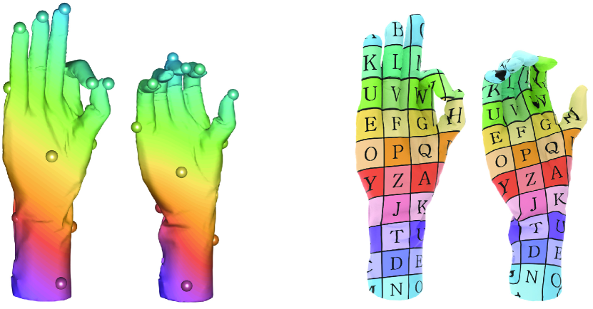
Figure 1. A map between shapes of different genus obtained by our approach. (left) Output landmark correspondence and functional map, visualized using color transfer. (right) Final pointwise map visualized using texture transfer.

We propose to leverage the efficient algorithms for solving the second problem to generate a framework for solving the first. Specifically, we suggest a combinatorial optimization for matching a sparse set of landmarks, such that the best obtainable local distortion of the corresponding sparse-to-dense extension is minimized. As the optimization tool, we propose to use a genetic algorithm, as these have been used for combinatorial optimization for a few decades (Holland, 1992), and are quite general in the type of objectives they can optimize. Despite their success in other fields, though, to the best of our knowledge, their use in shape analysis has been limited so far to isometric matching (Sahillioğlu, 2018).

Using a genetic algorithm allows us to optimize a challenging objective function, that is given both in terms of the landmark permutation and the differential properties of the extended map computed from these landmarks. We use a non-linear non-convex objective, given by the elastic energy of the deformation of the shapes, an approach that has been recently used successfully for non-isometric matching (Ezuz et al., 2019a) when the landmarks are known. Furthermore, we apply the functional map framework (Ovsjanikov et al., 2012) to allow for an efficient computation of the elastic energy. Finally, paramount to the success of a genetic algorithm are the genetic operators, that combine two sparse correspondences to generate a new one, and mutate an existing correspondence. We design novel geometric genetic operators that are guaranteed to yield new valid correspondences. We show that our algorithm yields a landmark correspondence that, when extended to a functional map and a full vertex-to-point map, outperforms existing state-of-the-art techniques for automatic shape correspondence, both quantitatively and qualitatively.

1.1. Related Work

As the literature on shape correspondence is vast, we discuss here only methods which are directly relevant to our approach. For a more detailed survey on shape correspondence we refer the reader to the excellent reviews (Van Kaick et al., 2011; Tam et al., 2013).

Fully automatic shape correspondence.

Many fully automatic methods, like ours, compute a sparse correspondence between the shapes, to decrease the number of degrees of freedom and possible solutions. A sparse-to-dense method can then be used in a post processing step to obtain a dense map. For example, one of the first of such methods was proposed by Zhang et al. (2008), who used a search tree traversal technique to optimize a deformation energy of sparse landmark correspondence. Later, Kezurer et al. (2015) formulated the shape correspondence problem as a Quadratic Assignment Matching problem, and suggested a convex semi-definite programming (SDP) relaxation to solve it efficiently. While the convex relaxation was essential, their method is still only suitable for small sets (of the same size) of corresponding landmarks. Dym et al. (2017) suggested to combine doubly stochastic and spectral relaxations to optimize the Quadratic Assignment Matching problem, which is not as tight as the SDP relaxation, but much more efficient. Maron et al. (2016) suggested a convex relaxation to optimize a term that relates pointwise and functional maps, which promotes isometries by constraining the functional map to be orthogonal.

Other methods for the automatic computation of a dense map include Blended Intrinsic Maps (BIM) by Kim et al. (2011), who optimized for the most isometric combination of conformal maps. Their method works well for relatively similar shapes and generates locally smooth results, yet is restricted to genus-$0$ surfaces. Vestner et al. (2017) suggested a multi scale approach that is not restricted to isometries, but requires shapes with the same number of vertices and generates a bijective vertex to vertex correspondence.

A different approach to tackle the correspondence problem is to compute a fuzzy map (Ovsjanikov et al., 2012; Solomon et al., 2016). The first approach puts in correspondence functions instead of points, whereas the second is applied to probability distributions. These generalizations allow much more general types of correspondences, e.g. between shapes of different genus, however, they also require an additional pointwise map extraction step. The functional map approach was used and extended by many following methods, for example Nogneng et al. (2017) introduced a pointwise multiplication preservation term, Huang et al. (2017) used the adjoint operators of functional maps, and Ren et al. (2018) recently suggested to incorporate an orientation preserving term and a pointwise extraction method that promotes bijectivity and continuity, that can be used for non isometric matching as well.

Our method differs from most existing methods by the quality measure that we optimize. Specifically, we optimize for the landmark correspondence by measuring the elastic energy of the dense correspondence implied by these landmarks. As we show in the results section, our approach outperforms existing automatic state-of-the-art techniques on challenging datasets.

Semi-automatic shape correspondence.

Many shape correspondence methods use a non-trivial initialization, e.g., a sparse landmark correspondence, to warm start the optimization of a dense correspondence. Panozzo et al. (2013) extended a given landmark correspondence by computing the surface barycentric coordinates of a source point with respect to the landmarks on the source shape, and matching that to target points which have similar coordinates with respect to the target landmarks. The landmarks were chosen interactively, thus promoting intuitive user control. More recently, Gehre et al. (2018), used curve constraints and functional maps, for computing correspondences in an interactive setting. Given landmark correspondences or an extrinsic alignment, Mandad et al. (2017) used a soft correspondence, where each source point is matched to a target point with a certain probability, and minimized the variance of this distribution. Parameterization based methods map the two shapes to a single, simple domain, such that the given landmark correspondence is preserved, and the composition of these maps yields the final result (Aigerman et al., 2015; Aigerman and Lipman, 2015, 2016). Since minimizing the distortion of the maps to the common domain does not guarantee minimal distortion of the final map, recently Ezuz et al. (2019b) directly optimized the Dirichlet energy and the reversibility of the forward and backward maps, which led to results with low conformal distortion. Finally, many automatic methods, for example, all the functional map based approaches, can use landmarks as an auxiliary input to improve the results in highly non isometric settings.

The output of our method is a sparse correspondence and a functional map, which can be used as input to semi-automatic methods to generate a dense map. Thus, our approach is complementary to semi-automatic methods. Specifically, we use a recent, publically available method (Ezuz et al., 2019b) to extract a dense vertex-to-point map from the landmarks and functional map that we compute with the genetic algorithm.

Learning based Methods.

Since the correspondence problem can be difficult to model analytically, many machine learning and neural networks based methods, have been suggested. Litman et al. (2014) learn shape descriptors based on their spectral properties. Wei et al. (2016) find the correspondence between humans’ depth maps rendered from multiple viewpoints by computing per-pixel feature descriptors. (Huang et al., 2017) learn a local descriptor from multiple images of the shapes, taken from different angles and scales. Other methods use local isotropic or anisotropic filters in intrinsic convolution layers (Masci et al., 2015; Boscaini et al., 2016; Monti et al., 2017). Lim et al. (2018) presented SpiralNet, performing convolution by a spiral operation for enumerating the information from neighboring vertices. Poulenard and Ovsjanikov (2018) define a multi-directional convolution. Another approach, proposed by Litany et al. (2017), is a network architecture based on functional maps, which was additionally used for unsupervised learning schemes (Halimi et al., 2019; Roufosse et al., 2019).

Genetic algorithms.

Genetic algorithms were initially inspired by the process of evolution and natural selection (Holland, 1992). In the last few decades they have been used in many domains, such as: protein folding simulations (Unger and Moult, 1993), clustering (Maulik and Bandyopadhyay, 2000) and image segmentation (Bhanu et al., 1995), to mention just a few. In the context of graph and shape matching, genetic algorithms were used for registration of depth images (Chow et al., 2004; Silva et al., 2005), 2D shape recognition in images (Ozcan and Mohan, 1997), rigid registration of 3-D curves and surfaces (Yamany et al., 1999), and inexact graph matching (Cross et al., 1997; Auwatanamongkol, 2007).

More recently, Sahillioğlu (2018) suggested a genetic algorithm for isometric shape matching. However, their approach is very different from ours. First, their objective was the preservation of the pairwise distances between the sparse landmarks, which is only appropriate for isometric shapes. We, on the the other hand, use the energy of a dense correspondence, which is the output of a sparse-to-dense algorithm, as our objective. This allows us to match correctly shapes which have large non-isometric deformations. Furthermore, we define novel geometric genetic operators, which are tailored to our problem, and lead to superior results in challenging, highly non-isometric cases. We additionally compare with other state of the art methods for automatic sparse correspondence (Kezurer et al., 2015; Dym et al., 2017; Sahillioğlu, 2018), and with a recent functional map based method (Ren et al., 2018) that automatically computes dense maps and does not have topological restrictions. We apply the same sparse-to-dense post-processing to all methods, and show that we outperform previous methods, as demonstrated by both quantitative and qualitative evaluation.

1.2. Contribution

Our main contributions are:

• A novel use of the functional framework within a genetic pipeline for designing an efficient, geometric objective function that is resilient to non-isometric deformations.

• Novel geometric genetic operators for combining and mutating partial sparse landmark correspondences that are guaranteed to yield valid new correspondences.

• A fully automatic pipeline for matching non-isometric shapes that achieves superior results compared to state-of-the-art automatic methods.

2. Background

2.1. Notation

Meshes.

We compute a correspondence between two manifold triangle meshes, denoted by $M_{1}$ and $M_{2}$. The vertex, edge and face sets are denoted by $\mathcal{V}_{i},\ \mathcal{E}_{i},\ \mathcal{F}_{i}$, respectively, where the subscript $i\!\in\!\{1,2\}$ indicates the corresponding mesh. We additionally denote the number of vertices $|\mathcal{V}_{i}|$ by $n_{i}$. The embedding in $\mathbb{R}^{3}$ of the mesh $M_{i}$ is given by $X_{i}\!\in\!\mathbb{R}^{n_{i}\times 3}$. Given a matrix $A\!\in\!\mathbb{R}^{n\times r}$, we denote its $v$-th row by ${\left[{A}\right]_{{v}\cdot}}\!\in\!\mathbb{R}^{1\times r}$. For example, the embedding in $\mathbb{R}^{3}$ of a vertex $v\!\in\!\mathcal{V}_{i}$ is given by ${\left[{X_{i}}\right]_{{v}\cdot}}\!\in\!\mathbb{R}^{1\times 3}$. The area of a face $f\!\in\!\mathcal{F}_{i}$, and a vertex $v\!\in\!\mathcal{V}_{i}$ are denoted by $a_{f},a_{v}$, respectively. The area of a vertex is defined to be a third of the sum of the areas of its adjacent faces.

Maps.

A pointwise map that assigns a point on $M_{2}$ to each vertex of $M_{1}$ is denoted by $T_{12}:\mathcal{V}_{1}\to M_{2}$. The corresponding functional map matrix that maps piecewise linear functions from $M_{2}$ to $M_{1}$ is denoted by $P_{12}\!\in\!\mathbb{R}^{n_{1}\times n_{2}}$. Similarly, maps in the opposite direction are denoted by swapped subscripts, e.g. $T_{21}$ is a pointwise map from $M_{2}$ to $M_{1}$. The eigenfunctions of the Laplace-Beltrami operator of $M_{i}$ that correspond to the smallest $k_{i}$ eigenvalues are used as a reduced basis for scalar functions, and are stacked as the columns of the basis matrix $\Psi_{i}\!\in\!\mathbb{R}^{n_{i}\times k_{i}}$. A functional map matrix that maps functions in these reduced bases from $M_{2}$ to $M_{1}$ is denoted by $C_{12}\!\in\!\mathbb{R}^{k_{1}\times k_{2}}$.

2.2. Functional Maps

2.2.1. Maps as Composition Operators.

Given a pointwise map $T_{12}$ that maps vertices on $M_{1}$ to points on $M_{2}$, let $X_{12}\!\in\!\mathbb{R}^{n_{1}\times 3}$ denote the embedding coordinates in $\mathbb{R}^{3}$ of the mapped points on $M_{2}$. Now, consider a vertex $v_{1}\!\in\!\mathcal{V}_{1}$ such that $T_{12}(v_{1})$ lies on the triangle $\{u_{2},v_{2},w_{2}\}\!\in\!\mathcal{F}_{2}$, where $u_{2},v_{2},w_{2}\!\in\!\mathcal{V}_{2}$. We can represent the embedding coordinates of $T_{12}(v_{1})$ using barycentric coordinates as ${\left[{X_{12}}\right]_{{v_{1}}\cdot}}=\gamma_{u}{\left[{X_{2}}\right]_{{u_{2}}\cdot}}+\gamma_{v}{\left[{X_{2}}\right]_{{v_{2}}\cdot}}+\gamma_{w}{\left[{X_{2}}\right]_{{w_{2}}\cdot}}\!\in\!\mathbb{R}^{1\times 3}$, where $\gamma_{u},\gamma_{v},\gamma_{w}$ are non-negative and sum to 1. Alternatively, we can write this concisely as ${\left[{X_{12}}\right]_{{v_{1}}\cdot}}=\gamma X_{2}$, where $\gamma\!\in\!\mathbb{R}^{1\times n_{2}}$ is a vector that has all entries zero except at the indices $u_{2},v_{2},w_{2}$, which hold the barycentric coordinates $\gamma_{u},\gamma_{v},\gamma_{w}$, respectively. We repeat this process for all the vertices of $M_{1}$, and build a matrix $P_{12}\!\in\!\mathbb{R}^{n_{1}\times n_{2}}$, such that, for example, ${\left[{P_{12}}\right]_{{v_{1}}\cdot}}=\gamma$. Now, it is easy to check that $X_{12}=P_{12}X_{2}$.

In the same manner that we have applied it to the coordinate functions $X_{2}$, the matrix $P_{12}$ can be used to map any piecewise linear function from $M_{2}$ to $M_{1}$. Specifically, given a piecewise linear function on $M_{2}$, which is given by its values at the vertices $f_{2}\!\in\!\mathbb{R}^{n_{2}\times 1}$, the corresponding function on $M_{1}$ is given by $f_{1}=P_{12}f_{2}\!\in\!\mathbb{R}^{n_{1}\times 1}$. The defining property of $f_{1}$ is that is given by composition, specifically $f_{1}(v_{1})=f_{2}(T_{12}(v_{1}))$, where we extend $f_{2}$ linearly to the interior of the faces. Thus, $P_{12}f_{2}=f_{2}\circ T_{12}$.

The idea of using composition operators, denoted as functional maps, to represent maps between surfaces, was first introduced by Ovsjanikov et al. (2012; 2016). Note that, on triangle meshes, if $T_{12}$ is given, $P_{12}$ is defined uniquely, using the barycentric coordinates construction that we have described earlier. If, on the other hand, $P_{12}$ is given, and it has a valid sparsity structure and values, then it also uniquely defines the map $T_{12}$. This holds, since the non-zero indices in ${\left[{P_{12}}\right]_{{v_{1}}\cdot}}$ indicate on which triangle of the target surface $T_{12}(v_{1})$ lies, and the non-zero values indicate the barycentric coordinates of the mapped point in that triangle.

Working with the matrices $P_{12}$ instead of the pointwise maps $T_{12}$ has various advantages (Ovsjanikov et al., 2016). One of them is that instead of working with the full basis of piecewise linear functions, one can work in a reduced basis $\Psi_{i}$ of size $k_{i}$. By conjugating $P_{12}$ with the reduced bases, we get a compact functional map:

(1) $$C(P_{12})=C_{12}=\Psi_{1}^{\dagger}P_{12}\Psi_{2}\in\mathbb{R}^{k_{1}\times k_{2}}.$$

The small sized matrix $C_{12}$ is easier to optimize for than the full matrix $P_{12}$. Furthermore, for simplicity, the structural constraints on $P_{12}$ are not enforced when optimizing for $C_{12}$, leading to unconstrained optimization problems with a small number of variables. Conversely, once a small matrix $C_{12}$ is extracted, a full matrix $P_{12}$ is often reconstructed and converted to a pointwise map $T_{12}$ for downstream use in applications. The reconstruction is not unique (see, e.g., the discussion by Ezuz et al. (2017)), and in this paper we will use:

(2) $$P(C_{12})=P_{12}=\Psi_{1}C_{12}\Psi_{2}^{\dagger}\in\mathbb{R}^{n_{1}\times n_{2}}.$$

Note that $P(C_{12})$ does not, in general, have the required structure to represent a pointwise map $T_{12}$. We will address this issue further in following sections.

2.2.2. Basis.

The first $k_{i}$ eigenfunctions of the Laplace-Beltrami (LB) operator of $M_{i}$ are often used as the reduced basis $\Psi_{i}$, such that smooth functions are well approximated using a small number of coefficients and $C_{12}$ is compact.

It is often valuable to use a larger basis size for the target functions, so that mapped functions are well represented. Hence, since $C_{ij}$ maps functions on $M_{j}$ to functions on $M_{i}$, $\Psi_{i}$ should contain more basis functions than $\Psi_{j}$. Thus, we denote the number of source eigenfunctions by $k_{s}$, the number of target eigenfunctions by $k_{t}$, and the functional maps in both directions $C_{12},C_{21}$are of size $k_{t}\times k_{s}$. Slightly abusing notations, and to avoid clutter, we use $\Psi_{i}$ to denote the eigenfunctions corresponding to $M_{i}$, in both directions, namely both when $k_{i}=k_{s}$ and $k_{i}=k_{t}$, as the meaning is often clear from the context. Where required, we will explicitly denote by $\Psi_{i_{s}},\Psi_{i_{t}}$ the eigenfunctions with dimensions $k_{s},k_{t}$, respectively. For example, $C(P_{12})=C_{1_{t}2_{s}}=\Psi_{1_{t}}^{\dagger}P_{12}\Psi_{2_{s}}\!\in\!\mathbb{R}^{k_{t}\times k_{s}}$, and similarly for $P(C_{12})$.

2.2.3. Objectives.

Many cost functions have been suggested for functional map computation, e.g., (Ovsjanikov et al., 2012; Nogneng and Ovsjanikov, 2017; Cheng et al., 2018; Ren et al., 2018), among others. In our approach we use the following terms.

Landmark correspondence.

Given a set $\Pi$ of pairs of corresponding landmarks, $\Pi=\{(i,j)\,|\,i\in\mathcal{V}_{1},j\in\mathcal{V}_{2}\}$, we use the term:

(3) $$\mathcal{E}^{m}\left(C_{12},\Pi\right)=\sum_{\left(i,j\right)\in\Pi}\|{\left[{\Psi_{1}}\right]_{{i}\cdot}}C_{12}-{\left[{\Psi_{2}}\right]_{{j}\cdot}}\|^{2}.$$

While some methods use landmark-based descriptors, we prefer to avoid it due to possible bias towards isometry that might be inherent in the descriptors. The formulation in Equation (3) has been used successfully by Gehre et al. (Gehre et al., 2018) for functional map computation between highly non isometric shapes, as well as in the context of pointwise map recovery (Ezuz and Ben-Chen, 2017).

Commutativity with Laplace-Beltrami.

We use:

(4) $$\mathcal{E}^{\Delta}\left(C_{12}\right)=\|\Delta_{1}C_{12}-C_{12}\Delta_{2}\|_{F}^{2},$$

where $\Delta_{i}$ is a diagonal matrix holding the first $k_{i}$ eigenvalues of the Laplace-Beltrami operator of $M_{i}$. While initially this term was derived to promote isometries, in practice it has proven to be useful for highly non isometric shape matching as well (Gehre et al., 2018).

To compute a functional map $C_{12}$ from a set $\Pi$ of pairs of corresponding landmarks, we optimize the following combined objective:

(5) $$\mathcal{E}^{\text{map}}(C_{12},\Pi)=\alpha\,\mathcal{E}^{\Delta}(C_{12})+\beta\,\mathcal{E}^{m}(C_{12},\Pi).$$

2.3. Elastic Energy

Elastic energies are commonly used for shape deformation (Botsch et al., 2006; Sorkine and Alexa, 2007; Heeren et al., 2012; Heeren et al., 2014), but were used for shape matching as well (Litke et al., 2005; Windheuser et al., 2011; de Buhan et al., 2016; Iglesias et al., 2018; Ezuz et al., 2019a). In this paper we use a recent formulation that achieved state of the art results for non isometric shape matching (Ezuz et al., 2019a). The full details are described there, and we mention here only the main equations for completeness.

The elastic energy is defined for a source undeformed mesh $M$, and a deformed mesh with the same triangulation but different geometry $\tilde{M}$. It consists of two terms, a membrane term and a bending term. The membrane energy penalizes area distortion:

(6) $$\mathcal{E}^{\text{mem}}(M,\tilde{M})=\sum_{t\in\mathcal{F}}a_{t}\left(\frac{1}{2}\mathrm{tr}\mathcal{G}_{t}+\frac{1}{4}\det\mathcal{G}_{t}-\frac{3}{4}\log\det\mathcal{G}_{t}-\frac{5}{4}\right),$$

where $a_{t}$ denotes the area of face $t$, and $\mathcal{G}_{t}$$=\hat{g}_{t}^{-1}g_{t}\in\mathbb{R}^{2\times 2}$ denotes the geometric distortion tensor of the face $t$. Here $\hat{g}_{t},g_{t}$ are the discrete first fundamental forms of $M$ and $\tilde{M}$, respectively. In addition, in order to have a finite expression in case some triangles are deformed into zero area triangles, the negative $\log$ function is linearly extended below a small threshold.

The bending energy, on the other hand, penalizes misalignment of curvature features:

(7) $$\mathcal{E}^{\text{bnd}}(M,\tilde{M})=\sum_{e\in\mathcal{E}}\frac{(\tilde{\theta}_{e}-\theta_{e})^{2}}{\tilde{d}_{e}}\left(\tilde{l}_{e}\right)^{2}\,,$$

where $\theta_{e},\tilde{\theta}_{e}$ denote the dihedral angle at edge $e$ in the undeformed and deformed surfaces respectively; if $t,t^{\prime}$ are the adjacent triangles to $e$ then $\tilde{d}_{e}=\frac{1}{3}(\tilde{a}_{t}+\tilde{a}_{t^{\prime}})$, and $\tilde{l}_{e}$ is the length of $e$ in the deformed surface. To handle degeneracies, we sum only over edges where both adjacent triangles are not degenerate.

The elastic energy is:

(8) $$\mathcal{E}^{\text{elstc}}(M,\tilde{M})=\mu\,\mathcal{E}^{\text{mem}}(M,\tilde{M})+\eta\,\mathcal{E}^{\text{bnd}}(M,\tilde{M})\,,$$

where we always use $\mu=1,\eta=10^{-3}$.

Given a pointwise map $T_{12}:M_{1}\to M_{2}$, we evaluate the induced elastic energy as follows. The undeformed mesh is given by $M_{1}$, and the geometry of the deformed mesh is given by the embedding on $M_{2}$ of the images of the vertices of $M_{1}$. Specifically, these are given by $T_{12}(\mathcal{V}_{1})$, or equivalently, $P_{12}X_{2}$, where $X_{2}$ is the embedding of the vertices of $M_{2}$.

2.4. Energies of Functional Maps

Elastic energy.

The elastic energy can also be used to evaluate functional maps directly, by setting the geometry of the deformed mesh to $P(C_{12})X_{2}$. For brevity, we denote this energy by $\mathcal{E}^{\text{elstc}}\left(C_{12}\right)$.

Reversibility energy.

In (Ezuz et al., 2019a) the elastic energy was symmetrized and combined with a reversibility term that evaluates bijectivity. The reversibility term requires computing both $C_{12}$ and $C_{21}$. Here we define the reversibility energy for functional maps, similarly to (Eynard et al., 2016):

(9) $$\begin{split}\mathcal{E}^{\text{rev}}\left(C_{12},C_{21}\right)=&\|C_{12}\Psi_{2}^{\dagger}P(C_{21})X_{1}-\Psi_{1}^{\dagger}X_{1}\|_{F}^{2}+\\ &\|C_{21}\Psi_{1}^{\dagger}P(C_{12})X_{2}-\Psi_{2}^{\dagger}X_{2}\|_{F}^{2}\ .\end{split}$$

The reversibility energy measures the distance between vertex coordinates (projected on the reduced basis), and their mapping to the other shape and back. The smaller this distance is, the more bijectivity is promoted (Ezuz et al., 2019b).

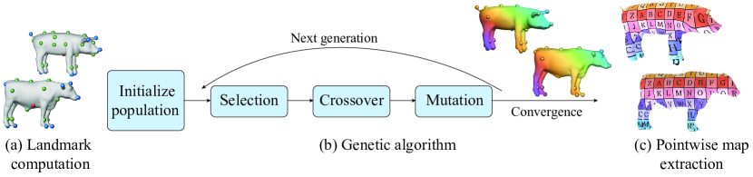
Figure 2. Our pipeline: (a) landmark computation (Section 4), (b) genetic algorithm (Section 5), (c) sparse to dense post processing using (Ezuz et al., 2019b).

3. Method

Our goal is to automatically compute a semantic correspondence between two shapes, denoted by $M_{1}$ and $M_{2}$. The shapes are the only input to our method. We do not assume that the input shapes are isometric, but we do assume that both shapes belong to the same semantic class, so that a semantic correspondence exists. Our pipeline consists of three main steps, see Figure 2:

1. Compute two sets of geometrically meaningful landmarks on $M_{i}$, denoted by $\mathcal{S}_{i}$ (Section 4).

2. Compute a partial sparse correspondence, i.e. a permutation $\Pi$ between subsets of the landmarks $\mathcal{S}^{+}_{i}\subseteq\mathcal{S}_{i}$, as well as corresponding functional maps $C_{ij}$, using a genetic algorithm (Section 5).

3. Generate a dense pointwise map using an existing semi automatic correspondence method (Ezuz et al., 2019b).

We use standard techniques for the first and last steps, and thus our main technical contribution lies in the design of the genetic algorithm.

The most challenging problem is determining the objective function. Unlike the isometric correspondence case, where it is known that pairwise distances between landmarks should be preserved, in the general (not necessarily isometric) case there is no known criterion that the landmarks should satisfy. However, there exist well studied differential quality measures of local distortion, which have proved to be useful in practice for dense non isometric correspondence. Hence, our approach is to find a landmark correspondence that induces the best distortion minimizing map. The general formulation of the optimization problem we address is therefore:

(10) $$\underset{\Pi}{\text{minimize}} \mathcal{E}^{\text{fit}}(C_{\text{opt}}(\Pi))$$

subject to $$C_{\text{opt}}(\Pi)=\underset{C}{\text{argmin}}\,\,\mathcal{E}^{\text{map}}(C,\Pi).$$

Here, $\mathcal{E}^{\text{fit}}$ is a non-linear, non-convex objective, measured on the extension of the landmarks to a full map, and $\mathcal{E}^{\text{map}}$ is the objective used for computing that extension. Thus, the variable in the objective $\mathcal{E}^{\text{fit}}$, i.e. the induced map given by a set of landmarks, is itself the solution of an optimization problem. Hence, two important issues come to light.

First, the importance of using a genetic algorithm, that, in addition to handling combinatorial variables, can be applied to very general objectives. And second, the importance of efficiently evaluating $\mathcal{E}^{\text{fit}}$ and solving the interior optimization problem for the extended map. We achieve this efficiency by using a functional map approach, which performs most computations in a reduced basis, and is thus significantly faster than pointwise approaches.

In the following we discuss the details of the algorithm, first addressing the landmark computation, and then the design of the genetic algorithm that we use to optimize Equation (10). All the parameters are fixed for all the shapes, do not require tuning, and their values are given in the Appendix A.

4. Automatic Landmark Computation

As a pre-processing step, we normalize both meshes to have area $1$. We classify the landmarks into three categories, based on their computation method: maxima, minima, and centers.

Maxima and Minima.

The first two categories are the local maxima and minima of the Average Geodesic Distance (AGD), that is frequently used in the context of landmark computation (Kim et al., 2011; Kezurer et al., 2015). The AGD of a vertex $v\!\in\!\mathcal{V}$ is defined as: $AGD(v)=\sum_{u\in\mathcal{V}}a_{u}d(v,u)$ where $a_{u}$ is the vertex area and $d(v,u)$ is the geodesic distance between $v$ and $u$. To efficiently approximate the geodesic distances, we compute a high dimensional embedding, as suggested by Panozzo et al. (2013), and use the Euclidean distances in the embedding space. The maxima of AGD are typically located at tips of sharp features, and the minima at centers of smooth areas, thus the maxima of the AGD provide the most salient features.

Centers.

As the maxima and minima of the AGD are very sparse, we add additional landmarks using the local minima of the function:

(11) $$f_{N}(v)=\sum_{k\leq N}{\frac{1}{\sqrt{\lambda_{k}}}\frac{\left|\Psi_{k}(v)\right|}{\|\Psi_{k}\|_{L^{\infty}}}}\ \quad v\in\mathcal{V}\,,$$

defined by Cheng et al. (2018), who referred to these minima as centers. Here, $\Psi_{k}$ and $\lambda_{k}$ are the $k^{\text{th}}$ eigenfunction and eigenvalue of the Laplace-Beltrami operator, and $N$ is the number of eigenfunctions. We use the minima of Equation (11) rather than, e.g., farthest point sampling (Kezurer et al., 2015), as the centers tend to be more consistent between non isometric shapes.

Filtering.

Landmarks that are too close provide no additional information, and add unnecessary degrees of freedom. Hence, we filter the computed landmarks so that the minimal distance between the remaining ones is above a small threshold $d_{\epsilon}$. When filtering, we prioritize the landmarks according their salience, namely we prefer maxima of the AGD, then minima and then centers. Finally, if the set of landmarks is larger than a maximal size of $\mu$, we increase $d_{\epsilon}$ automatically to yield less landmarks.

Adjacent landmarks.

We later define genetic operators that take the geometry of the shapes into consideration. To that end, we define two landmarks $l_{i},r_{i}\!\in\!\mathcal{S}_{i}$ to be adjacent if their geodesic distance $d_{i}(l_{i},r_{i})<d_{\text{adj}}$ or if they are neighbors in the geodesic Voronoi diagram of $M_{i}$. The set of adjacent landmarks to $l_{i}$ is denoted by $\mathcal{A}(l_{i})$.

Landmark origins.

The landmark categories are additionally used in the genetic algorithm. Given a landmark $l_{1}\!\in\!\mathcal{S}_{1}$, we denote by $\mathcal{O}(l_{1})\subseteq\mathcal{S}_{2}$ the landmarks on $M_{2}$ from the same category.

The maxima, minima and centers of each shape that remain after filtering form the landmark sets $\mathcal{S}_{1},\mathcal{S}_{2}$. The number of landmarks is denoted by $m_{1},m_{2}$, and is not necessarily the same for $M_{1},M_{2}$.

Figure 2(a) shows example landmark sets, where the color indicates the landmark type: blue for maxima, red for minima and green for centers. As expected, the landmarks do not entirely match, however there exists a substantial subset of landmarks that do match. At this point the landmark correspondence is not known, and it is automatically computed in the next step, using the genetic algorithm.

5. Genetic Non Isometric Maps

Genetic algorithms are known to be effective for solving challenging combinatorial optimization problems with many local minima. In a genetic algorithm (Holland, 1992) solutions are denoted by chromosomes, which are composed of genes. In the initialization step, a collection of chromosomes, known as the initial population is created. The algorithm modifies, or evolves, this population by selecting a random subset for modification, and then combining two chromosomes to generate a new one (crossover), and modifying (mutating) existing chromosomes. The most important part of a genetic algorithm is the objective that is optimized, or the fitness function. The ultimate goal of the genetic algorithm is to find a chromosome, i.e. a solution, with the best fitness value. The general genetic algorithm is described in Algorithm 1.

Genetic algorithms are quite general, as they allow the fitness function to be any type of function of the input chromosome. We leverage this generality to define a fitness function that is itself the result of an optimization problem. We further define the genes, chromosomes, crossover and mutation operators and initialization and selection strategies, in a geometric manner.

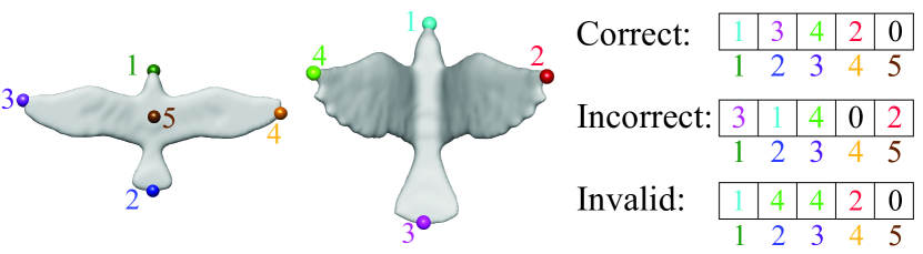
Figure 3. Illustration of chromosomes, which represent a sparse correspondence. The index of an array entry corresponds a landmark of $M_{1}$ (left), and the value corresponds to a landmark on $M_{2}$ (right shape). The first chromosome is the desired semantic correspondence, the second is valid but semantically incorrect, and the third is invalid because it is not injective (landmarks 2,3 on $M_{1}$ correspond to the same landmark 4 on $M_{2}$).

input : $M_{1},M_{2},\mathcal{S}_{1},\mathcal{S}_{2}$

output : $\Pi,C_{\text{opt}}$

Initialize population ;

  // Section 5.2

Evaluate fitness ;

  // Section 5.3

while population did not converge do

       Select individuals for breeding ;

        // Section 5.4

       Perform crossover ;

        // Section 5.5

       Perform mutation ;

        // Section 5.6

       Evaluate offspring fitness and add to population

      

end while

Compute output from fittest chromosome

ALGORITHM 1 Genetic Algorithm.

5.1. Genes and Chromosomes

Genes.

A gene is given by a pair $(l_{1},l_{2})$ such that $l_{1}\!\in\!\mathcal{S}_{1}$ and $l_{2}\!\in\!\mathcal{S}_{2}\cup{0}$, and encodes a single landmark correspondence. If $l_{2}=0$ we denote it as an empty gene, otherwise it is a non-empty gene.

Adjacency Preserving Genes.

Two non-empty genes $(l_{1},l_{2})$ and $(r_{1},r_{2})$ are defined to be adjacency preserving (AP) genes, if $l_{i},r_{i}$ are adjacent landmarks on $M_{i}$, for $i\!\in\!\{1,2\}$.

Chromosome.

A chromosome is a collection of exactly $m_{1}$ genes, that includes a single gene for every landmark in $\mathcal{S}_{1}$. A chromosome is valid if it is injective, namely each landmark on $\mathcal{S}_{2}$ is assigned to at most a single landmark in $\mathcal{S}_{1}$. We represent a chromosome using an integer array of size $m_{1}$, and denote it by $c$, thus the gene $(l_{1},l_{2})$ is encoded by $c[l_{1}]=l_{2}$ (see Figure 3).

Match.

A match defined by a chromosome $c$ is denoted by $\Pi(c)$ and includes all the non-empty genes in $c$. The sets $\mathcal{S}^{+}_{i}(\Pi)\subseteq\mathcal{S}_{i}$ are the landmarks that participate in the genes of $\Pi$, i.e., all the landmarks that have been assigned.

5.2. Initial Population

There are various methods for initialization of genetic algorithms, Paul et al. (2013) discusses and compares different initialization methods of genetic algorithms for the Travelling Salesman Problem, where the chromosome definition is similar to ours. Based on their comparison and the properties of our problem, we use a gene bank (Wei et al., 2007), i.e. for each source landmark we compute a subset of target landmarks that are a potential match.

To compare between landmarks on the two shapes we use a descriptor based distance, the Wave Kernel Signature (WKS) (Aubry et al., 2011). While this choice can induce some isometric bias, as we generate multiple matches for each source landmark, this bias does not affect our results. Let $\mathcal{W}(l_{1},l_{2})$ denote the normalized WKS distance between two landmarks $l_{1}\!\in\!\mathcal{S}_{1},l_{2}\!\in\!\mathcal{S}_{2}$, such that the distance range is $[0,1]$, and is normalized separately for each landmark.

Gene bank.

The gene bank of a landmark $l_{1}\!\in\!\mathcal{S}_{1}$, denoted by $\mathcal{G}(l_{1})$ is the set of genes that match $l_{1}$ to a landmark $l_{2}\!\in\!\mathcal{S}_{2}$ which is close to it in WKS distance, and is of the same origin. Specifically:

(12) $$\mathcal{G}(l_{1})=\,\{(l_{1},l_{2})\,\,| \,\,l_{2}\in\mathcal{O}(l_{1})\,\,\text{\small{and}}$$

$$\,\,\mathcal{W}(l_{1},l_{2})<\epsilon_{\text{wks}}\,\,\text{\small{and}}\,\,\mathcal{W}(l_{2},l_{1})<\epsilon_{\text{wks}}\},$$

The gene bank defines an initial set of possibly similar landmarks. Since it is used for the initialization, the set does not need to be accurate and the WKS distance provides a reasonable initialization even for non-isometric shapes.

Prominent landmark.

A landmark $l_{1}\!\in\!\mathcal{S}_{1}$ is denoted as a prominent landmark if its gene bank $\mathcal{G}(l_{1})$ is not empty, and has at most $4$ genes. This indicates that our confidence in this landmark is relatively high, and we will prefer to start the chromosome building process from such landmarks.

Finally, to add more genes to an existing chromosome, we will need the following definition.

Closest matched/unmatched pair.

Given two disjoint subsets $\mathcal{S}^{+}_{1},\mathcal{S}^{-}_{1}\!\subseteq\!\mathcal{S}_{1}$, we define the closest matched/unmatched pair as the closest adjacent pair, where each landmark belongs to a different subset. In the inset figure, $\mathcal{S}^{+}_{1}$ is displayed in green and $\mathcal{S}^{-}_{1}$ is displayed in blue. The closest matched/unmatched pair $[l^{+}_{1},l^{-}_{1}]$ is circled, $l^{+}_{1}$ in green and $l^{-}_{1}$ in blue. Explicitly:

(13) $$[l^{+}_{1},l^{-}_{1}]=\underset{l_{1}\in\mathcal{S}^{+}_{1},r_{1}\in\mathcal{S}^{-}_{1}}{\text{argmin}}\,\,d_{1}(l_{1},r_{1})\quad\text{s.t.}\quad r_{1}\in\mathcal{A}(l_{1}).$$

5.2.1. Chromosome construction

Using these definitions, we can now address the construction of a new chromosome $c$, as seen in Algorithm 2 and demonstrated in Figure 4.

First, we randomly select a prominent landmark $l_{1}$, and add a random gene from its gene bank $\mathcal{G}(l_{1})$ to $c$. We maintain two subsets $\mathcal{S}^{+}_{1},\mathcal{S}^{-}_{1}\subseteq\mathcal{S}_{1}$, that denote the landmarks that have non-empty genes in $c$, and the unprocessed landmarks, respectively. Hence, initially, $\mathcal{S}^{+}_{1}=\{l_{1}\}$, and $\mathcal{S}^{-}_{1}=\mathcal{S}_{1}\setminus\{l_{1}\}$.

Then, we repeatedly find a closest matching pair $[l^{+}_{1},l^{-}_{1}]$, and try to add an adjacency preserving gene for $l^{-}_{1}$ which keeps the chromosome valid. First, we look for an AP gene in the gene bank $\mathcal{G}(l^{-}_{1})$. If none is found, we try to construct an AP gene $(l^{-}_{1},l_{2})$, where $l_{2}\!\in\!\mathcal{S}_{2}$, and is of the same origin as $l^{-}_{1}$.

If no AP gene can be constructed which maintains the validity of $c$, an empty gene for $l^{-}_{1}$ is added to $c$, and we look for the next closest matching pair. If $\mathcal{A}(\mathcal{S}^{+}_{1})\cap\mathcal{S}^{-}_{1}$ is empty, namely, no more adjacent landmarks remain unmatched, empty genes are added to $c$ for all the remaining landmarks in $\mathcal{S}^{-}_{1}$.

Figure 4 demonstrates the chromosome construction. Both meshes and their computed landmarks (color indicates landmark origin) are displayed in (a). In the first stage, a random prominent landmark is selected, its gene bank (GB) is displayed in magenta on $M_{2}$ (b, top). Then, one random feature is selected from the GB (b, bottom). In the next stage, the closest matched/unmatched pair is selected, and its matching options from the GB are displayed in magenta (c, top). Since only the option from the first chromosome is adjacency preserving (AP), this option is selected (c, bottom). After adding two more landmarks in a similar fashion, the landmark on the chest has a few AP and unselected matching options in the GB (d, top), therefore a random landmark is selected (d, bottom). The next closest unmatched landmark has two matching options (e, top), both are AP, yet the one under the right armpit was previously selected. Therefore the landmark under the left armpit is chosen (e, bottom). After going through all the landmarks, the resulting chromosome is displayed (f, top). After enforcing the match size (see Section 5.2.2), the resulting chromosome is displayed in (f, bottom).

5.2.2. Match size

Given a chromosome $c$, the number of non-empty genes $|\Pi(c)|$ determines how many landmarks are used for computing the dense map. On the one hand, if $|\Pi(c)|$ is too small, it is unlikely that the computed map will be useful. On the other hand, we want to have a variety of possible maps, and thus we require the number of non-empty matches to vary in size.

Hence, before a chromosome is constructed, we randomly select a match size $m_{\min}\leq\tilde{m}\leq m_{\max}$, where $m_{\max}$ is bounded by the landmarks sets’ size $m_{1},m_{2}$, and $m_{\min}$ is a constant fraction of it.

To enforce the match size to be $\tilde{m}$, we discard the constructed chromosome if it does not have enough non-empty genes. If it has too many non-empty genes, we remove genes randomly until we reach the required size. We only remove genes that originate from centers landmarks, as they are often less salient than the other two landmark classes.

5.2.3. Population construction

We construct chromosomes as described previously until completing the initial population or a maximal iteration is reached. During construction, repeated chromosomes are discarded.

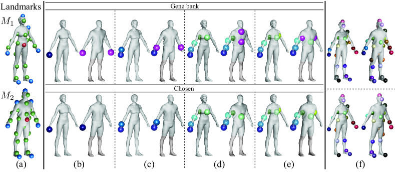
Figure 4. Random chromosome construction. (a) Input landmarks, colored by origin. (b)-(e) iterative addition of genes to the chromosome. The top row shows the landmark on the source, and the gene bank potential matches on the target (in magenta); the bottom row shows the chosen pair of a gene in matching colors. (f) (top) chromosome after adding all the genes and (bottom) after adjusting the match size. See the text for details.

input : Landmark adjacencies $\mathcal{A}$, Landmark origins $\mathcal{O}$

output : A chromosome $c$

Pick a random prominent landmark $l_{1}\in\mathcal{S}_{1}$ ;

  // seed landmark

Add a random gene from $\mathcal{G}(l_{1})$ to $c$ ;

  // first gene from gene bank

$\mathcal{S}^{+}_{1}=\{l_{1}\},\mathcal{S}^{-}_{1}=\mathcal{S}_{1}\setminus\{l_{1}\}$ ;

  // initialize sets

while $\mathcal{A}(\mathcal{S}^{+}_{1})\cap\mathcal{S}^{-}_{1}\neq\emptyset$ do // Adjacent unmatched landmarks exist

       Find closest matched/unmatched pair $[l^{+}_{1},l^{-}_{1}]$

       $g^{+}$ = $(l^{+}_{1},c[l^{+}_{1}])$ ;

        // adjacent gene

       $g$ = pickGene($c,g^{+},l^{-}_{1},\{\mathcal{G}(l^{-}_{1}),\mathcal{O}(l^{-}_{1})\}$) ;

        // gene to add

       add $g$ to $c$

       remove $l^{-}_{1}$ from $\mathcal{S}^{-}_{1}$ ;

        // landmark was processed

       if $g$ is not empty then

             add $l^{-}_{1}$ to $\mathcal{S}^{+}_{1}$

       end if

      

end while

add empty genes for all $l^{-}_{1}\in\mathcal{S}^{-}_{1}$ ;

  // remaining unmatched landmarks

Function pickGene($c,g^{+},l^{-}_{1},\mathcal{S}^{-}_{2}$) is

       foreach $l^{-}_{2}\in\mathcal{S}^{-}_{2}$ do

             $g$ = $(l^{-}_{1},l^{-}_{2})$

             if $g$ is AP to $g^{+}$ and $c\cup g$ is valid then

                   return $g$

                  

             end if

            

       end foreach

      return empty gene

      

end

ALGORITHM 2 Create a random chromosome.

5.3. Fitness

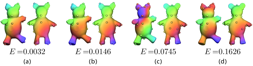
Figure 5. The reversible elastic energy of a few chromosomes. (a) The correct match, (b) the legs are switched, (c) the head and legs are switched (d) an incorrect match. Note that the enetgy gradually increases as more landmarks are mapped incorrectly.

The fitness of a chromosome $c$ is evaluated by extracting a functional map from its match $\Pi(c)$, and evaluating its fitness energy. The fittest chormosome is the one with the lowest fitness energy.

Functional map optimization.

The match $\Pi(c)$ defines a permutation that maps the subset $\mathcal{S}^{+}_{1}$ to $\mathcal{S}^{+}_{2}$ and vice versa. Thus we use it to compute functional maps in both directions, by optimizing

(14) $$\hat{C}_{ij}(\Pi(c))=\underset{C_{ij}}{\text{argmin}}\,\,\mathcal{E}^{\text{map}}(C_{ij},\Pi(c)),$$

where $(i,j)\!\in\!\{(1,2),(2,1)\}$ and $\mathcal{E}^{\text{map}}$ is given in Equation (5). This computation is very efficient, as these are two unconstrained linear least squares problems.

Functional map refinement.

The optimized functional maps $\hat{C}_{ij}$ are efficiently refined by converting them to pointwise maps and back, such that they better represent valid pointwise maps. We solve:

(15) $${P}_{ij}(\hat{C}_{ij})=\underset{P}{\text{argmin}}\,\,\|PX_{j}-P(\hat{C}_{ij})X_{j}\|^{2}_{F},$$

where $P$ is a binary row-stochastic matrix, and $P(C_{ij})$ is given in Equation (2). This problem can be solved efficiently using a $kd$-tree, by finding nearest neighbors in $\mathbb{R}^{3}$. Finally, the optimal functional maps in both directions are given by: $C_{ij}^{\,\text{opt}}=C(P_{ij})$, where $C(P_{ij})$ is given in Equation (1).

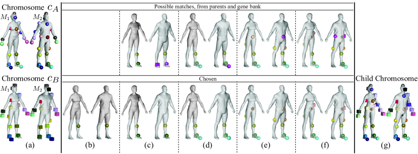
Figure 6. The crossover of two chromosomes $c_{A},c_{B}$ (a) yields a new child chromosome (g). (b-f) the top row shows in each step the potential genes on the target (magenta) with a landmark on the source, and the bottom row shows the chosen genes. (b) initial seed from $c_{A}$, (c) closest unmatched landmark, gene chosen by adjacency, (d) only one potential gene, (e) no potential genes from parents, gene picked from gene bank (marked with $\$$). (f) gene chosen by adjacency. Note that $c_{A}$ switches the hands, $c_{B}$ switches the legs, and the child chromosome matches both correctly.

Functional map fitness.

Finally, we evaluate the fitness of the maps with the reversible elastic energy:

(16) $$\mathcal{E}^{\text{fit}}(C_{12}^{\,\text{opt}},C_{21}^{\,\text{opt}})=\gamma\sum_{ij}\mathcal{E}^{\text{elstc}}(C_{ij}^{\,\text{opt}})+(1-\gamma)\,\mathcal{E}^{\text{rev}}(C_{12}^{\,\text{opt}},\ C_{21}^{\,\text{opt}}),$$

where $\mathcal{E}^{\text{elstc}},\ \mathcal{E}^{\text{rev}}$ are defined in Equations (8) and (9), respectively. While this objective is highly non-linear and non-convex, the fitness is never optimized directly, but only evaluated during the genetic algorithm, which is well suited for such complex objective functions. Figure 5 demonstrates the behavior of the fitness function for a few chromosomes. The sparse correspondences and the resulting functional maps of four chromosomes are displayed. The reversible elastic energy of the correct match is the lowest (a), while a small change such as switching only the legs (b) results in a higher energy. When all the landmarks are mapped incorrectly yet in a consistent way as in (c), where the head and legs are reversed, the energy is even higher, and the highest energy is obtained when the landmarks are mapped incorrectly and inconsistently (d).

5.4. Selection

In this process, individuals from the population are selected in order to pass their genes to the next generation. At each stage half of the population is selected to mate and create offsprings. In order to select the individuals for mating we use a fitness proportionate selection (Back, 1996). In our case the probability to select an individual for mating is proportional to $1$ over its fitness, so that fitter individuals have a better chance of being selected.

input : Landmark adjacencies $\mathcal{A}$, chromosomes $c_{A},c_{B}$

output : Chromosomes $\bar{c}_{A},\bar{c}_{B}$

$\mathcal{S}^{+}_{1A}=\mathcal{S}^{+}_{1}(\Pi(c_{A})),\,\mathcal{S}^{+}_{1B}=\mathcal{S}^{+}_{1}(\Pi(c_{B}))$

$p(\bar{c}_{A})=c_{A},\,p(\bar{c}_{B})=c_{B}$ ;

  // set parents

Pick a random landmark $l_{1}\in\mathcal{S}^{+}_{1A}\cap\mathcal{S}^{+}_{1B}$ ;

  // seed landmark

foreach $\bar{c}\in\{\bar{c}_{A},\bar{c}_{B}\}$ do

       Copy the $l_{1}$ gene from $p(\bar{c})$ to $\bar{c}$ ;

        // first gene

       $\mathcal{S}^{+}_{1}=\{l_{1}\},\mathcal{S}^{-}_{1}=\mathcal{S}_{1}\setminus\{l_{1}\}$ ;

        // initialize sets

       while $\mathcal{S}^{-}_{1}\neq\emptyset$ do // unmatched landmarks exist

             if $\mathcal{A}(\mathcal{S}^{+}_{1})\cap\mathcal{S}^{-}_{1}\neq\emptyset$ then // Adjacent landmarks exist

                   Find closest matched/unmatched pair $[l^{+}_{1},l^{-}_{1}]$

                   $g^{+}$ = $(l^{+}_{1},\bar{c}[l^{+}_{1}])$ ;

                    // adjacent gene

                   $\mathcal{P}$ = $\{(l^{-}_{1},c_{A}[l^{-}_{1}]),(l^{-}_{1},c_{B}[l^{-}_{1}])\}$ ;

                    // parent genes

                   $g$ = pickGene($\bar{c},g^{+},l^{-}_{1},\{\mathcal{P},\mathcal{G}(l^{-}_{1})\}$) ;

                    // gene to add

                  

            else

                   $g$ = random gene from $\Pi(p(\bar{c}))$ such that $\bar{c}\cup g$ is valid

                   if $g=\emptyset$ then // no more parent genes

                         break

                        

                   end if

                  $l^{-}_{1}$ = source landmark of $g$

                  

             end if

            add $g$ to $\bar{c}$

             remove $l^{-}_{1}$ from $\mathcal{S}^{-}_{1}$ ;

              // landmark was processed

             if $g$ is not empty then

                   add $l^{-}_{1}$ to $\mathcal{S}^{+}_{1}$

             end if

            

       end while

      

end foreach

add empty genes for all $l^{-}_{1}\in\mathcal{S}^{-}_{1}$ ;

  // remaining unmatched landmarks

ALGORITHM 3 Crossover.

5.5. Crossover

The chromosomes selected for the next generation undergo a crossover operation with probability $p_{cross}$. The crossover operator merges two input chromosomes $c_{A},c_{B}$ into two new chromosomes $\bar{c}_{A},\bar{c}_{B}$. To combine the input chromosomes in a geometrically consistent way, we again use adjacency preserving (AP) genes, as defined in Section 5.1. The algorithm is similar to the initial chromosome creation, however, rather than matching landmarks based on the gene bank alone, matching is mainly based on the parent chromosomes.

The crossover algorithm is described in Algorithm 3. First, we randomly pick a non empty gene from the parent chromosomes. The correspondence of the selected gene as assigned by $c_{A}$ is the seed of $\bar{c}_{A}$, and correspondence of the same gene as assigned by $c_{B}$ is the seed of $\bar{c}_{B}$. Then, each chromosome is constructed by iteratively adding valid AP genes from the parents. If all the AP genes invalidate the child chromosome, we consider the gene bank options instead, and if these are not valid as well, we pick a random gene that does not invalidate the child chromosome.

Figure 6 demonstrates the creation of $\bar{c}_{A}$ from the parent chromosomes shown in (a). We show corresponding landmarks in the same color, and potential assignments (from the parents or from the gene bank) in magenta. The shape of the landmark (sphere or cube) indicates the parent chromosome.

First, a random non empty gene is copied from $c_{A}$ (b). Then, the closest unmatched landmark is selected (we show the potential genes of both parents) (c, top). Since only the gene of $c_{A}$ is AP, this gene is selected (c, bottom). In (d), the next closest unmatched landmark has only one potential gene, since only $c_{A}$ has a non empty gene with this landmark. Since this option is AP and does not invalidate the chromosome, it is selected. After matching a few more landmarks, a landmark on the stomach is chosen (e, top). This landmark has no potential genes from the parents, therefore, the potential genes are taken from the gene bank (marked with $\$$). In this case there are two possible matching options, one is visible on the stomach, and another is on the back of $M_{2}$ and is not visible in the figure. Both options are AP and do not invalidate the chromosome, so one is chosen randomly (e, bottom). The next closest unmatched landmark has two potential genes (f, top). Both are AP and valid, therefore, one is selected randomly (f, bottom).

After repeating this process for all source landmarks, the resulting chromosome is shown (g). $c_{A}$ maps the legs correctly, yet the arms are switched, whereas $c_{B}$ switches the legs but correctly matches the arms. The child chromosome is, however, better then both its parents, since both the legs and the hands are mapped correctly.

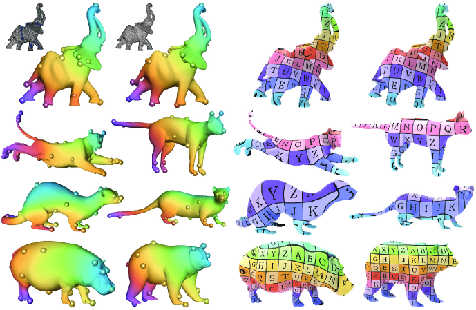
Figure 7. Some qualitative results of our algorithm on meshes of different genus (top), and non isometric shapes (center, bottom).

5.6. Mutation

A new chromosome $c$ can undergo three types of mutations, with some mutation-dependent probability. We define the following mutation operators (Brie and Morignot, 2005).

5.6.1. Growth (probability $p_{grow}$).

Go over all the empty genes in random order and try to replace one, $(l_{1},0)$, by assigning it a corresponding landmark using the following two options.

FMap.

Compute $P_{12}(\hat{C}_{12}(\Pi(c)))$, using equations (14) and (15) and set $l_{2}$ to the closet landmark on $M_{2}$ to $P_{12}(l_{1})$. Add $g=(l_{1},l_{2})$ to $c$ if $c\cup g$ is valid.

Gene Bank.

If the previous attempt failed, set $g$ to a random gene from the gene bank $\mathcal{G}(l_{1})$, and add it to $c$ if $c\cup g$ is valid.

5.6.2. Shrinkage (probability $p_{shrink}$).

Randomly select $n_{\text{sh}}$ centers landmarks from $\mathcal{S}^{+}_{1}(\Pi(c))$. Replace each one of the corresponding genes with an empty gene, such that $n_{\text{sh}}$ new chromosomes are obtained. Each of these has a single new empty gene. The result is the fittest chromosome among them (including the original).

5.6.3. FMap guidance (probability $p_{FMguid}$).

Using equations (14) and (15), compute $P_{12}(\hat{C}_{12}(\Pi(c)))$. For each landmark $l_{1}\!\in\!\mathcal{S}^{+}_{1}(\Pi(c))$ set $l_{2}$ to the closet landmark on $M_{2}$ to $P_{12}(l_{1})$. If injectivity is violated, i.e. $c[i]=c[j]$, if $i$ is a center and $j$ is in another category, set $c[i]=0$ and $c[j]$ as computed by the functional map guidance. Otherwise, randomly keep one of them and set the other one to 0. We prioritize maxima and minima as they are often more salient.

5.7. Stopping criterion

We stop the iterations when the fittest chromosome remains unchanged for a set amount of iterations, meaning the population has converged, or when a maximal iteration number is reached.

5.8. Limitations

We evaluate the quality of a sparse correspondence using the elastic energy of the induced functional map, which is represented in a reduced basis. In some cases, the reduced basis does not contain enough functions to represent correctly the geometry of thin parts of the shape, and as a result both correct and incorrect sparse correspondences can lead to a low value for the elastic energy. Such an example is shown in the inset Figure. Both the body and the legs of the ants are very thin, and the resulting best match switches between the two back legs.

5.9. Timing

The most computationally expensive part of the algorithm is computing the fitness of each chromosome. While computing the functional map and evaluating the elastic energy of one chromosome is fast, this computation is done for all the offspring in each iteration, and is therefore expensive. Our method is implemented in MATLAB. On a desktop machine with an Intel Core i7 processor, for meshes with $5$K vertices, computation of a functional map for a single chromosome takes $0.035$ seconds and the computation of the elastic energy takes $0.002$ seconds. The average amount of iterations it took for the algorithm to converge is $225$ and the average total computation time is $10.5$ minutes.

6. Results

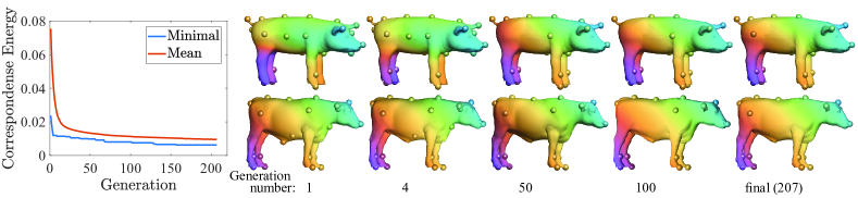
Figure 8. Population evolution. (left) The energy of the fittest offspring and the mean energy of the population decrease until convergence indicating improvement throughout the generations. (right) The fittest offspring at different generations, improving until reaching the correct correspondence.

6.1. Datasets and Evaluation

Our method computes a sparse correspondence and a functional map that can be used as input to existing semi-automatic methods such as (Ezuz et al., 2019b), that we use in this paper.

Datasets.

We demonstrate the results of our method on two datasets with different properties. The SHREC’07 dataset (Giorgi et al., 2007) contains a variety of non-isometric shapes as well as ground truth sparse correspondence between manually selected landmarks. This dataset is suitable to demonstrate the advantages of our method, since we address the highly non-isometric case. The recent dataset SHREC’19 (Dyke et al., 2019) contains shapes of the same semantic class but different topologies, that we use to demonstrate our results in such challenging cases.

Quantitative evaluation.

Quantitatively evaluating sparse correspondence on these datasets is challenging, since the given sparse ground truth does not necessarily coincide with the computed landmarks. We therefore quantitatively evaluate the results after post processing, where we use the same post processing for all methods (if a method produces sparse correspondence we compute functional maps using these landmarks and run RHM (Ezuz et al., 2019b) to extract a pointwise map, and if a method produces a pointwise map we apply RHM directly). Since we initialize RHM with a functional map or a dense map, we use the Euclidean rather than the geodesic embedding that was used in their paper, that is only needed when the initialization is very coarse. We use the evaluation protocol suggested by Kim et al. (2011), where the $x$ axis is a geodesic distance between a ground truth correspondence and a computed correspondence, and the $y$ axis is the percentage of correspondences with less than $x$ error. We also allow symmetries, as suggested by Kim et al. (2011), by computing the error w.r.t. both the ground truth correspondence and the symmetric map (that is given), and using the map with the lower error as ground truth for comparison.

Qualitative evaluation.

We qualitatively evaluate our results using color and texture transfer. We visualize a sparse correspondence by showing corresponding landmarks in the same color. To visualize functional maps we show a smooth function, visualized by color coding on the target mesh, and transfer it to the source using the functional map. We visualize pointwise maps by texture transfer. Figure 7 demonstrates a few examples of our results using these visualizations.

6.2. Population Evolution and Convergence

Figure 8 shows the evolution of the population in the pig-cow example. We plot the mean energy of a chromosome as a function of the generation, as well as the minimal energy (of the fittest chromosome). We also visualize the functional map and the landmarks of the fittest chromosome throughout the algorithm, which is inaccurate at the first iteration (the front legs are matched incorrectly), and gets increasingly more accurate as the population evolves.

We additionally plot the energy of the best chromosome as a function of the generation number for additional shapes in Figure 9. Similarly to the pig-cow example, the energy decreases until the algorithm converges.

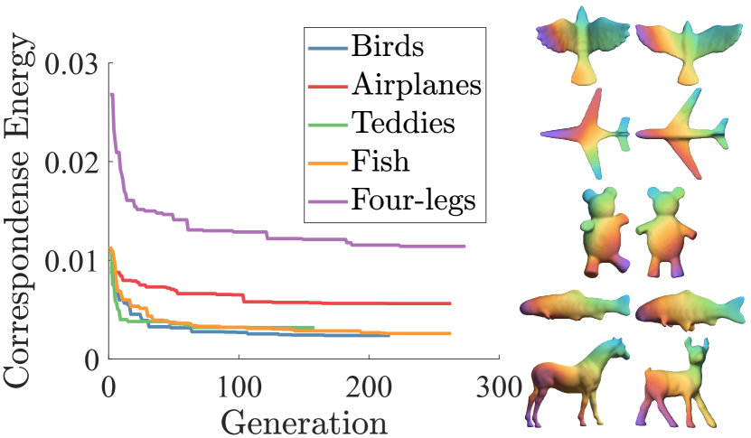
Figure 9. The correspondence energy of the fittest offspring during the iterations (left) and the final map generated from the fittest offspring in the final iteration (right) on a few pairs of shapes. Note that the energy decreases until convergence.

Since our algorithm is not deterministic, we investigate the variation of our results by running the algorithm $100$ times on 20 random pairs of shapes from the SHREC’07 dataset (Giorgi et al., 2007). We evaluate the result using the protocol suggested by Kim et al. (2011), after post processing (Ezuz et al., 2019b) to extract a dense map. The results are determined by the total geodesic error with respect to the sparse ground truth and are shown in the inset Figure. The best and worst results are composed of the best and worst results of each one of the 20 pairs respectively. Note that the total results (all 100 results on all the pairs) are close to the best results, indicating that the worst results are outliers.

6.3. Mapping between Shapes of Different Genus

Our method is applicable to shapes of any genus, and can also match between shapes of different topology. Figure 1 shows our results for two hand models from SHREC’19 (Dyke et al., 2019). The left model has genus $2$ and the right model has genus $1$. Note that our approach yields a high quality dense correspondence even for such difficult cases. We additionally show in Figure 10 our results for two cup models from SHREC’07 (Giorgi et al., 2007), both genus $1$, and two pairs of human shapes with genus $0$ and genus $1$, respectively. Here as well, despite the difficult topological issues, our approach computed a meaningful map. Another example appears in Figure 7 (top). Here, we generated a genus $8$ mesh (left) by introducing tunnels through a genus $3$ mesh (right). Both meshes were then remeshed to have different triangulations. Note that even for meshes with large differences in genus, our method generates good results.

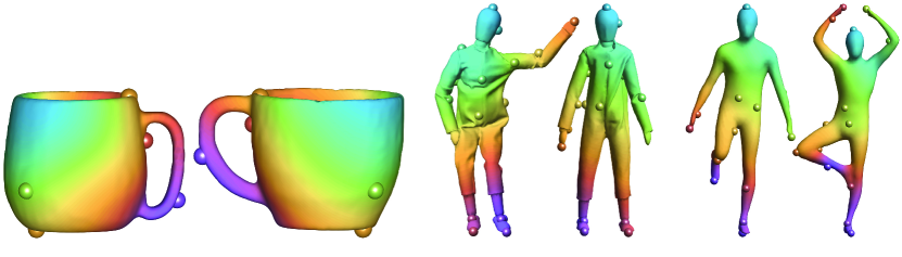
Figure 10. Our results on shapes of genus 1 (top) and shapes with different genus (bottom).

6.4. Evaluation on increasingly non-isometric shapes.

To demonstrate the efficiency of our algorithm on non-isometric shapes, we perform the following experiment. Starting from nearly isometric shapes from the SHREC’07 dataset (Giorgi et al., 2007), we deform one of the shapes (extend the bears’ arm) gradually and obtain $5$ pairs with different degrees of isometric distortion (Figure 11). For the first $5$ pairs (a-e) we find the correct match despite the large deformation, whereas for the last pair (f), where the non-isometric deformation is very high, our algorithm does not find a correct map.

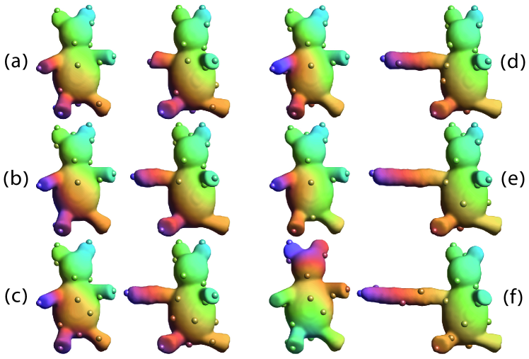
Figure 11. Varying degrees of isometry, from nearly isometric (a) to highly non isometric shapes (f). Our method finds the correct map for most pairs (a-e), yet matches incorrectly the pair with the highest distortion (f).

6.5. Ablation study.

We perform an ablation study to show the effect of different design choices of our algorithm. We run our algorithm $5$ times on $20$ random pairs from the SHREC’07 dataset (Giorgi et al., 2007), where each time one part of the method changes while the rest remains identical. In our first experiment, we use only the maxima and minima as landmarks, removing the centers. Next, we use a random population initialization (Paul et al., 2013), change the fitness to the reversible harmonic energy (Ezuz et al., 2019b) of the functional map extracted from a chromosome, use the cycle crossover (CX) from the traveling salesman problem (Oliver et al., 1987), and finally remove the shrinkage mutation. We evaluate the results as in the previous sections and they are shown in the inset Figure. Note that changing parts of the algorithm diminishes the performance.

6.6. Quantitative and Qualitative Comparisons

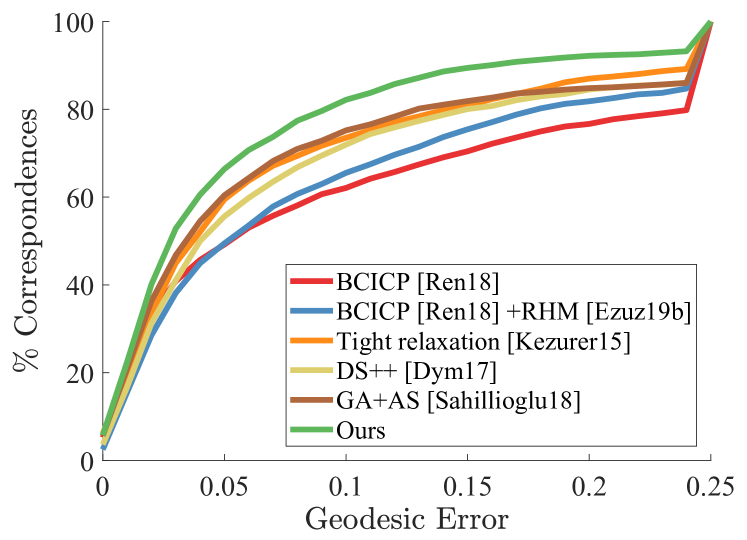
Figure 12. Quantitative comparison between our results and fully automatic state of the art methods (Kezurer et al., 2015; Dym et al., 2017; Sahillioğlu, 2018; Ren et al., 2018). We apply the same post processing (Ezuz et al., 2019b) on all the methods to extract a dense map, and use the evaluation protocol suggested by Kim et al. (2011), that measures geodesic distance to the ground truth. Note that we outperform all the other methods.

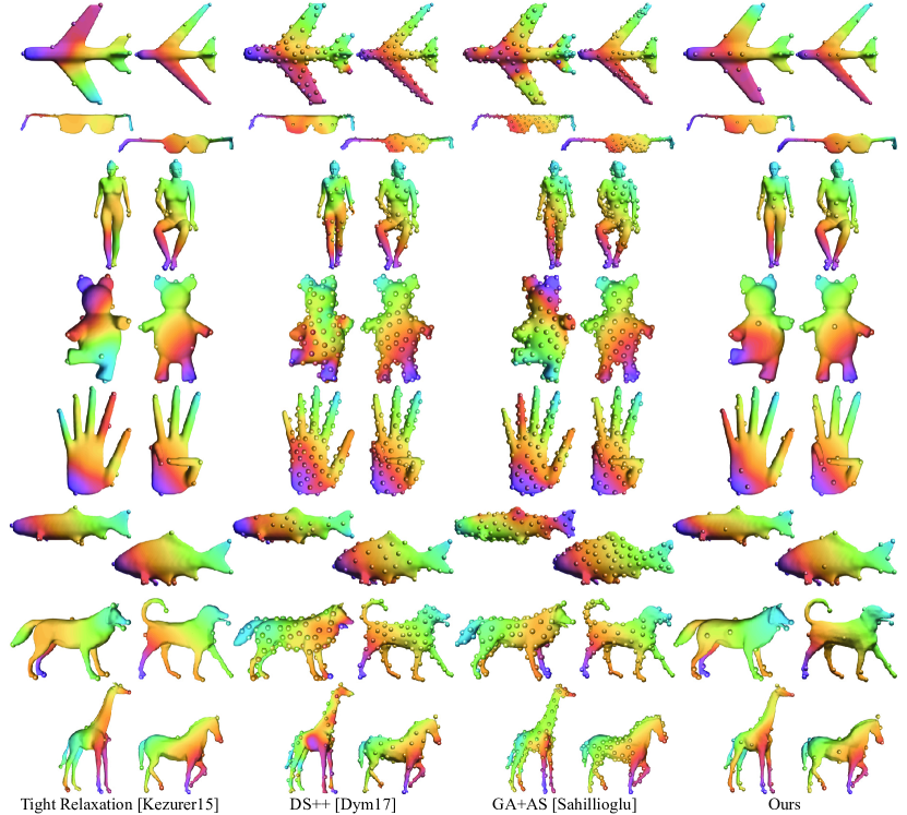
Figure 13. Qualitative comparison between the results of our genetic algorithm, i.e. a sparse correspondence and a functional map, and the results of automatic state of the art methods (Kezurer et al., 2015; Dym et al., 2017; Sahillioğlu, 2018) for sparse correspondence. The functional map is visualized by color transfer (see text for details), and the sparse correspondence is visualized by landmarks with corresponding colors.

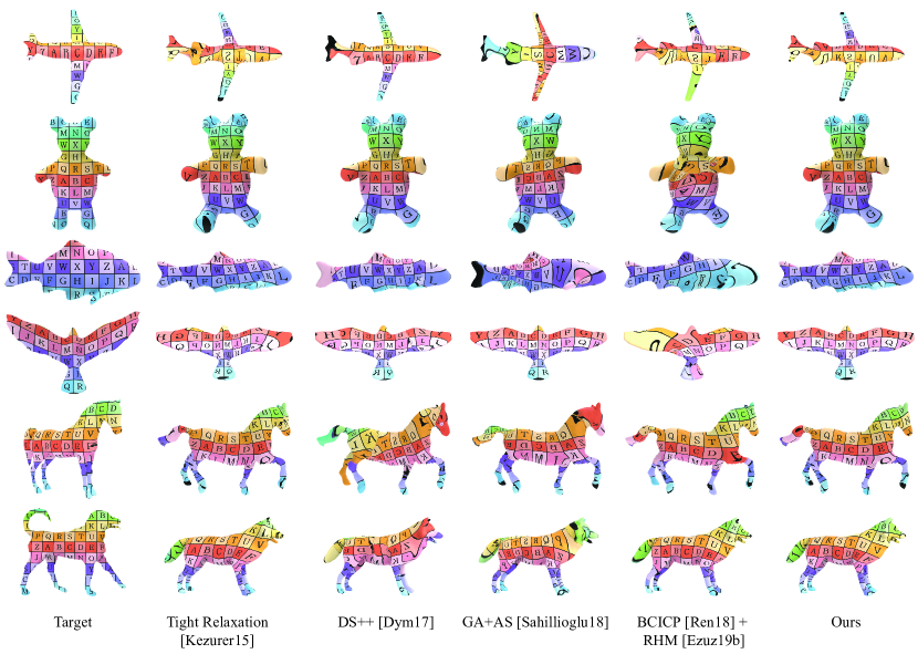
Figure 14. Qualitative comparison between our final results and fully automatic state of the art methods (Kezurer et al., 2015; Dym et al., 2017; Sahillioğlu, 2018; Ren et al., 2018) (after applying the same post processing (Ezuz et al., 2019b) on all the methods to extract a dense map). The pointwise maps are visualized using texture that is computed on the target mesh (left) and transferred to the source using each method.

We compare our method with state of the art methods for sparse and dense correspondence. We only compare with fully automatic methods, since semi automatic methods require additional user input, which is often not available. For comparisons that require a dense correspondence we apply the same post processing for all methods: we compute a functional map as described in section 5.3 and use it as input to the sparse-to-dense post processing method (Ezuz et al., 2019b). We compare the resulting dense pointwise maps quantitatively using the protocol suggested by Kim et al. (2011) as described in section 6.1.

The sparse correspondence methods we compare with are: "Tight Relaxation" by Kezurer et al. (2015), DS++ by Dym et al. (2017), and the recent method by Sahillioglu et al. (2018) that also uses a genetic algorithm (GA+AS, AS stands for Adaptive Sampling which they use for improved results). We additionally compare with the recent dense correspondence method by Ren et al. (2018) (BCICP). Since Ren et al. (2018) computes vertex-to-vertex maps, we apply the post processing (Ezuz et al., 2019b) on their results as well (BCICP+RHM).

The quantitative results are shown in Figure 12, and it is evident that our method outperforms all previous approaches on this highly challenging non-isometric dataset. The sparse correspondence and the functional map are visualized in Figure 13 using the visualization approach described in Section 6.1. Note that our method consistently yields semantic correspondences on shapes from various classes, even in highly non-isometric cases such as the airplanes, the fish and the dog/wolf pair. This is even more evident when examining the texture transfer results in Figure 14, which visualize the dense map. Note the high quality dense map obtained for highly non-isometric meshes such as the fish and the wolf/dog.

We additionally compare our results to those of "Tight Relaxation"  (Kezurer et al., 2015) when matching the same initial landmarks. We generate $15$ landmarks for each shape, following the method used in (Kezurer et al., 2015). As this approach requires the match size as an additional input, we use the values: $11,13$ as well as the match size found automatically by our method as inputs. The results are shown in Figure 15. Note that the match found by our method is correct and outperforms the competing output, whose quality also depends on the requested match size.

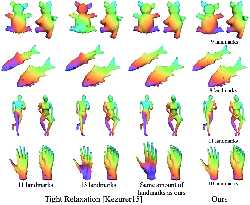
Figure 15. Qualitative comparison with Tight Relaxation (TR)  (Kezurer et al., 2015) using the same $15$ landmarks. (right) Our results, (three left columns) TR results with varying match size: $11,13$ and the size our method found.

7. Conclusion

We present an approach for automatically computing a correspondence between non-isometric shapes of the same semantic class. We leverage a genetic algorithm for the combinatorial optimization of a small set of automatically computed landmarks, and use a fitness energy that is based on extending the sparse landmarks to a functional map. As a result, we achieve high quality dense maps, that outperform existing state-of-the-art automatic methods, and can successfully handle challenging cases where the source and target have a different topology.

We believe that our approach can be generalized in a few ways. First, the decomposition of the automatic mapping computation problem into combinatorial and continuous problems mirrors other tasks in geometry processing which were handled in a similar manner, such as quadrangular remeshing. It is interesting to investigate whether additional analogues exist between these seemingly unrelated problems. Furthermore, it is intriguing to consider what other problems in shape analysis can benefit from genetic algorithms. One potential example is map synchronization for map collections, where the choice of cycles to synchronize is also combinatorial.

Appendix A Parameters

All the parameters are unitless and fixed in all the experiments. We choose the values experimentally, yet our results are not sensitive to these values. Many of the parameters are required by the genetic algorithm and the functional map computations, which both have standard practices.

Centers.

To compute the landmarks classified as centers from Eq.  (11), we use $N=30$ eigenfunctions, as suggested by Cheng et al. (2018).

Filtering.

We filter close landmarks according to the initial distance of $d_{\epsilon}=0.08$, where the distance is on the normalized shape. In addition, we set the maximal amount of landmarks to $\mu=35$. We observed that for a variety of shapes, $35$ landmarks with the specified minimal distance covered the shape features well and gave a large enough subset of matching landmarks for our fitness function.

Adjacent landmarks.

We use the geodesic distance of $d_{\text{adj}}=0.3$ to define adjacent landmarks. This distance is large enough to accommodate highly non-isometric shapes but still allows to construct consistent chromosomes.

Gene bank.

We set the WKS distance to $\epsilon_{\text{wks}}=0.2$.

Match size.

The minimal match size is $m_{\min}=\frac{2}{3}m_{\max}$ and the maximal match size is $m_{\max}=\min(m_{1},m_{2})$ where $m_{i}$ is the number of landmarks on $M_{i}$.

Population construction.

The initial population has $400$ chromosomes, following experiments with varying population sizes and the guidelines by Rylander et al. (2002).

Functional map optimization.

To construct the functional map we use $k_{s}=30,k_{t}=60$ and $\alpha=1$, $\beta=100$, which is standard practice for functional maps computations.

Functional map fitness.

For the elastic energy, we set $\gamma=5\cdot 10^{-4}$ similarly to Ezuz et al. (2019a).

Genetic operators.

For the operators, we use the rates $p_{cross}$$=0.75$, $p_{grow}$$=0.05$ $p_{shrink}$$=0.1$, $p_{FMguid}$$=0.05$. The crossover is the main operator, therefore its rate is much higher than the mutations, as is common for genetic algorithms.

Convergence.

We stop the algorithm if the fittest chromosome remains unchanged for $50$ iterations or when a maximal iteration number of $700$ iterations is reached.

References

- (1)
- Aigerman and Lipman (2015) Noam Aigerman and Yaron Lipman. 2015. Orbifold Tutte Embeddings. ACM TOG 34 (2015).
- Aigerman and Lipman (2016) Noam Aigerman and Yaron Lipman. 2016. Hyperbolic Orbifold Tutte Embeddings. ACM TOG 35 (2016).
- Aigerman et al. (2015) Noam Aigerman, Roi Poranne, and Yaron Lipman. 2015. Seamless surface mappings. ACM TOG 34, 4 (2015), 72.
- Aubry et al. (2011) Mathieu Aubry, Ulrich Schlickewei, and Daniel Cremers. 2011. The Wave Kernel Signature: A Quantum Mechanical Approach to Shape Analysis. In International Conference on Computer Vision Workshops (ICCV Workshops). IEEE.
- Auwatanamongkol (2007) Surapong Auwatanamongkol. 2007. Inexact graph matching using a genetic algorithm for image recognition. Pattern Recognition Letters 28, 12 (2007), 1428–1437.
- Back (1996) Thomas Back. 1996. Evolutionary algorithms in theory and practice: evolution strategies, evolutionary programming, genetic algorithms. Oxford university press.
- Bhanu et al. (1995) Bir Bhanu, Sungkee Lee, and John Ming. 1995. Adaptive image segmentation using a genetic algorithm. IEEE Trans on systems, man, and cybernetics 25, 12 (1995), 1543–1567.
- Boscaini et al. (2016) Davide Boscaini, Jonathan Masci, Emanuele Rodolà, and Michael Bronstein. 2016. Learning shape correspondence with anisotropic convolutional neural networks. In Advances in Neural Information Processing Systems. 3189–3197.
- Botsch et al. (2006) Mario Botsch, Mark Pauly, Markus H Gross, and Leif Kobbelt. 2006. PriMo: coupled prisms for intuitive surface modeling. In Proc. Eurographics SGP. 11–20.
- Brie and Morignot (2005) Alexandru Horia Brie and Philippe Morignot. 2005. Genetic Planning Using Variable Length Chromosomes.. In ICAPS. 320–329.
- Cheng et al. (2018) Xiuyuan Cheng, Gal Mishne, and Stefan Steinerberger. 2018. The geometry of nodal sets and outlier detection. Journal of Number Theory 185 (2018), 48–64.
- Chow et al. (2004) Chi Kin Chow, Hung Tat Tsui, and Tong Lee. 2004. Surface registration using a dynamic genetic algorithm. Pattern recognition 37, 1 (2004), 105–117.
- Cross et al. (1997) Andrew DJ Cross, Richard C Wilson, and Edwin R Hancock. 1997. Inexact graph matching using genetic search. Pattern Recognition 30, 6 (1997), 953–970.
- de Buhan et al. (2016) Maya de Buhan, Charles Dapogny, Pascal Frey, and Chiara Nardoni. 2016. An optimization method for elastic shape matching. C. R. Math. Acad. Sci. Paris 354, 8 (2016), 783–787.
- Dyke et al. (2019) Roberto Dyke, Caleb Stride, Yu-Kun Lai, and Paul L. Rosin. 2019. SHREC 2019. https://shrec19.cs.cf.ac.uk/.
- Dym et al. (2017) Nadav Dym, Haggai Maron, and Yaron Lipman. 2017. DS++: A Flexible, Scalable and Provably Tight Relaxation for Matching Problems. ACM TOG 36, 6 (2017).
- Eynard et al. (2016) Davide Eynard, Emanuele Rodola, Klaus Glashoff, and Michael M Bronstein. 2016. Coupled functional maps. In 2016 Fourth 3DV. IEEE, 399–407.
- Ezuz and Ben-Chen (2017) Danielle Ezuz and Mirela Ben-Chen. 2017. Deblurring and denoising of maps between shapes. In CGF, Vol. 36. Wiley Online Library, 165–174.
- Ezuz et al. (2019a) Danielle Ezuz, Behrend Heeren, Omri Azencot, Martin Rumpf, and Mirela Ben-Chen. 2019a. Elastic Correspondence between Triangle Meshes. In CGF, Vol. 38.
- Ezuz et al. (2019b) Danielle Ezuz, Justin Solomon, and Mirela Ben-Chen. 2019b. Reversible Harmonic Maps between Discrete Surfaces. ACM Transactions on Graphics (2019).
- Ezuz et al. (2017) Danielle Ezuz, Justin Solomon, Vladimir G Kim, and Mirela Ben-Chen. 2017. Gwcnn: A metric alignment layer for deep shape analysis. In CGF, Vol. 36. 49–57.
- Gehre et al. (2018) Anne Gehre, M Bronstein, Leif Kobbelt, and Justin Solomon. 2018. Interactive curve constrained functional maps. In CGF, Vol. 37. Wiley Online Library, 1–12.
- Giorgi et al. (2007) Daniela Giorgi, Silvia Biasotti, and Laura Paraboschi. 2007. SHREC: Shape Retrieval Contest: Watertight Models Track.
- Halimi et al. (2019) Oshri Halimi, Or Litany, Emanuele Rodola, Alex M Bronstein, and Ron Kimmel. 2019. Unsupervised learning of dense shape correspondence. In Proceedings of the IEEE Conference on Computer Vision and Pattern Recognition. 4370–4379.
- Heeren et al. (2014) Behrend Heeren, Martin Rumpf, Peter Schröder, Max Wardetzky, and Benedikt Wirth. 2014. Exploring the Geometry of the Space of Shells. CGF 33, 5 (2014), 247–256.
- Heeren et al. (2012) Behrend Heeren, Martin Rumpf, Max Wardetzky, and Benedikt Wirth. 2012. Time-Discrete Geodesics in the Space of Shells. CGF 31, 5 (2012), 1755–1764.
- Holland (1992) John H Holland. 1992. Genetic algorithms. Scientific american 267, 1 (1992), 66–73.
- Huang et al. (2017) Haibin Huang, Evangelos Kalogerakis, Siddhartha Chaudhuri, Duygu Ceylan, Vladimir G Kim, and Ersin Yumer. 2017. Learning local shape descriptors from part correspondences with multiview convolutional networks. ACM TOG 37, 1 (2017), 1–14.
- Huang and Ovsjanikov (2017) Ruqi Huang and Maks Ovsjanikov. 2017. Adjoint Map Representation for Shape Analysis and Matching. In Computer Graphics Forum, Vol. 36. 151–163.
- Iglesias et al. (2018) José A. Iglesias, Martin Rumpf, and Otmar Scherzer. 2018. Shape-Aware Matching of Implicit Surfaces Based on Thin Shell Energies. Found. Comput. Math. 18, 4 (2018), 891–927.
- Kezurer et al. (2015) Itay Kezurer, Shahar Z Kovalsky, Ronen Basri, and Yaron Lipman. 2015. Tight relaxation of quadratic matching. In Computer Graphics Forum, Vol. 34. 115–128.
- Kim et al. (2011) Vladimir G Kim, Yaron Lipman, and Thomas Funkhouser. 2011. Blended Intrinsic Maps. ACM TOG 30 (2011).
- Lim et al. (2018) Isaak Lim, Alexander Dielen, Marcel Campen, and Leif Kobbelt. 2018. A simple approach to intrinsic correspondence learning on unstructured 3d meshes. In Proceedings of the European Conference on Computer Vision (ECCV). 0–0.
- Litany et al. (2017) Or Litany, Tal Remez, Emanuele Rodolà, Alex Bronstein, and Michael Bronstein. 2017. Deep functional maps: Structured prediction for dense shape correspondence. In Proceedings of the IEEE International Conference on Computer Vision. 5659–5667.
- Litke et al. (2005) Nathan Litke, Mark Droske, Martin Rumpf, and Peter Schröder. 2005. An Image Processing Approach to Surface Matching. In Proc. Eurographics SGP. 207–216.
- Litman and Bronstein (2014) Roee Litman and Alexander Bronstein. 2014. Learning spectral descriptors for deformable shape correspondence. Pattern Analysis and Machine Intelligence, IEEE Transactions on 36, 1 (2014), 171–180.
- Mandad et al. (2017) Manish Mandad, David Cohen-Steiner, Leif Kobbelt, Pierre Alliez, and Mathieu Desbrun. 2017. Variance-Minimizing Transport Plans for Inter-surface Mapping. ACM TOG 36 (2017), 14.
- Maron et al. (2016) Haggai Maron, Nadav Dym, Itay Kezurer, Shahar Kovalsky, and Yaron Lipman. 2016. Point Registration via Efficient Convex Relaxation. ACM TOG 35, 4 (2016).
- Masci et al. (2015) Jonathan Masci, Davide Boscaini, Michael Bronstein, and Pierre Vandergheynst. 2015. Geodesic convolutional neural networks on riemannian manifolds. In The IEEE International Conference on Computer Vision (ICCV). 37–45.
- Maulik and Bandyopadhyay (2000) Ujjwal Maulik and Sanghamitra Bandyopadhyay. 2000. Genetic algorithm-based clustering technique. Pattern recognition 33, 9 (2000), 1455–1465.
- Monti et al. (2017) Federico Monti, Davide Boscaini, Jonathan Masci, Emanuele Rodola, Jan Svoboda, and Michael M Bronstein. 2017. Geometric deep learning on graphs and manifolds using mixture model cnns. In Proceedings of the IEEE Conference on Computer Vision and Pattern Recognition. 5115–5124.
- Munsell et al. (2008) Brent C Munsell, Pahal Dalal, and Song Wang. 2008. Evaluating shape correspondence for statistical shape analysis: A benchmark study. IEEE Transactions on Pattern Analysis and Machine Intelligence 30, 11 (2008), 2023–2039.
- Nogneng and Ovsjanikov (2017) Dorian Nogneng and Maks Ovsjanikov. 2017. Informative descriptor preservation via commutativity for shape matching. In Computer Graphics Forum, Vol. 36. 259–267.
- Oliver et al. (1987) IM Oliver, DJd Smith, and John RC Holland. 1987. Study of permutation crossover operators on the traveling salesman problem. In Genetic algorithms and their applications: proceedings of the second International Conference on Genetic Algorithms: July 28-31, 1987 at the Massachusetts Institute of Technology, Cambridge, MA. Hillsdale, NJ: L. Erlhaum Associates, 1987.
- Ovsjanikov et al. (2012) Maks Ovsjanikov, Mirela Ben-Chen, Justin Solomon, Adrian Butscher, and Leonidas Guibas. 2012. Functional maps: a flexible representation of maps between shapes. ACM TOG 31, 4 (2012).
- Ovsjanikov et al. (2016) Maks Ovsjanikov, Etienne Corman, Michael Bronstein, Emanuele Rodolà, Mirela Ben-Chen, Leonidas Guibas, Frederic Chazal, and Alex Bronstein. 2016. Computing and processing correspondences with functional maps. In SIGGRAPH ASIA 2016 Courses. ACM, 9.
- Ozcan and Mohan (1997) Ender Ozcan and Chilukuri K Mohan. 1997. Partial shape matching using genetic algorithms. Pattern Recognition Letters 18, 10 (1997), 987–992.
- Panozzo et al. (2013) Daniele Panozzo, Ilya Baran, Olga Diamanti, and Olga Sorkine-Hornung. 2013. Weighted averages on surfaces. ACM TOG 32, 4 (2013), 60.
- Paul et al. (2013) P Victer Paul, A Ramalingam, R Baskaran, P Dhavachelvan, K Vivekanandan, R Subramanian, and VSK Venkatachalapathy. 2013. Performance analyses on population seeding techniques for genetic algorithms. International Journal of Engineering and Technology (IJET) 5, 3 (2013), 2993–3000.
- Poulenard and Ovsjanikov (2018) Adrien Poulenard and Maks Ovsjanikov. 2018. Multi-directional geodesic neural networks via equivariant convolution. ACM TOG 37, 6 (2018), 1–14.
- Ren et al. (2018) Jing Ren, Adrien Poulenard, Peter Wonka, and Maks Ovsjanikov. 2018. Continuous and Orientation-preserving Correspondences via Functional Maps. ACM TOG 37, 6 (2018).
- Roufosse et al. (2019) Jean-Michel Roufosse, Abhishek Sharma, and Maks Ovsjanikov. 2019. Unsupervised deep learning for structured shape matching. In Proceedings of the IEEE International Conference on Computer Vision. 1617–1627.
- Rylander and Gotshall (2002) STANLEY GOTSHALL BART Rylander and S Gotshall. 2002. Optimal population size and the genetic algorithm. Population 100, 400 (2002), 900.
- Sahillioğlu (2018) Yusuf Sahillioğlu. 2018. A Genetic Isometric Shape Correspondence Algorithm with Adaptive Sampling. ACM Trans. Graph. 37, 5 (Oct. 2018).
- Silva et al. (2005) Luciano Silva, Olga Regina Pereira Bellon, and Kim L Boyer. 2005. Precision range image registration using a robust surface interpenetration measure and enhanced genetic algorithms. IEEE transactions on pattern analysis and machine intelligence 27, 5 (2005), 762–776.
- Solomon et al. (2016) Justin Solomon, Gabriel Peyré, Vladimir G Kim, and Suvrit Sra. 2016. Entropic metric alignment for correspondence problems. ACM TOG 35, 4 (2016), 72.
- Sorkine and Alexa (2007) Olga Sorkine and Marc Alexa. 2007. As-Rigid-As-Possible Surface Modeling. In Proc. Eurographics Symposium on Geometry Processing. 109–116.
- Sumner and Popović (2004) Robert W Sumner and Jovan Popović. 2004. Deformation Transfer for Triangle Meshes. ACM TOG 23 (2004).
- Tam et al. (2013) Gary KL Tam, Zhi-Quan Cheng, Yu-Kun Lai, Frank C Langbein, Yonghuai Liu, David Marshall, Ralph R Martin, Xian-Fang Sun, and Paul L Rosin. 2013. Registration of 3D point clouds and meshes: a survey from rigid to nonrigid. IEEE Transactions on Visualization and Computer Graphics 19, 7 (2013), 1199–1217.
- Unger and Moult (1993) Ron Unger and John Moult. 1993. Genetic algorithms for protein folding simulations. Journal of molecular biology 231, 1 (1993), 75–81.
- Van Kaick et al. (2011) Oliver Van Kaick, Hao Zhang, Ghassan Hamarneh, and Daniel Cohen-Or. 2011. A survey on shape correspondence. In Computer Graphics Forum, Vol. 30. 1681–1707.
- Vestner et al. (2017) Matthias Vestner, Roee Litman, Emanuele Rodola, Alex Bronstein, and Daniel Cremers. 2017. Product Manifold Filter: Non-rigid Shape Correspondence via Kernel Density Estimation in the Product Space. In 2017 IEEE CVPR. IEEE, 6681–6690.
- Wei et al. (2016) Lingyu Wei, Qixing Huang, Duygu Ceylan, Etienne Vouga, and Hao Li. 2016. Dense human body correspondences using convolutional networks. In Proceedings of the IEEE CVPR. 1544–1553.
- Wei et al. (2007) Yingzi Wei, Yulan Hu, and Kanfeng Gu. 2007. Parallel search strategies for TSPs using a greedy genetic algorithm. In Third International Conference on Natural Computation (ICNC 2007), Vol. 3. IEEE, 786–790.
- Windheuser et al. (2011) Thomas Windheuser, Ulrich Schlickewei, Frank R Schmidt, and Daniel Cremers. 2011. Geometrically consistent elastic matching of 3d shapes: A linear programming solution. In Proc. IEEE International Conference on Computer Vision. 2134–2141.
- Yamany et al. (1999) Sameh M Yamany, Mohamed N Ahmed, and Aly A Farag. 1999. A new genetic-based technique for matching 3-D curves and surfaces. Pattern Recognition 32, 10 (1999), 1817–1820.
- Zhang et al. (2008) Hao Zhang, Alla Sheffer, Daniel Cohen-Or, Quan Zhou, Oliver Van Kaick, and Andrea Tagliasacchi. 2008. Deformation-driven shape correspondence. In Computer Graphics Forum, Vol. 27. Wiley Online Library, 1431–1439.