Stochastic Gradient Methods  
with Block Diagonal Matrix Adaptation

Abstract

Adaptive gradient approaches that automatically adjust the learning rate on a per-feature basis have been very popular for training deep networks. This rich class of algorithms includes Adagrad, RMSprop, Adam, and recent extensions. All these algorithms have adopted diagonal matrix adaptation, due to the prohibitive computational burden of manipulating full matrices in high-dimensions. In this paper, we show that block-diagonal matrix adaptation can be a practical and powerful solution that can effectively utilize structural characteristics of deep learning architectures, and significantly improve convergence and out-of-sample generalization. We present a general framework with block-diagonal matrix updates via coordinate grouping, which includes counterparts of the aforementioned algorithms, prove their convergence in non-convex optimization, highlighting benefits compared to diagonal versions. In addition, we propose an efficient spectrum-clipping scheme that benefits from superior generalization performance of Sgd. Extensive experiments reveal that block-diagonal approaches achieve state-of-the-art results on several deep learning tasks, and can outperform adaptive diagonal methods, vanilla Sgd, as well as a modified version of full-matrix adaptation proposed very recently.

1 Introduction

Stochastic gradient descent (Sgd) [1] is a dominant approach for training large-scale machine learning models such as deep networks. At each iteration of this iterative method, the model parameters are updated in the opposite direction of the gradient of the objective function typically evaluated on a mini-batch, with step size controlled by a learning rate. While vanilla Sgd uses a common learning rate across coordinates (possibly varying across time), several adaptive learning rate algorithms have been developed that scale the gradient coordinates by square roots of some form of average of the squared values of past gradients coordinates. The first key approach in this class, Adagrad [2, 3], uses a per-coordinate learning rate based on squared past gradients, and has been found to outperform vanilla Sgd on sparse data. However, in non-convex dense settings where gradients are dense, performance is degraded, since the learning rate shrinks too rapidly due to the accumulation of all past squared gradient in its denominator. To address this issue, variants of Adagrad have been proposed that use the exponential moving average (EMA) of past squared gradients to essentially restrict the window of accumulated gradients to only few recent ones. Examples of such methods include Adadelta [4], RMSprop  [5], Adam [6], and Nadam [7].

Despite their popularity and great success in some applications, the above EMA-based adaptive approaches have raised several concerns. [8] studied their out-of-sample generalization and observed that on several popular deep learning models their generalization is worse than vanilla Sgd. Recently  [9] showed that they may not converge to the optimum (or critical point) even in simple convex settings with constant minibatch size, and noted that the effective learning rate of EMA methods can increase fairly quickly while for convergence it should decrease or at least have a controlled increase over iterations. AMSGrad, proposed in [9] to fix this issue, did not yield conclusive improvements in terms of generalization ability. To simultaneously benefit from the generalization ability of vanilla Sgd and the fast training of adaptive approaches, [10] recently proposed AdaBound and AMSBound as variants of Adam and AMSGrad, which employ dynamic bounds on learning rates to guard against extreme learning rates.  [11] introduced AdaFom that only add momentum to the first moment estimate while using the same second moment estimate as AdaGrad. [12] showed that increasing minibatch sizes enables convergence of Adam, and proposed Yogi which employs additive adaptive updates to prevent informative gradients from being forgotten too quickly.

We note that all the aforementioned adaptive algorithms deal with adaptation in a limited way, namely they only employ diagonal information of Gradient of Outer-Product ($g_{t}g_{t}^{T}$ where $g_{t}$ is the stochastic gradient at time $t$, a.k.a. GOP). Though initially discussed in [2], full matrix adaptation has been mostly ignored due to its prohibitive computational overhead in high-dimensions. The only exception is the GGT algorithm [13]; it uses a modified version of full-matrix AdaGrad with exponentially attenuated gradient history as in Adam, but truncated to a small window parameter so the preconditioning matrix becomes low rank thereby computing its inverse square root effectively.

Contributions. In this paper, we revisit open questions on AdaGrad in  [2] and propose an extended form of Sgd learning with block-diagonal matrix adaptation that can better utilize the structural characteristics of deep learning architectures. We also show that it can be a practical and powerful solution, which can actually outperform vanilla Sgd and achieve state-of-the-art results on several deep learning tasks. More specifically, the main contributions of this paper are as follows:

• We provide an EMA-based Sgd framework with block diagonal matrix adaptation via coordinate grouping. This framework takes advantage of richer information on interactions across different gradient coordinates, while significantly relaxing the expensive computational cost of full matrix adaptation in large-scale problems. In addition, we introduce several grouping strategies that are practically useful for deep learning problems.

• We provide the first convergence analysis of our framework in the non-convex setting, and highlight difference and benefits compared with diagonal versions.

• In addition, we introduce spectrum-clipping, a non-trivial extension of [10] for our block-diagonal adaptation framework. Spectrum-clipping allows the block diagonal matrix to become a constant multiple of the identity matrix in the latter part of training, similarly to vanilla Sgd.

• We evaluate the training and generalization ability of our approaches on popular deep learning tasks. Our experiments reveal that block diagonal methods perform better than diagonal approaches, even for small grouping sizes, and can also outperform vanilla Sgd and the modified version of full-matrix adaptation GGT. Interestingly, our empirical studies also show that block diagonal matrix updates alleviate an oscillatory behavior present in diagonal versions.

Notation. For any vectors $x,y\in\mathbb{R}^{d}$, we assume that all the operations are element-wise, such as $xy$, $x/y$, and $\sqrt{x}$. We denote $[x]_{i}$ to be the $i$-th coordinate of vector $x$. For a vector $x$, $\|x\|_{p}$ denotes the vector $p$-norm, and $\|x\|$ is $\|x\|_{2}$ if not specified. For a matrix $A$, $|\!|\!|A|\!|\!|_{p}$ indicates the matrix $p$-norm for matrix $A$, $\lambda(A)$ returns a eigenvalue list of $A$. $\lambda_{\mathrm{min}}(A)$ and $\lambda_{\mathrm{max}}(A)$ denote the minimum and maximum eigenvalue of $A$ respectively, and $\kappa(A)$ represents the condition number of $A$. The function $\mathrm{Clip}(x,a,b)$ represents clipping $x$ element-wise with the interval $I=[a,b]$.

2 Adaptive Gradient Methods with Block Diagonal Matrix Adaptations via Coordinate Partitioning

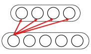
(a) input-neuron

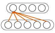
(b) output-neuron

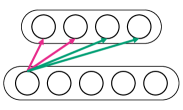
(c) partially group

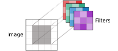
(d) filter-wise group

Figure 1: Possible examples of grouping for fully-connected layers and convolutional layers.

In the context of stochastic optimization, [2] proposed a full-matrix variant of AdaGrad. This version employs a preconditioner which exploits first-order information only, via the sum of outer products of past gradients:

$$g_{t}=\nabla f(x_{t}),\quad G_{t}=G_{t-1}+g_{t}g_{t}^{T},\quad x_{t+1}=x_{t}-\alpha_{t}(G_{t}^{1/2}+\delta I)^{-1}g_{t}$$ (1)

where $g_{t}$ is a stochastic gradient at time $t$, $\alpha_{t}$ is a step-size, and $\delta$ is a small constant for numerical stability. [2] presented theoretical regret bounds for (1) in the convex setting. However, this approach is quite expensive due to $G_{t}^{1/2}$ term, so they proposed to only use the diagonal entries of $G_{t}.$ Popular adaptive Sgd methods for training deep models such as RMSprop/Adam are based on such diagonal adaptation. Their general form and designs of the second-order momentum are given in the appendix.

[2] also discussed the case where full-matrix adaptation can converge faster than its popular diagonal counterpart. Motivated by this, we first check through a toy MLP experiment whether preconditioning with exact GOP (1) can be more effective even in the deep learning context. Our experiment shows that one can achieve faster convergence and better objective values by considering the interaction between gradient coordinates (1). Details are provided in appendix due to space constraint. The caveat here is that using full GOP adaptation in real deep learning optimization problems is computationally intractable due to the square root operator in (1). Nevertheless, is the best choice to simply use diagonal approximation given the available computation budget? What if we can afford to pay a little bit more for our computations?

Main Algorithm: Adaptive SGD with Block Diagonal Adaptation.

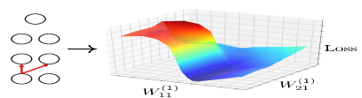
(a) From the same layer

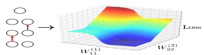
(b) From different layers

(c) RMSprop-Diag

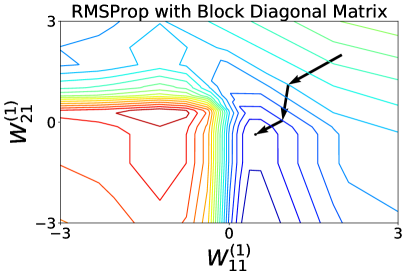
(d) RMSprop-Group

Figure 2: Top: Loss landscape for different grouping methods; Bottom: optimization trajectories on the loss landscape (a).

Algorithm 1 Adaptive Gradient Methods with Block Diagonal Matrix Adaptation

Input: Stepsize $\alpha_{t}$, initial point $x_{1}\in\mathbb{R}^{d}$, $\beta_{1}\in[0,1)$. The function $H_{t}$ designs $\widehat{V}_{t}$ with $r$ blocks.

Initialize: $m_{0}=0$, $\widehat{V}_{0}=0$. Assume $\beta_{1}\geq\beta_{1,t}$.

for $t=1,2,\ldots,T$ do

    Draw a minibatch sample $\xi_{t}$ from $\mathbb{P}$

    $i\text{ (offset)}\leftarrow 0,\quad G_{t}\leftarrow 0$

    $g_{t}$ $\leftarrow$ $\nabla f(x_{t}),~{}~{}m_{t}\leftarrow\beta_{1,t}m_{t-1}+(1-\beta_{1,t})g_{t}$

    for each group index $j=1,2,\ldots,r$ do

        $g_{t}^{(j)}$ $\leftarrow$ $g_{t}[i:i+n_{j}]$

        $G_{t}[i:i+n_{j},i:i+n_{j}]$ $\leftarrow$ $g_{t}^{(j)}\big{(}g_{t}^{(j)}\big{)}^{T}$

        $i$ $\leftarrow$ $i+n_{j}$

    end for

    $\widehat{V}_{t}$ $\leftarrow$ $H_{t}(G_{1},\cdots,G_{t})$

    $x_{t+1}$ $\leftarrow$ $x_{t}-\alpha_{t}(\widehat{V}_{t}^{1/2}+\delta I)^{-1}m_{t}$

end for

We address the above question and provide a family of adaptive Sgd bridging exact GOP adaptation and its diagonal approximation, via coordinate partitioning. Given a coordinate partition, we simply ignore the interactions of coordinates between different groups. For instance, given a gradient $g$ in a 6-dimensional space, one example of constructing block diagonal matrices via coordinate partitioning is $g=(\underbrace{g_{1},g_{2}}_{\mathcal{G}_{1}},\underbrace{g_{3},g_{4},g_{5}}_{\mathcal{G}_{2}},\underbrace{g_{6}}_{\mathcal{G}_{3}})\rightarrow[g_{{}_{\mathcal{G}_{1}}}g_{{}_{\mathcal{G}_{1}}}^{T}\mid 0\mid 0~{}\bm{;}~{}0\mid g_{{}_{\mathcal{G}_{2}}}g_{{}_{\mathcal{G}_{2}}}^{T}\mid 0~{}\bm{;}~{}0\mid 0\mid g_{{}_{\mathcal{G}_{3}}}g_{{}_{\mathcal{G}_{3}}}^{T}]$ where $\mathcal{G}_{i}$ represents each group and $g_{{}_{\mathcal{G}_{i}}}$ denotes the collection of entries corresponding to group $\mathcal{G}_{i}$. Both exact GOP and diagonal approximation are special cases of our family. Exploring the use of block-diagonal matrices was suggested as future work in [2], and our work therefore provides an in-depth study of this proposal. Our main algorithm, Algorithm 1, formalizes our approach for a total $r$ groups where each group $\mathcal{G}_{i}$ has a size of $n_{i}$ for $i\in[r]$. The Algorithm 1 can handle arbitrary coordinate grouping with appropriate reordering of entries, and groups of unequal sizes.

Effect of grouping on optimization. Figure 1 shows some grouping examples in the context of deep learning models: grouping the weights with the same color in a neural network can approximate the exact GOP matrix with a block diagonal matrix of several small full matrices. To see which grouping could be more effective in terms of optimization, we revisit our MLP toy example. Figure 2-(a,b) show the loss landscape for different grouping strategies (weights other than shown are fixed as true model values). It can be seen that the loss landscape when grouping weights in the same layer has a much more dynamic curvature than when grouping weights in different layers. In this context, we expect that a preconditioner based on block-diagonal matrices is effective in terms of optimization and illustrate this empirically by comparing the grouping version for the loss landscape with dynamic curvature (Figure 2-(a)), and its diagonal counterpart. To figure out the effect of the block-diagonal based matrix preconditioner only, we compare both approaches using RMSprop which does not consider the first-order momentum. Figure 2-(c,d) illustrate the optimization trajectories. The block diagonal version of RMSprop converges to a stationary point in fewer steps than the diagonal approximation and shows a more stable trajectory.

Computations and memory considerations compared to full matrix adaptation as well as its modified version GGT are discussed in the appendix.

3 Convergence Analysis

In this section, we provide a theoretical analysis of the convergence of Algorithm 1. We consider the following non-convex optimization problem, $\min f(x)\coloneqq\mathbb{E}_{\xi\sim\mathbb{P}}\big{[}f(x;\xi)\big{]}$ where $x$ is an optimization variable and $\xi$ is a random variable representing randomly selected data sample from $\mathcal{D}$. While $f$ is assumed to be continuously differentiable with Lipschitz continuous gradient, it can be non-convex. In non-convex optimization, we study convergence to “stationarity” and hence derive upper bounds for $\|\nabla f(x)\|^{2}$ as in [14, 15]. We assume $\widehat{V}_{t}$ in Algorithm 1 has $r$ blocks, $\{\widehat{B}_{t,[j]}\}_{j=1}^{r}$. Our analysis covers two settings: when the minibatch size $M$ is fixed and when $M$ is increasing during training.

Convergence for Fixed Minibatch size.

First, we provide sufficient conditions for our algorithms to converge and difference with diagonal counterpart, for fixed minibatch size. We make the following assumptions.

Assumption 1.

(a) $f$ is differentiable and has $L$-Lipschitz gradients. $f$ is also lower bounded. (b) At time $t$, the algorithm can access a bounded noisy gradient. We assume the true gradient and noisy gradient are both bounded, i.e. $\|\nabla f(x_{t})\|_{\infty},\|g_{t}\|_{\infty}\leq G_{\infty}$ for all $t$. (c) The noisy gradient $g_{t}$ is unbiased and the noise is independent, i.e. $g_{t}=\nabla f(x_{t})+\zeta_{t}$ where $\mathbb{E}[\zeta_{t}]=0$ and $\zeta_{i}$ is independent of $\zeta_{j}$ for $i\neq j$. (d) $\beta_{1}\geq\beta_{1,t},\beta_{1,t}\in[0,1)$ is non-increasing. (e) For some constant $D_{\infty}>0$, $\|\alpha_{t}\widehat{V}_{t}^{-1/2}m_{t}\|\leq D_{\infty}$.

Here, we assume $\delta I$ is absorbed in $\widehat{V}_{t}$. Assumption 1 are also needed for the diagonal case [11]. Condition (a) is a key assumption in general non-convex optimization analysis, and (b)-(d) are standard ones in this line of work. The last condition (e) states that the final step vector $\alpha_{t}\widehat{V}_{t}^{-1/2}m_{t}$ should be finite, which is a mild condition. We are now ready to state our first theorem.

Theorem 1.

For the Algorithm 1, define the quantity $Q_{t}\coloneqq|\!|\!|\alpha_{t}\widehat{V}_{t}^{-1/2}-\alpha_{t-1}\widehat{V}_{t-1}^{-1/2}|\!|\!|_{2}=\max_{j\in[r]}\{|\!|\!|\alpha_{t}\widehat{B}_{t,[j]}^{-1/2}-\alpha_{t-1}\widehat{B}_{t-1,[j]}^{-1/2}|\!|\!|_{2}\}$ which measures the maximum difference in effective spectrums over all blocks $\widehat{B}_{t,[j]}$. Under the Assumption 1, the Algorithm 1 yields

$$\mathbb{E}\Bigg{[}\sum\limits_{t=1}^{T}\alpha_{t}\Big{\langle}\nabla f(x_{t}),\widehat{V}_{t}^{-\frac{1}{2}}\nabla f(x_{t})\Big{\rangle}\Bigg{]}\leq\mathbb{E}\Bigg{[}C_{1}\sum\limits_{t=1}^{T}\underbrace{\|\alpha_{t}\widehat{V}_{t}^{-\frac{1}{2}}g_{t}\|^{2}}_{\text{Term A}}+~{}C_{2}\sum\limits_{t=2}^{T}\underbrace{Q_{t}}_{\text{Term B}}+~{}C_{3}\sum\limits_{t=2}^{T-1}Q_{t}^{2}\Bigg{]}+C_{4}$$ (2)

where $C_{1},C_{2},$ and $C_{3}$ are constants independent of $d$ and $T$, $C_{4}$ is a constant independent of $T$. The expectation is taken with respect to all the randomness corresponding to $\{g_{t}\}_{t=1}^{T}$.  
Further, we let $\gamma_{t}\coloneqq\min_{\{g_{t}\}_{t=1}^{T}}\lambda_{min}(\alpha_{t}\widehat{V}_{t}^{-1/2})$ denote the possible minimum effective spectrum over all past gradients. Then, we have $\min_{t\in[T]}\mathbb{E}\big{[}\|\nabla f(x_{t})\|^{2}\big{]}=O\big{(}\frac{s_{1}(T)}{s_{2}(T)}\big{)}$ where $s_{1}(T)$ is defined as the upper bound in (2), namely, $\mathcal{O}\big{(}s_{1}(T)\big{)}$, and $\sum_{t=1}^{T}\gamma_{t}=\Omega\big{(}s_{2}(T)\big{)}$.

Remarks. Our first theorem provides sufficient conditions, $s_{1}(T)=o\big{(}s_{2}(T)\big{)}$, for convergence as in the diagonal case [11]. The convergence of block-diagonal and diagonal versions depend on the dynamics of Term A and Term B as noted in [11] and in our theorem. The Term A for block diagonal version is $\|\alpha_{t}\widehat{V}_{t}^{-1/2}g_{t}\|^{2}$ and for diagonal version is $\|\alpha_{t}g_{t}/\sqrt{\widehat{v}_{t}}\|^{2}$. The Term B for block diagonal version is $|\!|\!|\alpha_{t}\widehat{V}_{t}^{-1/2}-\alpha_{t-1}\widehat{V}_{t-1}^{-1/2}|\!|\!|_{2}$ and for diagonal version is $\|\alpha_{t}/\sqrt{\widehat{v}_{t}}-\alpha_{t-1}/\sqrt{\widehat{v}_{t-1}}\|_{1}$. We can see that the main difference is in Term B.

If we assume grouping size of 1 in our Algorithm 1, i.e. $r=d$, $\widehat{V}_{t}$ becomes a diagonal matrix. In this case, Term B for the block diagonal version represents the maximum difference of effective learning rate while Term B for the diagonal version means the sum of differences of effective learning rate over all coordinates. Therefore, our bound improves upon prior results even for the diagonal case. The difference comes from the proofs. The proofs of prior analysis for diagonal case depends on the coordinate-wise effective stepsize, but this term is absent in our case. Our proofs rely on the matrix norm which allows smaller bound. To investigate the difference for general group size, we perform an empirical evaluation through MNIST classification task using 784-100-10 MLP with fixed minibatch size 128, and group size of 10. Figure 3 illustrates the dynamics of Term A and Term B, supporting our observations by showing a big difference for Term B. As we observe significant improvement in Term B, we expect that block diagonal matrix approximation can alleviate the oscillatory behavior of diagonal version, and we corroborate this by empirical studies on more architectures in Section 5.

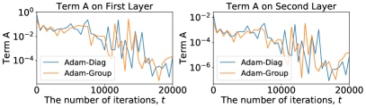
(a) Term A

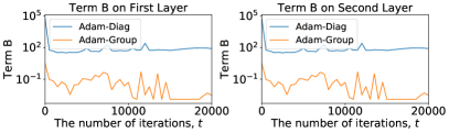
(b) Term B

Figure 3: Dynamics of Term A and Term B for block diagonal version with group size of $10$ and diagonal version. Both approaches have similar scale of Term A, but there are big differences in Term B for both layers. For fair comparisons, we set $\delta=\epsilon=10^{-4}$.

We instantiate our theorem to AdaGrad/AdaFom[16, 17] satisfying the sufficient conditions.

Corollary 1.

(AdaGrad/AdaFom) If we set $\alpha_{t}=1/\sqrt{t}$ and $\beta_{1,t}\leq\beta_{1}\in[0,1)$ and $\beta_{1,t}$ is non-increasing ($\beta_{1}=0$ for AdaGrad), AdaGrad/AdaFom with block diagonal matrix adaptations achieve $\min_{t\in[T]}\mathbb{E}\big{[}\|\nabla f(x_{t})\|^{2}\big{]}=\mathcal{O}(\log T/\sqrt{T})$.

This is the same convergence rate as diagonal versions [16, 17]. As discussed in remarks, we expect that it is possible to remove the $\log T$ term since block diagonal matrix adaptation can have smaller bound, but this is an open question.

Convergence of Block-diagonal RMSprop and Adam with Increasing Minibatch Size.

Moving on to the case of increasing minibatch size, we show that algorithms based on EMA such as RMSprop/Adam with block diagonal matrix adaptation converge to a stationary point. This is the case of our Algorithm 1 with $H_{t}=\beta_{2}\widehat{V}_{t-1}+(1-\beta_{2})g_{t}g_{t}^{T}$. We assume bounded variance of stochastic gradients, $\mathbb{E}\big{[}\|\nabla f(x;\xi)-\nabla f(x)\|^{2}\big{]}\leq\sigma^{2}$, a standard assumption in analyses of stochastic gradient methods [14, 15]. We are ready to state our second theorem.

Theorem 2.

(RMSprop/Adam) For the Algorithm 1, define the quantity $\kappa_{t}\coloneqq\kappa(\beta_{2}^{1/2}\widehat{V}_{t}^{1/2}+\delta I)$. Under the Assumption 1 (without (e)) and bounded variance of gradients, we suppose that $\kappa_{t}$ is bounded above by $\kappa_{\text{max}}$ and $\alpha_{t}=\alpha$  for all $t$. Furthermore, we assume that all blocks $\{\widehat{B}_{t,[j]}\}_{j=1}^{r}$ are full-rank when $t\geq t_{0}$ for some $t_{0}\in\mathbb{N}$ and $\beta_{1,t}=\beta_{1}\lambda^{t-1}$ for some $\lambda\in(0,1)$. If the parameters $\alpha$, $\beta_{2}$, and $\delta$ are chosen such that $1-\beta_{2}\leq\frac{\delta^{2}}{9G_{\infty}^{2}\kappa_{\text{max}}^{2}},$ and $\alpha\leq\frac{2\delta}{3L\kappa_{\text{max}}}$. Then, the iterates $x_{t}$ generated by the Algorithm 1 satisfies

$$\min\limits_{t\in[T]}\mathbb{E}\big{[}\|\nabla f(x_{t})\|^{2}\big{]} \leq\frac{3(\sqrt{\beta_{2}}G_{\infty}+\delta)}{1-\beta_{1}}\Bigg{[}\frac{f(x_{t_{0}})-f(x^{*})}{\alpha T}+\frac{\sigma^{2}}{M}\Big{(}\frac{G_{\infty}\sqrt{1-\beta_{2}}}{\delta^{2}}+\frac{\alpha L}{2\delta^{2}}\Big{)}+\frac{C}{T}\Bigg{]}$$

which is $\mathcal{O}(1/T+\sigma^{2}/M)$, where $C$ is a constant independent of $T$ and $x^{*}$ is an optimal solution. Additionally, we can obtain the bound for RMSprop if we set $\beta_{1}=0$.

Remarks. If we consider exact GOP, i.e. $r=1$, $\widehat{V}_{t}$ is an exact full GOP and the condition that $\widehat{V}_{t}$ becomes full-rank within finite time $t_{0}$ may not be satisfied. For instance, consider the least-square problem with $y=X\beta+\epsilon$ where $(X,y)$ is a given data, $\theta$ is a parameter we should optimize, and $\epsilon$ is a noise. For this case, the GOP matrix contains $X^{T}XX^{T}X$, so it is always rank-deficient in the high-dimensional setting. In contrast, we emphasize that Theorem 2 can be applied to block diagonal matrix adaptations, because we only require the full-rankness of each small sub-matrix $\widehat{B}_{t,[j]}$.

The condition on $\kappa_{\text{max}}$ states that $\kappa_{\text{max}}$ should be bounded above by some constant. Therefore, the condition number of $(\beta_{2}^{1/2}\widehat{V}_{t}^{1/2}+\delta I)$ at time $t$ should not be “too” large (i.e. not too ill-conditioned), so we choose $\delta$ not too small. On the other hand, we cannot unconditionally increase $\delta$ since the first term $\frac{3(\sqrt{\beta_{2}}G_{\infty}+\delta)}{(1-\beta_{1})}\times\frac{f(x_{t_{0}})-f(x_{T})}{\alpha T}$ tends to diverge as $\delta$ increases. Balancing these two, we use $\delta=10^{-4}$ for our experiments, instead of $\delta=10^{-8}$ which is recommended for diagonal case.

Lastly, we need $M=\mathcal{O}(T)$ to guarantee convergence. However, this condition is not stringent. As a concrete example, consider a problem with sample size $N$ and minibatch size $M$ with maximum 200 epochs. Since the minibatch size is $M$, $T$ should be $\mathcal{O}(\frac{200N}{M})$ resulting in $M=\mathcal{O}(10\sqrt{2N})=\mathcal{O}(\sqrt{N})$, which is practical in real cases.

4 Interpolation with SGD via Spectrum-Clipping

It has been shown in [8] that adaptive methods are better than vanilla Sgd in the early stage but get worse as the learning process matures. To address this, [18] suggests training networks with Adam at the beginning and switching to Sgd later. [10] proposes methods AdaBound/AMSBound which clip the effective learning rate $\alpha_{t}/(\sqrt{\widehat{v}_{t}}+\epsilon)$ of Adam by decreasing sequence of intervals $I_{t}=[\eta_{l}(t),\eta_{u}(t)]$ every iteration which converges to some point, thereby resembling Sgd in the end. However, this type of extension is not obvious in our framework due to the absence of effective learning rate in our case. Instead, we observe that the spectral property is important in our convergence analysis (In Theorem 1: convergence heavily depends on Term B, maximum changes in effective spectrum, $|\!|\!|\alpha_{t}\widehat{V}_{t}^{-1/2}-\alpha_{t-1}\widehat{V}_{t-1}^{-1/2}|\!|\!|_{2}$. In Theorem 2, we need conditions on $\kappa(\beta_{2}^{1/2}\widehat{V}_{t}^{1/2}+\delta I)$). Motivated on them, we propose a spectrum-clipping scheme which clips the spectrum of $\alpha_{t}(\widehat{V}_{t}^{1/2}+\delta I)^{-1}$ by decreasing sequence of intervals. For spectrum-clipping, we use the following modified update rule in Algorithm 1 after constructing $\widehat{V}_{t}$: (i) $\widehat{U}_{t},\widehat{\Sigma}_{t}^{1/2},\_\leftarrow\mathrm{SVD}(\widehat{V}_{t}^{1/2})$, (ii) $\widetilde{\Sigma}_{t}^{-1/2}\leftarrow\mathrm{Clip}(\lambda(\alpha_{t}(\widehat{\Sigma}_{t}^{1/2}+\delta I)^{-1}),\lambda_{l}(t),\lambda_{u}(t)\big{)}$, and (iii) $x_{t+1}\leftarrow x_{t}-\widehat{U}_{t}^{T}\widetilde{\Sigma}_{t}^{-1/2}\widehat{U}_{t}m_{t}$. We schedule the sizes of clipping intervals converging to a single point uniformly over all coordinates so that $\alpha_{t}(\widehat{V}_{t}^{1/2}+\delta I)^{-1}$ can be easily computed in the form of constant times identity matrix and effectively behaves like vanilla Sgd. In all our experiments, we use $\lambda_{l}(t)=(1-\frac{1}{\gamma t+1})\alpha^{*}$ and $\lambda_{u}(t)=(1+\frac{1}{\gamma t})\alpha^{*}$ where $\gamma$ reflects the clipping speed and $\alpha^{*}$ represents the final learning rate of vanilla Sgd, as in [10]. We specify how to choose $\gamma$ and $\alpha^{*}$ in Section 5.

5 Experiments

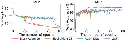
(a) MLP for Adam

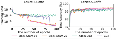
(b) LeNet-5-Caffe for Adam

Figure 4: Training loss and test accuracy for MLP/LeNet-5-Caffe on MNIST dataset.

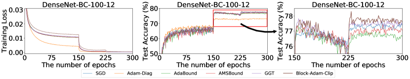
(a) Training loss and test accuracy for DenseNet-BC-100-12 on CIFAR-100.

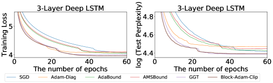
(b) Training loss and test perplexity for 3-layer deep LSTM on PTB

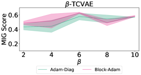
(c) MIG Score on $\beta$-TCVAE

Figure 5: Results on (a) CIFAR classification, (b) language models, (c) generative models.

We consider two sets of experiments. The first shows the differences between block-diagonal and diagonal versions. The second investigates whether block diagonal matrix adaptation can achieve state-of-the-art performance on benchmark architecture/dataset for various important deep learning problems. For the first set, we do not consider the spectrum-clipping of Section 4, to clearly assess the effect of coordinate partitioning. In our Algorithm 1, coordinate grouping can be done in a number of ways. Given our insight that grouping weights in the same layer could be more effective, we consider Figure 1-(c) with grouping 10 or 25 weight parameters connected to input-neuron for fully-connected layer, and we consider filter-wise grouping for convolutional layers as in Figure 1-(d). We add a suffix Block for our optimizer such as Block-Adam, representing the Adam with block diagonal matrix adaptations. Details on hyperparameter choices for each experiment are provided in the appendix.

Investigating Grouping Effect. We investigate the effect of coordinate partitioning on MNIST classification and generative models.

MNIST Classification. We consider a fully connected model, LeNet-300-100 [19], and a simple convolutional network, LeNet-5-Caffe. We use 128 mini-batch size and train networks with maximum 100 epochs. To see the effect of coordinate grouping, we compare RMSProp/Adam with block diagonal matrix version and diagonal counterpart. Figure 4 illustrates the results for Adam, and the results for RMSprop are in the appendix. The learning curve looks similar in the early stage of training, but our methods converge without oscillatory behavior in the latter part of training, which corroborates our observations on Theorem 1. The generalization of block-diagonal approaches also becomes more stable than diagonal variant and GGT, and overall superior across epochs.

Generative Models. We conduct experiments on very recent variant of VAE called $\beta$-TCVAE [20]. The goal of this model is to make the encoder $q(z|x)$ give disentangled representation $z$ of input images $x$ by additionally forcing $q(z)=\int q(z|x)p(x)dx$ to be factorized, which can be achieved by giving heavier penalty on total correlation. We evaluate our optimizer with the Mutual Information Gap (MIG) score they proposed, to measure disentanglement of the latent code. Following implementation in [20], we use convolutional encoder-decoder for $\beta$-TCVAE on 3D faces dataset [21]. Figure 5-(c) illustrates the results over 5 random simulations with $95\%$ confidence region. The block diagonal version outperforms diagonal version except at $\beta=8$, and we can achieve the best performance at $\beta=6$, which is a recommended value for $\beta$-TCVAE [20].

Improving Performance with Spectrum-Clipping. We demonstrate the superiority of our algorithms using more complex benchmark architecture/dataset for two popular tasks in deep learning: image classification and language modeling. For both tasks, vanilla Sgd with proper learning rate scheduling has enjoyed state-of-the-art performance. Therefore, we compare algorithms using our spectrum-clipping methods that can exploit higher generalization ability of vanilla Sgd.

Table 1: Test error (%) for CIFAR dataset.

	SGD	Adam	Ada- Bound	Ams- Bound	GGT	Block- Adam
CIFAR-10	4.51	6.07	4.78	4.77	6.33	4.34
CIFAR-100	22.27	26.51	22.5	22.52	22.17	21.7

CIFAR Classification. We conduct experiments using DenseNet architecture [22]. Figure 5-(a) illustrates our results on CIFAR-100 datasets, and the figure for CIFAR-10 is in appendix. In both cases, the training speed of our algorithm at the early stage is similar or slightly slower, but we can arrive at the state-of-the-art generalization performance in the end among all comparison algorithms. Specifically, we can achieve great improvement in generalization about $0.5\%$ for CIFAR-100 dataset as in Table 1. Note that, our spectrum-clipping method consistently achieves higher performance.

Language Models. We use recurrent networks [23], base architectures still frequently used today for language modeling. While [23] uses only two layers maximum, we add one more layer to consider more complex and deeper networks. To consider similar model capacity as [23], we use 500 hidden units on each layer. Based on this architecture, we build a word-level language model using 3-layer LSTM [24] on Penn TreeBank (PTB) dataset [25]. Figure 5-(b) shows the experimental results: the optimizer with spectrum-clipping of Adam outperforms all the other algorithms w.r.t. learning curve. It achieves similar perplexity as GGT and outperforms the other methods.

6 Concluding Remarks

We proposed a general adaptive gradient framework that approximates exact GOP with block diagonal matrices via coordinate grouping, and showed that it can be a practical and powerful solution that can effectively utilize structural characteristics of deep learning architectures. We analyzed convergence for our approach, showed that they can lead to a smaller upper bound than its popular diagonal counterpart, and confirmed our findings empirically. We also proposed a spectrum-clipping algorithm which achieved state-of-the-art generalization performance on popular deep learning tasks. As future work, we plan to explore additional strategies for setting the clipping parameters in our approach to strike the best balance between training speed and generalization ability, and to develop novel computationally efficient methods that generalize well.

Supplementary Materials

Appendix A Toy MLP example: Full GOP adaptation vs. Diagonal approximation

We consider a structured MLP (two nodes in two hidden layers followed by single output). For hidden units, we use ReLU activation [26] and the sigmoid unit for the binary output. We generate $n=10$ i.i.d. observations: $x_{i}\sim\mathcal{N}(0,I_{2})$ and $y_{i}$ from this two layered MLP given $x_{i}$. The results of our toy experiment are depicted in Figure 6.

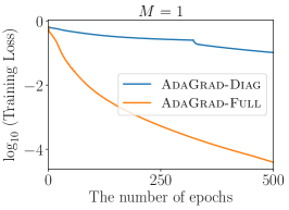
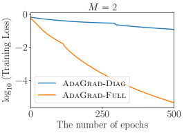
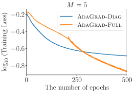
Figure 6: Comparison of AdaGrad diagonal version and full matrix version varying the minibatch size $M$.

Appendix B Computations and memory considerations

Compared with full matrix adaptation, working with a block diagonal matrix is computationally more efficient as it allows for decoupling computations with respect to each small full sub-matrix. In Algorithm 1, the procedures for constructing the block diagonal matrix and for updating parameters for each block by computing the “inverse” square root of each sub-matrix can be done in a parallel manner. As the group size increases, the block diagonal matrix becomes closer to the full matrix, resulting in greater computational cost. Therefore, we consider small group size for our numerical experiments. Although the wall clock time of Block-Adam for experiments on CIFAR dataset is about two times more than the diagonal counterpart, our results show great improvement in generalization. In terms of memory, our method is more efficient than GGT [13] (the modified version of full-matrix Adagrad). For example, consider models with a total of $d$ parameters. For Algorithm 1, assume that $\widehat{V}_{t}$ is a block diagonal matrix with $r$ sub-matrices, and each block has size $m\times m$ (so, $rm=d$). Also, assume that the truncated window size for GGT is $w$. GGT needs a memory size of $\mathcal{O}(wd)$, and our algorithm requires $\mathcal{O}(rm^{2})=\mathcal{O}(md)$. We consider small group size $m=10$ or $25$ for our experiments while the recommended window size of GGT is 200 [13]. Therefore, our algorithm is more memory-efficient and the benefit is more pronounced as the number of model parameters $d$ is large, which is the case in popular deep learning models/architectures.

Appendix C Hyperparameters and Additional Experimental Results

We use the recommended step size or tune it in the range $[10^{-4},10^{2}]$ for all comparison algorithms. For Adam based algorithms, we use default decay parameters $(\beta_{1},\beta_{2})=(0.9,0.999)$. For a diagonal version of Adam variant algorithm, we choose numerical stability parameter $\epsilon=10^{-4}$ (to match our choice of $\delta=10^{-4}$) for fair comparison since the larger value of $\epsilon$ can improve the generalization performance as discussed in [12]. For $\gamma$ and $\alpha^{*}$ in clipping bound functions, we consider $\gamma\in\{10^{-3},10^{-4}\}$ and choose $\alpha^{*}\in\{\alpha_{\textrm{SGD}},10\alpha_{\textrm{SGD}}\}$ where $\alpha_{\textrm{SGD}}$ is the best-performing initial learning rate for vanilla Sgd (These hyperparameter candidates are based on the empirical studies in [10]). As in [10], our results are also not sensitive to choice of $\gamma$ and $\alpha^{*}$. With these hyperparameters, we consider maximum 300 epochs training time, and mini-batch size or learning rate scheduling are introduced in each experiment description. Our Algorithm 2 requires $\mathrm{SVD}$ procedures to compute the square root of a block diagonal matrix. We apply $\mathrm{SVD}$ efficiently to all small sub-matrices simultaneously through batch mode of $\mathrm{SVD}$.

Generative Models.

For experiments on generative models $\beta$-TCVAE, we use the author’s implementation only replacing the Adam optimizer with our Block-Adam. We use convolutional networks for encoder-decoder and mini-batch size 2048.

CIFAR classification.

According to experiment settings in [22], we use mini-batch size 64 and consider maximum 300 epochs. Also, we use a step-decay learning rate scheduling in which the learning rate is divided by $10$ at $50\%$ and $75\%$ of the total number of training epochs. With this setting, vanilla Sgd with a momentum factor 0.9 performs best with initial learning rate $\alpha^{*}=0.1$, so we use this value for our bound functions of spectrum-clipping, $\lambda_{l}(t)$ and $\lambda_{u}(t)$.

Language Models.

In this experiment, we use a dev-decay learning rate scheduling [8] where we reduce learning rate by a constant factor if the model does not attain a new best validation performance at each epoch as in [23]. Under this setting, vanilla Sgd performs best when the initial learning rate $\alpha^{*}=5$.

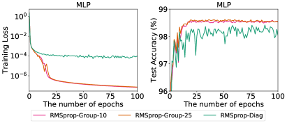
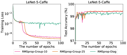
Figure 7: Training curve and test accuracy for MLP/LeNet-5-Caffe with RMSprop.

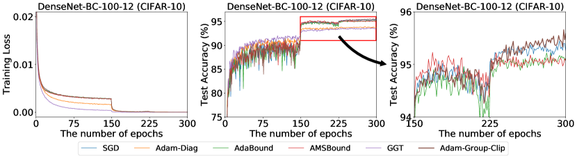
Figure 8: Training curve and test accuracy for DenseNet-BC-100-12 on CIFAR-10 dataset.

Appendix D General Frameworks

Algorithm 2 Adaptive Gradient Methods with Block Diagonal Matrix Adaptations via Grouping

Input: Stepsize $\alpha_{t}$, initial point $x_{1}\in\mathbb{R}^{d}$, $\beta_{1}\in[0,1)$, and the function $H_{t}$ which designs $\widehat{V}_{t}$.

Initialize: $m_{0}=0$, $\widehat{V}_{0}=0$, and $t=0$.

Assumption: We have $r$ blocks with each size $n_{i}\times n_{i}$ and $n_{1}+\cdots+n_{r}=d$, and $\beta_{1,t}\geq\beta_{1,t+1}$

for $t=1,2,\ldots,T$ do

    Draw a minibatch sample $\xi_{t}$ from $\mathbb{P}$

    offset $\leftarrow$ 0

    $G_{t}$ $\leftarrow$ 0

    $g_{t}$ $\leftarrow$ $\nabla f(x_{t})$

    $m_{t}$ $\leftarrow$ $\beta_{1,t}m_{t-1}+(1-\beta_{1,t})g_{t}$

    for each group index $j=1,2,\ldots,r$ do

         $g_{t}^{(j)}$ $\leftarrow$ $g_{t}[\text{offset}:{\text{offset}+n_{j}}]$

         $G_{t}[\text{offset}:{\text{offset}+n_{j}},\text{offset}:{\text{offset}+n_{j}}]$ $\leftarrow$ $g_{t}^{(j)}\big{(}g_{t}^{(j)}\big{)}^{T}$

         offset $\leftarrow$ offset + $n_{j}$

    end for

    $\widehat{V}_{t}$ $\leftarrow$ $H_{t}(G_{1},\cdots,G_{t})$

    $x_{t+1}$ $\leftarrow$ $x_{t}-\alpha_{t}(\widehat{V}_{t}^{1/2}+\delta I)^{-1}m_{t}$

end for

We provide the general frameworks of adaptive gradient methods with exact full matrix adaptations. The Algorithm 3 and 4 represent the general framework for each case. We can identify algorithms according to the functions $h_{t}$ (Table 2) and $H_{t}$ (Table 3) which determine the dynamics of $\widehat{v}_{t}$ and $\widehat{V}_{t}$ respectively. Also, the Algorithm 2 is a detail version of the Algorithm 1.

Algorithm 3 General Adaptive Gradient Methods approximating $g_{t}g_{t}^{T}$ via Diagonal Matrix

Input: Initial point $x_{1}\in\mathbb{R}^{d}$, stepsize $\{\alpha_{t}\}_{t=1}^{T}$, decay parameters $\beta_{1,t},\beta_{2}\in[0,1]$, and $\epsilon>0$.

Initialize: $m_{0}=0$, $\widehat{v}_{0}=0$.

for $t=1,2,\ldots,T$ do

    Draw a minibatch sample $\xi_{t}$ from $\mathbb{P}$

    $g_{t}$ $\leftarrow$ $\nabla f(x_{t};\xi_{t})$

    $G_{t}$ $\leftarrow$ $\mathrm{diag}(g_{t}g_{t}^{T})$

    $m_{t}$ $\leftarrow$ $\beta_{1,t}m_{t-1}+(1-\beta_{1,t})g_{t}$

    $\widehat{v}_{t}$ $\leftarrow$ $h_{t}(G_{1},G_{2},\ldots,G_{t})$

    $x_{t+1}$ $\leftarrow$ $x_{t}-\alpha_{t}m_{t}/(\sqrt{\widehat{v}_{t}}+\epsilon)$

end for

Output: $\widehat{x}$.

Algorithm 4 General Adaptive Gradient Methods with the exact $g_{t}g_{t}^{T}$ (Full Matrix)

Input: Initial point $x_{1}\in\mathbb{R}^{d}$, stepsize $\{\alpha_{t}\}_{t=1}^{T}$, decay parameters $\beta_{1,t},\beta_{2}\in[0,1]$, and $\delta>0$.

Initialize: $m_{0}=0$, $\widehat{V}_{0}=0$.

for $t=1,2,\ldots,T$ do

    Draw a minibatch sample $\xi_{t}$ from $\mathbb{P}$

    $g_{t}$ $\leftarrow$ $\nabla f(x_{t};\xi_{t})$

    $G_{t}$ $\leftarrow$ $g_{t}g_{t}^{T}$

    $m_{t}$ $\leftarrow$ $\beta_{1,t}m_{t-1}+(1-\beta_{1,t})g_{t}$

    $\widehat{V}_{t}$ $\leftarrow$ $H_{t}(G_{1},G_{2},\ldots,G_{t})$

    $x_{t+1}$ $\leftarrow$ $x_{t}-\alpha_{t}(\widehat{V}_{t}^{1/2}+\delta I)^{-1}m_{t}$

end for

Output: $\widehat{x}$.

Table 2: Variants of diagonal matrix adaptations

	$\beta_{1,t}=0$	$\beta_{1,t}=\beta_{1}$
$1$	Sgd	-
$(1/t)\sum_{t=1}^{T}g_{t}^{2}$	AdaGrad	AdaFom
$\beta_{2}\widehat{v}_{t-1}+(1-\beta_{2})g_{t}^{2}$	RMSProp	Adam
$v_{t}=\beta_{2}v_{t-1}+(1-\beta_{2})g_{t}^{2}$,
$\widehat{v}_{t}=\max\{\widehat{v}_{t-1},v_{t}\}$	-	AMSGrad

Table 3: Variants of full matrix adaptations

	$\beta_{1,t}=0$	$\beta_{1,t}=\beta_{1}$
$\widehat{V}_{t}=I$	Sgd	-
$\widehat{V}_{t}=\frac{1}{T}\sum_{t=1}^{T}g_{t}g_{t}^{T}$	AdaGrad	AdaFom
$\widehat{V}_{t}=\beta_{2}\widehat{V}_{t-1}+(1-\beta_{2})g_{t}g_{t}^{T}$	RMSProp	Adam
$V_{t}=U_{t}\Sigma_{t}U_{t}^{T}$,
$\widehat{V}_{t}=U_{t}\max\{\widehat{\Sigma}_{t-1},\Sigma_{t}\}U_{t}^{T}$	-	AMSGrad

Appendix E Proofs of Main Theorems

We study the following minimization problem,

$$\min f(x)\coloneqq\mathbb{E}_{\xi}[f(x;\xi)]$$

under the assumption 1. The parameter $x$ is an optimization variable, and $\xi$ is a random variable representing randomly selected data sample from $\mathcal{D}$. We study the convergence analysis of the algorithm 2. For analysis in stochastic convex optimization, one can refer to [2]. For analysis in non-convex optimization with full matrix adaptations, we follow the arguments in the paper [11]. As we will show, the convergence of the adaptive full matrix adaptations depends on the changes of effective spectrum while the diagonal counterpart depends on the changes of effective stepsize. We assume that $\delta I$ is absorbed into $\widehat{V}^{-1/2}$ for convenience of notations. Note that, our proof can be applied to exact full matrix adaptations, algorithm 4.

E.1 Technical Lemmas for Theorem 1

Lemma 1.

Consider the sequence

$$z_{t}=x_{t}+\frac{\beta_{1,t}}{1-\beta_{1,t}}(x_{t}-x_{t-1})$$

Then, the following holds true

$$z_{t+1}-z_{t}=-\Bigg{(}\frac{\beta_{1,t+1}}{1-\beta_{1,t+1}}-\frac{\beta_{1,t}}{1-\beta_{1,t}}\Bigg{)}\alpha_{t}\widehat{V}_{t}^{-1/2}m_{t}-\frac{\beta_{1,t}}{1-\beta_{1,t}}\Bigg{(}\alpha_{t}\widehat{V}_{t}^{-1/2}-\alpha_{t-1}\widehat{V}_{t-1}^{-1/2}\Bigg{)}m_{t-1}-\alpha_{t}\widehat{V}_{t}^{-1/2}g_{t}$$

Proof.

By our update rule, we can derive

$$x_{t+1}-x_{t}=~{} -\alpha_{t}\widehat{V}_{t}^{-1/2}m_{t}$$

$$\overset{(i)}{=}~{} -\alpha_{t}\widehat{V}_{t}^{-1/2}(\beta_{1,t}m_{t-1}+(1-\beta_{1,t})g_{t})$$

$$=~{} -\alpha_{t}\beta_{1,t}\widehat{V}_{t}^{-1/2}m_{t-1}-\alpha_{t}(1-\beta_{1,t})\widehat{V}_{t}^{-1/2}g_{t}$$

$$\overset{(ii)}{=} -\alpha_{t}\beta_{1,t}\widehat{V}_{t}^{-1/2}\Big{(}-\frac{1}{\alpha_{t-1}}\widehat{V}_{t-1}^{1/2}(x_{t}-x_{t-1})\Big{)}-\alpha_{t}(1-\beta_{1,t})\widehat{V}_{t}^{-1/2}g_{t}$$

$$=~{} \frac{\alpha_{t}}{\alpha_{t-1}}\beta_{1,t}(\widehat{V}_{t}^{-1}\widehat{V}_{t-1})^{1/2}(x_{t}-x_{t-1})-\alpha_{t}(1-\beta_{1,t})\widehat{V}_{t}^{-1/2}g_{t}$$

$$=~{} \beta_{1,t}(x_{t}-x_{t-1})+\beta_{1,t}\Bigg{(}\frac{\alpha_{t}}{\alpha_{t-1}}(\widehat{V}_{t}^{-1}\widehat{V}_{t-1})^{1/2}-I_{d}\Bigg{)}(x_{t}-x_{t-1})-\alpha_{t}(1-\beta_{1,t})\widehat{V}_{t}^{-1/2}g_{t}$$

$$\overset{(iii)}{=}~{} \beta_{1,t}(x_{t}-x_{t-1})-\beta_{1,t}\Bigg{(}\alpha_{t}\widehat{V}_{t}^{-1/2}-\alpha_{t-1}\widehat{V}_{t-1}^{-1/2}\Bigg{)}m_{t-1}-\alpha_{t}(1-\beta_{1,t})\widehat{V}_{t}^{-1/2}g_{t}$$

The reasoning follows

1. By definition of $m_{t}$.

2. Since $x_{t}=x_{t-1}-\alpha_{t-1}\widehat{V}_{t-1}^{-1/2}m_{t-1}$, we can solve as $m_{t-1}=-\frac{1}{\alpha_{t-1}}\widehat{V}_{t-1}^{1/2}(x_{t}-x_{t-1})$.

3. Similarly to (ii), we can have $\widehat{V}_{t-1}^{1/2}(x_{t}-x_{t-1})/\alpha_{t-1}=-m_{t-1}$.

Since $x_{t+1}-x_{t}=(1-\beta_{1,t})x_{t+1}+\beta_{1,t}(x_{t+1}-x_{t})-(1-\beta_{1,t})x_{t}$, we can further derive by combining the above,

$$(1-\beta_{1,t})x_{t+1}+\beta_{1,t}(x_{t+1}-x_{t})$$

$$=~{} (1-\beta_{1,t})x_{t}+\beta_{1,t}(x_{t}-x_{t-1})-\beta_{1,t}\Bigg{(}\alpha_{t}\widehat{V}_{t}^{-1/2}-\alpha_{t-1}\widehat{V}_{t-1}^{-1/2}\Bigg{)}m_{t-1}-\alpha_{t}(1-\beta_{1,t})\widehat{V}_{t}^{-1/2}g_{t}$$

By dividing both sides by $1-\beta_{1,t}$,

$$x_{t+1}+\frac{\beta_{1,t}}{1-\beta_{1,t}}(x_{t+1}-x_{t})$$

$$=~{} x_{t}+\frac{\beta_{1,t}}{1-\beta_{1,t}}(x_{t}-x_{t-1})-\frac{\beta_{1,t}}{1-\beta_{1,t}}\Bigg{(}\alpha_{t}\widehat{V}_{t}^{-1/2}-\alpha_{t-1}\widehat{V}_{t-1}^{-1/2}\Bigg{)}m_{t-1}-\alpha_{t}\widehat{V}_{t}^{-1/2}g_{t}$$

Define the sequence

$$z_{t}=x_{t}+\frac{\beta_{1,t}}{1-\beta_{1,t}}(x_{t}-x_{t-1})$$

Then, we obtain

$$z_{t+1} =z_{t}+\Bigg{(}\frac{\beta_{1,t+1}}{1-\beta_{1,t+1}}-\frac{\beta_{1,t}}{1-\beta_{1,t}}\Bigg{)}(x_{t+1}-x_{t})$$

$$~{}~{}~{}~{}-\frac{\beta_{1,t}}{1-\beta_{1,t}}\Bigg{(}\alpha_{t}\widehat{V}_{t}^{-1/2}-\alpha_{t-1}\widehat{V}_{t-1}^{-1/2}\Bigg{)}m_{t-1}-\alpha_{t}\widehat{V}_{t}^{-1/2}g_{t}$$

$$=z_{t}-\Bigg{(}\frac{\beta_{1,t+1}}{1-\beta_{1,t+1}}-\frac{\beta_{1,t}}{1-\beta_{1,t}}\Bigg{)}\alpha_{t}\widehat{V}_{t}^{-1/2}m_{t}$$

$$~{}~{}~{}~{}-\frac{\beta_{1,t}}{1-\beta_{1,t}}\Bigg{(}\alpha_{t}\widehat{V}_{t}^{-1/2}-\alpha_{t-1}\widehat{V}_{t-1}^{-1/2}\Bigg{)}m_{t-1}-\alpha_{t}\widehat{V}_{t}^{-1/2}g_{t}$$

By putting $z_{t}$ to the left hand side, we can get desired relations. ∎

Lemma 2.

Suppose that the assumptions in Theorem 1 hold, then

$$\mathbb{E}[f(z_{t+1})-f(z_{1})]\leq\sum\limits_{i=1}^{6}T_{i}$$

where

$$T_{1} =-\mathbb{E}\Bigg{[}\sum\limits_{i=1}^{t}\Bigg{\langle}\nabla f(z_{i}),\frac{\beta_{1,i}}{1-\beta_{1,i}}\Bigg{(}\alpha_{i}\widehat{V}_{i}^{-1/2}-\alpha_{i-1}\widehat{V}_{i-1}^{-1/2}\Bigg{)}m_{i-1}\Bigg{\rangle}\Bigg{]}$$

$$T_{2} =-\mathbb{E}\Bigg{[}\sum\limits_{i=1}^{t}\alpha_{i}\Bigg{\langle}\nabla f(z_{i}),\widehat{V}_{i}^{-1/2}g_{i}\Bigg{\rangle}\Bigg{]}$$

$$T_{3} =-\mathbb{E}\Bigg{[}\sum\limits_{i=1}^{t}\Bigg{\langle}\nabla f(z_{i}),\Bigg{(}\frac{\beta_{1,i+1}}{1-\beta_{1,i+1}}-\frac{\beta_{1,i}}{1-\beta_{1,i}}\Bigg{)}\alpha_{i}\widehat{V}_{i}^{-1/2}m_{i}\Bigg{\rangle}\Bigg{]}$$

$$T_{4} =\mathbb{E}\Bigg{[}\sum\limits_{i=1}^{t}\frac{3}{2}L\Bigg{\|}\Bigg{(}\frac{\beta_{1,i+1}}{1-\beta_{1,i+1}}-\frac{\beta_{1,i}}{1-\beta_{1,i}}\Bigg{)}\alpha_{t}\widehat{V}_{i}^{-1/2}m_{i}\Bigg{\|}^{2}\Bigg{]}$$

$$T_{5} =\mathbb{E}\Bigg{[}\sum\limits_{i=1}^{t}\frac{3}{2}L\Bigg{\|}\frac{\beta_{1,i}}{1-\beta_{1,i}}\Bigg{(}\alpha_{i}\widehat{V}_{i}^{-1/2}-\alpha_{i-1}\widehat{V}_{i-1}^{-1/2}\Bigg{)}m_{i-1}\Bigg{\|}^{2}\Bigg{]}$$

$$T_{6} =\mathbb{E}\Bigg{[}\sum\limits_{i=1}^{t}\frac{3}{2}L\Bigg{\|}\alpha_{i}\widehat{V}_{i}^{-1/2}g_{i}\Bigg{\|}^{2}\Bigg{]}$$

Proof.

By $L$-Lipschitz continuous gradients, we get the following quadratic upper bound,

$$f(z_{t+1})\leq f(z_{t})+\langle\nabla f(z_{t}),z_{t+1}-z_{t}\rangle+\frac{L}{2}\|z_{t+1}-z_{t}\|^{2}$$

Let $d_{t}=z_{t+1}-z_{t}$. The lemma 1 yields

$$d_{t}=-\Bigg{(}\frac{\beta_{1,t+1}}{1-\beta_{1,t+1}}-\frac{\beta_{1,t}}{1-\beta_{1,t}}\Bigg{)}\alpha_{t}V_{t}^{-1/2}m_{t}-\frac{\beta_{1,t}}{1-\beta_{1,t}}\Bigg{(}\alpha_{t}V_{t}^{-1/2}-\alpha_{t-1}V_{t-1}^{-1/2}\Bigg{)}m_{t-1}-\alpha_{t}V_{t}^{-1/2}g_{t}$$

Combining with Lipschitz continuous gradients, we have

$$\mathbb{E}[f(z_{t+1})-f(z_{1})] =\mathbb{E}\Bigg{[}\sum\limits_{i=1}^{t}f(z_{i+1})-f(z_{i})\Bigg{]}$$

$$\leq\mathbb{E}\Bigg{[}\sum\limits_{i=1}^{t}\langle\nabla f(z_{i}),d_{i}\rangle+\frac{L}{2}\|d_{i}\|^{2}\Bigg{]}$$

$$=-\mathbb{E}\Bigg{[}\sum\limits_{i=1}^{t}\Bigg{\langle}\nabla f(z_{i}),\frac{\beta_{1,i}}{1-\beta_{1,i}}\Bigg{(}\alpha_{i}V_{i}^{-1/2}-\alpha_{i-1}V_{i-1}^{-1/2}\Bigg{)}m_{i-1}\Bigg{\rangle}\Bigg{]}$$

$$~{}~{}~{}-\mathbb{E}\Bigg{[}\sum\limits_{i=1}^{t}\alpha_{i}\Bigg{\langle}\nabla f(z_{i}),V_{i}^{-1/2}g_{i}\Bigg{\rangle}\Bigg{]}$$

$$~{}~{}~{}-\mathbb{E}\Bigg{[}\sum\limits_{i=1}^{t}\Bigg{\langle}\nabla f(z_{i}),\Bigg{(}\frac{\beta_{1,i+1}}{1-\beta_{1,i+1}}-\frac{\beta_{1,i}}{1-\beta_{1,i}}\Bigg{)}\alpha_{i}V_{i}^{-1/2}m_{i}\Bigg{\rangle}\Bigg{]}$$

$$~{}~{}~{}+\mathbb{E}\Bigg{[}\sum\limits_{i=1}^{t}\frac{L}{2}\|d_{i}\|^{2}\Bigg{]}=T_{1}+T_{2}+T_{3}+\mathbb{E}\Bigg{[}\sum\limits_{i=1}^{t}\frac{L}{2}\|d_{i}\|^{2}\Bigg{]}$$

With $\|a+b+c\|^{2}\leq 3(\|a\|^{2}+\|b\|^{2}+\|c\|^{2})$, we can finally bound by

$$\mathbb{E}[f(z_{t+1})-f(z_{1})]\leq\sum\limits_{i=1}^{6}T_{i}$$

∎

Lemma 3.

Suppose that the assumptions in Theorem 1 hold, $T_{1}$ can be bound as

$$T_{1}\leq G_{\infty}^{2}\frac{\beta_{1}}{1-\beta_{1}}\mathbb{E}\Bigg{[}\sum\limits_{i=1}^{t}\Bigg{|}\!\Bigg{|}\!\Bigg{|}\alpha_{i}V_{i}^{-1/2}-\alpha_{i-1}V_{i-1}^{-1/2}\Bigg{|}\!\Bigg{|}\!\Bigg{|}_{2}\Bigg{]}$$

Proof.

From the definition of quantity $T_{1}$,

$$T_{1}=~{} -\mathbb{E}\Bigg{[}\sum\limits_{i=1}^{t}\Bigg{\langle}\nabla f(z_{i}),\frac{\beta_{1,i}}{1-\beta_{1,i}}\Bigg{(}\alpha_{i}V_{i}^{-1/2}-\alpha_{i-1}V_{i-1}^{-1/2}\Bigg{)}m_{i-1}\Bigg{\rangle}\Bigg{]}$$

$$\overset{(i)}{\leq}~{} \mathbb{E}\Bigg{[}\sum\limits_{i=1}^{t}\|\nabla f(z_{i})\|_{2}\Bigg{\|}\frac{\beta_{1,i}}{1-\beta_{1,i}}\Bigg{(}\alpha_{i}V_{i}^{-1/2}-\alpha_{i-1}V_{i-1}^{-1/2}\Bigg{)}m_{i-1}\Bigg{\|}_{2}\Bigg{]}$$

$$\overset{(ii)}{\leq}~{} \frac{\beta_{1}}{1-\beta_{1}}\mathbb{E}\Bigg{[}\sum\limits_{i=1}^{t}\|\nabla f(z_{i})\|_{2}\Big{|}\!\Big{|}\!\Big{|}\alpha_{i}V_{i}^{-1/2}-\alpha_{i-1}V_{i-1}^{-1/2}\Big{|}\!\Big{|}\!\Big{|}_{2}\|m_{t-1}\|_{2}\Bigg{]}$$

$$\overset{(iii)}{\leq}~{} G_{\infty}^{2}\frac{\beta_{1}}{1-\beta_{1}}\mathbb{E}\Bigg{[}\sum\limits_{i=1}^{t}\Bigg{|}\!\Bigg{|}\!\Bigg{|}\alpha_{i}V_{i}^{-1/2}-\alpha_{i-1}V_{i-1}^{-1/2}\Bigg{|}\!\Bigg{|}\!\Bigg{|}_{2}\Bigg{]}$$

The reasoning follows

1. By Cauchy-Schwarz inequality.

2. For a matrix norm, we have $\|Ax\|_{2}\leq|\!|\!|A|\!|\!|_{2}\|x\|_{2}$. Also, $\frac{\beta_{1,i}}{1-\beta_{1,i}}=\frac{1}{1-\beta_{1,i}}-1\leq\frac{1}{1-\beta_{1}}-1=\frac{\beta_{1}}{1-\beta_{1}}$.

3. By definition of $m_{t}$, we have $m_{t}=\beta_{1,t}m_{t-1}+(1-\beta_{1,t})g_{t}$. Therefore, we use a triangle inequality by $\|m_{t}\|_{2}\leq\beta_{1,t}\|m_{t-1}\|_{2}+(1-\beta_{1})\|g_{t}\|_{2}\leq(\beta_{1,t}+1-\beta_{1,t})\max\{\|m_{t-1}\|_{2},\|g_{t}\|_{2}\}$. Since we have $m_{0}=0$ and $\|g_{t}\|\leq G_{\infty}$, we also have $\|m_{t}\|\leq G_{\infty}$ by the mathematical induction.

∎

Lemma 4.

Suppose that the assumptions in Theorem 1 hold, then $T_{3}$ can be bound as

$$T_{3}\leq\Bigg{(}\frac{\beta_{1}}{1-\beta_{1}}-\frac{\beta_{1,t+1}}{1-\beta_{1,t+1}}\Bigg{)}(G_{\infty}^{2}+D_{\infty}^{2})$$

Proof.

By the definition of $T_{3}$,

$$T_{3}=~{} -\mathbb{E}\Bigg{[}\sum\limits_{i=1}^{t}\Bigg{\langle}\nabla f(z_{i}),\Bigg{(}\frac{\beta_{1,i+1}}{1-\beta_{1,i+1}}-\frac{\beta_{1,i}}{1-\beta_{1,i}}\Bigg{)}\alpha_{i}V_{i}^{-1/2}m_{i}\Bigg{\rangle}\Bigg{]}$$

$$\overset{(i)}{\leq}~{} \mathbb{E}\Bigg{[}\sum\limits_{i=1}^{t}\Bigg{|}\frac{\beta_{1,i+1}}{1-\beta_{1,i+1}}-\frac{\beta_{1,i}}{1-\beta_{1,i}}\Bigg{|}\frac{1}{2}\Big{(}\|\nabla f(z_{i})\|^{2}+\|\alpha_{i}V_{i}^{-1/2}m_{i}\|^{2}\Big{)}\Bigg{]}$$

$$\overset{(ii)}{\leq}~{} \mathbb{E}\Bigg{[}\sum\limits_{i=1}^{t}\Bigg{|}\frac{\beta_{1,i+1}}{1-\beta_{1,i+1}}-\frac{\beta_{1,i}}{1-\beta_{1,i}}\Bigg{|}\frac{1}{2}\Big{(}G_{\infty}^{2}+D_{\infty}^{2}\Big{)}\Bigg{]}$$

$$=~{} \sum\limits_{i=1}^{t}\Bigg{(}\frac{\beta_{1,i}}{1-\beta_{1,i}}-\frac{\beta_{1,i+1}}{1-\beta_{1,i+1}}\Bigg{)}\frac{1}{2}\Big{(}G_{\infty}^{2}+D_{\infty}^{2}\Big{)}$$

$$\overset{(iii)}{\leq}~{} \Bigg{(}\frac{\beta_{1}}{1-\beta_{1}}-\frac{\beta_{1,t+1}}{1-\beta_{1,t+1}}\Bigg{)}(G_{\infty}^{2}+D_{\infty}^{2})$$

The reasoning follows

1. Use Cauchy-Schwarz inequality and $ab\leq\frac{1}{2}(a^{2}+b^{2})$ for $a,b\geq 0$.

2. By our assumptions on bounded gradients and bounded final step vectors.

3. The sum over $i=1$ to $T$ can be done by telescoping.

∎

Lemma 5.

Suppose that the assumptions in Theorem 1 hold, $T_{4}$ can be bound as

$$T_{4}\leq\Big{(}\frac{\beta_{1}}{1-\beta_{1}}-\frac{\beta_{1,t+1}}{1-\beta_{1,t+1}}\Big{)}^{2}D_{\infty}^{2}$$

Proof.

By the definition of $T_{4}$,

$$\frac{2}{3L}T_{4}=~{} \mathbb{E}\Bigg{[}\sum\limits_{i=1}^{t}\Bigg{\|}\Bigg{(}\frac{\beta_{1,i+1}}{1-\beta_{1,i+1}}-\frac{\beta_{1,i}}{1-\beta_{1,i}}\Bigg{)}\alpha_{i}V_{i}^{-1/2}m_{i}\Bigg{\|}^{2}\Bigg{]}$$

$$\overset{(i)}{\leq}~{} \mathbb{E}\Bigg{[}\sum\limits_{i=1}^{t}\Big{(}\frac{\beta_{1,i+1}}{1-\beta_{1,i+1}}-\frac{\beta_{1,i}}{1-\beta_{1,i}}\Big{)}^{2}D_{\infty}^{2}\Bigg{]}$$

$$\overset{(ii)}{\leq}~{} \Big{(}\frac{\beta_{1}}{1-\beta_{1}}-\frac{\beta_{1,t+1}}{1-\beta_{1,t+1}}\Big{)}\sum\limits_{i=1}^{t}\Big{(}\frac{\beta_{1,i+1}}{1-\beta_{1,i+1}}-\frac{\beta_{1,i}}{1-\beta_{1,i}}\Big{)}D_{\infty}^{2}$$

$$\overset{(iii)}{\leq}~{} \Big{(}\frac{\beta_{1}}{1-\beta_{1}}-\frac{\beta_{1,t+1}}{1-\beta_{1,t+1}}\Big{)}^{2}D_{\infty}^{2}$$

The reasoning follows

1. From our assumptions on final step vector $\|\alpha_{i}\widehat{V}_{i}^{-1/2}m_{i}\|^{2}\leq D_{\infty}$.

2. We use the relation $\beta_{1}\geq\beta_{1,t}\leq\beta_{1,t+1}$.

3. By telescoping sum, we can get the final result.

∎

Lemma 6.

Suppose that the assumptions in Theorem 1 hold, $T_{5}$ can be bound as

$$\frac{2}{3L}T_{5}\leq\Big{(}\frac{\beta_{1}}{1-\beta_{1}}\Big{)}^{2}G_{\infty}^{2}\mathbb{E}\Bigg{[}\sum\limits_{i=2}^{t}\Bigg{|}\!\Bigg{|}\!\Bigg{|}\alpha_{i}\widehat{V}_{i}^{-1/2}-\alpha_{i-1}\widehat{V}_{i-1}^{-1/2}\Bigg{|}\!\Bigg{|}\!\Bigg{|}_{2}\Bigg{]}$$

Proof.

By the definition of $T_{5}$,

$$\frac{2}{3L}T_{5}=~{} \mathbb{E}\Bigg{[}\sum\limits_{i=2}^{t}\Bigg{\|}\frac{\beta_{1,i}}{1-\beta_{1,i}}\Bigg{(}\alpha_{i}V_{i}^{-1/2}-\alpha_{i-1}V_{i-1}^{-1/2}\Bigg{)}m_{i-1}\Bigg{\|}^{2}\Bigg{]}$$

$$\overset{(i)}{\leq}~{} \mathbb{E}\Bigg{[}\sum\limits_{i=2}^{t}\frac{\beta_{1,i}}{1-\beta_{1,i}}\Bigg{|}\!\Bigg{|}\!\Bigg{|}\alpha_{i}\widehat{V}_{i}^{-1/2}-\alpha_{i-1}\widehat{V}_{i-1}^{-1/2}\Bigg{|}\!\Bigg{|}\!\Bigg{|}_{2}^{2}\|m_{i-1}\|_{2}^{2}\Bigg{]}$$

$$\overset{(ii)}{\leq}~{} \Big{(}\frac{\beta_{1}}{1-\beta_{1}}\Big{)}^{2}G_{\infty}^{2}\mathbb{E}\Bigg{[}\sum\limits_{i=2}^{t}\Bigg{|}\!\Bigg{|}\!\Bigg{|}\alpha_{i}\widehat{V}_{i}^{-1/2}-\alpha_{i-1}\widehat{V}_{i-1}^{-1/2}\Bigg{|}\!\Bigg{|}\!\Bigg{|}_{2}^{2}\Bigg{]}$$

The reasoning follows

1. By the matrix norm inequality, we use $\|Ax\|_{2}\leq|\!|\!|A|\!|\!|_{2}\|x\|_{2}$.

2. We can obtain the result using $\beta_{1}\geq\beta_{1,t}\geq\beta_{1,t+1}$.

∎

Lemma 7.

Suppose that the assumptions in Theorem 1 hold, The quantity $T_{2}$ can be bound as

$$T_{2} \leq L^{2}\Big{(}\frac{\beta_{1}}{1-\beta_{1}}\Big{)}^{2}T_{8}+L^{2}\Big{(}\frac{\beta_{1}}{1-\beta_{1}}\Big{)}^{2}T_{9}+\frac{1}{2}\mathbb{E}\Bigg{[}\sum\limits_{i=1}^{t}\|\alpha_{i}\widehat{V}_{i}^{-1/2}g_{i}\|^{2}\Bigg{]}$$

$$~{}~{}~{}+2G_{\infty}^{2}\mathbb{E}\Bigg{[}\sum\limits_{i=2}^{t}\Bigg{|}\!\Bigg{|}\!\Bigg{|}\alpha_{i}V_{i}^{-1/2}-\alpha_{i-1}V_{i-1}^{-1/2}\Bigg{|}\!\Bigg{|}\!\Bigg{|}_{2}\Bigg{]}+2G_{\infty}^{2}\mathbb{E}\Bigg{[}\Bigg{|}\!\Bigg{|}\!\Bigg{|}\alpha_{1}V_{1}^{-1/2}\Bigg{|}\!\Bigg{|}\!\Bigg{|}_{2}\Bigg{]}$$

$$~{}~{}~{}-\mathbb{E}\Bigg{[}\sum\limits_{i=1}^{t}\alpha_{i}\Bigg{\langle}\nabla f(x_{i}),V_{i}^{-1/2}\nabla f(x_{i})\Bigg{\rangle}\Bigg{]}$$

Proof.

First, note that,

$$z_{i}-x_{i}=\frac{\beta_{1,i}}{1-\beta_{1,i}}(x_{i}-x_{i-1})=-\frac{\beta_{1,i}}{1-\beta_{1,i}}\alpha_{i-1}\widehat{V}_{i-1}^{-1/2}m_{i-1}$$

By the definition of $T_{2}$ and $z_{1}=x_{1}$, we have

$$T_{2} =-\mathbb{E}\Bigg{[}\sum\limits_{i=1}^{t}\alpha_{i}\Bigg{\langle}\nabla f(z_{i}),\widehat{V}_{i}^{-1/2}g_{i}\Bigg{\rangle}\Bigg{]}$$

$$=-\mathbb{E}\Bigg{[}\sum\limits_{i=1}^{t}\alpha_{i}\Bigg{\langle}\nabla f(x_{i}),\widehat{V}_{i}^{-1/2}g_{i}\Bigg{\rangle}\Bigg{]}-\mathbb{E}\Bigg{[}\sum\limits_{i=1}^{t}\alpha_{i}\Bigg{\langle}\nabla f(z_{i})-\nabla f(x_{i}),\widehat{V}_{i}^{-1/2}g_{i}\Bigg{\rangle}\Bigg{]}$$

The second term can be bounded as

$$-\mathbb{E}\Bigg{[}\sum\limits_{i=1}^{t}\alpha_{i}\Bigg{\langle}\nabla f(z_{i})-\nabla f(x_{i}),\widehat{V}_{i}^{-1/2}g_{i}\Bigg{\rangle}\Bigg{]}$$

$$\overset{(i)}{\leq} ~{}\mathbb{E}\Bigg{[}\sum\limits_{i=1}^{t}\frac{1}{2}\|\nabla f(z_{i})-\nabla f(x_{i})\|^{2}+\frac{1}{2}\|\alpha_{i}\widehat{V}_{i}^{-1/2}g_{i}\|^{2}\Bigg{]}$$

$$\overset{(ii)}{\leq} ~{}\frac{L^{2}}{2}T_{7}+\frac{1}{2}\mathbb{E}\Bigg{[}\sum\limits_{i=1}^{t}\|\alpha_{i}\widehat{V}_{i}^{-1/2}g_{i}\|^{2}\Bigg{]}$$

(i) is due to Cauchy-Schwarz inequality and $ab\leq\frac{1}{2}a^{2}+\frac{1}{2}b^{2}$ for $a,b\geq 0$. (ii) is as follows:

By $L$-Lipschitz continuous gradients, we have

$$\|\nabla f(z_{i})-\nabla f(x_{i})\|\leq L\|z_{i}-x_{i}\|=L\Big{\|}\frac{\beta_{1,t}}{1-\beta_{1,t}}\alpha_{i-1}V_{i-1}^{-1/2}m_{i-1}\Big{\|}$$

Let $T_{7}$ be

$$T_{7}=\mathbb{E}\Bigg{[}\sum\limits_{i=1}^{t}\Big{\|}\frac{\beta_{1,i}}{1-\beta_{1,i}}\alpha_{i-1}V_{i-1}^{-1/2}m_{i-1}\Big{\|}^{2}\Bigg{]}$$

We should bound the quantity $T_{7}$, by the definition of $m_{t}$, we have

$$m_{i}=\sum\limits_{k=1}^{i}\big{[}\big{(}\prod_{l=k+1}^{i}\beta_{1,l}\big{)}(1-\beta_{1,k})g_{k}\big{]}$$

Plugging $m_{i-1}$ into $T_{7}$ yields

$$T_{7}=~{} \mathbb{E}\Bigg{[}\sum\limits_{i=1}^{t}\Big{\|}\frac{\beta_{1,i}}{1-\beta_{1,i}}\alpha_{i-1}V_{i-1}^{-1/2}m_{i-1}\Big{\|}^{2}\Bigg{]}$$

$$\overset{(i)}{\leq}~{} \Big{(}\frac{\beta_{1}}{1-\beta_{1}}\Big{)}^{2}\mathbb{E}\Bigg{[}\sum\limits_{i=2}^{t}\Bigg{\|}\alpha_{i-1}V_{i-1}^{-1/2}\sum\limits_{k=1}^{i-1}\Big{[}\Big{(}\prod_{l=k+1}^{i-1}\beta_{1,l}\Big{)}(1-\beta_{1,k})g_{k}\Big{]}\Bigg{\|}^{2}\Bigg{]}$$

$$=~{} \Big{(}\frac{\beta_{1}}{1-\beta_{1}}\Big{)}^{2}\mathbb{E}\Bigg{[}\sum\limits_{i=2}^{t}\Bigg{\|}\sum\limits_{k=1}^{i-1}\alpha_{i-1}V_{i-1}^{-1/2}\Big{[}\Big{(}\prod_{l=k+1}^{i-1}\beta_{1,l}\Big{)}(1-\beta_{1,k})g_{k}\Big{]}\Bigg{\|}^{2}\Bigg{]}$$

$$\overset{(ii)}{\leq}~{} 2\Big{(}\frac{\beta_{1}}{1-\beta_{1}}\Big{)}^{2}\underbrace{\mathbb{E}\Bigg{[}\sum\limits_{i=2}^{t}\Bigg{\|}\sum\limits_{k=1}^{i-1}\alpha_{k}V_{k}^{-1/2}\Big{[}\Big{(}\prod_{l=k+1}^{i-1}\beta_{1,l}\Big{)}(1-\beta_{1,k})g_{k}\Big{]}\Bigg{\|}^{2}\Bigg{]}}_{T_{8}}$$

$$+2\Big{(}\frac{\beta_{1}}{1-\beta_{1}}\Big{)}^{2}\underbrace{\mathbb{E}\Bigg{[}\sum\limits_{i=2}^{t}\Bigg{\|}\sum\limits_{k=1}^{i-1}\Big{(}\alpha_{i}V_{i}^{-1/2}-\alpha_{k}V_{k}^{-1/2}\Big{)}\Big{[}\Big{(}\prod_{l=k+1}^{i-1}\beta_{1,l}\Big{)}(1-\beta_{1,k})g_{k}\Big{]}\Bigg{\|}^{2}\Bigg{]}}_{T_{9}}$$

(i) is by $\beta_{1}\geq\beta_{1,t}$ and (ii) is by We use the fact $(a+b)\leq 2(\|a\|^{2}+\|b\|^{2})$ in (i). We first bound $T_{8}$ as below

$$T_{8} =\mathbb{E}\Bigg{[}\sum\limits_{i=2}^{t}\Bigg{\|}\sum\limits_{k=1}^{i-1}\alpha_{k}V_{k}^{-1/2}\Big{[}\Big{(}\prod_{l=k+1}^{i-1}\beta_{1,l}\Big{)}(1-\beta_{1,k})g_{k}\Big{]}\Bigg{\|}^{2}\Bigg{]}$$

$$=\mathbb{E}\Bigg{[}\sum\limits_{i=2}^{t}\sum\limits_{j=1}^{d}\Bigg{(}\sum\limits_{k=1}^{i-1}\alpha_{k}V_{k}^{-1/2}\Big{[}\Big{(}\prod_{l=k+1}^{i-1}\beta_{1,l}\Big{)}(1-\beta_{1,k})g_{k}\Big{]}\Bigg{)}_{j}^{2}\Bigg{]}$$

$$=\mathbb{E}\Bigg{[}\sum\limits_{i=2}^{t}\sum\limits_{j=1}^{d}\Bigg{(}\sum\limits_{k=1}^{i-1}\sum\limits_{p=1}^{i-1}\Big{(}\alpha_{k}V_{k}^{-1/2}g_{k}\Big{)}_{j}\Big{(}\prod_{l=k+1}^{i-1}\beta_{1,l}\Big{)}(1-\beta_{1,k})\Big{(}\alpha_{p}V_{p}^{-1/2}g_{p}\Big{)}_{j}\Big{(}\prod_{q=p+1}^{i-1}\beta_{1,q}\Big{)}(1-\beta_{1,p})\Bigg{)}\Bigg{]}$$

$$\leq\mathbb{E}\Bigg{[}\sum\limits_{i=2}^{t}\sum\limits_{j=1}^{d}\Bigg{(}\sum\limits_{k=1}^{i-1}\sum\limits_{p=1}^{i-1}(\beta_{1}^{i-1-k})(\beta_{1}^{i-1-p})\frac{1}{2}\Bigg{\{}\Big{(}\alpha_{k}V_{k}^{-1/2}g_{k}\Big{)}_{j}^{2}+\Big{(}\alpha_{p}V_{p}^{-1/2}g_{p}\Big{)}_{j}^{2}\Bigg{\}}\Bigg{)}\Bigg{]}$$

$$=\mathbb{E}\Bigg{[}\sum\limits_{i=2}^{t}\sum\limits_{j=1}^{d}\Bigg{(}\sum\limits_{k=1}^{i-1}(\beta_{1}^{i-1-k})\Big{(}\alpha_{k}V_{k}^{-1/2}g_{k}\Big{)}_{j}^{2}\sum\limits_{p=1}^{i-1}(\beta_{1}^{i-1-p})\Bigg{)}\Bigg{]}$$

$$\leq\frac{1}{1-\beta_{1}}\mathbb{E}\Bigg{[}\sum\limits_{i=2}^{t}\sum\limits_{j=1}^{d}\sum\limits_{k=1}^{i-1}(\beta_{1}^{i-1-k})\Big{(}\alpha_{k}V_{k}^{-1/2}g_{k}\Big{)}_{j}^{2}\Bigg{]}$$

$$=\frac{1}{1-\beta_{1}}\mathbb{E}\Bigg{[}\sum\limits_{k=1}^{t-1}\sum\limits_{j=1}^{d}\sum\limits_{i=k+1}^{t}(\beta_{1}^{i-1-k})\Big{(}\alpha_{k}V_{k}^{-1/2}g_{k}\Big{)}_{j}^{2}\Bigg{]}$$

$$=\Big{(}\frac{1}{1-\beta_{1}}\Big{)}^{2}\mathbb{E}\Bigg{[}\sum\limits_{k=1}^{t-1}\sum\limits_{j=1}^{d}\Big{(}\alpha_{k}V_{k}^{-1/2}g_{k}\Big{)}_{j}^{2}\Bigg{]}=\Big{(}\frac{1}{1-\beta_{1}}\Big{)}^{2}\mathbb{E}\Bigg{[}\sum\limits_{i=1}^{t-1}\Big{\|}\alpha_{i}V_{i}^{-1/2}g_{i}\Big{\|}^{2}\Bigg{]}$$

For the $T_{9}$ bound, we have

$$T_{9} =\mathbb{E}\Bigg{[}\sum\limits_{i=2}^{t}\Bigg{\|}\sum\limits_{k=1}^{i-1}\Big{[}\Big{(}\prod_{l=k+1}^{i-1}\beta_{1,l}\Big{)}(1-\beta_{1,k})\Big{]}\Big{(}\alpha_{i}V_{i}^{-1/2}-\alpha_{k}V_{k}^{-1/2}\Big{)}g_{k}\Bigg{\|}^{2}\Bigg{]}$$

$$\leq\mathbb{E}\Bigg{[}\sum\limits_{i=2}^{t}\Bigg{(}\sum\limits_{k=1}^{i-1}\Big{[}\Big{(}\prod_{l=k+1}^{i-1}\beta_{1,l}\Big{)}(1-\beta_{1,k})\Big{]}\Bigg{|}\!\Bigg{|}\!\Bigg{|}\alpha_{i}V_{i}^{-1/2}-\alpha_{k}V_{k}^{-1/2}\Bigg{|}\!\Bigg{|}\!\Bigg{|}_{2}\|g_{k}\|_{2}\Bigg{)}^{2}\Bigg{]}$$

$$\leq\mathbb{E}\Bigg{[}\sum\limits_{i=1}^{t-1}\Bigg{(}\sum\limits_{k=1}^{i}\Big{[}\Big{(}\prod_{l=k+1}^{i}\beta_{1,l}\Big{)}\Big{]}\Bigg{|}\!\Bigg{|}\!\Bigg{|}\alpha_{i}V_{i}^{-1/2}-\alpha_{k}V_{k}^{-1/2}\Bigg{|}\!\Bigg{|}\!\Bigg{|}_{2}\|g_{k}\|_{2}\Bigg{)}^{2}\Bigg{]}$$

$$\leq G_{\infty}^{2}\mathbb{E}\Bigg{[}\sum\limits_{i=1}^{t-1}\Bigg{(}\sum\limits_{k=1}^{i}\beta_{1}^{i-k}\Bigg{|}\!\Bigg{|}\!\Bigg{|}\alpha_{i}V_{i}^{-1/2}-\alpha_{k}V_{k}^{-1/2}\Bigg{|}\!\Bigg{|}\!\Bigg{|}_{2}\Bigg{)}^{2}\Bigg{]}$$

$$\leq G_{\infty}^{2}\mathbb{E}\Bigg{[}\sum\limits_{i=1}^{t-1}\Bigg{(}\sum\limits_{k=1}^{i}\beta_{1}^{i-k}\sum\limits_{l=k+1}^{i}\Bigg{|}\!\Bigg{|}\!\Bigg{|}\alpha_{l}V_{l}^{-1/2}-\alpha_{l-1}V_{l-1}^{-1/2}\Bigg{|}\!\Bigg{|}\!\Bigg{|}_{2}\Bigg{)}^{2}\Bigg{]}$$

$$\leq G_{\infty}^{2}\Big{(}\frac{1}{1-\beta_{1}}\Big{)}^{2}\Big{(}\frac{\beta_{1}}{1-\beta_{1}}\Big{)}^{2}\mathbb{E}\Bigg{[}\sum\limits_{i=2}^{t-1}\Bigg{|}\!\Bigg{|}\!\Bigg{|}\alpha_{i}V_{i}^{-1/2}-\alpha_{i-1}V_{i-1}^{-1/2}\Bigg{|}\!\Bigg{|}\!\Bigg{|}_{2}^{2}\Bigg{]}$$

Then, the remaining term is

$$\mathbb{E}\Bigg{[}\sum\limits_{i=1}^{t}\alpha_{i}\Bigg{\langle}\nabla f(x_{i}),V_{i}^{-1/2}g_{i}\Bigg{\rangle}\Bigg{]}$$

To find the upper bound for this term, we reparameterize $g_{t}=\nabla f(x_{t})+\delta_{t}$ with $\mathbb{E}[\delta_{t}]=0$, and we have

$$\mathbb{E}\Bigg{[}\sum\limits_{i=1}^{t}\alpha_{i}\Bigg{\langle}\nabla f(x_{i}),V_{i}^{-1/2}g_{i}\Bigg{\rangle}\Bigg{]}$$

$$=~{} \mathbb{E}\Bigg{[}\sum\limits_{i=1}^{t}\alpha_{i}\Bigg{\langle}\nabla f(x_{i}),V_{i}^{-1/2}(\nabla f(x_{i})+\delta_{i})\Bigg{\rangle}\Bigg{]}$$

$$=~{} \mathbb{E}\Bigg{[}\sum\limits_{i=1}^{t}\alpha_{i}\Bigg{\langle}\nabla f(x_{i}),V_{i}^{-1/2}\nabla f(x_{i})\Bigg{\rangle}\Bigg{]}+\Bigg{[}\sum\limits_{i=1}^{t}\alpha_{i}\Bigg{\langle}\nabla f(x_{i}),V_{i}^{-1/2}\delta_{i}\Bigg{\rangle}\Bigg{]}$$

For the second term of last equation,

$$\mathbb{E}\Bigg{[}\sum\limits_{i=1}^{t}\alpha_{i}\Bigg{\langle}\nabla f(x_{i}),V_{i}^{-1/2}\delta_{i}\Bigg{\rangle}\Bigg{]}$$

$$=~{} \mathbb{E}\Bigg{[}\sum\limits_{i=2}^{t}\Bigg{\langle}\nabla f(x_{i}),\Big{(}\alpha_{i}V_{i}^{-1/2}-\alpha_{i-1}V_{i-1}^{-1/2}\Big{)}\delta_{i}\Bigg{\rangle}\Bigg{]}+\mathbb{E}\Bigg{[}\sum\limits_{i=2}^{t}\alpha_{i-1}\Bigg{\langle}\nabla f(x_{i}),V_{i-1}^{-1/2}\delta_{i}\Bigg{\rangle}\Bigg{]}+\mathbb{E}\Bigg{[}\alpha_{1}\Bigg{\langle}\nabla f(x_{1}),V_{1}^{-1/2}\delta_{1}\Bigg{\rangle}\Bigg{]}$$

$$=~{} \mathbb{E}\Bigg{[}\sum\limits_{i=2}^{t}\Bigg{\langle}\nabla f(x_{i}),\Big{(}\alpha_{i}V_{i}^{-1/2}-\alpha_{i-1}V_{i-1}^{-1/2}\Big{)}\delta_{i}\Bigg{\rangle}\Bigg{]}+\mathbb{E}\Bigg{[}\alpha_{1}\nabla f(x_{1})^{T}V_{1}^{-1/2}\delta_{1}\Bigg{]}$$

$$\overset{(i)}{\geq}~{} \mathbb{E}\Bigg{[}\sum\limits_{i=2}^{t}\Bigg{\langle}\nabla f(x_{i}),\Big{(}\alpha_{i}V_{i}^{-1/2}-\alpha_{i-1}V_{i-1}^{-1/2}\Big{)}\delta_{i}\Bigg{\rangle}\Bigg{]}-2G_{\infty}^{2}\mathbb{E}\Bigg{[}\Bigg{|}\!\Bigg{|}\!\Bigg{|}\alpha_{1}V_{1}^{-1/2}\Bigg{|}\!\Bigg{|}\!\Bigg{|}_{2}\Bigg{]}$$

The reasoning is as follows:

1. The conditional expectation $\mathbb{E}\Big{[}V_{i-1}^{-1/2}\delta_{i}\Big{|}x_{i},\widehat{V}_{i-1}\Big{]}=0$ since the $\widehat{V}_{i-1}$ only depends on the noise variables $\xi_{1},\cdots,\xi_{i-1}$ and $\delta_{i}$ depends on $\xi_{i}$ with $\mathbb{E}[\xi_{k}]=0$ for all $k\in\{1,2,...,i\}$. Therefore, they are independent.

Further, we have

$$\mathbb{E}\Bigg{[}\sum\limits_{i=2}^{t}\Bigg{\langle}\nabla f(x_{i}),\Big{(}\alpha_{i}V_{i}^{-1/2}-\alpha_{i-1}V_{i-1}^{-1/2}\Big{)}\delta_{i}\Bigg{\rangle}\Bigg{]}\geq -\mathbb{E}\Bigg{[}\sum\limits_{i=2}^{t}\Bigg{|}\Bigg{\langle}\nabla f(x_{i}),\Big{(}\alpha_{i}V_{i}^{-1/2}-\alpha_{i-1}V_{i-1}^{-1/2}\Big{)}\delta_{i}\Bigg{\rangle}\Bigg{|}\Bigg{]}$$

$$\overset{(ii)}{\geq} -\mathbb{E}\Bigg{[}\sum\limits_{i=2}^{t}\Big{\|}\nabla f(x_{i})\Big{\|}_{2}\Big{\|}\Big{(}\alpha_{i}V_{i}^{-1/2}-\alpha_{i-1}^{-1/2}\Big{)}\delta_{i}\Big{\|}_{2}\Bigg{]}$$

$$\overset{(iii)}{\geq} -2G_{\infty}^{2}\mathbb{E}\Bigg{[}\sum\limits_{i=2}^{t}\Bigg{|}\!\Bigg{|}\!\Bigg{|}\alpha_{i}V_{i}^{-1/2}-\alpha_{i-1}V_{i-1}^{-1/2}\Bigg{|}\!\Bigg{|}\!\Bigg{|}_{2}\Bigg{]}$$

Therefore, we can bound the first term

$$-\mathbb{E}\Bigg{[}\sum\limits_{i=1}^{t}\alpha_{i}\Bigg{\langle}\nabla f(x_{i}),V_{i}^{-1/2}g_{i}\Bigg{\rangle}\Bigg{]}$$

$$\leq~{} 2G_{\infty}^{2}\mathbb{E}\Bigg{[}\sum\limits_{i=2}^{t}\Bigg{|}\!\Bigg{|}\!\Bigg{|}\alpha_{i}V_{i}^{-1/2}-\alpha_{i-1}V_{i-1}^{-1/2}\Bigg{|}\!\Bigg{|}\!\Bigg{|}_{2}\Bigg{]}+2G_{\infty}^{2}\mathbb{E}\Bigg{[}\Bigg{|}\!\Bigg{|}\!\Bigg{|}\alpha_{1}V_{1}^{-1/2}\Bigg{|}\!\Bigg{|}\!\Bigg{|}_{2}\Bigg{]}-\mathbb{E}\Bigg{[}\sum\limits_{i=1}^{t}\alpha_{i}\Bigg{\langle}\nabla f(x_{i}),V_{i}^{-1/2}\nabla f(x_{i})\Bigg{\rangle}\Bigg{]}$$

∎

Lemma 8.

(Lemma 6.8 in [11]) For $a_{i}\leq 0$, $\beta\in[0,1)$, and $b_{i}=\sum_{k=1}^{i}\beta^{i-k}\sum_{l=k+1}^{i}a_{l}$, we have

$$\sum\limits_{i=1}^{t}b_{i}^{2}\leq\Big{(}\frac{1}{1-\beta}\Big{)}^{2}\Big{(}\frac{\beta}{1-\beta}\Big{)}^{2}\sum\limits_{i=2}^{t}a_{i}^{2}$$

E.2 Proof of Theorem 1

Proof.

We combine the above lemmas to bound

$$\mathbb{E}[f(z_{t+1})-f(z_{1})] \leq\sum\limits_{i=1}^{6}T_{i}$$

$$\leq\underbrace{G_{\infty}^{2}\frac{\beta_{1}}{1-\beta_{1}}\mathbb{E}\Bigg{[}\sum\limits_{i=2}^{t}\Bigg{|}\!\Bigg{|}\!\Bigg{|}\alpha_{i}V_{i}^{-1/2}-\alpha_{i-1}V_{i-1}^{-1/2}\Bigg{|}\!\Bigg{|}\!\Bigg{|}_{2}\Bigg{]}}_{T_{1}}$$

$$~{}~{}~{}+\underbrace{\Bigg{(}\frac{\beta_{1}}{1-\beta_{1}}-\frac{\beta_{1,t+1}}{1-\beta_{1,t+1}}\Bigg{)}(G_{\infty}^{2}+D_{\infty}^{2})}_{T_{3}}$$

$$~{}~{}~{}+\underbrace{\Big{(}\frac{\beta_{1}}{1-\beta_{1}}-\frac{\beta_{1,t+1}}{1-\beta_{1,t+1}}\Big{)}^{2}D_{\infty}^{2}}_{T_{4}}$$

$$~{}~{}~{}+\underbrace{\Big{(}\frac{\beta_{1}}{1-\beta_{1}}\Big{)}^{2}G_{\infty}^{2}\mathbb{E}\Bigg{[}\sum\limits_{i=2}^{t}\Bigg{|}\!\Bigg{|}\!\Bigg{|}\alpha_{i}V_{i}^{-1/2}-\alpha_{i-1}V_{i-1}^{-1/2}\Bigg{|}\!\Bigg{|}\!\Bigg{|}_{2}^{2}\Bigg{]}}_{T_{5}}$$

$$~{}~{}~{}+\underbrace{\mathbb{E}\Bigg{[}\sum\limits_{i=1}^{t}\frac{3}{2}L\Bigg{\|}\alpha_{i}V_{i}^{-1/2}g_{i}\Bigg{\|}^{2}\Bigg{]}}_{T_{6}}$$

$$~{}~{}~{}+\underbrace{2G_{\infty}^{2}\mathbb{E}\Bigg{[}\sum\limits_{i=2}^{t}\Bigg{|}\!\Bigg{|}\!\Bigg{|}\alpha_{i}V_{i}^{-1/2}-\alpha_{i-1}V_{i-1}^{-1/2}\Bigg{|}\!\Bigg{|}\!\Bigg{|}_{2}\Bigg{]}+2G_{\infty}^{2}\mathbb{E}\Bigg{[}\Bigg{|}\!\Bigg{|}\!\Bigg{|}\alpha_{1}V_{1}^{-1/2}\Bigg{|}\!\Bigg{|}\!\Bigg{|}_{2}\Bigg{]}}_{T_{2}}$$

$$~{}~{}~{}\underbrace{-\mathbb{E}\Bigg{[}\sum\limits_{i=1}^{t}\alpha_{i}\Bigg{\langle}\nabla f(x_{i}),V_{i}^{-1/2}\nabla f(x_{i})\Bigg{\rangle}\Bigg{]}}_{T_{2}}$$

$$~{}~{}~{}+\underbrace{L^{2}\Big{(}\frac{\beta_{1}}{1-\beta_{1}}\Big{)}^{2}\Bigg{(}\Big{(}\frac{1}{1-\beta_{1}}\Big{)}^{2}\mathbb{E}\Bigg{[}\sum\limits_{i=1}^{t-1}\Big{\|}\alpha_{i}V_{i}^{-1/2}g_{i}\Big{\|}^{2}\Bigg{]}}_{T_{2}}$$

$$~{}~{}~{}\underbrace{+G_{\infty}^{2}\Big{(}\frac{1}{1-\beta_{1}}\Big{)}^{2}\Big{(}\frac{\beta_{1}}{1-\beta_{1}}\Big{)}^{2}\mathbb{E}\Bigg{[}\sum\limits_{i=2}^{t-1}\Bigg{|}\!\Bigg{|}\!\Bigg{|}\alpha_{i}V_{i}^{-1/2}-\alpha_{i-1}V_{i-1}^{-1/2}\Bigg{|}\!\Bigg{|}\!\Bigg{|}_{2}^{2}\Bigg{]}\Bigg{)}}_{T_{2}}$$

$$~{}~{}~{}\underbrace{+\mathbb{E}\Bigg{[}\frac{1}{2}\sum\limits_{i=1}^{t}\|\alpha_{i}V_{i}^{-1/2}g_{i}\|^{2}\Bigg{]}}_{T_{2}}$$

By merging similar terms, we can have

$$\mathbb{E}[f(z_{t+1})-f(z_{1})] \leq\Bigg{(}G_{\infty}^{2}\frac{\beta_{1}}{1-\beta_{1}}+2G_{\infty}^{2}\Bigg{)}\mathbb{E}\Bigg{[}\sum\limits_{i=2}^{t}\Bigg{|}\!\Bigg{|}\!\Bigg{|}\alpha_{i}\widehat{V}_{i}^{-1/2}-\alpha_{i-1}\widehat{V}_{i-1}^{-1/2}\Bigg{|}\!\Bigg{|}\!\Bigg{|}_{2}\Bigg{]}$$

$$+\Bigg{(}\frac{3}{2}L+\frac{1}{2}+L^{2}\big{(}\frac{\beta_{1}}{1-\beta_{1}}\big{)}^{2}\big{(}\frac{1}{1-\beta_{1}}\big{)}^{2}\Bigg{)}\mathbb{E}\Bigg{[}\sum\limits_{i=1}^{t}\Big{\|}\alpha_{i}\widehat{V}_{i}^{-1/2}g_{i}\Big{\|}^{2}\Bigg{]}$$

$$+\Bigg{(}1+L^{2}\big{(}\frac{1}{1-\beta_{1}}\big{)}^{2}\big{(}\frac{\beta_{1}}{1-\beta_{1}}\big{)}^{2}\Bigg{)}\big{(}\frac{\beta_{1}}{1-\beta_{1}}\big{)}^{2}G_{\infty}^{2}\mathbb{E}\Bigg{[}\sum\limits_{i=2}^{t-1}\Bigg{|}\!\Bigg{|}\!\Bigg{|}\alpha_{i}\widehat{V}_{i}^{-1/2}-\alpha_{i-1}\widehat{V}_{i-1}^{-1/2}\Bigg{|}\!\Bigg{|}\!\Bigg{|}_{2}^{2}\Bigg{]}$$

$$+\Bigg{(}\frac{\beta_{1}}{1-\beta_{1}}-\frac{\beta_{1,t+1}}{1-\beta_{1,t+1}}\Bigg{)}(G_{\infty}^{2}+D_{\infty}^{2})+\Big{(}\frac{\beta_{1}}{1-\beta_{1}}-\frac{\beta_{1,t+1}}{1-\beta_{1,t+1}}\Big{)}^{2}D_{\infty}^{2}+2G_{\infty}^{2}\mathbb{E}\Bigg{[}\Bigg{|}\!\Bigg{|}\!\Bigg{|}\alpha_{1}V_{1}^{-1/2}\Bigg{|}\!\Bigg{|}\!\Bigg{|}_{2}\Bigg{]}$$

$$-\mathbb{E}\Bigg{[}\sum\limits_{i=1}^{t}\alpha_{i}\Bigg{\langle}\nabla f(x_{i}),V_{i}^{-1/2}\nabla f(x_{i})\Bigg{\rangle}\Bigg{]}$$

We define constants $C_{1},C_{2}$, and $C_{3}$ as

$$C_{1} =\frac{3}{2}L+\frac{1}{2}+L^{2}\big{(}\frac{\beta_{1}}{1-\beta_{1}}\big{)}^{2}\big{(}\frac{1}{1-\beta_{1}}\big{)}^{2}$$

$$C_{2} =G_{\infty}^{2}\frac{\beta_{1}}{1-\beta_{1}}+2G_{\infty}^{2}$$

$$C_{3} =\Bigg{(}1+L^{2}\big{(}\frac{1}{1-\beta_{1}}\big{)}^{2}\big{(}\frac{\beta_{1}}{1-\beta_{1}}\big{)}^{2}\Bigg{)}\big{(}\frac{\beta_{1}}{1-\beta_{1}}\big{)}^{2}G_{\infty}^{2}$$

By rearranging terms, we obtain

$$\mathbb{E}\Bigg{[}\sum\limits_{i=1}^{t}\alpha_{i}\Bigg{\langle}\nabla f(x_{i}),V_{i}^{-1/2}\nabla f(x_{i})\Bigg{\rangle}\Bigg{]} \leq\mathbb{E}\Bigg{[}\sum\limits_{i=1}^{t}C_{1}\Big{\|}\alpha_{i}\widehat{V}_{i}^{-1/2}g_{i}\Big{\|}^{2}+C_{2}\sum\limits_{i=2}^{t}\Bigg{|}\!\Bigg{|}\!\Bigg{|}\alpha_{i}\widehat{V}_{i}^{-1/2}-\alpha_{i-1}\widehat{V}_{i-1}^{-1/2}\Bigg{|}\!\Bigg{|}\!\Bigg{|}_{2}$$

$$~{}~{}~{}+C_{3}\sum\limits_{i=2}^{t-1}\Bigg{|}\!\Bigg{|}\!\Bigg{|}\alpha_{i}\widehat{V}_{i}^{-1/2}-\alpha_{i-1}\widehat{V}_{i-1}^{-1/2}\Bigg{|}\!\Bigg{|}\!\Bigg{|}_{2}^{2}\Bigg{]}$$

$$~{}~{}~{}+\Bigg{(}\frac{\beta_{1}}{1-\beta_{1}}-\frac{\beta_{1,t+1}}{1-\beta_{1,t+1}}\Bigg{)}(G_{\infty}^{2}+D_{\infty}^{2})+\Big{(}\frac{\beta_{1}}{1-\beta_{1}}-\frac{\beta_{1,t+1}}{1-\beta_{1,t+1}}\Big{)}^{2}D_{\infty}^{2}$$

$$~{}~{}~{}+2G_{\infty}^{2}\mathbb{E}\Bigg{[}\Bigg{|}\!\Bigg{|}\!\Bigg{|}\alpha_{1}V_{1}^{-1/2}\Bigg{|}\!\Bigg{|}\!\Bigg{|}_{2}\Bigg{]}$$

$$\leq\mathbb{E}\Bigg{[}\sum\limits_{i=1}^{t}C_{1}\Big{\|}\alpha_{i}\widehat{V}_{i}^{-1/2}g_{i}\Big{\|}^{2}+C_{2}\sum\limits_{i=2}^{t}\Bigg{|}\!\Bigg{|}\!\Bigg{|}\alpha_{i}\widehat{V}_{i}^{-1/2}-\alpha_{i-1}\widehat{V}_{i-1}^{-1/2}\Bigg{|}\!\Bigg{|}\!\Bigg{|}_{2}$$

$$~{}~{}~{}+C_{3}\sum\limits_{i=2}^{t-1}\Bigg{|}\!\Bigg{|}\!\Bigg{|}\alpha_{i}\widehat{V}_{i}^{-1/2}-\alpha_{i-1}\widehat{V}_{i-1}^{-1/2}\Bigg{|}\!\Bigg{|}\!\Bigg{|}_{2}^{2}\Bigg{]}$$

$$~{}~{}~{}+\Bigg{(}\frac{\beta_{1}}{1-\beta_{1}}\Bigg{)}(G_{\infty}^{2}+D_{\infty}^{2})+\Big{(}\frac{\beta_{1}}{1-\beta_{1}}\Big{)}^{2}D_{\infty}^{2}+2G_{\infty}^{2}\mathbb{E}\Bigg{[}\Bigg{|}\!\Bigg{|}\!\Bigg{|}\alpha_{1}V_{1}^{-1/2}\Bigg{|}\!\Bigg{|}\!\Bigg{|}_{2}\Bigg{]}$$

Finally, we can get

$$\mathbb{E}\Bigg{[}\sum\limits_{t=1}^{T}\alpha_{i}\Bigg{\langle}\nabla f(x_{i}),\widehat{V}_{i}^{-1/2}\nabla f(x_{i})\Bigg{\rangle}\Bigg{]}$$

$$\leq~{} \mathbb{E}\Bigg{[}C_{1}\underbrace{\sum\limits_{t=1}^{T}\Bigg{\|}\alpha_{i}\widehat{V}_{i}^{-1/2}g_{i}\Bigg{\|}^{2}}_{\text{Term A}}+~{}C_{2}\underbrace{\sum\limits_{t=2}^{T}\Bigg{|}\!\Bigg{|}\!\Bigg{|}\alpha_{i}\widehat{V}_{i}^{-1/2}-\alpha_{i-1}\widehat{V}_{i-1}^{-1/2}\Bigg{|}\!\Bigg{|}\!\Bigg{|}_{2}}_{\text{Term B}}+~{}C_{3}\sum\limits_{t=2}^{T-1}\Bigg{|}\!\Bigg{|}\!\Bigg{|}\alpha_{i}\widehat{V}_{i}^{-1/2}-\alpha_{i-1}\widehat{V}_{i-1}^{-1/2}\Bigg{|}\!\Bigg{|}\!\Bigg{|}_{2}^{2}\Bigg{]}+C_{4}$$

with constants

$$C_{4} =\Bigg{(}\frac{\beta_{1}}{1-\beta_{1}}\Bigg{)}(G_{\infty}^{2}+D_{\infty}^{2})+\Big{(}\frac{\beta_{1}}{1-\beta_{1}}\Big{)}^{2}D_{\infty}^{2}+2G_{\infty}^{2}\mathbb{E}\Bigg{[}\Bigg{|}\!\Bigg{|}\!\Bigg{|}\alpha_{1}V_{1}^{-1/2}\Bigg{|}\!\Bigg{|}\!\Bigg{|}_{2}\Bigg{]}$$

with almost same constant for the diagonal version. ∎

E.3 Proofs of Corollary 1

From theorem 1, we first bound the RHS. Since $\widehat{V}_{t}=(1/t)\sum_{\tau=1}^{t}g_{t}g_{t}^{T}$ and $\alpha_{t}=1/\sqrt{t}$, the Term A in the theorem 1 is

$$\mathbb{E}\Bigg{[}\sum\limits_{t=1}^{T}\Bigg{\|}\alpha_{t}\widehat{V}_{t}^{-1/2}g_{t}\Bigg{\|}^{2}\Bigg{]} =\mathbb{E}\Bigg{[}\sum\limits_{t=1}^{T}\Bigg{\|}\Big{(}\sum\limits_{\tau=1}^{t}g_{\tau}g_{\tau}^{T}\Big{)}^{-1/2}g_{t}\Bigg{\|}^{2}\Bigg{]}$$

$$\leq\mathbb{E}\Bigg{[}\sum\limits_{t=1}^{T}\Bigg{|}\!\Bigg{|}\!\Bigg{|}\Big{(}\sum\limits_{\tau=1}^{t}g_{\tau}g_{\tau}^{T}\Big{)}^{-1/2}\Bigg{|}\!\Bigg{|}\!\Bigg{|}_{2}^{2}\|g_{t}\|_{2}^{2}\Bigg{]}$$

$$=\mathbb{E}\Bigg{[}\sum\limits_{t=1}^{T}\frac{1}{\lambda_{min}\Big{(}\sum\limits_{\tau=1}^{t}g_{\tau}g_{\tau}^{T}\Big{)}}\|g_{t}\|_{2}^{2}\Bigg{]}$$

By Weyl’s theorem on eigenvalues, we can obtain $\lambda_{min}(A+B)\geq\lambda_{min}(A)+\lambda_{min}(B)$ for any two Hermitian matrices. Therefore,

$$\mathbb{E}\Bigg{[}\sum\limits_{t=1}^{T}\frac{1}{\lambda_{min}\Big{(}\sum\limits_{\tau=1}^{t}g_{\tau}g_{\tau}^{T}\Big{)}}\|g_{t}\|_{2}^{2}\Bigg{]} \leq\mathbb{E}\Bigg{[}\sum\limits_{t=1}^{T}\frac{1}{\sum\limits_{\tau=1}^{t}\lambda_{min}\Big{(}g_{\tau}g_{\tau}^{T}\Big{)}}\|g_{t}\|_{2}^{2}\Bigg{]}$$

$$=\mathbb{E}\Bigg{[}\sum\limits_{t=1}^{T}\frac{1}{\sum\limits_{\tau=1}^{t}\|g_{\tau}\|_{2}^{2}}\|g_{t}\|_{2}^{2}\Bigg{]}$$

$$\leq\mathbb{E}\Bigg{[}1-\log(\|g_{1}\|_{2}^{2})+\log\sum\limits_{t=1}^{T}\|g_{\tau}\|_{2}^{2}\Bigg{]}$$

$$\leq 1-2\log\|g_{1}\|+2\log G_{\infty}+\log T$$

For the Term B, we can bound

$$\mathbb{E}\Bigg{[}\sum\limits_{t=2}^{T}\Bigg{|}\!\Bigg{|}\!\Bigg{|}\alpha_{t}\widehat{V}_{t}^{-1/2}-\alpha_{t-1}\widehat{V}_{t-1}^{-1/2}\Bigg{|}\!\Bigg{|}\!\Bigg{|}_{2}\Bigg{]} =\mathbb{E}\Bigg{[}\sum\limits_{t=2}^{T}\Bigg{|}\!\Bigg{|}\!\Bigg{|}\Big{(}\sum\limits_{\tau=1}^{t}g_{\tau}g_{\tau}^{T}\Big{)}^{-1/2}-\Big{(}\sum\limits_{\tau=1}^{t-1}g_{\tau}g_{\tau}^{T}\Big{)}^{-1/2}\Bigg{|}\!\Bigg{|}\!\Bigg{|}_{2}\Bigg{]}$$

$$\leq\mathbb{E}\Bigg{[}\sum\limits_{t=2}^{T}\mathrm{tr}\Bigg{(}\Big{(}\sum\limits_{\tau=1}^{t-1}g_{\tau}g_{\tau}^{T}\Big{)}^{-1/2}-\Big{(}\sum\limits_{\tau=1}^{t}g_{\tau}g_{\tau}^{T}\Big{)}^{-1/2}\Bigg{)}\Bigg{]}$$

$$=\mathbb{E}\Bigg{[}\frac{1}{\|g_{1}\|_{2}}-\mathrm{tr}\Bigg{(}\Big{(}\sum\limits_{\tau=1}^{T}g_{\tau}g_{\tau}^{T}\Big{)}^{-1/2}\Bigg{)}\Bigg{]}$$

$$\leq\frac{1}{\|g_{1}\|}$$

The last term involving the constant $C_{3}$ can be bound similarly

$$\mathbb{E}\Bigg{[}\sum\limits_{t=2}^{T}\Bigg{|}\!\Bigg{|}\!\Bigg{|}\alpha_{t}\widehat{V}_{t}^{-1/2}-\alpha_{t-1}\widehat{V}_{t-1}^{-1/2}\Bigg{|}\!\Bigg{|}\!\Bigg{|}_{2}^{2}\Bigg{]} =\mathbb{E}\Bigg{[}\sum\limits_{t=2}^{T}\Bigg{|}\!\Bigg{|}\!\Bigg{|}\Big{(}\sum\limits_{\tau=1}^{t}g_{\tau}g_{\tau}^{T}\Big{)}^{-1/2}-\Big{(}\sum\limits_{\tau=1}^{t-1}g_{\tau}g_{\tau}^{T}\Big{)}^{-1/2}\Bigg{|}\!\Bigg{|}\!\Bigg{|}_{2}^{2}\Bigg{]}$$

$$=\mathbb{E}\Bigg{[}\sum\limits_{t=2}^{T-1}\Bigg{|}\!\Bigg{|}\!\Bigg{|}\Bigg{(}\Big{(}\sum\limits_{\tau=1}^{t-1}g_{\tau}g_{\tau}^{T}\Big{)}^{-1/2}-\Big{(}\sum\limits_{\tau=1}^{t}g_{\tau}g_{\tau}^{T}\Big{)}^{-1/2}\Bigg{)}^{2}\Bigg{|}\!\Bigg{|}\!\Bigg{|}_{2}\Bigg{]}$$

$$\leq\mathbb{E}\Bigg{[}\sum\limits_{t=2}^{T-1}\mathrm{tr}\Bigg{(}\Big{(}\sum\limits_{\tau=1}^{t-1}g_{\tau}g_{\tau}^{T}\Big{)}^{-1}-\Big{(}\sum\limits_{\tau=1}^{t}g_{\tau}g_{\tau}^{T}\Big{)}^{-1}\Bigg{)}\Bigg{]}$$

$$\leq\mathbb{E}\Bigg{[}\frac{1}{\|g_{1}\|_{2}^{2}}-\mathrm{tr}\Bigg{(}\Big{(}\sum\limits_{\tau=1}^{T-1}g_{\tau}g_{\tau}^{T}\Big{)}^{-1}\Bigg{)}\Bigg{]}$$

$$\leq\frac{1}{\|g_{1}\|^{2}}$$

To bound the LHS term in the theorem 1,

$$\mathbb{E}\Bigg{[}\sum\limits_{t=1}^{T}\alpha_{t}\Bigg{\langle}\nabla f(x_{t}),\widehat{V}_{t}^{-1/2}\nabla f(x_{t})\Bigg{\rangle}\Bigg{]} =\mathbb{E}\Bigg{[}\sum\limits_{t=1}^{T}\Bigg{\langle}\nabla f(x_{t}),\Big{(}\sum\limits_{\tau=1}^{t}g_{\tau}g_{\tau}^{T}\Big{)}^{-1/2}\nabla f(x_{t})\Bigg{\rangle}\Bigg{]}$$

$$\geq\mathbb{E}\Bigg{[}\sum\limits_{t=1}^{T}\lambda_{min}\Big{(}\sum\limits_{\tau=1}^{t}g_{\tau}g_{\tau}^{T}\Big{)}^{-1/2}\|\nabla f(x_{t})\|^{2}\Bigg{]}$$

$$=\mathbb{E}\Bigg{[}\sum\limits_{t=1}^{T}\frac{1}{\lambda_{max}\Big{(}\sum\limits_{\tau=1}^{t}g_{\tau}g_{\tau}^{T}\Big{)}^{1/2}}\|\nabla f(x_{t})\|^{2}\Bigg{]}$$

Again, we use Weyl’s theorem to bound the maximum eigenvalues as follows

$$\lambda_{max}\Big{(}\sum\limits_{\tau=1}^{t}g_{\tau}g_{\tau}^{T}\Big{)} \leq\sum\limits_{\tau=1}^{t}\lambda_{max}\Big{(}g_{\tau}g_{\tau}^{T}\Big{)}$$

$$\leq\sum\limits_{\tau=1}^{T}\lambda_{max}\Big{(}g_{\tau}g_{\tau}^{T}\Big{)}$$

$$=\sum\limits_{\tau=1}^{T}\|g_{\tau}\|^{2}$$

$$\leq TG_{\infty}^{2}$$

Therefore, the LHS term can be bound as

$$\mathbb{E}\Bigg{[}\sum\limits_{t=1}^{T}\alpha_{t}\Bigg{\langle}\nabla f(x_{t}),\widehat{V}_{t}^{-1/2}\nabla f(x_{t})\Bigg{\rangle}\Bigg{]} \geq\mathbb{E}\Bigg{[}\frac{1}{\sqrt{T}G_{\infty}}\sum\limits_{t=1}^{T}\|\nabla f(x_{t})\|^{2}\Bigg{]}$$

$$=\frac{\sqrt{T}}{G_{\infty}}\min\limits_{t\in[T]}\mathbb{E}\big{[}\|\nabla f(x_{t})\|^{2}\big{]}$$

Combining all the terms yields

$$\min\limits_{t\in[T]}\mathbb{E}\big{[}\|\nabla f(x_{t})\|^{2}\big{]} \leq\frac{G_{\infty}}{\sqrt{T}}\Big{(}C_{1}(1-2\log\|g_{1}\|+2\log G_{\infty}+\log T)+C_{2}(\frac{1}{\|g_{1}\|})+C_{3}(\frac{1}{\|g_{1}\|^{2}})+C_{4}\Big{)}$$

$$=\mathcal{O}\Big{(}\frac{\log T}{\sqrt{T}}\Big{)}$$

E.4 Technical Lemmas for Theorem 2

Lemma 9.

Let $A\succeq B\succeq 0$ be symmetric $d\times d$ PSD matrices. Then, $A^{1/2}\succeq B^{1/2}$.

Lemma 10.

Let $A$ and $B$ be positive semidefinite matrices. Then, the eigenvalues for the product $AB$ is real and non-negative.

Proof.

Since $A$ is PSD, we can compute the square root of the matrix $A$, which we call $A^{1/2}$. Consider the matrix $C=A^{1/2}BA^{1/2}$ which is positive semidefinite. Then, the eigenvalues of $C$ is equal to the eigenvalues of $AB=A^{1/2}(A^{1/2}B)$. Therefore, all the eigenvalues of $AB$ is non-negative. ∎

Lemma 11.

For a PSD matrix $A$, $\lambda_{\mathrm{min}}(A^{1/2})=\lambda_{\mathrm{min}}(A)^{1/2}$.

Lemma 12.

(From Auxiliary Lemma 1 in [12]) For the iterates $x_{t}$ where $t\in[T]$ in Algorithm 4, the following inequality holds:

$$\mathbb{E}_{t}\big{[}\|g_{t}\|_{2}^{2}\big{]}=\mathbb{E}_{t}\big{[}\sum\limits_{i=1}^{d}g_{t,i}^{2}\big{]}\leq\sum\limits_{i=1}^{d}\Big{[}\frac{\sigma_{i}^{2}}{M}+[\nabla f(x_{t})]_{i}^{2}\Big{]}=\frac{\sigma^{2}}{M}+\|\nabla f(x_{t})\|_{2}^{2}$$

Lemma 13.

For $g_{t}$ and $m_{t}$, we have

$$\mathbb{E}_{t}\big{[}\|g_{t}\|_{2}\|m_{t}\|_{2}\big{]}\leq\beta_{1,t}G_{\infty}^{2}+(1-\beta_{1,t})\Big{(}\frac{\sigma^{2}}{M}+\|\nabla f(x_{t})\|_{2}^{2}\Big{)}$$

$$\mathbb{E}_{t}\big{[}\|m_{t}\|_{2}^{2}\big{]}\leq\beta_{1,t}^{2}G_{\infty}^{2}+(1-\beta_{1,t})^{2}\Big{(}\frac{\sigma^{2}}{M}+\|\nabla f(x_{t})\|_{2}^{2}\Big{)}$$

Proof.

$$\mathbb{E}_{t}\big{[}\|g_{t}\|_{2}\|m_{t}\|_{2}\big{]} =\mathbb{E}_{t}\big{[}\|g_{t}\|_{2}\|\beta_{1,t}m_{t-1}+(1-\beta_{1,t})g_{t}\|_{2}\big{]}$$

$$\leq\mathbb{E}_{t}\big{[}\beta_{1,t}\|g_{t}\|_{2}\|m_{t-1}\|_{2}\big{]}+\mathbb{E}_{t}\big{[}(1-\beta_{1,t})\|g_{t}\|_{2}^{2}\big{]}$$

$$\leq\beta_{1,t}G_{\infty}^{2}+(1-\beta_{1,t})\mathbb{E}_{t}\big{[}\|g_{t}\|_{2}^{2}\big{]}$$

$$\leq\beta_{1,t}G_{\infty}^{2}+(1-\beta_{1,t})\Big{(}\frac{\sigma^{2}}{M}+\|\nabla f(x_{t})\|_{2}^{2}\Big{)}$$

and

$$\mathbb{E}_{t}\big{[}\|m_{t}\|_{2}^{2}\big{]} =\mathbb{E}_{t}\big{[}\|\beta_{1,t}m_{t-1}+(1-\beta_{1,t})g_{t}\|_{2}^{2}\big{]}$$

$$\leq\mathbb{E}_{t}\big{[}\|\beta_{1,t}m_{t-1}\|_{2}^{2}\big{]}+\mathbb{E}_{t}\big{[}\|(1-\beta_{1,t})g_{t}\|_{2}^{2}\big{]}$$

$$\leq\beta_{1,t}^{2}G_{\infty}^{2}+(1-\beta_{1,t})^{2}\mathbb{E}_{t}\big{[}\|g_{t}\|_{2}^{2}\big{]}$$

$$\leq\beta_{1,t}^{2}G_{\infty}^{2}+(1-\beta_{1,t})^{2}\Big{(}\frac{\sigma^{2}}{M}+\|\nabla f(x_{t})\|_{2}^{2}\Big{)}$$

∎

Lemma 14.

The term $\nabla f(x_{t})^{T}\Big{(}\beta_{2}^{1/2}\widehat{V}_{t-1}^{1/2}+\delta I\Big{)}^{-1}m_{t}$ can be bound as

$$\nabla f(x_{t})^{T}\Big{(}\beta_{2}^{1/2}\widehat{V}_{t-1}^{1/2}+\delta I\Big{)}^{-1}m_{t}\geq(1-\beta_{1,t})\nabla f(x_{t})^{T}\Big{(}\beta_{2}^{1/2}\widehat{V}_{t-1}^{1/2}+\delta I\Big{)}^{-1}g_{t}-\frac{\beta_{1,t}G_{\infty}^{2}}{\delta}$$

Proof.

$$\nabla f(x_{t})^{T}\Big{(}\beta_{2}^{1/2}\widehat{V}_{t-1}^{1/2}+\delta I\Big{)}^{-1}m_{t}=~{} \nabla f(x_{t})^{T}\Big{(}\beta_{2}^{1/2}\widehat{V}_{t-1}^{1/2}+\delta I\Big{)}^{-1}\big{(}\beta_{1,t}m_{t-1}+(1-\beta_{1,t})g_{t}\big{)}$$

$$=~{} \beta_{1,t}\nabla f(x_{t})^{T}\Big{(}\beta_{2}^{1/2}\widehat{V}_{t-1}^{1/2}+\delta I\Big{)}^{-1}m_{t-1}+(1-\beta_{1,t})\nabla f(x_{t})^{T}\Big{(}\beta_{2}^{1/2}\widehat{V}_{t-1}^{1/2}+\delta I\Big{)}^{-1}g_{t}$$

$$\overset{(i)}{\geq}~{} (1-\beta_{1,t})\nabla f(x_{t})^{T}\Big{(}\beta_{2}^{1/2}\widehat{V}_{t-1}^{1/2}+\delta I\Big{)}^{-1}g_{t}-\beta_{1,t}\Big{|}\nabla f(x_{t})^{T}\Big{(}\beta_{2}^{1/2}\widehat{V}_{t-1}^{1/2}+\delta I\Big{)}^{-1}m_{t-1}\Big{|}$$

$$\overset{(ii)}{\geq}~{} (1-\beta_{1,t})\nabla f(x_{t})^{T}\Big{(}\beta_{2}^{1/2}\widehat{V}_{t-1}^{1/2}+\delta I\Big{)}^{-1}g_{t}-\beta_{1,t}G_{\infty}^{2}\Bigg{|}\!\Bigg{|}\!\Bigg{|}\Big{(}\beta_{2}^{1/2}\widehat{V}_{t-1}^{1/2}+\delta I\Big{)}^{-1}\Bigg{|}\!\Bigg{|}\!\Bigg{|}_{2}$$

$$\overset{(iii)}{\geq}~{} (1-\beta_{1,t})\nabla f(x_{t})^{T}\Big{(}\beta_{2}^{1/2}\widehat{V}_{t-1}^{1/2}+\delta I\Big{)}^{-1}g_{t}-\frac{\beta_{1,t}G_{\infty}^{2}}{\delta}$$

The reasoning follows

1. For a scalar $a$, the relation $-|a|\leq a\leq|a|$.

2. By Cauchy-Schwarz inequality and matrix norm inequality, $\Big{|}\nabla f(x_{t})^{T}\Big{(}\beta_{2}^{1/2}\widehat{V}_{t-1}^{1/2}+\delta I\Big{)}^{-1}m_{t-1}\Big{|}\leq\|\nabla f(x_{t})\|\Big{\|}\Big{(}\beta_{2}^{1/2}\widehat{V}_{t-1}^{1/2}+\delta I\Big{)}^{-1}m_{t-1}\Big{\|}\leq\|\nabla f(x_{t})\|\|m_{t-1}\|\Big{|}\!\Big{|}\!\Big{|}\Big{(}\beta_{2}^{1/2}\widehat{V}_{t-1}^{1/2}+\delta I\Big{)}^{-1}\Big{|}\!\Big{|}\!\Big{|}_{2}\leq G_{\infty}^{2}\Big{|}\!\Big{|}\!\Big{|}\Big{(}\beta_{2}^{1/2}\widehat{V}_{t-1}^{1/2}+\delta I\Big{)}^{-1}\Big{|}\!\Big{|}\!\Big{|}_{2}$ holds by our bounded gradient assumptions.

3. We use the relation $\Big{(}\beta_{2}^{1/2}\widehat{V}_{t-1}^{1/2}+\delta I\Big{)}^{-1}\preceq(\delta I)^{-1}$.

∎

E.5 Proofs of Theorem 2

The update rule for Adam with full matrix adaptations is

$$x_{t+1}=x_{t}-\alpha_{t}(\widehat{V}_{t}^{1/2}+\delta I)^{-1}m_{t}$$

We assume that $\widehat{V}_{t}$ is full-rank after $t\geq t_{0}$ steps. For notational convenience, we let $\widetilde{m}_{t}=(\widehat{V}_{t}^{1/2}+\delta I)^{-1}m_{t}$. Since $f$ is $L$-smooth, we have the following:

$$f(x_{t+1}) \leq f(x_{t})+\langle\nabla f(x_{t}),x_{t+1}-x_{t}\rangle+\frac{L}{2}\|x_{t+1}-x_{t}\|^{2}$$

$$=f(x_{t})-\langle\nabla f(x_{t}),\alpha_{t}(\widehat{V}_{t}^{1/2}+\delta I)^{-1}m_{t}\rangle+\frac{L}{2}\|\alpha_{t}(\widehat{V}_{t}^{1/2}+\delta I)^{-1}m_{t}\|^{2}$$

$$=f(x_{t})-\alpha_{t}\sum\limits_{i=1}^{d}\Big{(}\nabla[f(x_{t})]_{i}\times\widetilde{m}_{t,i}\Big{)}+\frac{\alpha_{t}^{2}L}{2}\sum\limits_{i=1}^{d}\widetilde{m}_{t,i}^{2}$$

We take the expectation of $f(x_{t+1})$ in the above inequality,

$$\mathbb{E}_{t}[f(x_{t+1})]\leq~{} f(x_{t})-\alpha_{t}\sum\limits_{i=1}^{d}\Big{(}[\nabla f(x_{t})]_{i}\times\mathbb{E}_{t}\Big{[}\big{[}(\widehat{V}_{t}^{1/2}+\delta I)^{-1}m_{t}\big{]}_{i}\Big{]}\Big{)}+\frac{\alpha_{t}^{2}L}{2}\sum\limits_{i=1}^{d}\mathbb{E}\big{[}\widetilde{m}_{t,i}^{2}\big{]}$$

$$=~{} f(x_{t})-\alpha_{t}\sum\limits_{i=1}^{d}\Big{(}[\nabla f(x_{t})]_{i}\times\mathbb{E}_{t}\Big{[}\big{[}(\widehat{V}_{t}^{1/2}+\delta I)^{-1}m_{t}\big{]}_{i}-\big{[}(\beta_{2}^{1/2}\widehat{V}_{t-1}^{1/2}+\delta I)^{-1}m_{t}\big{]}_{i}+\big{[}(\beta_{2}^{1/2}\widehat{V}_{t-1}^{1/2}+\delta I)^{-1}m_{t}\big{]}_{i}\Big{]}\Big{)}$$

$$~{}~{}~{}~{}+\frac{\alpha_{t}^{2}L}{2}\sum\limits_{i=1}^{d}\mathbb{E}\big{[}\widetilde{m}_{t,i}^{2}\big{]}$$

$$=~{} f(x_{t})-\alpha_{t}\mathbb{E}_{t}\Big{[}\nabla f(x_{t})^{T}(\beta_{2}^{1/2}\widehat{V}_{t-1}^{1/2}+\delta I)^{-1}m_{t}\Big{]}$$

$$~{}~{}~{}~{}-\alpha_{t}\sum\limits_{i=1}^{d}\Big{(}[\nabla f(x_{t})]_{i}\times\mathbb{E}_{t}\Big{[}\big{[}(\widehat{V}_{t}^{1/2}+\delta I)^{-1}m_{t}\big{]}_{i}-\big{[}(\beta_{2}^{1/2}\widehat{V}_{t-1}^{1/2}+\delta I)^{-1}m_{t}\big{]}_{i}\Big{]}\Big{)}+\frac{\alpha_{t}^{2}L}{2}\sum\limits_{i=1}^{d}\mathbb{E}\big{[}\widetilde{m}_{t,i}^{2}\big{]}$$

$$\overset{(i)}{\leq}~{} f(x_{t})-\alpha_{t}\mathbb{E}_{t}\Big{[}(1-\beta_{1,t})\nabla f(x_{t})^{T}\Big{(}\beta_{2}^{1/2}\widehat{V}_{t-1}^{1/2}+\delta I\Big{)}^{-1}g_{t}\Big{]}+\frac{\alpha_{t}\beta_{1,t}G^{2}}{\delta}$$

$$~{}~{}~{}~{}-\alpha_{t}\sum\limits_{i=1}^{d}\Big{(}[\nabla f(x_{t})]_{i}\times\mathbb{E}_{t}\Big{[}\big{[}(\widehat{V}_{t}^{1/2}+\delta I)^{-1}m_{t}\big{]}_{i}-\big{[}(\beta_{2}^{1/2}\widehat{V}_{t-1}^{1/2}+\delta I)^{-1}m_{t}\big{]}_{i}\Big{]}\Big{)}+\frac{\alpha_{t}^{2}L}{2}\sum\limits_{i=1}^{d}\mathbb{E}\big{[}\widetilde{m}_{t,i}^{2}\big{]}$$

$$=~{} f(x_{t})-\alpha_{t}(1-\beta_{1,t})\|\nabla f(x_{t})\|_{(\beta_{2}^{1/2}\widehat{V}_{t-1}^{1/2}+\delta I)^{-1}}^{2}-\alpha_{t}\nabla f(x_{t})^{T}\mathbb{E}_{t}\Big{[}\big{[}(\widehat{V}_{t}^{1/2}+\delta I)^{-1}-(\beta_{2}^{1/2}\widehat{V}_{t-1}^{1/2}+\delta I)^{-1}\big{]}m_{t}\Big{]}$$

$$~{}~{}~{}~{}+\frac{\alpha_{t}^{2}L}{2}\sum\limits_{i=1}^{d}\mathbb{E}\big{[}\widetilde{m}_{t,i}^{2}\big{]}+\frac{\alpha_{t}\beta_{1,t}G^{2}}{\delta}$$

$$\overset{(ii)}{\leq}~{} f(x_{t})-\alpha_{t}(1-\beta_{1,t})\|\nabla f(x_{t})\|_{(\beta_{2}^{1/2}\widehat{V}_{t-1}^{1/2}+\delta I)^{-1}}^{2}+\alpha_{t}\|\nabla f(x_{t})\|_{2}\mathbb{E}_{t}\underbrace{\Big{\|}\big{[}(\widehat{V}_{t}^{1/2}+\delta I)^{-1}-(\beta_{2}^{1/2}\widehat{V}_{t-1}^{1/2}+\delta I)^{-1}\big{]}m_{t}\Big{\|}_{2}}_{T_{1}}$$

$$~{}~{}~{}~{}+\frac{\alpha_{t}^{2}L}{2}\sum\limits_{i=1}^{d}\mathbb{E}\big{[}\widetilde{m}_{t,i}^{2}\big{]}+\frac{\alpha_{t}\beta_{1,t}G^{2}}{\delta}$$

The reasoning follows

1. We use the lemma 14.

2. For any scalar $a$, we have $-|a|\leq a\leq|a|$.

Bounding the term $T_{1}$ using a matrix norm inequality,

$$T_{1} =\Big{\|}\big{[}(\widehat{V}_{t}^{1/2}+\delta I)^{-1}-(\beta_{2}^{1/2}\widehat{V}_{t-1}^{1/2}+\delta I)^{-1}\big{]}m_{t}\Big{\|}_{2}$$

$$\leq\underbrace{\Bigg{|}\!\Bigg{|}\!\Bigg{|}\big{(}\widehat{V}_{t}^{1/2}+\delta I\big{)}^{-1}-\big{(}\beta_{2}^{1/2}\widehat{V}_{t-1}^{1/2}+\delta I\big{)}^{-1}\Bigg{|}\!\Bigg{|}\!\Bigg{|}_{2}}_{T_{2}}\|m_{t}\|_{2}$$

By definition of $\widehat{V}_{t}=\beta_{2}\widehat{V}_{t-1}+(1-\beta_{2})g_{t}g_{t}^{T}$, we have $\widehat{V}_{t}\succeq\beta_{2}\widehat{V}_{t-1}$. Therefore, by the lemma 1, we have $\widehat{V}_{t}^{1/2}\succeq\beta_{2}^{1/2}\widehat{V}_{t-1}^{1/2}$, and moreover we can obtain $\widehat{V}_{t}^{1/2}+\delta I\succeq\beta_{2}^{1/2}\widehat{V}_{t-1}^{1/2}+\delta I$. Finally, we arrive at

$$\big{(}\beta_{2}^{1/2}\widehat{V}_{t-1}^{1/2}+\delta I\big{)}^{-1}\succeq\big{(}\widehat{V}_{t}^{1/2}+\delta I\big{)}^{-1}$$

Therefore, we can bound $T_{2}$ as

$$T_{2} =\Bigg{|}\!\Bigg{|}\!\Bigg{|}\big{(}\widehat{V}_{t}^{1/2}+\delta I\big{)}^{-1}-\big{(}\beta_{2}^{1/2}\widehat{V}_{t-1}^{1/2}+\delta I\big{)}^{-1}\Bigg{|}\!\Bigg{|}\!\Bigg{|}_{2}$$

$$=~{} \Bigg{|}\!\Bigg{|}\!\Bigg{|}\big{(}\widehat{V}_{t}^{1/2}+\delta I\big{)}^{-1}\Bigg{(}\big{(}\beta_{2}^{1/2}\widehat{V}_{t-1}^{1/2}+\delta I\big{)}-\big{(}\widehat{V}_{t-1}^{1/2}+\delta I\big{)}\Bigg{)}\big{(}\beta_{2}^{1/2}\widehat{V}_{t-1}^{1/2}+\delta I\big{)}^{-1}\Bigg{|}\!\Bigg{|}\!\Bigg{|}_{2}$$

$$\overset{(i)}{\leq}~{} \Bigg{|}\!\Bigg{|}\!\Bigg{|}\big{(}\widehat{V}_{t}^{1/2}+\delta I\big{)}^{-1}\Bigg{|}\!\Bigg{|}\!\Bigg{|}_{2}\Bigg{|}\!\Bigg{|}\!\Bigg{|}\Bigg{(}\big{(}\beta_{2}^{1/2}\widehat{V}_{t-1}^{1/2}+\delta I\big{)}-\big{(}\widehat{V}_{t-1}^{1/2}+\delta I\big{)}\Bigg{)}\Bigg{|}\!\Bigg{|}\!\Bigg{|}_{2}\Bigg{|}\!\Bigg{|}\!\Bigg{|}\big{(}\beta_{2}^{1/2}\widehat{V}_{t-1}^{1/2}+\delta I\big{)}^{-1}\Bigg{|}\!\Bigg{|}\!\Bigg{|}_{2}$$

$$=~{} \Bigg{|}\!\Bigg{|}\!\Bigg{|}\big{(}\widehat{V}_{t}^{1/2}+\delta I\big{)}^{-1}\Bigg{|}\!\Bigg{|}\!\Bigg{|}_{2}\Bigg{|}\!\Bigg{|}\!\Bigg{|}\widehat{V}_{t}^{1/2}-\beta_{2}^{1/2}\widehat{V}_{t-1}^{1/2}\Bigg{|}\!\Bigg{|}\!\Bigg{|}_{2}\Bigg{|}\!\Bigg{|}\!\Bigg{|}\big{(}\beta_{2}^{1/2}\widehat{V}_{t-1}^{1/2}+\delta I\big{)}^{-1}\Bigg{|}\!\Bigg{|}\!\Bigg{|}_{2}$$

$$\overset{(ii)}{=}~{} \Bigg{|}\!\Bigg{|}\!\Bigg{|}\big{(}\widehat{V}_{t}^{1/2}+\delta I\big{)}^{-1}\Bigg{|}\!\Bigg{|}\!\Bigg{|}_{2}\Bigg{|}\!\Bigg{|}\!\Bigg{|}\Big{(}\widehat{V}_{t}^{1/2}-\beta_{2}^{1/2}\widehat{V}_{t-1}^{1/2}\Big{)}\Big{(}\widehat{V}_{t}^{1/2}+\beta_{2}^{1/2}\widehat{V}_{t-1}^{1/2}\Big{)}\Big{(}\widehat{V}_{t}^{1/2}+\beta_{2}^{1/2}\widehat{V}_{t-1}^{1/2}\Big{)}^{-1}\Bigg{|}\!\Bigg{|}\!\Bigg{|}_{2}\Bigg{|}\!\Bigg{|}\!\Bigg{|}\big{(}\beta_{2}^{1/2}\widehat{V}_{t-1}^{1/2}+\delta I\big{)}^{-1}\Bigg{|}\!\Bigg{|}\!\Bigg{|}_{2}$$

$$\overset{(iii)}{\leq}~{} \Bigg{|}\!\Bigg{|}\!\Bigg{|}\big{(}\widehat{V}_{t}^{1/2}+\delta I\big{)}^{-1}\Bigg{|}\!\Bigg{|}\!\Bigg{|}_{2}\Bigg{|}\!\Bigg{|}\!\Bigg{|}\big{(}\beta_{2}^{1/2}\widehat{V}_{t-1}^{1/2}+\delta I\big{)}^{-1}\Bigg{|}\!\Bigg{|}\!\Bigg{|}_{2}\Bigg{|}\!\Bigg{|}\!\Bigg{|}\Big{(}\widehat{V}_{t}^{1/2}+\beta_{2}^{1/2}\widehat{V}_{t-1}^{1/2}\Big{)}^{-1}\Bigg{|}\!\Bigg{|}\!\Bigg{|}_{2}\Bigg{|}\!\Bigg{|}\!\Bigg{|}\Big{(}\widehat{V}_{t}^{1/2}-\beta_{2}^{1/2}\widehat{V}_{t-1}^{1/2}\Big{)}\Big{(}\widehat{V}_{t}^{1/2}+\beta_{2}^{1/2}\widehat{V}_{t-1}^{1/2}\Big{)}\Bigg{|}\!\Bigg{|}\!\Bigg{|}_{2}$$

$$\overset{(iv)}{\leq}~{} \Bigg{|}\!\Bigg{|}\!\Bigg{|}\big{(}\widehat{V}_{t}^{1/2}+\delta I\big{)}^{-1}\Bigg{|}\!\Bigg{|}\!\Bigg{|}_{2}\Bigg{|}\!\Bigg{|}\!\Bigg{|}\big{(}\beta_{2}^{1/2}\widehat{V}_{t-1}^{1/2}+\delta I\big{)}^{-1}\Bigg{|}\!\Bigg{|}\!\Bigg{|}_{2}\Bigg{|}\!\Bigg{|}\!\Bigg{|}\Big{(}\widehat{V}_{t}^{1/2}+\beta_{2}^{1/2}\widehat{V}_{t-1}^{1/2}\Big{)}^{-1}\Bigg{|}\!\Bigg{|}\!\Bigg{|}_{2}\mathrm{tr}\Bigg{(}\Big{(}\widehat{V}_{t}^{1/2}-\beta_{2}^{1/2}\widehat{V}_{t-1}^{1/2}\Big{)}\Big{(}\widehat{V}_{t}^{1/2}+\beta_{2}^{1/2}\widehat{V}_{t-1}^{1/2}\Big{)}\Bigg{)}$$

$$=~{} \Bigg{|}\!\Bigg{|}\!\Bigg{|}\big{(}\widehat{V}_{t}^{1/2}+\delta I\big{)}^{-1}\Bigg{|}\!\Bigg{|}\!\Bigg{|}_{2}\Bigg{|}\!\Bigg{|}\!\Bigg{|}\big{(}\beta_{2}^{1/2}\widehat{V}_{t-1}^{1/2}+\delta I\big{)}^{-1}\Bigg{|}\!\Bigg{|}\!\Bigg{|}_{2}\Bigg{|}\!\Bigg{|}\!\Bigg{|}\Big{(}\widehat{V}_{t}^{1/2}+\beta_{2}^{1/2}\widehat{V}_{t-1}^{1/2}\Big{)}^{-1}\Bigg{|}\!\Bigg{|}\!\Bigg{|}_{2}\mathrm{tr}\Big{(}\widehat{V}_{t}-\beta_{2}\widehat{V}_{t-1}\Big{)}$$

$$=~{} \Bigg{|}\!\Bigg{|}\!\Bigg{|}\big{(}\widehat{V}_{t}^{1/2}+\delta I\big{)}^{-1}\Bigg{|}\!\Bigg{|}\!\Bigg{|}_{2}\Bigg{|}\!\Bigg{|}\!\Bigg{|}\big{(}\beta_{2}^{1/2}\widehat{V}_{t-1}^{1/2}+\delta I\big{)}^{-1}\Bigg{|}\!\Bigg{|}\!\Bigg{|}_{2}\Bigg{|}\!\Bigg{|}\!\Bigg{|}\Big{(}\widehat{V}_{t}^{1/2}+\beta_{2}^{1/2}\widehat{V}_{t-1}^{1/2}\Big{)}^{-1}\Bigg{|}\!\Bigg{|}\!\Bigg{|}_{2}(1-\beta_{2})\|g_{t}\|_{2}^{2}$$

The reasoning follows

1. We use the subordinate property of matrix norms, $|\!|\!|AB|\!|\!|_{2}\leq|\!|\!|A|\!|\!|_{2}|\!|\!|B|\!|\!|_{2}$.

2. Here is the point we need an assumption $\widehat{V}_{t}$ should be full-rank after finite time $t_{0}\in\mathbb{N}$.

3. The same reason as (i).

4. Since the eigenvalues of the matrix $\Big{(}\widehat{V}_{t}^{1/2}-\beta_{2}^{1/2}\widehat{V}_{t-1}^{1/2}\Big{)}\Big{(}\widehat{V}_{t}^{1/2}+\beta_{2}^{1/2}\widehat{V}_{t-1}^{1/2}\Big{)}$ are all non-negative by the lemma 10, we can use the inequality $|\!|\!|A|\!|\!|_{2}\leq\mathrm{tr}(A)$.

Then, we can bound $T_{1}$ as

$$T_{1}\leq~{} \Bigg{|}\!\Bigg{|}\!\Bigg{|}\big{(}\widehat{V}_{t}^{1/2}+\delta I\big{)}^{-1}\Bigg{|}\!\Bigg{|}\!\Bigg{|}_{2}\Bigg{|}\!\Bigg{|}\!\Bigg{|}\big{(}\beta_{2}^{1/2}\widehat{V}_{t-1}^{1/2}+\delta I\big{)}^{-1}\Bigg{|}\!\Bigg{|}\!\Bigg{|}_{2}\Bigg{|}\!\Bigg{|}\!\Bigg{|}\Big{(}\widehat{V}_{t}^{1/2}+\beta_{2}^{1/2}\widehat{V}_{t-1}^{1/2}\Big{)}^{-1}\Bigg{|}\!\Bigg{|}\!\Bigg{|}_{2}(1-\beta_{2})\|g_{t}\|_{2}^{2}\|m_{t}\|_{2}$$

$$=~{} \Bigg{|}\!\Bigg{|}\!\Bigg{|}\big{(}\widehat{V}_{t}^{1/2}+\delta I\big{)}^{-1}\Bigg{|}\!\Bigg{|}\!\Bigg{|}_{2}\Bigg{|}\!\Bigg{|}\!\Bigg{|}\big{(}\beta_{2}^{1/2}\widehat{V}_{t-1}^{1/2}+\delta I\big{)}^{-1}\Bigg{|}\!\Bigg{|}\!\Bigg{|}_{2}\Bigg{|}\!\Bigg{|}\!\Bigg{|}\Big{(}(\beta_{2}\widehat{V}_{t-1}+(1-\beta_{2})g_{t}g_{t}^{T})^{1/2}+\beta_{2}^{1/2}\widehat{V}_{t-1}^{1/2}\Big{)}^{-1}\Bigg{|}\!\Bigg{|}\!\Bigg{|}_{2}(1-\beta_{2})\|g_{t}\|_{2}^{2}\|m_{t}\|_{2}$$

$$\overset{(i)}{\leq}~{} \frac{1}{\delta}\Bigg{|}\!\Bigg{|}\!\Bigg{|}\big{(}\beta_{2}^{1/2}\widehat{V}_{t-1}^{1/2}+\delta I\big{)}^{-1}\Bigg{|}\!\Bigg{|}\!\Bigg{|}_{2}\Bigg{|}\!\Bigg{|}\!\Bigg{|}\Big{(}(\beta_{2}\widehat{V}_{t-1}+(1-\beta_{2})g_{t}g_{t}^{T})^{1/2}\Big{)}^{-1}\Bigg{|}\!\Bigg{|}\!\Bigg{|}_{2}(1-\beta_{2})\|g_{t}\|_{2}^{2}\|m_{t}\|_{2}$$

$$=~{} \frac{1}{\delta}\Bigg{|}\!\Bigg{|}\!\Bigg{|}\big{(}\beta_{2}^{1/2}\widehat{V}_{t-1}^{1/2}+\delta I\big{)}^{-1}\Bigg{|}\!\Bigg{|}\!\Bigg{|}_{2}\frac{1}{\lambda_{\mathrm{min}}\Big{(}(\beta_{2}\widehat{V}_{t-1}+(1-\beta_{2})g_{t}g_{t}^{T})^{1/2}\Big{)}}(1-\beta_{2})\|g_{t}\|_{2}^{2}\|m_{t}\|_{2}$$

$$=~{} \frac{1}{\delta}\Bigg{|}\!\Bigg{|}\!\Bigg{|}\big{(}\beta_{2}^{1/2}\widehat{V}_{t-1}^{1/2}+\delta I\big{)}^{-1}\Bigg{|}\!\Bigg{|}\!\Bigg{|}_{2}\frac{1}{\lambda_{\mathrm{min}}\Big{(}\beta_{2}\widehat{V}_{t-1}+(1-\beta_{2})g_{t}g_{t}^{T}\Big{)}^{1/2}}(1-\beta_{2})\|g_{t}\|_{2}^{2}\|m_{t}\|_{2}$$

$$\overset{(ii)}{\leq}~{} \frac{1}{\delta}\Bigg{|}\!\Bigg{|}\!\Bigg{|}\big{(}\beta_{2}^{1/2}\widehat{V}_{t-1}^{1/2}+\delta I\big{)}^{-1}\Bigg{|}\!\Bigg{|}\!\Bigg{|}_{2}\frac{1}{\Big{[}\lambda_{\mathrm{min}}\Big{(}\beta_{2}\widehat{V}_{t-1}\Big{)}+\lambda_{\mathrm{min}}\Big{(}(1-\beta_{2})g_{t}g_{t}^{T}\Big{)}\Big{]}^{1/2}}(1-\beta_{2})\|g_{t}\|_{2}^{2}\|m_{t}\|_{2}$$

$$\overset{(iii)}{\leq}~{} \frac{1}{\delta}\Bigg{|}\!\Bigg{|}\!\Bigg{|}\big{(}\beta_{2}^{1/2}\widehat{V}_{t-1}^{1/2}+\delta I\big{)}^{-1}\Bigg{|}\!\Bigg{|}\!\Bigg{|}_{2}\sqrt{1-\beta_{2}}\|g_{t}\|_{2}\|m_{t}\|_{2}$$

The reasoning follows

1. We use the fact $(\widehat{V}_{t}^{1/2}+\delta I)^{-1}\preceq(\delta I)^{-1}$ and $\Big{(}(\beta_{2}\widehat{V}_{t-1}+(1-\beta_{2})g_{t}g_{t}^{T})^{1/2}+\beta_{2}^{1/2}\widehat{V}_{t-1}^{1/2}\Big{)}^{-1}\preceq\Big{(}(\beta_{2}\widehat{V}_{t-1}+(1-\beta_{2})g_{t}g_{t}^{T})^{1/2}\Big{)}^{-1}$.

2. By Weyl’s theorem [27] on eigenvalues, we have $\lambda_{\mathrm{min}}(A+B)\geq\lambda_{\mathrm{min}}(A)+\lambda_{\mathrm{min}}(B)$.

3. We use the fact, $\lambda_{\mathrm{min}}\Big{(}\beta_{2}\widehat{V}_{t-1}\Big{)}+\lambda_{\mathrm{min}}\Big{(}(1-\beta_{2})g_{t}g_{t}^{T}\Big{)}\geq\lambda_{\mathrm{min}}\Big{(}(1-\beta_{2})g_{t}g_{t}^{T}\Big{)}=(1-\beta_{2})\|g_{t}\|^{2}$.

Therefore, we can bound

$$\mathbb{E}_{t}\big{[}f(x_{t+1})\big{]}\leq~{} f(x_{t})-\alpha_{t}(1-\beta_{1,t})\|\nabla f(x_{t})\|_{(\beta_{2}^{1/2}\widehat{V}_{t-1}^{1/2}+\delta I)^{-1}}^{2}$$

$$~{}~{}~{}~{}+\alpha_{t}\|\nabla f(x_{t})\|_{2}\mathbb{E}_{t}\underbrace{\Big{\|}\big{[}(\widehat{V}_{t}^{1/2}+\delta I)^{-1}-(\beta_{2}^{1/2}\widehat{V}_{t-1}^{1/2}+\delta I)^{-1}\big{]}m_{t}\Big{\|}_{2}}_{T_{1}}$$

$$~{}~{}~{}~{}+\frac{\alpha_{t}^{2}L}{2}\sum\limits_{i=1}^{d}\mathbb{E}\big{[}\widetilde{m}_{t,i}^{2}\big{]}+\frac{\alpha_{t}\beta_{1,t}G_{\infty}^{2}}{\delta}$$

$$\overset{(i)}{\leq}~{} f(x_{t})-\alpha_{t}(1-\beta_{1,t})\|\nabla f(x_{t})\|_{(\beta_{2}^{1/2}\widehat{V}_{t-1}^{1/2}+\delta I)^{-1}}^{2}+\frac{\alpha_{t}G\sqrt{1-\beta_{2}}}{\delta}\mathbb{E}_{t}\Bigg{[}\Bigg{|}\!\Bigg{|}\!\Bigg{|}\big{(}\beta_{2}^{1/2}\widehat{V}_{t-1}^{1/2}+\delta I\big{)}^{-1}\Bigg{|}\!\Bigg{|}\!\Bigg{|}_{2}\|g_{t}\|_{2}\|m_{t}\|_{2}\Bigg{]}$$

$$~{}~{}~{}~{}+\frac{\alpha_{t}^{2}L}{2}\sum\limits_{i=1}^{d}\mathbb{E}\big{[}\widetilde{m}_{t,i}^{2}\big{]}+\frac{\alpha_{t}\beta_{1,t}G_{\infty}^{2}}{\delta}$$

$$\overset{(ii)}{\leq}~{} f(x_{t})-\lambda_{\mathrm{min}}\Big{(}(\beta_{2}^{1/2}\widehat{V}_{t-1}^{1/2}+\delta I)^{-1}\Big{)}\alpha_{t}(1-\beta_{1,t})\|\nabla f(x_{t})\|^{2}$$

$$~{}~{}~{}~{}+\frac{\alpha_{t}G_{\infty}\sqrt{1-\beta_{2}}}{\delta}\Bigg{|}\!\Bigg{|}\!\Bigg{|}\big{(}\beta_{2}^{1/2}\widehat{V}_{t-1}^{1/2}+\delta I\big{)}^{-1}\Bigg{|}\!\Bigg{|}\!\Bigg{|}_{2}\mathbb{E}_{t}\big{[}\|g_{t}\|_{2}\|m_{t}\|_{2}\big{]}$$

$$~{}~{}~{}~{}+\frac{\alpha_{t}^{2}L}{2}\sum\limits_{i=1}^{d}\mathbb{E}\big{[}\widetilde{m}_{t,i}^{2}\big{]}+\frac{\alpha_{t}\beta_{1,t}G_{\infty}^{2}}{\delta}$$

The reasoning follows

1. We use our bound derivation of $T_{1}$.

2. For any vector $x$ and positive definite matrix $A$, we have $x^{T}Ax\geq\lambda_{\mathrm{min}}(A)\|x\|^{2}$.

Lastly, we bound

$$\frac{\alpha_{t}^{2}L}{2}\sum\limits_{i=1}^{d}\mathbb{E}\big{[}\widetilde{m}_{t,i}^{2}\big{]} =\frac{\alpha_{t}^{2}L}{2}\mathbb{E}\big{[}\|(\widehat{V}_{t}^{1/2}+\delta I)^{-1}m_{t}\|^{2}\big{]}$$

$$\leq\frac{\alpha_{t}^{2}L}{2}\mathbb{E}\Bigg{[}\underbrace{\Bigg{|}\!\Bigg{|}\!\Bigg{|}(\widehat{V}_{t}^{1/2}+\delta I)^{-1}\Bigg{|}\!\Bigg{|}\!\Bigg{|}_{2}^{2}}_{T_{3}}\|m_{t}\|_{2}^{2}\Bigg{]}$$

The $T_{3}$ can be bound

$$T_{3} =\Bigg{|}\!\Bigg{|}\!\Bigg{|}(\widehat{V}_{t}^{1/2}+\delta I)^{-1}\Bigg{|}\!\Bigg{|}\!\Bigg{|}_{2}^{2}$$

$$=\Bigg{|}\!\Bigg{|}\!\Bigg{|}(\widehat{V}_{t}^{1/2}+\delta I)^{-1}\Bigg{|}\!\Bigg{|}\!\Bigg{|}_{2}\Bigg{|}\!\Bigg{|}\!\Bigg{|}(\widehat{V}_{t}^{1/2}+\delta I)^{-1}\Bigg{|}\!\Bigg{|}\!\Bigg{|}_{2}$$

$$\leq\Bigg{|}\!\Bigg{|}\!\Bigg{|}(\delta I)^{-1}\Bigg{|}\!\Bigg{|}\!\Bigg{|}_{2}\Bigg{|}\!\Bigg{|}\!\Bigg{|}\Big{(}\big{(}\beta_{2}\widehat{V}_{t-1}+(1-\beta_{2})g_{t}g_{t}^{T}\big{)}^{1/2}+\delta I\Big{)}^{-1}\Bigg{|}\!\Bigg{|}\!\Bigg{|}_{2}$$

$$\leq\frac{1}{\delta}\Bigg{|}\!\Bigg{|}\!\Bigg{|}\Big{(}\beta_{2}^{1/2}\widehat{V}_{t-1}^{1/2}+\delta I\Big{)}^{-1}\Bigg{|}\!\Bigg{|}\!\Bigg{|}_{2}$$

Therefore, we can obtain

$${}\frac{\alpha_{t}^{2}L}{2}\sum\limits_{i=1}^{d}\mathbb{E}\big{[}\widetilde{g}_{t,i}^{2}\big{]}\leq\frac{\alpha_{t}^{2}L}{2\delta}\Bigg{|}\!\Bigg{|}\!\Bigg{|}\Big{(}\beta_{2}^{1/2}\widehat{V}_{t-1}^{1/2}+\delta I\Big{)}^{-1}\Bigg{|}\!\Bigg{|}\!\Bigg{|}_{2}\mathbb{E}_{t}\big{[}\|m_{t}\|_{2}^{2}\big{]}$$ (3)

By putting altogether, we have

$$\mathbb{E}_{t}\big{[}f(x_{t+1})\big{]}\leq~{} f(x_{t})-\lambda_{\mathrm{min}}\Big{(}(\beta_{2}^{1/2}\widehat{V}_{t-1}^{1/2}+\delta I)^{-1}\Big{)}\alpha_{t}(1-\beta_{1,t})\|\nabla f(x_{t})\|^{2}$$

$$~{}~{}~{}~{}+\frac{\alpha_{t}G_{\infty}\sqrt{1-\beta_{2}}}{\delta}\Bigg{|}\!\Bigg{|}\!\Bigg{|}\big{(}\beta_{2}^{1/2}\widehat{V}_{t-1}^{1/2}+\delta I\big{)}^{-1}\Bigg{|}\!\Bigg{|}\!\Bigg{|}_{2}\mathbb{E}_{t}\big{[}\|g_{t}\|_{2}\|m_{t}\|_{2}\big{]}+\frac{\alpha_{t}^{2}L}{2}\sum\limits_{i=1}^{d}\mathbb{E}\big{[}\widetilde{m}_{t,i}^{2}\big{]}+\frac{\alpha_{t}\beta_{1,t}G_{\infty}^{2}}{\delta}$$

$$\overset{(i)}{\leq}~{} f(x_{t})-\lambda_{\mathrm{min}}\Big{(}(\beta_{2}^{1/2}\widehat{V}_{t-1}^{1/2}+\delta I)^{-1}\Big{)}\alpha_{t}(1-\beta_{1,t})\|\nabla f(x_{t})\|^{2}$$

$$~{}~{}~{}~{}+\frac{\alpha_{t}G_{\infty}\sqrt{1-\beta_{2}}}{\delta}\Bigg{|}\!\Bigg{|}\!\Bigg{|}\big{(}\beta_{2}^{1/2}\widehat{V}_{t-1}^{1/2}+\delta I\big{)}^{-1}\Bigg{|}\!\Bigg{|}\!\Bigg{|}_{2}\mathbb{E}_{t}\big{[}\|g_{t}\|_{2}\|m_{t}\|_{2}\big{]}+\frac{\alpha_{t}^{2}L}{2\delta}\Bigg{|}\!\Bigg{|}\!\Bigg{|}\Big{(}\beta_{2}^{1/2}\widehat{V}_{t-1}^{1/2}+\delta I\Big{)}^{-1}\Bigg{|}\!\Bigg{|}\!\Bigg{|}_{2}\mathbb{E}_{t}\big{[}\|m_{t}\|_{2}^{2}\big{]}$$

$$~{}~{}~{}~{}+\frac{\alpha_{t}\beta_{1,t}G_{\infty}^{2}}{\delta}$$

$$\overset{(ii)}{\leq}~{} f(x_{t})-\lambda_{\mathrm{min}}\Big{(}(\beta_{2}^{1/2}\widehat{V}_{t-1}^{1/2}+\delta I)^{-1}\Big{)}\alpha_{t}(1-\beta_{1,t})\|\nabla f(x_{t})\|^{2}$$

$$~{}~{}~{}~{}+\frac{\alpha_{t}G_{\infty}\sqrt{1-\beta_{2}}}{\delta}\Bigg{|}\!\Bigg{|}\!\Bigg{|}\big{(}\beta_{2}^{1/2}\widehat{V}_{t-1}^{1/2}+\delta I\big{)}^{-1}\Bigg{|}\!\Bigg{|}\!\Bigg{|}_{2}\Bigg{(}\beta_{1,t}G_{\infty}^{2}+(1-\beta_{1,t})\Big{(}\frac{\sigma^{2}}{M}+\|\nabla f(x_{t})\|_{2}^{2}\Big{)}\Bigg{)}$$

$$~{}~{}~{}~{}+\frac{\alpha_{t}^{2}L}{2\delta}\Bigg{|}\!\Bigg{|}\!\Bigg{|}\Big{(}\beta_{2}^{1/2}\widehat{V}_{t-1}^{1/2}+\delta I\Big{)}^{-1}\Bigg{|}\!\Bigg{|}\!\Bigg{|}_{2}\Bigg{(}\beta_{1,t}^{2}G_{\infty}^{2}+(1-\beta_{1,t})^{2}\Big{(}\frac{\sigma^{2}}{M}+\|\nabla f(x_{t})\|_{2}^{2}\Big{)}\Bigg{)}+\frac{\alpha_{t}\beta_{1,t}G_{\infty}^{2}}{\delta}$$

$$=~{} f(x_{t})-\Bigg{(}\alpha_{t}(1-\beta_{1,t})\lambda_{\mathrm{min}}\Big{(}(\beta_{2}^{1/2}\widehat{V}_{t-1}^{1/2}+\delta I)^{-1}\Big{)}-\frac{\alpha_{t}G_{\infty}(1-\beta_{1,t})\sqrt{1-\beta_{2}}}{\delta}\Bigg{|}\!\Bigg{|}\!\Bigg{|}\big{(}\beta_{2}^{1/2}\widehat{V}_{t-1}^{1/2}+\delta I\big{)}^{-1}\Bigg{|}\!\Bigg{|}\!\Bigg{|}_{2}$$

$$~{}~{}~{}~{}~{}~{}~{}~{}~{}~{}~{}~{}~{}~{}~{}~{}-\frac{\alpha_{t}^{2}(1-\beta_{1,t})^{2}L}{2\delta}\Bigg{|}\!\Bigg{|}\!\Bigg{|}\big{(}\beta_{2}^{1/2}\widehat{V}_{t-1}^{1/2}+\delta I\big{)}^{-1}\Bigg{|}\!\Bigg{|}\!\Bigg{|}_{2}\Bigg{)}\|\nabla f(x_{t})\|^{2}$$

$$~{}~{}~{}~{}~{}~{}~{}~{}+\frac{\sigma^{2}}{M}\Bigg{(}\frac{\alpha_{t}(1-\beta_{1,t})G_{\infty}\sqrt{1-\beta_{2}}}{\delta}\Bigg{|}\!\Bigg{|}\!\Bigg{|}\big{(}\beta_{2}^{1/2}\widehat{V}_{t-1}^{1/2}+\delta I\big{)}^{-1}\Bigg{|}\!\Bigg{|}\!\Bigg{|}_{2}+\frac{\alpha_{t}^{2}(1-\beta_{1,t})^{2}L}{2\delta}\Bigg{|}\!\Bigg{|}\!\Bigg{|}\big{(}\beta_{2}^{1/2}\widehat{V}_{t-1}^{1/2}+\delta I\big{)}^{-1}\Bigg{|}\!\Bigg{|}\!\Bigg{|}_{2}\Bigg{)}$$

$$~{}~{}~{}~{}~{}~{}~{}~{}+\frac{\alpha_{t}\beta_{1,t}G_{\infty}^{2}}{\delta}+\frac{\alpha_{t}\beta_{1,t}G_{\infty}^{3}\sqrt{1-\beta_{2}}}{\delta}\Bigg{|}\!\Bigg{|}\!\Bigg{|}\Big{(}\beta_{2}^{1/2}\widehat{V}_{t-1}^{1/2}+\delta I\Big{)}^{-1}\Bigg{|}\!\Bigg{|}\!\Bigg{|}_{2}+\frac{\alpha_{t}^{2}\beta_{1,t}^{2}G_{\infty}^{2}L}{2\delta}\Bigg{|}\!\Bigg{|}\!\Bigg{|}\Big{(}\beta_{2}^{1/2}\widehat{V}_{t-1}^{1/2}+\delta I\Big{)}^{-1}\Bigg{|}\!\Bigg{|}\!\Bigg{|}_{2}$$

$$\overset{(iii)}{\leq}~{} f(x_{t})-\alpha_{t}(1-\beta_{1,t})\Bigg{(}1-\frac{G_{\infty}\sqrt{1-\beta_{2}}}{\delta}\kappa_{\text{max}}-\frac{\alpha_{t}(1-\beta_{1,t})L}{2\delta}\kappa_{\text{max}}\Bigg{)}\lambda_{\text{min}}\Big{(}(\beta_{2}^{1/2}\widehat{V}_{t-1}^{1/2}+\delta I)^{-1}\Big{)}\|\nabla f(x_{t})\|^{2}$$

$$~{}~{}~{}~{}+\frac{\sigma^{2}}{M}\Bigg{(}\frac{\alpha_{t}(1-\beta_{1,t})G_{\infty}\sqrt{1-\beta_{2}}}{\delta}\Bigg{|}\!\Bigg{|}\!\Bigg{|}\big{(}\beta_{2}^{1/2}\widehat{V}_{t-1}^{1/2}+\delta I\big{)}^{-1}\Bigg{|}\!\Bigg{|}\!\Bigg{|}_{2}+\frac{\alpha_{t}^{2}(1-\beta_{1,t})^{2}L}{2\delta}\Bigg{|}\!\Bigg{|}\!\Bigg{|}\big{(}\beta_{2}^{1/2}\widehat{V}_{t-1}^{1/2}+\delta I\big{)}^{-1}\Bigg{|}\!\Bigg{|}\!\Bigg{|}_{2}\Bigg{)}$$

$$~{}~{}~{}~{}+\frac{\alpha_{t}\beta_{1,t}G^{2}}{\delta}+\frac{\alpha_{t}\beta_{1,t}G_{\infty}^{3}\sqrt{1-\beta_{2}}}{\delta}\Bigg{|}\!\Bigg{|}\!\Bigg{|}\Big{(}\beta_{2}^{1/2}\widehat{V}_{t-1}^{1/2}+\delta I\Big{)}^{-1}\Bigg{|}\!\Bigg{|}\!\Bigg{|}_{2}+\frac{\alpha_{t}^{2}\beta_{1,t}^{2}G_{\infty}^{2}L}{2\delta}\Bigg{|}\!\Bigg{|}\!\Bigg{|}\Big{(}\beta_{2}^{1/2}\widehat{V}_{t-1}^{1/2}+\delta I\Big{)}^{-1}\Bigg{|}\!\Bigg{|}\!\Bigg{|}_{2}$$

$$\overset{(iv)}{\leq}~{} f(x_{t})-\alpha_{t}(1-\beta_{1,t})\Bigg{(}1-\frac{G_{\infty}\sqrt{1-\beta_{2}}}{\delta}\kappa_{\text{max}}-\frac{\alpha_{t}(1-\beta_{1,t})L}{2\delta}\kappa_{\text{max}}\Bigg{)}\lambda_{\text{min}}\Big{(}(\beta_{2}^{1/2}\widehat{V}_{t-1}^{1/2}+\delta I)^{-1}\Big{)}\|\nabla f(x_{t})\|^{2}$$

$$~{}~{}~{}~{}+\frac{\sigma^{2}}{M}\Bigg{(}\frac{\alpha_{t}(1-\beta_{1,t})G_{\infty}\sqrt{1-\beta_{2}}}{\delta^{2}}+\frac{\alpha_{t}^{2}(1-\beta_{1,t})^{2}L}{2\delta^{2}}\Bigg{)}+\frac{\alpha_{t}\beta_{1,t}G_{\infty}^{2}}{\delta}+\frac{\alpha_{t}\beta_{1,t}G_{\infty}^{3}\sqrt{1-\beta_{2}}}{\delta^{2}}+\frac{\alpha_{t}^{2}\beta_{1,t}^{2}G_{\infty}^{2}L}{2\delta^{2}}$$

1. We use the derived bound for 3.

2. We use the Lemma 12 and 13.

3. This is the key part. By our assumption on the $\kappa(\beta_{2}^{1/2}\widehat{V}_{t-1}^{1/2}+\delta I)\leq\kappa_{\mathrm{max}}$, we have

   $$\frac{\Big{|}\!\Big{|}\!\Big{|}(\beta_{2}^{1/2}\widehat{V}_{t-1}^{1/2}+\delta I)^{-1}\Big{|}\!\Big{|}\!\Big{|}_{2}}{\lambda_{\mathrm{min}}\Big{(}(\beta_{2}^{1/2}\widehat{V}_{t-1}^{1/2}+\delta I)^{-1}\Big{)}}\leq\kappa_{\mathrm{max}}$$

4. We use $(\beta_{2}^{1/2}\widehat{V}_{t-1}^{1/2}+\delta I)^{-1}\preceq(\delta I)^{-1}$.

By our assumptions on $\kappa_{\text{max}}$, we have

$${}\frac{G_{\infty}\sqrt{1-\beta_{2}}}{\delta}\kappa_{\text{max}}\leq\frac{1}{3}$$ (4)

$$\frac{\alpha_{t}L}{2\delta}\kappa_{\text{max}}\leq\frac{1}{3}$$ (5)

Then, we have

$$\mathbb{E}_{t}\big{[}f(x_{t+1})\big{]}\leq~{} f(x_{t})-\alpha_{t}(1-\beta_{1,t})\Bigg{(}1-\frac{G_{\infty}\sqrt{1-\beta_{2}}}{\delta}\kappa_{\text{max}}-\frac{\alpha_{t}(1-\beta_{1,t})L}{2\delta}\kappa_{\text{max}}\Bigg{)}\lambda_{\mathrm{min}}\Big{(}(\beta_{2}^{1/2}\widehat{V}_{t-1}^{1/2}+\delta I)^{-1}\Big{)}\|\nabla f(x_{t})\|^{2}$$

$$~{}~{}~{}~{}+\frac{\sigma^{2}}{M}\Bigg{(}\frac{\alpha_{t}(1-\beta_{1,t})G_{\infty}\sqrt{1-\beta_{2}}}{\delta^{2}}+\frac{\alpha_{t}^{2}(1-\beta_{1,t})^{2}L}{2\delta^{2}}\Bigg{)}+\frac{\alpha_{t}\beta_{1,t}G_{\infty}^{2}}{\delta}+\frac{\alpha_{t}\beta_{1,t}G_{\infty}^{3}\sqrt{1-\beta_{2}}}{\delta^{2}}+\frac{\alpha_{t}^{2}\beta_{1,t}^{2}G_{\infty}^{2}L}{2\delta^{2}}$$

$$\overset{(i)}{\leq}~{} f(x_{t})-\frac{\alpha_{t}(1-\beta_{1,t})}{3}\lambda_{\mathrm{min}}\Big{(}(\beta_{2}^{1/2}\widehat{V}_{t-1}^{1/2}+\delta I)^{-1}\Big{)}\|\nabla f(x_{t})\|^{2}$$

$$~{}~{}~{}~{}+\frac{\sigma^{2}}{M}\Bigg{(}\frac{\alpha_{t}G_{\infty}\sqrt{1-\beta_{2}}}{\delta^{2}}+\frac{\alpha_{t}^{2}L}{2\delta^{2}}\Bigg{)}+\frac{\alpha_{t}\beta_{1,t}G_{\infty}^{2}}{\delta}+\frac{\alpha_{t}\beta_{1,t}G^{3}\sqrt{1-\beta_{2}}}{\delta^{2}}+\frac{\alpha_{t}^{2}\beta_{1,t}^{2}G_{\infty}^{2}L}{2\delta^{2}}$$

$$=~{} f(x_{t})-\frac{\alpha_{t}(1-\beta_{1,t})}{3}\frac{1}{\lambda_{\mathrm{max}}\Big{(}\beta_{2}^{1/2}\widehat{V}_{t-1}^{1/2}+\delta I\Big{)}}\|\nabla f(x_{t})\|^{2}$$

$$~{}~{}~{}~{}+\frac{\sigma^{2}}{M}\Bigg{(}\frac{\alpha_{t}G_{\infty}\sqrt{1-\beta_{2}}}{\delta^{2}}+\frac{\alpha_{t}^{2}L}{2\delta^{2}}\Bigg{)}+\frac{\alpha_{t}\beta_{1,t}G_{\infty}^{2}}{\delta}+\frac{\alpha_{t}\beta_{1,t}G_{\infty}^{3}\sqrt{1-\beta_{2}}}{\delta^{2}}+\frac{\alpha_{t}^{2}\beta_{1,t}^{2}G_{\infty}^{2}L}{2\delta^{2}}$$

$$\overset{(ii)}{\leq}~{} f(x_{t})-\frac{\alpha_{t}(1-\beta_{1,t})}{3(\sqrt{\beta_{2}}G+\delta)}\|\nabla f(x_{t})\|^{2}+\frac{\sigma^{2}}{M}\Bigg{(}\frac{\alpha_{t}G\sqrt{1-\beta_{2}}}{\delta^{2}}+\frac{\alpha_{t}^{2}L}{2\delta^{2}}\Bigg{)}$$

$$~{}~{}~{}~{}+\frac{\alpha_{t}\beta_{1,t}G^{2}}{\delta}+\frac{\alpha_{t}\beta_{1,t}G^{3}\sqrt{1-\beta_{2}}}{\delta^{2}}+\frac{\alpha_{t}^{2}\beta_{1,t}^{2}G^{2}L}{2\delta^{2}}$$

The reasoning follows

1. From our assumptions 4 on $\kappa_{\mathrm{max}}$, we can get the desired inequality.

2. By Weyl’s theorem on eigenvalues, we have $\lambda_{\mathrm{max}}(A+B)\leq\lambda_{\mathrm{max}}(A)+\lambda_{\mathrm{max}}(B)$.

For the constant stepsize $\alpha_{t}=\alpha$, we telescope from $t=1$ to $t_{0}$,

$$\frac{\alpha(1-\beta_{1})}{3(\sqrt{\beta_{2}}G+\delta)}\sum\limits_{t=1}^{T}\|\nabla f(x_{t})\|^{2} \leq\frac{\alpha}{3(\sqrt{\beta_{2}}G+\delta)}\sum\limits_{t=1}^{T}(1-\beta_{1,t})\|\nabla f(x_{t})\|^{2}$$

$$\leq f(x_{t_{0}})-\mathbb{E}\big{[}f(x_{T+1})\big{]}+\frac{T\sigma^{2}}{M}\Bigg{(}\frac{\alpha G\sqrt{1-\beta_{2}}}{\delta^{2}}+\frac{\alpha^{2}L}{2\delta^{2}}\Bigg{)}$$

$$~{}~{}~{}~{}~{}~{}~{}~{}+\sum\limits_{t=1}^{T}\Bigg{[}\frac{\alpha\beta_{1,t}G^{2}}{\delta}+\frac{\alpha\beta_{1,t}G^{3}\sqrt{1-\beta_{2}}}{\delta^{2}}+\frac{\alpha\beta_{1,t}^{2}G^{2}L}{2\delta^{2}}\Bigg{]}+\sum\limits_{t=1}^{t_{0}-1}\|\nabla f(x_{t})\|^{2}$$

$$\leq f(x_{t_{0}})-f(x^{*})+\frac{T\sigma^{2}}{M}\Bigg{(}\frac{\alpha G\sqrt{1-\beta_{2}}}{\delta^{2}}+\frac{\alpha^{2}L}{2\delta^{2}}\Bigg{)}+C$$

where $C$ is defined as

$$C=\frac{\alpha\beta_{1}G_{\infty}^{2}}{\delta(1-\lambda)}\Big{(}1+\frac{G_{\infty}^{2}\sqrt{1-\beta_{2}}}{\delta}+\frac{\beta_{1}G_{\infty}L}{\delta(1+\lambda)}\Big{)}+\sum\limits_{t=1}^{t_{0}-1}\|\nabla f(x_{t})\|^{2}$$

which is independent of $T$. Dividing both sides by $\frac{\alpha(1-\beta_{1})}{3(\sqrt{\beta_{2}}G_{\infty}+\delta)}$ yields

$$\frac{1}{T}\sum\limits_{t=1}^{T}\|\nabla f(x_{t})\|^{2} \leq\frac{3(\sqrt{\beta_{2}}G_{\infty}+\delta)}{1-\beta_{1}}\Bigg{[}\frac{f(x_{1})-f(x^{*})}{\alpha T}+\frac{\sigma^{2}}{M}\Big{(}\frac{G\sqrt{1-\beta_{2}}}{\delta^{2}}+\frac{\alpha L}{2\delta^{2}}\Big{)}+\frac{C}{T}\Bigg{]}$$

$$=\mathcal{O}\Big{(}\frac{f(x_{t_{0}})-f(x^{*})}{\alpha T}+\frac{\sigma^{2}}{M}\Big{)}$$

References

- [1] Herbert Robbins and Sutton Monro. A stochastic approximation method. The annals of mathematical statistics, pages 400–407, 1951.
- [2] John Duchi, Elad Hazan, and Yoram Singer. Adaptive subgradient methods for online learning and stochastic optimization. In Journal of Machine Learning Research (JMLR), 2011.
- [3] H Brendan McMahan and Matthew Streeter. Adaptive bound optimization for online convex optimization. In Conference on Computational Learning Theory (COLT), 2010.
- [4] Matthew D Zeiler. Adadelta: an adaptive learning rate method. arXiv preprint arXiv:1212.5701, 2012.
- [5] Tijmen Tieleman and Geoffrey Hinton. Lecture 6.5-rmsprop: Divide the gradient by a running average of its recent magnitude. COURSERA: Neural networks for machine learning, 4(2):26–31, 2012.
- [6] Diederik P. Kingma and Jimmy Ba. Adam: A method for stochastic optimization. In International Conference on Learning Representation (ICLR), 2015.
- [7] Timothy Dozat. Incorporating nesterov momentum into adam. ICLR Workshop, 2016.
- [8] Ashia C. Wilson, Rebecca Roelofs, Mitchell Stern, Nathan Srebro, and Benjamin Recht. The marginal value of adaptive gradient methods in machine learning. In Advances in Neural Information Processing Systems (NIPS), 2017.
- [9] Sashank J Reddi, Satyen Kale, and Sanjiv Kumar. On the convergence of adam and beyond. In International Conference on Learning Representation (ICLR), 2018.
- [10] Liangchen Luo, Yuanhao Xiong, Yan Liu, and Xu Sun. Adaptive gradient methods with dynamic bound of learning rate. arXiv preprint arXiv:1902.09843, 2019.
- [11] Xiangyi Chen, Sijia Liu, Ruoyu Sun, and Mingyi Hong. On the convergence of a class of adam-type algorithms for non-convex optimization. In International Conference on Learning Representation (ICLR), 2019.
- [12] Manzil Zaheer, Sashank Reddi, Devendra Sachan, Satyen Kale, and Sanjiv Kumar. Adaptive methods for nonconvex optimization. In Advances in Neural Information Processing Systems, pages 9793–9803, 2018.
- [13] Naman Agarwal, Brian Bullins, Xinyi Chen, Elad Hazan, Karan Singh, Cyril Zhang, and Yi Zhang. The case for full-matrix adaptive regularization. arXiv preprint arXiv:1806.02958, 2018.
- [14] Saeed Ghadimi and Guanghui Lan. Stochastic first-and zeroth-order methods for nonconvex stochastic programming. SIAM Journal on Optimization, 23(4):2341–2368, 2013.
- [15] Saeed Ghadimi and Guanghui Lan. Accelerated gradient methods for nonconvex nonlinear and stochastic programming. Mathematical Programming, 156(1-2):59–99, 2016.
- [16] Xiangyi Chen, Sijia Liu, Ruoyu Sun, and Mingyi Hong. On the convergence of a class of adam-type algorithms for non-convex optimization. arXiv preprint arXiv:1808.02941, 2018.
- [17] Fangyu Zou and Li Shen. On the convergence of adagrad with momentum for training deep neural networks. arXiv preprint arXiv:1808.03408, 2018.
- [18] Nitish Shirish Keskar and Richard Socher. Improving generalization performance by switching from adam to sgd. arXiv preprint arXiv:1712.07628, 2017.
- [19] Yann LeCun, Léon Bottou, Yoshua Bengio, Patrick Haffner, et al. Gradient-based learning applied to document recognition. Proceedings of the IEEE, 86(11):2278–2324, 1998.
- [20] Tian Qi Chen, Xuechen Li, Roger B Grosse, and David K Duvenaud. Isolating sources of disentanglement in variational autoencoders. In Advances in Neural Information Processing Systems, pages 2610–2620, 2018.
- [21] Pascal Paysan, Reinhard Knothe, Brian Amberg, Sami Romdhani, and Thomas Vetter. A 3d face model for pose and illumination invariant face recognition. In 2009 Sixth IEEE International Conference on Advanced Video and Signal Based Surveillance, pages 296–301. Ieee, 2009.
- [22] Gao Huang, Zhuang Liu, Laurens Van Der Maaten, and Kilian Q Weinberger. Densely connected convolutional networks. In Proceedings of the IEEE conference on computer vision and pattern recognition, pages 4700–4708, 2017.
- [23] Wojciech Zaremba, Ilya Sutskever, and Oriol Vinyals. Recurrent neural network regularization. arXiv preprint arXiv:1409.2329, 2014.
- [24] Sepp Hochreiter and Jürgen Schmidhuber. Long short-term memory. Neural Computation, 9(8):1735–1780, 1997.
- [25] Mitchell Marcus, Grace Kim, Mary Ann Marcinkiewicz, Robert MacIntyre, Ann Bies, Mark Ferguson, Karen Katz, and Britta Schasberger. The penn treebank: annotating predicate argument structure. In Proceedings of the workshop on Human Language Technology, pages 114–119. Association for Computational Linguistics, 1994.
- [26] Vinod Nair and Geoffrey E Hinton. Rectified linear units improve restricted boltzmann machines. In Proceedings of the 27th international conference on machine learning (ICML-10), pages 807–814, 2010.
- [27] Roger A Horn and Charles R Johnson. Matrix analysis. Cambridge university press, 2012.