ViterbiNet: A Deep Learning Based Viterbi Algorithm for Symbol Detection

Abstract

Symbol detection plays an important role in the implementation of digital receivers. In this work, we propose ViterbiNet, which is a data-driven symbol detector that does not require channel state information (CSI). ViterbiNet is obtained by integrating deep neural networks (DNNs) into the Viterbi algorithm. We identify the specific parts of the Viterbi algorithm that are channel-model-based, and design a DNN to implement only those computations, leaving the rest of the algorithm structure intact. We then propose a meta-learning based approach to train ViterbiNet online based on recent decisions, allowing the receiver to track dynamic channel conditions without requiring new training samples for every coherence block. Our numerical evaluations demonstrate that the performance of ViterbiNet, which is ignorant of the CSI, approaches that of the CSI-based Viterbi algorithm, and is capable of tracking time-varying channels without needing instantaneous CSI or additional training data. Moreover, unlike conventional Viterbi detection, ViterbiNet is robust to CSI uncertainty, and it can be reliably implemented in complex channel models with constrained computational burden. More broadly, our results demonstrate the conceptual benefit of designing communication systems to that integrate DNNs into established algorithms.

I Introduction

A fundamental task of a digital receiver is to reliably recover the transmitted symbols from the observed channel output. This task is commonly referred to as symbol detection. Conventional symbol detection algorithms, such as those based on the maximum a-posteriori probability (MAP) rule, require complete knowledge of the underlying channel model and its parameters. Consequently, in some cases, conventional methods cannot be applied, particularly when the channel model is highly complex, poorly understood, or does not well-capture the underlying physics of the system. Furthermore, when the channel models are known, many detection algorithms rely on the instantaneous channel state information (CSI), i.e., the instantaneous parameters of the channel model, for detection. Therefore, conventional channel-model-based techniques require the instantaneous CSI to be estimated. However, this process entails overhead, which decreases the data transmission rate. Moreover, inaccurate CSI estimation typically degrades the detection performance.

One of the most common CSI-based symbol detection methods is the iterative scheme proposed by Viterbi in [1], known as the Viterbi algorithm. The Viterbi algorithm is an efficient symbol detector that is capable of achieving the minimal probability of error in recovering the transmitted symbols for channels obeying a Markovian input-output stochastic relationship, which is encountered in many practical channels [2]. Since the Viterbi algorithm requires the receiver to know the exact statistical relationship relating the channel input and output, the receiver must have full instantaneous CSI.

An alternative data-driven approach is based on machine learning (ML). ML methods, and in particular, deep neural networks, have been the focus of extensive research in recent years due to their empirical success in various applications, including image processing and speech processing [3]. There are several benefits in using ML schemes over traditional model-based approaches: First, ML methods are independent of the underlying stochastic model, and thus can operate efficiently in scenarios where this model is unknown or its parameters cannot be accurately estimated. Second, when the underlying model is extremely complex, ML algorithms have demonstrated the ability to extract and disentangle meaningful semantic information from the observed data [4], a task which is very difficult to carry out using traditional model-based approaches. Finally, ML techniques often lead to faster convergence compared to iterative model-based approaches, even when the model is known [5, 6].

Recent years have witnessed growing interest in the application of DNNs for receiver design. Due to the large amount of recent works on this topic, we only discuss a few representative papers; detailed surveys can be found in [7, 8, 9, 10]: The work [11] used deep learning for decoding linear codes. Decoding of structured codes using DNNs was considered in [12], while symbol recovery in multiple-input multiple-output (MIMO) systems was treated in [13]. The work [14] used variational autoencoders for equalizing linear multipath channels. Sequence detection using bi-directional RNNs was proposed in [15], while [16] considered a new ML-based channel decoder by combining convolutional neural networks with belief propagation. RNN structures for decoding sequential codes were studied in [17]. The work [18] proposed a neural network architecture that enables parallel implementation of the Viterbi algorithm with binary signals in hardware. DNN-based MIMO receivers for mitigating the effect of low-resolution quantization were studied in [19]. These approaches were shown to yield good performance when sufficient training is available. However, previous applications of DNNs typically treat the network as a black box, hoping to achieve the desired performance by using sufficient training and relying on methods that were developed to treat other tasks such as image processing. This gives rise to the question of whether additional gains, either in performance, complexity, or training size, can be achieved by combining channel-model-based methods, such as the Viterbi algorithm, with ML-based techniques.

In this work, we design and study ML-based symbol detection for finite-memory causal channels based on the Viterbi algorithm. Our design is inspired by deep unfolding, which is a common method for obtaining ML architectures from model-based iterative algorithms [5, 20]. Unfolding was shown to yield efficient and reliable DNNs for applications such as sparse recovery [5], recovery from one-bit measurements [6], matrix factorization [21], image deblurring [22], and robust principal component analysis [23]. However, there is a fundamental difference between our approach and conventional unfolding: The main rationale of unfolding is to convert each iteration of the algorithm into a layer, namely, to design a DNN in light of a model-based algorithm, or alternatively, to integrate the algorithm into the DNN. Our approach to symbol detection implements the Viterbi channel-model-based algorithm, while only removing its channel-model-dependence by replacing the CSI-based computations with dedicated DNNs, i.e., we integrate ML into the Viterbi algorithm.

In particular, we propose ViterbiNet, which is an ML-based symbol detector integrating deep learning into the Viterbi algorithm. The resulting system approximates the mapping carried out by the channel-model-based Viterbi method in a data-driven fashion without requiring CSI, namely, without knowing the exact channel input-output statistical relationship. ViterbiNet combines established properties of DNN-based sequence classifiers to implement the specific computations in the Viterbi algorithm that are CSI-dependent. Unlike direct application of ML algorithms, the resulting detector is capable of exploiting the underlying Markovian structure of finite-memory causal channels in the same manner as the Viterbi algorithm. ViterbiNet consists of a simple network architecture which can be trained with a relatively small number of training samples.

Next, we propose a method for adapting ViterbiNet to dynamic channel conditions online without requiring new training data every time the statistical model of the channel changes. Our approach is based on meta-learning [24], namely, automatic learning and adaptation of DNNs, typically by acquiring training from related tasks. The concept of meta-learning was recently used in the context of ML for communications in the work [25], which used pilots from neighboring devices as meta-training in an Interent of Things (IOT) network. Our proposed approach utilizes channel coding to generate meta-training from each decoded block. In particular, we use the fact that forward error correction (FEC) codes can compensate for decision errors as a method for generating accurate training from the decoded block. This approach exploits both the inherent structure of coded communication signals, as well as the ability of ViterbiNet to train with the relatively small number of samples obtained from decoding a single block.

Our numerical evaluations demonstrate that, when the training data obeys the same statistical model as the test data, ViterbiNet achieves roughly the same performance as the CSI-based Viterbi algorithm. Furthermore, when ViterbiNet is trained for a variety of different channels, it notably outperforms the Viterbi algorithm operating with the same level of CSI uncertainty. It is also illustrated that ViterbiNet performs well in complex channel models, where the Viterbi algorithm is extremely difficult to implement even when CSI is available. In the presence of block-fading channels, we show that by using our proposed online training scheme, ViterbiNet is capable of tracking the varying channel conditions and approaches the performance achievable with the Viterbi detector, which requires accurate instantaneous CSI for each block. Our results demonstrate that reliable, efficient, and robust ML-based communication systems can be realized by integrating ML into existing CSI-based techniques and accounting for the inherent structure of digital communication signals.

The rest of this paper is organized as follows: In Section II we present the system model and review the Viterbi algorithm. Section III proposes ViterbiNet: A receiver architecture that implements Viterbi detection using DNNs. Section IV presents a method for training ViterbiNet online, allowing it to track block-fading channels. Section V details numerical training and performance results of ViterbiNet, and Section VI provides concluding remarks.

Throughout the paper, we use upper case letters for random variables, e.g. $X$. Boldface lower-case letters denote vectors, e.g., ${{\boldsymbol{x}}}$ is a deterministic vector, and ${\boldsymbol{X}}$ is a random vector, and the $i$th element of ${{\boldsymbol{x}}}$ is written as $\left({{\boldsymbol{x}}}\right)_{i}$. The probability density function (PDF) of an RV $X$ evaluated at $x$ is denoted $p_{{X}}(x)$, $\mathcal{Z}$ is the set of integers, $\mathcal{N}$ is the set of positive integers, $\mathcal{R}$ is the set of real numbers, and $(\cdot)^{T}$ is the transpose operator. All logarithms are taken to basis 2. Finally, for any sequence, possibly multivariate, ${\boldsymbol{y}}[i]$, $i\in\mathcal{Z}$, and integers $b_{1}<b_{2}$, ${\boldsymbol{y}}_{b_{1}}^{b_{2}}$ is the column vector $\left[{\boldsymbol{y}}^{T}[b_{1}],\ldots,{\boldsymbol{y}}^{T}[b_{2}]\right]^{T}$ and ${\boldsymbol{y}}^{b_{2}}\equiv{\boldsymbol{y}}_{1}^{b_{2}}$.

II System Model and Preliminaries

II-A System Model

We consider the problem of recovering a block of $t$ symbols transmitted over a finite-memory stationary causal channel. Let $S[i]\in\mathcal{S}$ be the symbol transmitted at time index $i\in\{1,2,\ldots,t\}\triangleq\mathcal{T}$, where each symbol is uniformly distributed over a set of $m$ constellation points, thus $|\mathcal{S}|=m$. We use $Y[i]\in\mathcal{Y}$ to denote the channel output at time index $i$. Since the channel is causal and has a finite memory, $Y[i]$ is given by some stochastic mapping of ${\boldsymbol{S}}_{i-l+1}^{i}$, where $l$ denotes the memory of the channel, assumed to be smaller than the blocklength, i.e., $l<t$. Consequently, the conditional PDF of the channel output given the channel input satisfies

$$p_{{{\boldsymbol{Y}}_{k_{1}}^{k_{2}}|{\boldsymbol{S}}^{t}}}\left({\boldsymbol{y}}_{k_{1}}^{k_{2}}|{\boldsymbol{s}}^{t}\right)=\prod\limits_{i\!=\!k_{1}}^{k_{2}}p_{{Y[i]|{\boldsymbol{S}}_{i\!-\!l\!+\!1}^{i}}}\left(y[i]|{\boldsymbol{s}}_{i\!-\!l\!+\!1}^{i}\right),$$ (1)

for all $k_{1},k_{2}\in\mathcal{T}$ such that $k_{1}\leq k_{2}$. The fact that the channel is stationary implies that for each $y\in\mathcal{Y}$, ${\boldsymbol{s}}\in\mathcal{S}^{l}$, the conditional PDF $p_{{Y[i]|{\boldsymbol{S}}_{i-l+1}^{i}}}\left(y|{\boldsymbol{s}}\right)$ does not depend on the index $i$. An illustration of the system is depicted in Fig. 1.

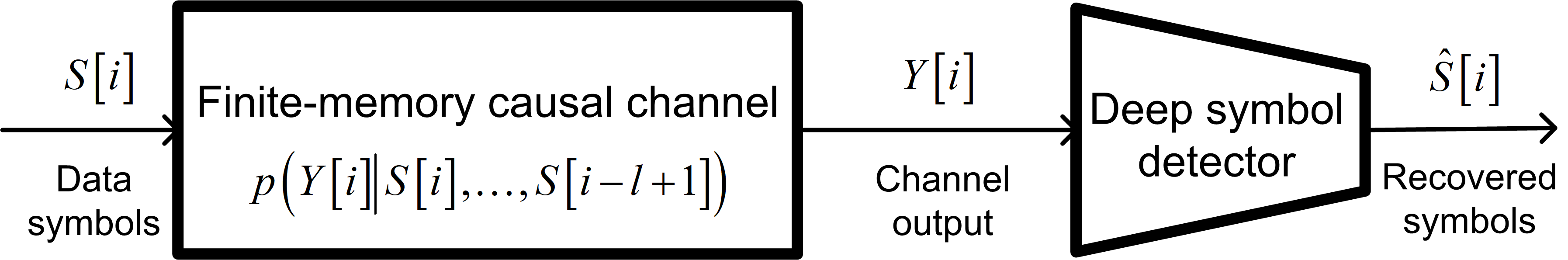
Figure 1: System model.

Our goal is to design a DNN architecture for recovering ${\boldsymbol{S}}^{t}$ from the channel output ${\boldsymbol{Y}}^{t}$. In particular, in our model the receiver assumes that the channel is stationary, causal, and has finite memory $l$, namely, that the input-output statistical relationship is of the form (1). The receiver also knows the constellation $\mathcal{S}$. We do not assume that the receiver knows the conditional PDF $p_{{Y[i]|{\boldsymbol{S}}_{i\!-\!l\!+\!1}^{i}}}\left(y|{\boldsymbol{s}}\right)$, i.e., the receiver does not have this CSI. The optimal detector for finite-memory channels, based on which we design our network, is the Viterbi algorithm [1]. Therefore, as a preliminary step to designing the DNN, we review Viterbi detection in the following subsection.

II-B The Viterbi Detection Algorithm

The following description of the Viterbi algorithm is based on [26, Ch. 3.4]. Since the constellation points are equiprobable, the optimal decision rule in the sense of minimal probability of error is the maximum likelihood decision rule, namely, for a given channel output ${\boldsymbol{y}}^{t}$, the estimated output is given by

$$\hat{{\boldsymbol{s}}}^{t}\left({\boldsymbol{y}}^{t}\right) \triangleq\mathop{\arg\max}_{{\boldsymbol{s}}^{t}\in\mathcal{S}^{t}}p_{{{\boldsymbol{Y}}^{t}|{\boldsymbol{S}}^{t}}}\left({{\boldsymbol{y}}^{t}|{\boldsymbol{s}}^{t}}\right)$$

$$=\mathop{\arg\min}_{{\boldsymbol{s}}^{t}\in\mathcal{S}^{t}}-\log p_{{{\boldsymbol{Y}}^{t}|{\boldsymbol{S}}^{t}}}\left({\boldsymbol{y}}^{t}|{\boldsymbol{s}}^{t}\right).$$ (2)

By defining

$$c_{i}\left({\boldsymbol{s}}\right)\triangleq-\log p_{{{\boldsymbol{Y}}[i]|{\boldsymbol{S}}_{i-l+1}^{i}}}\left({\boldsymbol{y}}[i]|{\boldsymbol{s}}\right),\qquad{\boldsymbol{s}}\in\mathcal{S}^{l},$$ (3)

it follows from (1) that the log-likelihood function in (2) can be written as

$$\log p_{{{\boldsymbol{Y}}^{t}|{\boldsymbol{S}}^{t}}}\left({\boldsymbol{y}}^{t}|{\boldsymbol{s}}^{t}\right)=\sum\limits_{i=1}^{t}c_{i}\left({\boldsymbol{s}}_{i-l+1}^{i}\right),$$ (4)

and the optimization problem (2) becomes

$$\hat{{\boldsymbol{s}}}^{t}\left({\boldsymbol{y}}^{t}\right) =\mathop{\arg\min}_{{\boldsymbol{s}}^{t}\in\mathcal{S}^{t}}\sum\limits_{i=1}^{t}c_{i}\left({\boldsymbol{s}}_{i-l+1}^{i}\right).$$ (5)

The optimization problem (5) can be solved recursively using dynamic programming, by treating the possible combinations of transmitted symbols at each time instance as states and iteratively updating a path cost value for each state, The resulting recursive solution, which is known as the Viterbi algorithm, is given below as Algortihm 1.

Algorithm 1 The Viterbi Algorithm

1:  Input: Block of channel outputs ${\boldsymbol{y}}^{t}$, where $t>l$.

2:  Initialization: Set $k=1$, and fix the initial path cost $\tilde{c}_{0}\left(\tilde{{\boldsymbol{s}}}\right)=0$, for each state $\tilde{{\boldsymbol{s}}}\in\mathcal{S}^{l}$.

3:   For each state $\tilde{{\boldsymbol{s}}}\in\mathcal{S}^{l}$, compute the path cost via $\tilde{c}_{k}\left(\tilde{{\boldsymbol{s}}}\right)=\mathop{\min}\limits_{{\boldsymbol{u}}\in\mathcal{S}^{l}:{\boldsymbol{u}}_{2}^{l}=\tilde{{\boldsymbol{s}}}^{l-1}}\left(\tilde{c}_{k-1}\left({\boldsymbol{u}}\right)+{c}_{k}\left(\tilde{{\boldsymbol{s}}}\right)\right)$.

4:  If $k\geq l$, set $\left(\hat{{\boldsymbol{s}}}\right)_{k\!-\!l\!+\!1}\!:=\!\left(\tilde{{\boldsymbol{s}}}_{k}^{\rm o}\right)_{1}$, where $\tilde{{\boldsymbol{s}}}^{\rm o}_{k}\!=\!\mathop{\arg\min}\limits_{\tilde{{\boldsymbol{s}}}\in\mathcal{S}^{l}}\tilde{c}_{k}\left(\tilde{{\boldsymbol{s}}}\right)$.

5:  Set $k:=k+1$. If $k\leq t$ go to Step 3.

6:  Output: decoded output $\hat{{\boldsymbol{s}}}^{t}$, where $\hat{{\boldsymbol{s}}}_{t-l+1}^{t}:=\tilde{{\boldsymbol{s}}}_{{t}}^{\rm o}$.

In addition to its ability to achieve the minimal error probability [2], the Viterbi algorithm has several major advantages:

1. The algorithm solves (2) at a computational complexity that is linear in the blocklength $t$. For comparison, the computational complexity of solving (2) directly grows exponentially with $t$.

2. The algorithm produces estimates sequentially on run-time. In particular, while in (2) the estimated output $\hat{{\boldsymbol{s}}}^{t}$ is computed using the entire received block ${\boldsymbol{y}}^{t}$, Algorithm 1 computes $\hat{s}[i]$ once $y[i+l-1]$ is received.

In order to implement Algorithm 1, one must be able to compute ${c}_{i}\left({{\boldsymbol{s}}}\right)$ of (3) for all $i\in\mathcal{T}$ and for each ${\boldsymbol{s}}\in\mathcal{S}^{l}$. Consequently, the conditional PDF of the channel, which we refer to as full CSI, must be explicitly known. As discussed in the introduction, obtaining full CSI may be extremely difficult in rapidly changing channels and may also require a large training overhead. In the following section we propose ViterbiNet, an ML-based symbol decoder based on the Viterbi algorithm, that does not require CSI.

III ViterbiNet

III-A Integrating ML into the Viterbi Algorithm

In order to integrate ML into the Viterbi Algorithm, we note that CSI is required in Algorithm 1 only in Step 3 to compute the log-likelihood function $c_{i}({\boldsymbol{s}})$. Once $c_{i}({\boldsymbol{s}})$ is computed for each ${\boldsymbol{s}}\in\mathcal{S}^{l}$, the Viterbi algorithm only requires knowledge of the memory length $l$ of the channel. This requirement is much easier to satisfy compared to knowledge of the exact channel input-output statistical relationship, i.e., full CSI. In fact, a common practice when using the model-based Viterbi algorithm is to limit the channel memory by filtering the channel output prior to symbol detection [27] in order to reduce computational complexity. The approach in [27], which assumes that the channel is modeled as a linear time-invariant (LTI) filter, is an example of how the channel memory used by the algorithm can be fixed in advance, regardless of the true memory length of the underlying channels. Furthermore, estimating the channel memory in a data-driven fashion without a-priori knowledge of the underlying model is a much simpler task compared to symbol detection, and can be reliably implemented using standard correlation peak based estimators, see, e.g., [28]. We henceforth assume that the receiver has either accurate knowledge or a reliable upper bound on $l$, and leave the extension of the decoder to account for unknown memory length to future exploration.

Since the channel is stationary, it holds by (3) that if $y[i]=y[k]$ then $c_{i}({\boldsymbol{s}})=c_{k}({\boldsymbol{s}})$, for each ${\boldsymbol{s}}\in\mathcal{S}^{l}$, and $i,k\in\mathcal{T}$. Consequently, the log-likelihood function $c_{i}({\boldsymbol{s}})$ depends only on the values of $y[i]$ and of ${\boldsymbol{s}}$, and not on the time index $i$. Therefore, in our proposed structure we replace the explicit computation of the log-likelihood (3) with an ML-based system that learns to evaluate the cost function from the training data. In this case, the input of the system is $y[i]$ and the output is an estimate of $c_{i}({{\boldsymbol{s}}})$, denoted $\hat{c}_{i}({{\boldsymbol{s}}})$, for each ${\boldsymbol{s}}\in\mathcal{S}^{l}$. The rest of the Viterbi algorithm remains intact, namely, the detector implements Algorithm 1 while using ML techniques to compute the log-likelihood function $c_{i}({{\boldsymbol{s}}})$. The proposed architecture is illustrated in Fig. 2.

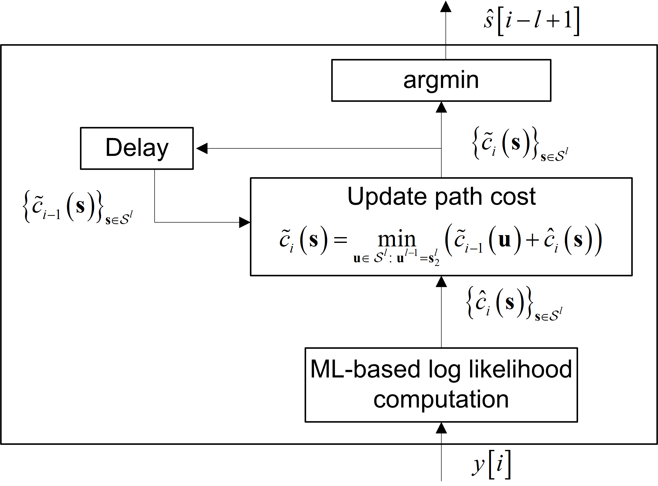
Figure 2: Proposed DNN-based Viterbi decoder.

A major challenge in implementing a network capable of computing $c_{i}({\boldsymbol{s}})$ from $y[i]$ stems from the fact that, by (3), $c_{i}({\boldsymbol{s}})$ represents the log-likelihood of $Y[i]=y[i]$ given ${\boldsymbol{S}}_{i-l+1}^{i}={\boldsymbol{s}}$. However, DNNs trained to minimize the cross entropy loss typically output the conditional distribution of ${\boldsymbol{S}}_{i-l+1}^{i}={\boldsymbol{s}}$ given $Y[i]=y[i]$, i.e., $p_{{{\boldsymbol{S}}_{i-l+1}^{i}|Y[i]}}\left({\boldsymbol{s}}|y[i]\right)$. Specifically, classification DNNs with input $Y[i]=y[i]$, which typically takes values in a discrete set, or alternatively, is discretized by binning a continuous quantity as in [30, 29], output the distribution of the label ${\boldsymbol{S}}_{i-l+1}^{i}$ conditioned on that input $Y[i]=y[i]$, and not the distribution of the input conditioned on all possible values of the label ${\boldsymbol{S}}_{i-l+1}^{i}$. For this reason, the previous work [15] used a DNN to approximate the MAP detector by considering $p_{{S[i]|{\boldsymbol{Y}}_{i-l+1}^{i}}}\left(s|{\boldsymbol{y}}_{i-l+1}^{i}\right)$. It is emphasized that the quantity which is needed for the Viterbi algorithm is the conditional PDF $p_{{Y[i]|{\boldsymbol{S}}_{i-l+1}^{i}}}\left(y[i]|{\boldsymbol{s}}\right)$, and not the conditional distribution $p_{{{\boldsymbol{S}}_{i-l+1}^{i}|Y[i]}}\left({\boldsymbol{s}}|y[i]\right)$. Note, for example, that while $\sum_{{\boldsymbol{s}}\in\mathcal{S}^{l}}p_{{{\boldsymbol{S}}_{i-l+1}^{i}|Y[i]}}\left({\boldsymbol{s}}|y[i]\right)=1$, for the desired conditional PDF $\sum_{{\boldsymbol{s}}\in\mathcal{S}^{l}}p_{{Y[i]|{\boldsymbol{S}}_{i-l+1}^{i}}}\left(y[i]|{\boldsymbol{s}}\right)\neq 1$ in general. Therefore, outputs generated using conventional DNNs with a softmax output layer are not applicable. The fact that Algorithm 1 specifically uses the conditional PDF $p_{{Y[i]|{\boldsymbol{S}}_{i-l+1}^{i}}}\left(y[i]|{\boldsymbol{s}}\right)$ instead of $p_{{{\boldsymbol{S}}_{i-l+1}^{i}|Y[i]}}\left({\boldsymbol{s}}|y[i]\right)$ allows it to exploit the Markovian nature of the channel, induced by the finite memory in (1), resulting in the advantages A1-A2 discussed in Subsection II-B.

In order to tackle this difficulty, we recall that by Bayes’ theorem, as the channel inputs are equiprobable, the desired conditional PDF $p_{{Y[i]|{\boldsymbol{S}}_{i-l+1}^{i}}}\left(y|{\boldsymbol{s}}\right)$ can be written as

$$p_{{Y[i]|{\boldsymbol{S}}_{i-l+1}^{i}}}\left(y|{\boldsymbol{s}}\right)=\frac{p_{{{\boldsymbol{S}}_{i-l+1}^{i}|Y[i]}}\left({\boldsymbol{s}}|y\right)\cdot p_{{Y[i]}}(y)}{m^{-l}}.$$ (6)

Therefore, given estimates of $p_{{Y[i]}}(y[i])$ and of $p_{{{\boldsymbol{S}}_{i-l+1}^{i}|Y[i]}}\left({\boldsymbol{s}}|y[i]\right)$ for each ${\boldsymbol{s}}\in\mathcal{S}^{l}$, the log-likelihood function $c_{i}({\boldsymbol{s}})$ can be recovered using (6) and (3).

A parametric estimate of $p_{{{\boldsymbol{S}}_{i-l+1}^{i}|Y[i]}}\left({\boldsymbol{s}}|y[i]\right)$, denoted $\hat{p}_{{{\boldsymbol{\theta}}}}\left({\boldsymbol{s}}|y[i]\right)$, can be reliably obtained from training data using standard classification DNNs with a softmax output layer. The marginal PDF of $Y[i]$ may be estimated from the training data using conventional kernel density estimation methods [31]. Furthermore, the fact that $Y[i]$ is a stochastic mapping of ${\boldsymbol{S}}_{i-l+1}^{i}$ implies that its distribution can be approximated as a mixture model of $m^{l}$ kernel functions [32]. Consequently, a parametric estimate of $p_{{Y[i]}}(y[i])$, denoted $\hat{p}_{{{\boldsymbol{\varphi}}}}\left(y[i]\right)$, can be obtained from the training data using mixture density networks [34], expectation minimization (EM)-based algorithms [32, Ch. 2], or any other finite mixture model fitting method. The resulting ML-based log-likelihood computation is illustrated in Fig. 3.

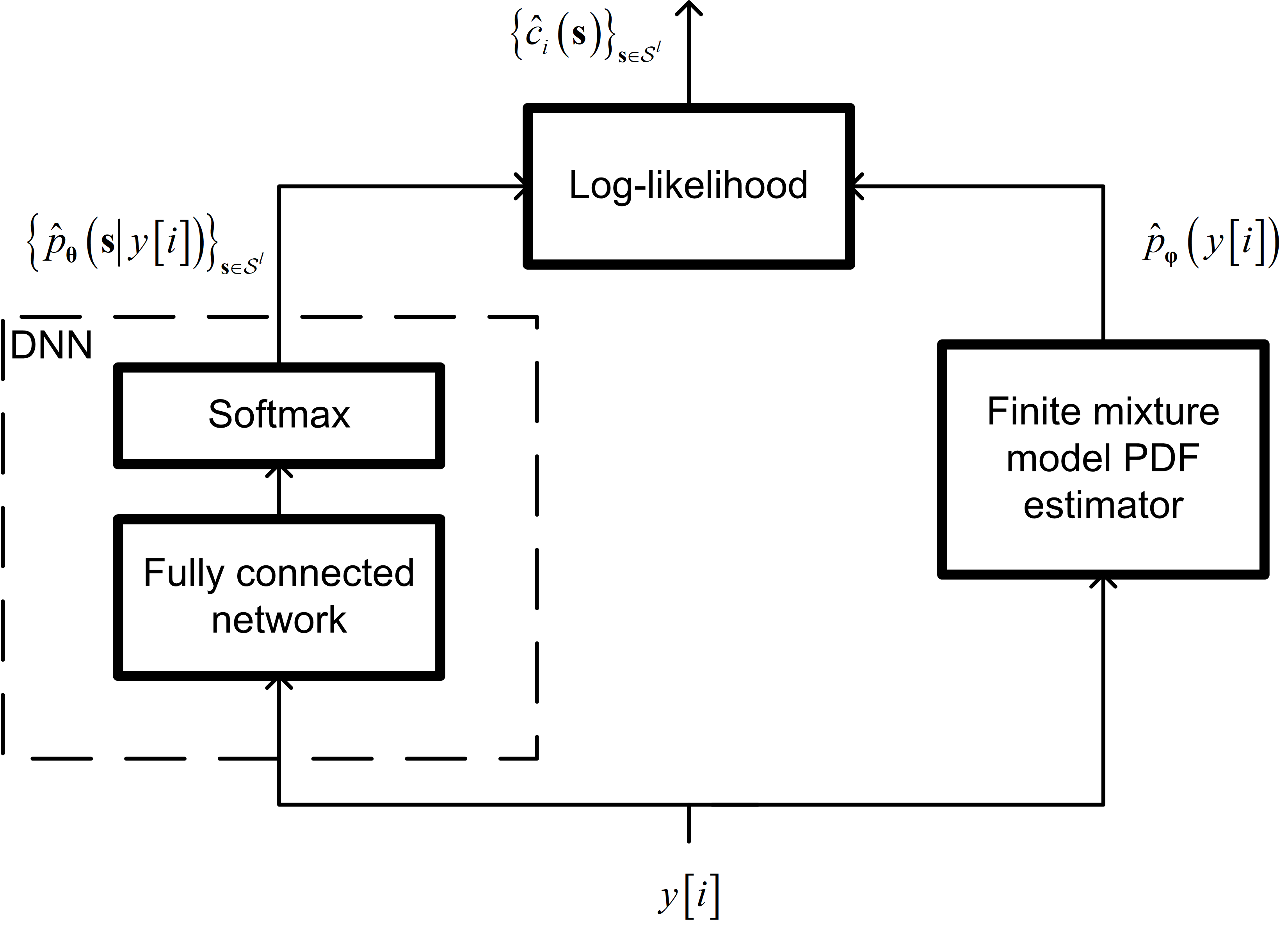
Figure 3: ML-based log-likelihood computation.

The ML-based log-likelihood computation depicted in Fig. 3 is applicable for both real-valued channels, where $\mathcal{Y}$ and $\mathcal{S}$ are subsets of $\mathcal{R}$, as well as complex channels, in which the elements of $\mathcal{Y}$ and $\mathcal{S}$ take complex values. In particular, for complex-valued channels, the input to the classification DNN should be a real vector consisting of the real and imaginary parts of $y[i]$, as DNNs typically operate on real-valued quantities. Furthermore, the finite mixture model PDF estimator should use kernel functions for complex distributions, e.g., complex Gaussian mixture. Except for these modifications, the architecture of ViterbiNet is invariant as to whether the channel is real or complex-valued.

III-B Discussion

The architecture of ViterbiNet is based on the Viterbi algorithm, which achieves the minimal probability of error for communications over finite-memory causal channels. Since ViterbiNet is data-driven, it learns the log-likelihood function from training data without requiring full CSI. When properly trained, the proposed DNN is therefore expected to approach the performance achievable with the conventional CSI-based Viterbi algorithm, as numerically demonstrated in Section V. Unlike direct applications of classification DNNs, which produce a parametric estimate of the conditional distribution of the transmitted symbols given the channel output, ViterbiNet is designed to estimate the conditional distribution of the channel output given the transmitted symbols. This conditional distribution, which encapsulates the Markovian structure of finite-memory channels, is then used to obtain the desired log-likelihoods, as discussed in the previous subsection. The estimation of these log-likelihoods, which are not obtained by simply applying a classification DNN to the channel output, is then exploited to recover the transmitted symbols using the same operations carried out by the conventional Viterbi algorithm.

ViterbiNet replaces the CSI-based parts of the Viterbi algorithm with an ML-based scheme. Since this aspect of the channel model is relatively straightforward to learn, ViterbiNet can utilize a simple and standard DNN architecture. The simple DNN structure implies that the network can be trained quickly with a relatively small number of training samples, as also observed in the numerical study in Section V. This indicates the potential of the proposed architecture to adapt on runtime to channel variations with minimal overhead, possibly using pilot sequences periodically embedded in the transmitted frame for online training.

The approach used in designing ViterbiNet, namely, maintaining the detection scheme while replacing its channel-model-based computations with dedicated ML methods, can be utilized for implementing additional algorithms in communications and signal processing in a data-driven manner. For instance, in [35], we showed how this approach can allow a MIMO receiver to learn to implement the soft iterative interference cancellation scheme of [36] from a small training set. In particular, the ML-based computation of the conditional probability used in ViterbiNet to carry out Viterbi detection can be utilized to realize other trellis or factor graph based detection schemes, such as the BCJR algorithm [37], by properly modifying the processing of these estimates. We leave the study of these alternative data-driven schemes for future investigation.

The fact that ViterbiNet is based on the Viterbi algorithm implies that it also suffers from some of its drawbacks. For example, when the constellation size $m$ and the channel memory $l$ grow large, the Viterbi algorithm becomes computationally complex due to the need to compute the log-likelihood for each of the possible $m^{l}$ different values of ${\boldsymbol{s}}$. Consequently, the complexity of ViterbiNet is expected to grow exponentially as $m$ and $l$ grow, since the label space of the DNN grows exponentially. It is noted that greedy schemes for reducing the complexity of the Viterbi algorithm, such as beam search [38] and reduced-state equalization [39], were shown to result in minimal performance degradation, and we thus expect that these methods can inspire similar modifications to ViterbiNet, facilitating its application with large $m$ and $l$. We leave the research into reducing the complexity of ViterbiNet through such methods to future investigation.

IV Extension to Block-Fading Channels

A major challenge associated with using ML algorithms in communications stems from the fact that, in order to exploit the ability of DNNs to learn an underlying model, the network should operate under the same (or a closely resembling) statistical relationship for which it was trained. Many communication channels, and particularly wireless channels, are dynamic by nature, and are commonly modeled as block-fading [40]. In such channels, each transmitted block may undergo a different statistical transformation. In Section V, we show that ViterbiNet is capable of achieving relatively good performance when trained using samples taken from a variety of channels rather than from the specific channel for which it is tested. Consequently, a possible approach to use ViterbiNet in block-fading channels is to train the system using samples acquired from a large variety of channels. However, such an approach requires a large amount of training data in order to cover a multitude of different channel conditions, and is also expected to result in degraded performance, especially when tested under a channel model that deviates significantly from the channels used during training. This motivates us to extend ViterbiNet by allowing the receiver to track and adjust to time-varying channel conditions in real-time, by exploiting the inherent structure of digital communication signals and, particularly, of coded communications. Broadly speaking, we utilize the fact that in coded systems, the receiver is capable of identifying and correcting symbol detection errors. The identification and correction of these errors can be used to retrain ViterbiNet online using meta-learning principles [24], allowing it to track channel variations. To present this approach, we first extend the channel model of Subsection IV-A to account for coded communications and block-fading channels. Then, we detail in Subsection IV-B how ViterbiNet can exploit the use of channel coding for online training.

IV-A Coded Communications over Block-Fading Channels

In coded communications, each block of $t$ transmitted channel symbols represents a channel codeword conveying $b$ bits. During the $j$th block, $j\in\mathcal{N}$, a vector of bits, denoted ${\boldsymbol{B}}^{b}_{(j)}\in\{0,1\}^{b}$, is encoded and modulated into the symbol vector ${\boldsymbol{S}}^{t}_{(j)}$ which is transmitted over the channel. The purpose of such channel coding is to facilitate the recovery of the information bits at the receiver. A channel code can consist of both FEC codes, such as Reed-Solomon (RS) codes, as well as error detection codes, such as checksums and cyclic redundancy checks. The receiver uses the recovered symbols $\hat{{\boldsymbol{S}}}^{t}_{(j)}$ to decode the information bits $\hat{{\boldsymbol{B}}}^{b}_{(j)}\in\{0,1\}^{b}$. The presence of FEC codes implies that even when some of the symbols are not correctly recovered, i.e., ${\boldsymbol{S}}^{t}_{(j)}\neq\hat{{\boldsymbol{S}}}^{t}_{(j)}$, the information bits can still be perfectly decoded. Error detection codes allow the receiver to detect whether the information bits were correctly recovered and estimate the number of bit errors, i.e., the Hamming distance between ${\boldsymbol{B}}^{b}_{(j)}$ and $\hat{{\boldsymbol{B}}}^{b}_{(j)}$, denoted $\epsilon_{(j)}$.

In block-fading channels, each block of transmitted channel symbols undergoes a different channel. In particular, for the $j$th block, $j\in\mathcal{N}$, the conditional distribution of the channel output ${\boldsymbol{Y}}^{t}_{(j)}$ given the input ${\boldsymbol{S}}^{t}_{(j)}$ represents a finite-memory causal stationary channel as described in Subsection II-A. However, this conditional distribution can change between different blocks, namely, it depends on the block index $j$. An illustration of this channel model is depicted in Fig. 4. Block-fading channels model dynamic environments in which the transmitted bursts are shorter than the coherence duration of the channel, faithfully representing many scenarios of interest in wireless communications [40].

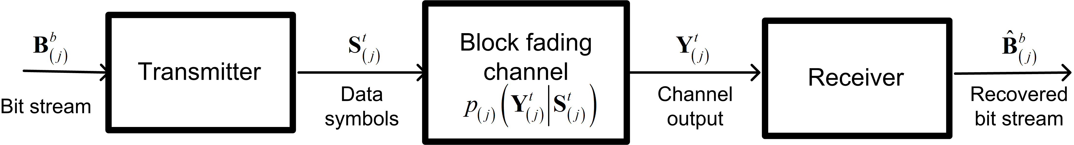
Figure 4: Coded communications over block-fading channels.

Since each block undergoes a different channel input-output relationship, the receiver must be able to track and adapt to the varying channel conditions in order to optimize its performance. In the next subsection, we show how the fact that ViterbiNet requires relatively small training sets can be combined with the presence of coded communications such that the receiver can track channel variations online.

IV-B ViterbiNet with Online Training

We next discuss how coded communications can allow ViterbiNet to train and track channel variations online. Our proposed approach is inspired by concepts from meta-learning [24], which is a field of research focusing on self-teaching ML algorithms, as well as from decision-directed adaptive filter theory, which considers the blind adaptation of adjustable filters based on some decision mechanism, see, e.g., [41].

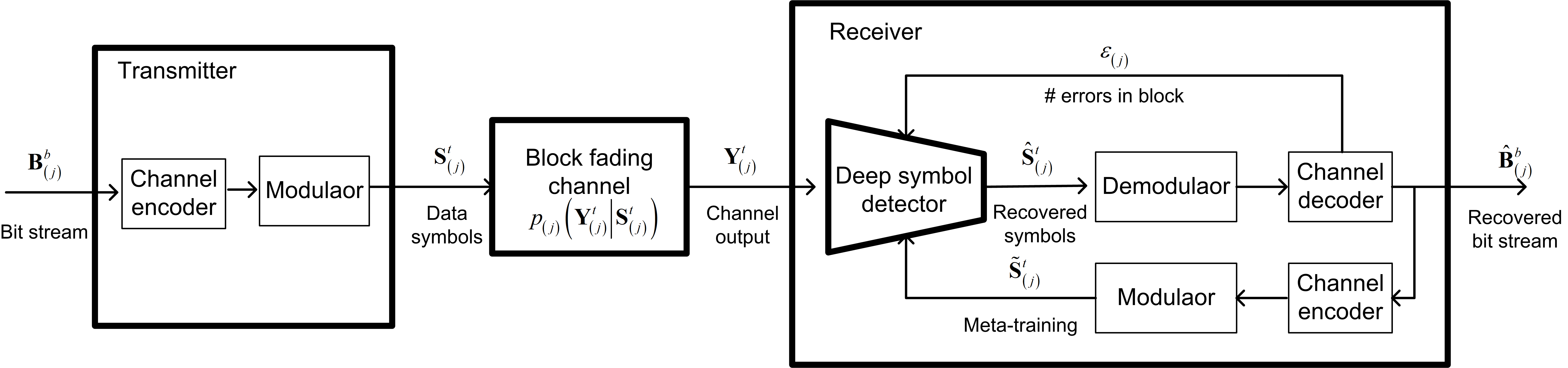
Figure 5: Online training model.

ViterbiNet uses the channel outputs over a single block, denoted ${\boldsymbol{Y}}^{t}_{(j)}$, where $j\in\mathcal{N}$ represents the block index, to generate an estimate of the transmitted symbols, denoted $\hat{{\boldsymbol{S}}}^{t}_{(j)}$. In the presence of FEC codes, when the number of detection errors is not larger than the minimal distance of the code, the encoded bits can still be perfectly recovered [42, Ch. 8]. It therefore follows that when the symbol error rate (SER) of ViterbiNet is small enough such that the FEC code is able to compensate for these errors, the transmitted message can be recovered. The recovered message may also be re-encoded to generate new training samples, denoted $\tilde{{\boldsymbol{S}}}^{t}_{(j)}$, referred to henceforth as meta-training. If indeed the encoded bits were successfully recovered, then $\tilde{{\boldsymbol{S}}}^{t}_{(j)}$ represents the true channel input from which ${\boldsymbol{Y}}^{t}_{(j)}$ was obtained. Consequently, the pair $\tilde{{\boldsymbol{S}}}^{t}_{(j)}$ and ${\boldsymbol{Y}}^{t}_{(j)}$ can be used to re-train ViterbiNet. The simple DNN structure used in ViterbiNet implies that it can be efficiently and quickly retrained with a relatively small number of training samples, such as the size of a single transmission block in a block-fading channel. An illustration of the proposed online training mechanism is depicted in Fig. 5.

A natural drawback of decision-directed approaches is their sensitivity to decision errors. For example, if the FEC decoder fails to successfully recover the encoded bits, then the meta-training samples $\tilde{{\boldsymbol{S}}}^{t}_{(j)}$ do not accurately represent the channel input resulting in ${\boldsymbol{Y}}^{t}_{(j)}$. In such cases, the inaccurate training sequence may gradually deteriorate the recovery accuracy of the re-trained ViterbiNet, making the proposed approach unreliable, particularly in low signal-to-noise ratios where decoding errors occur frequently. Nonetheless, when error detection codes are present in addition to FEC codes, the effect of decision errors can be mitigated. In particular, when the receiver has a reliable estimate of $\epsilon_{(j)}$, namely, the number of bit errors in decoding the $j$th block, it can decide to generate meta-training and re-train the symbol detector only when the number of errors is smaller than some threshold $\bar{\epsilon}$. Using this approach, only accurate meta-training is used, and the effect of decision errors can be mitigated and controlled. The proposed online training mechanism is summarized below as Algorithm 2.

Algorithm 2 Online Training of ViterbiNet

1:  Input: Block of channel outputs ${\boldsymbol{y}}^{t}$; ViterbiNet DNN weights ${\boldsymbol{\theta}}$ and mixture model parameters ${\boldsymbol{\varphi}}$; Bit error threshold $\bar{\epsilon}$.

2:   Apply ViterbiNet with parameters ${\boldsymbol{\theta}},{\boldsymbol{\varphi}}$ to recover the symbols $\hat{{\boldsymbol{s}}}^{t}$ from ${\boldsymbol{y}}^{t}$.

3:  Decode bits vector $\hat{{\boldsymbol{b}}}^{b}$ and number of error $\epsilon$ from $\hat{{\boldsymbol{s}}}^{t}$.

4:  if  $\epsilon<\bar{\epsilon}$ then

5:     Encode and modulate $\hat{{\boldsymbol{b}}}^{b}$ into $\tilde{{\boldsymbol{s}}}^{t}$.

6:      Re-train DNN weights ${\boldsymbol{\theta}}$ using meta-training $\left(\tilde{{\boldsymbol{s}}}^{t},{\boldsymbol{y}}^{t}\right)$.

7:      Update mixture model ${\boldsymbol{\varphi}}$ using ${\boldsymbol{y}}^{t}$.

8:  end if

9:  Output: Decoded bits $\hat{{\boldsymbol{b}}}^{b}$; ViterbiNet DNN weights ${\boldsymbol{\theta}}$ and mixture model parameters ${\boldsymbol{\varphi}}$.

Setting the value of $\bar{\epsilon}$ should be based on the nature of the expected variations between blocks as well as on the FEC scheme. When operating with gradual variations, one can set $\bar{\epsilon}$ to represent zero errors, guaranteeing that the meta-training symbols used for re-training ViterbiNet are accurate. However, this setting may limit the ability of ViterbiNet to track moderate channel variations. Using larger values of $\bar{\epsilon}$ should also account for the FEC method used, as for some codes, encoding a bit stream with a small number of errors may result in a distant codeword compared to the one transmitted, thus yielding inaccurate meta-training labels. In Subsection V-B we numerically evaluate the effect of different values of $\bar{\epsilon}$ on the ability of ViterbiNet to reliably track block-fading channels.

The learning rate used in re-training the DNN in Step 6 of Algorithm 2 should be set based on the expected magnitude of the channel variations. Specifically, the value of the learning rate balances the contributions of the initial DNN weights, which were tuned based on a past training set corresponding to previous channel realizations, and that of the typically much smaller meta-training set, representing the current channel. Using larger learning rates implies that the network can adapt to nontrivial channel variations, but also increases the sensitivity of the algorithm to decision errors, and should thus be used with smaller values of the threshold $\bar{\epsilon}$.

The method for updating the mixture model parameters ${\boldsymbol{\varphi}}$ in Step 7 of Algorithm 2 depends on which of the possible finite mixture model estimators discussed in Subsection III-A is used. For example, when using EM-based model fitting, the previous model parameters ${\boldsymbol{\varphi}}$ can be used as the initial guess used for fitting the PDF based on the current channel outputs.

Finally, we note that our meta-learning based online training scheme exploits only the structure induced by channel codes. Modern communication protocols dictate a multitude of additional structures that can be exploited to generate meta-training. For example, many communication protocols use a-priori known preamble sequences to facilitate synchronization between the communicating nodes [42, Ch. 14.2]. The receiver can thus use the a-priori knowledge of the preamble to generate meta-training from the corresponding channel outputs, which can be used for re-training ViterbiNet online. Additional structures induced by protocols that can be exploited to re-train ViterbiNet in a similar manner include specific header formats, periodic pilots, and network management frames. Consequently, while the proposed approach focuses on using channel codes to generate meta-training, it can be extended to utilize various other inherent structures of digital communication signals.

V Numerical Study

In this section we numerically evaluate the performance of ViterbiNet. In particular, we first consider time-invariant channels in Subsection V-A. For such setups, we numerically compare the performance of ViterbiNet to the conventional model-based Viterbi algorithm as well as to previously proposed deep symbol detectors, and evaluate the resiliency of ViterbiNet to inaccurate training. Then, we consider block-fading channels, and evaluate the performance of ViterbiNet with online training in Subsection V-B. In the following we assume that the channel memory $l$ is a-priori known. It is emphasized that for all the simulated setups we were able to accurately detect the memory length using a standard correlation peak based estimator, see, e.g., [28], hence this assumption is not essential. Throughout this numerical study we implement the fully connected network in Fig. 3 using three layers: a $1\times 100$ layer followed by a $100\times 50$ layer and a $50\times 16(=|m|^{l})$ layer, using intermediate sigmoid and ReLU activation functions, respectively. The mixture model estimator approximates the distribution as a Gaussian mixture using EM-based fitting [32, Ch. 2]. The network is trained using $5000$ training samples to minimize the cross-entropy loss via the Adam optimizer [43] with learning rate $0.01$, using up to $100$ epochs with mini-batch size of $27$ observations. We note that the number of training samples is of the same order and even smaller compared to typical preamble sequences in wireless communications. Due to the small number of training samples and the simple architecture of the DNN, only a few minutes are required to train the network on a standard CPU.

V-A Time-Invariant Channels

We first consider two finite-memory causal scalar channels: An intersymbol interference (ISI) channel with additive white Gaussian noise (AWGN), and a Poisson channel. In both channels we set the memory length to $l=4$. For the ISI channel with AWGN, we let $W[i]$ be a zero-mean unit variance AWGN independent of $S[i]$, and let ${\boldsymbol{h}}(\gamma)\in\mathcal{R}^{l}$ be the channel vector representing an exponentially decaying profile given by $\left({\boldsymbol{h}}\right)_{\tau}\triangleq e^{-\gamma(\tau-1)}$ for $\gamma>0$. The input-output relationship is given by

$$Y[i]=\sqrt{\rho}\cdot\sum\limits_{\tau=1}^{l}\left({\boldsymbol{h}}(\gamma)\right)_{\tau}S[i-\tau+1]+W[i],$$ (7)

where $\rho>0$ represents the SNR. Note that even though the effect of the ISI becomes less significant as $\gamma$ grows, the channel (7) has memory length of $l=4$ for all values of $\gamma$ considered in this study. The channel input is randomized from a binary phase shift keying constellation, i.e., $\mathcal{S}=\{-1,1\}$. For the Poisson channel, the channel input represents on-off keying, namely, $\mathcal{S}=\{0,1\}$, and the channel output $Y[i]$ is generated from the input via

$$Y[i]|{\boldsymbol{S}}^{t}\sim\mathds{P}\left(\sqrt{\rho}\cdot\sum\limits_{\tau=1}^{l}\left({\boldsymbol{h}}(\gamma)\right)_{\tau}S[i-\tau+1]+1\right),$$ (8)

where $\mathds{P}(\lambda)$ is the Poisson distribution with parameter $\lambda>0$.

For each channel, we numerically compute the SER of ViterbiNet for different values of the SNR parameter $\rho$. In the following study, the DNN is trained anew for each value of $\rho$. For each SNR $\rho$, the SER values are averaged over $20$ different channel vectors ${\boldsymbol{h}}(\gamma)$, obtained by letting $\gamma$ vary in the range $[0.1,2]$. For comparison, we numerically compute the SER of the Viterbi algorithm, as well as that of the sliding bidirectional (SBRNN) deep symbol decoder proposed in [15]. In order to study the resiliency of ViterbiNet to inaccurate training, we also compute the performance when the receiver only has access to a noisy estimate of ${\boldsymbol{h}}(\gamma)$, and specifically, to a copy of ${\boldsymbol{h}}(\gamma)$ whose entries are corrupted by i.i.d. zero-mean Gaussian noise with variance $\sigma_{e}^{2}$. In particular, we use $\sigma_{e}^{2}=0.1$ for the Gaussian channel (7), and $\sigma_{e}^{2}=0.08$ for the Poisson channel (8). We consider two cases: Perfect CSI, in which the channel-model-based Viterbi detector has accurate knowledge of ${\boldsymbol{h}}(\gamma)$, while ViterbiNet is trained using labeled samples generated with the same ${\boldsymbol{h}}(\gamma)$ used for generating the test data; and CSI uncertainty, where the Viterbi algorithm implements Algorithm 1 with the log-likelihoods computed using the noisy version of ${\boldsymbol{h}}(\gamma)$, while the labeled data used for training ViterbiNet is generated with the noisy version of ${\boldsymbol{h}}(\gamma)$ instead of the true one. In particular, for CSI uncertainty, the $5000$ samples used for training ViterbiNet are divided into $10$ subsets, each generated from a channel with a different realization of the noise in ${\boldsymbol{h}}(\gamma)$. In all cases, the information symbols are uniformly randomized in an i.i.d. fashion from $\mathcal{S}$, and the test samples are generated from their corresponding channel, i.e., (7) and (8) for the Gaussian and Poisson channels, respectively, with the true channel vector ${\boldsymbol{h}}(\gamma)$.

The numerically computed SER values, averaged over $50000$ Monte Carlo simulations, versus $\rho\in[-6,10]$ dB for the ISI channel with AWGN are depicted in Fig. 6, while the corresponding performance versus $\rho\in[10,34]$ dB for the Poisson channel are depicted in Fig. 7. Observing Figs. 6-7, we note that the performance of ViterbiNet approaches that of the conventional CSI-based Viterbi algorithm. In particular, for the AWGN case, in which the channel output obeys a Gaussian mixture distribution, the performance of ViterbiNet coincides with that of the Viterbi algorithm, while for the Poisson channel a very small gap is observed at high SNRs due to the model mismatch induced by approximating the distribution of $Y[i]$ as a Gaussian mixture. We expect the performance of ViterbiNet to improve in that scenario when using a Poisson kernel density estimator for $\hat{p}_{{{\boldsymbol{\varphi}}}}\left(y[i]\right)$, however, this requires some basic level of knowledge of the input-output relationship. It is also observed in Figs. 6-7 that the SBRNN receiver, which was shown in [15] to approach the performance of the CSI-based Viterbi algorithm when sufficient training is provided, is outperformed by ViterbiNet here due to the small amount of training data provided. For example, for the ISI channel with AWGN, both the Viterbi detector as well as ViterbiNet achieve an SER of $4.7\cdot 10^{-3}$ for SNR of $8$ dB, while the SBRNN detector achieves an SER of $8.5\cdot 10^{-3}$ for the same SNR value. For the Poisson channel at an SNR of $28$ dB, the Viterbi algorithm achieves an SER of $5.1\cdot 10^{-3}$, while ViterbiNet and the SBRNN detector achieve SER values of $6.6\cdot 10^{-3}$ and $8.3\cdot 10^{-3}$, respectively. These results demonstrate that ViterbiNet, which uses simple DNN structures embedded into the Viterbi algorithm, requires significantly less training compared to previously proposed ML-based receivers.

In the presence of CSI uncertainty, it is observed in Figs. 6-7 that ViterbiNet significantly outperforms the Viterbi algorithm. In particular, when ViterbiNet is trained with a variety of different channel conditions, it is still capable of achieving relatively good SER performance under each of the channel conditions for which it is trained, while the performance of the conventional Viterbi algorithm is significantly degraded in the presence of imperfect CSI. While the SBRNN receiver is shown to be more resilient to inaccurate CSI compared to the Viterbi algorithm, as was also observed in [15], it is outperformed by ViterbiNet with the same level of uncertainty, and the performance gap is more notable in the AWGN channel. The reduced gain of ViterbiNet over the SBRNN receiver for the Poisson channel stems from the fact that ViterbiNet here uses a Gaussian mixture kernel density estimator for the PDF of $Y[i]$, which obeys a Poisson mixture distribution for the Poisson channel (8).

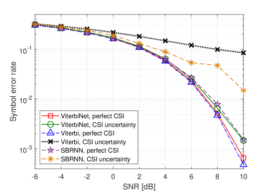
Figure 6: SER versus SNR, ISI channel with AWGN.

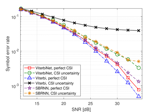
Figure 7: SER versus SNR, Poisson channel.

The simulation results depicted in Figs. 6-7 focus on SNRs for which the SER values are of the orders of $10^{-2}$ and $10^{-3}$. While it is observed in Figs. 6-7 that ViterbiNet approaches the performance of the Viterbi algorithm with perfect CSI, it is also noted that there is a small SER gap between these symbol detector in higher SNRs. This gap indicates that training is more difficult in higher SNRs, for which there is a smaller diversity in the training samples compared to lower SNR values, and thus larger training sets are required to improve performance. To demonstrate this, we depict in Fig. 8 the SER values achieved by ViterbiNet when trained using training sets of sizes $\{2,5,15,25\}\cdot 10^{3}$ for the ISI channel with AWGN with SNRs of $12-16$ dB, i.e., higher SNRs than those depicted in Fig. 6. The numerically evaluated performance, averaged here over $10^{6}$ Monte Carlo simulations to faithfully capture SER values in the order of $10^{-5}$, is compared to the channel-model-based Viterbi algorithm with perfect CSI. Observing Fig. 8. we note that in high SNRs, ViterbiNet requires larger training sets in order to approach the performance of the Viterbi algorithm, when trained using samples from the same channel under which it is tested, i.e., perfect CSI. However, it is also noted that, except for very small training sets, ViterbiNet with CSI uncertainty outperforms ViterbiNet with perfect CSI, and that its performance is within a small gap from that of the Viterbi detector. These results indicate that, in high SNRs, the additional diversity induced when training under CSI uncertainty is in fact beneficial, and allows ViterbiNet to achieve smaller SER values compared to training using samples from the same channel realization.

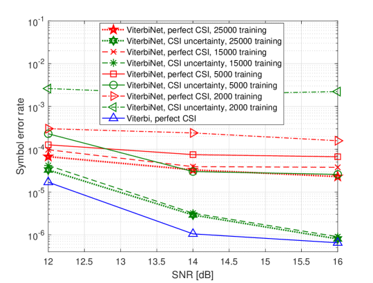
Figure 8: High-SNR performance for different training sizes, ISI channel with AWGN.

The main benefit of ViterbiNet is its ability to accurately implement the Viterbi algorithm in causal finite-memory channels while requiring only knowledge of the memory length, i.e., no CSI is required. The simulation study presented in Figs. 6-7 demonstrates an additional gain of ViterbiNet over the Viterbi algorithm, which is its improved resiliency to inaccurate CSI. Another benefit of ViterbiNet is its ability to reliably operate in setups where, even when full instantaneous CSI is available, the Viterbi algorithm is extremely complicated to implement. To demonstrate this benefit, we again consider the ISI channel in (7) with an exponential decay parameter $\gamma=0.2$, however, here we set the distribution of the additive noise signal $W[i]$ to an alpha-stable distribution [44, Ch. 1]. Alpha-stable distributions, which are obtained as a sum of heavy tailed independent RVs via the generalized central limit theorem, are used to model the noise in various communications scenarios, including molecular channels [45], underwater acoustic channels [46], and impulsive noise channels [47]. In particular, we simulate an alpha-stable noise with stability parameter $\alpha=0.5$, skewness parameter $\beta=0.75$, scale parameter $c=1$, and location parameter $\mu=0$, following [45, Ch. III]. Recall that the PDF of alpha-stable RVs is in general not analytically expressible [44, Ch. 1.4]. Thus, implementing the Viterbi algorithm for such channels is extremely difficult even when full CSI is available, as it requires accurate numerical approximations of the conditional PDFs to compute the log likelihoods. Consequently, in order to implement the Viterbi algorithm here, we numerically approximated the PDF of such alpha-stable RVs using the direct integration method [44, Ch. 3.3] over a grid of $50$ equally spaced points in the range $[-5,5]$, and used the PDF of the closest grid point when computing the log-likelihood terms in the Viterbi detector. In Fig. 9 we depict the SER performance of ViterbiNet compared to the SBRNN detector and the Viterbi algorithm for this channel versus $\rho\in[10,30]$ dB. Observing Fig. 9, we note that the CSI-based Viterbi detector, which has to use a numerical approximation of the PDF, is notably outperformed by the data-driven symbol detectors, which are ignorant of the exact statistical model and do not require an analytical expression of the conditional PDF to operate. Furthermore, we note that ViterbiNet achieves a substantial SNR gap from the SBRNN detector. For example, ViterbiNet achieves an SER smaller than $5\cdot 10^{-2}$ for SNR values larger than $22$ dB, while the SBRNN detector requires an SNR of at least $30$ dB to achieve a similar SER, namely, an SNR gap of $8$ dB. Finally, the performance of ViterbiNet scales with respect to SNR in a similar manner as in Figs. 6-7. The results in Fig. 9 demonstrate the ability of ViterbiNet to reliably operate under non-conventional channel models for which the Viterbi algorithm is difficult to accurately implement, even when full CSI is available.

Figure 9: SER versus SNR, ISI channel with alpha-stable noise.

Finally, we study the robustness of ViterbiNet to different noise powers than those used during training. Recall that so far we have trained ViterbiNet for each value of $\rho$, i.e., for each SNR. To evaluate its resiliency to an inaccurate noise level in training, we next numerically compute the SER of ViterbiNet for different values of the SNR parameter $\rho$. In particular, we repeat the simulation study of the ISI channel with AWGN, whose results are depicted in Fig. 6, while training ViterbiNet using $5000$ samples drawn from a channel with a single SNR, i.e., ViterbiNet is trained once instead of being re-trained for each SNR. The numerically computed SER values are depicted in Fig. 10, where the curves denoted ’ViterbiNet, single SNR’ represent the performance achieved when training only with samples corresponding to a single SNR, which is in the set $\{-2,4,8\}$ dB; The curves denoted ’ViterbiNet, each SNR’ stand for the performance achieved when ViterbiNet is trained anew for each SNR level, i.e., the same curves as those of Fig. 6 of the revised manuscript. Observing Fig. 10, we note that ViterbiNet achieves approximately the same performance when trained using a single SNR value of either $4$ dB or $8$ dB as when it is trained anew for each SNR. A small gap is observed when ViterbiNet is trained using samples corresponding to a low SNR level of $-2$ dB. These results demonstrate the ability of ViterbiNet to generalize to multiple SNR levels.

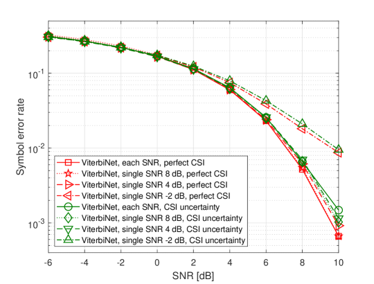
Figure 10: Training for each SNR compared to training over a single SNR, ISI channel with AWGN.

V-B Block-Fading Channels

Next, we numerically evaluate the online training method for tracking block-fading channels detailed in Section IV. To that aim, we consider two block-fading channels: an ISI channel with AWGN and a Poisson channel. For each transmitted block we use the channel models in (7) and (8), respectively, with a fixed exponential decay parameter $\gamma=0.2$, and thus we omit the notation $\gamma$ from the vector ${\boldsymbol{h}}$ in this subsection. However, unlike the scenario studied in the previous subsection, here the channel coefficient vector ${\boldsymbol{h}}$ varies between blocks. In particular, for the $j$th block we use $\big{(}{\boldsymbol{h}}_{(j)}\big{)}_{\tau}\triangleq e^{-0.2(\tau-1)}\cdot\Big{(}0.8+0.2\cos\big{(}\frac{2\pi\cdot j}{\left({\boldsymbol{p}}\right)_{\tau}}\big{)}\Big{)}$, with ${\boldsymbol{p}}=[51,39,33,21]^{T}$. An illustration of the variations in the channel coefficients with respect to the block index $j$ is depicted in Fig. 11.

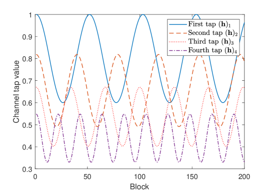
Figure 11: Channel coefficient variations between different blocks.

In each channel block a single codeword of an RS [255, 223] FEC code is transmitted, namely, during each block $b=1784$ bits are conveyed using $t=2040$ binary symbols. Before the first block is transmitted, ViterbiNet is trained using $5000$ training samples taken using the initial channel coefficients, i.e., using the initial channel coefficients vector ${\boldsymbol{h}}_{(1)}$. For online training, we use a learning rate of $0.002$, i.e., five times smaller than that used for initial training, and a bit error threshold of $\bar{\epsilon}=2\%$. In addition to ViterbiNet with online training, we also compute the coded bit error rate (BER) performance of ViterbiNet when trained only once using the $5000$ training samples representing the initial channel ${\boldsymbol{h}}_{(1)}$, referred to as initial training, as well as ViterbiNet trained once using $5000$ training samples corresponding to $10$ different channels $\{{\boldsymbol{h}}_{(3\cdot k)}\}_{k=1}^{10}$, referred to as composite training. The performance of ViterbiNet is compared to the Viterbi algorithm with full instantaneous CSI as well as to the Viterbi detector which assumes that the channel is the time-invariant initial channel ${\boldsymbol{h}}_{(1)}$. The coded BER results, averaged over $200$ consecutive blocks, are depicted in Figs. 12-13 for the ISI channel with AWGN and for the Poisson channel, respectively.

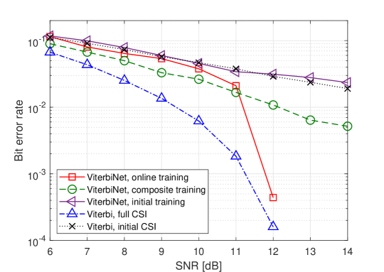
Figure 12: Coded BER versus SNR, block-fading ISI channel with AWGN.

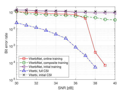
Figure 13: Coded BER versus SNR, block-fading Poisson channel.

Observing Figs. 12-13, we note that for both channels, as the SNR increases, ViterbiNet with online training approaches the performance of the CSI-based Viterbi algorithm which requires accurate knowledge of the complete input-output statistical relationship for each block, while for low SNRs, its performance is only slightly improved compared to that of the Viterbi algorithm using only the initial channel. This can be explained by noting that for high SNR values, the BER at each block is smaller than the threshold $\bar{\epsilon}$, and thus our proposed online training scheme is capable of generating reliable meta-training, which ViterbiNet uses to accurately track the channel, thus approaching the optimal performance. However, for low SNR values, the BER is typically larger than $\bar{\epsilon}$, thus ViterbiNet does not frequently update its coefficients in real-time, thus achieving only a minor improvement over using only the initial training data set. It is emphasized that increasing the BER threshold $\bar{\epsilon}$ can severely deteriorate the performance of ViterbiNet at low SNRs, as it may be trained online using inaccurate meta-training.

We also observe in Figs. 12-13 that the performance ViterbiNet with initial training coincides with that of Viterbi algorithm using the initial channel, as both detectors effectively implement the same detection rule, which is learned by ViterbiNet from the initial channel training set. Furthermore, the composite training approach allows ViterbiNet to achieve improved BER performance compared to using only initial training, as the resulting decoder is capable of operating in a broader range of different channel conditions. Still, is is noted that for both the AWGN channel and the Poisson channel, ViterbiNet with composite training is notably outperformed by the optimal Viterbi detector with instantaneous CSI, whose BER performance is approached only when using online training at high SNRs.

As discussed in Subsection IV-B, the success of the meta-learning based method for training ViterbiNet online depends on the error threshold $\bar{\epsilon}$ and the learning rate used for re-training the DNN. To numerically evaluate the effect of these parameters, we compare in Fig. 14 the BER of ViterbiNet versus $\bar{\epsilon}$ for the ISI with AWGN channel under SNR values of $8$ and $12$ dB, and with re-training learning rates of $0.002$ and $0.02$. These BER values are compared to the model-based Viterbi operating with full CSI. Observing Fig. 14 we note that, for the lower SNR of $8$ dB, a similar behavior, in which the BER value increases with $\bar{\epsilon}$, is observed for both learning rates. However, for the higher SNR of $12$ dB, the BER increase with the error threshold $\bar{\epsilon}$ for learning rate of $0.002$, while for the higher learning rate of $0.02$ we observe a minima around $\bar{\epsilon}=0.04$. This behavior is because higher values of $\bar{\epsilon}$ may cause the network to use inaccurate training, while values which are too small may result in the network being unable to reliably track channel variations.

Figure 14: Coded BER versus error threshold, block-fading ISI channel with AWGN.

The results presented in this section demonstrate that a data-driven symbol detector designed by integrating DNNs into the Viterbi algorithm is capable of approaching optimal performance without CSI. Unlike the CSI-based Viterbi algorithm, its ML-based implementation demonstrates robustness to imperfect CSI, and achieves excellent performance in channels where the Viterbi algorithm is difficult to implement. The fact that ViterbiNet requires a relatively small training set allows it to accurately track block-fading channels using meta-training generated from previous decisions on each transmission block. We thus conclude that designing a data-driven symbol detector by combining ML-based methods with the optimal model-based algorithm yields a reliable, efficient, and resilient data-driven symbol recovery mechanism.

VI Conclusions

We proposed an ML-based implementation of the Viterbi symbol detection algorithm called ViterbiNet. To design ViterbiNet, we identified the log-likelihood computation as the part of the Viterbi algorithm that requires full knowledge of the underlying channel input-output statistical relationship. We then integrated an ML-based architecture designed to compute the log-likelihoods into the algorithm. The resulting architecture combines ML-based processing with the conventional Viterbi symbol detection scheme. In addition, we proposed a meta-learning based method that allows ViterbiNet to track time-varying channels online. Our numerical results demonstrate that ViterbiNet approaches the optimal performance of the CSI-based Viterbi algorithm and outperforms previously proposed ML-based symbol detectors using a small amount of training data. It is also illustrated that ViterbiNet is capable of reliably operating in the presence of CSI uncertainty, as well as in complex channel models where the Viterbi algorithm is extremely difficult to implement. Finally, it is shown that ViterbiNet can adapt via meta-learning in block-fading channel conditions.

References

- [1] A. Viterbi. “Error bounds for convolutional codes and an asymptotically optimum decoding algorithm”. IEEE Trans. Inform. Theory, vol. 13, no. 2, Apr. 1967, pp. 260–269.
- [2] G. D. Forney. “The Viterbi algorithm”. Proc. IEEE, vol. 61, no. 3, Mar. 1973, pp. 268–278.
- [3] Y. LeCun, Y. Bengio, and G. Hinton. “Deep learning”. Nature, vol. 521, no. 7553, May 2015, pp. 436–444.
- [4] Y. Bengio. “Learning deep architectures for AI”. Foundations and Trends in Machine Learning, vol. 2, no. 1, 2009, pp. 1–127.
- [5] K. Gregor and Y. LeCun. “Learning fast approximations of sparse coding”. Proc. ICML, Haifa, Israel, Jun. 2010.
- [6] S. Khobahi, N. Naimipour, M. Soltanalian, and Y. C. Eldar. “Deep signal recovery with one-bit quantization”. Proc. ICASSP, Brighton, UK, May 2019.
- [7] T. O’Shea and J. Hoydis. “An introduction to deep learning for the physical layer”. IEEE Trans. on Cogn. Commun. Netw., vol. 3, no. 4, Dec. 2017, pp. 563–575.
- [8] O. Simeone. “A very brief introduction to machine learning with applications to communication systems”. IEEE Trans. on Cogn. Commun. Netw., vol. 4, no. 4, Dec. 2018, pp. 648–664.
- [9] Q. Mao, F. Hu and Q. Hao. “Deep learning for intelligent wireless networks: A comprehensive survey”. IEEE Commun. Surveys Tuts., vol. 20, no. 4, 2018, pp. 2595–2621.
- [10] D. Gunduz, P. de Kerret, N. D. Sidiropoulos, D. Gesbert, C. Murthy, and M. van der Schaar. “Machine learning in the air”. arXiv preprint, arXiv:1904.12385, 2019.
- [11] E. Nachmani, E. Marciano, L. Lugosch, W. J. Gross, D. Burshtein, and Y. Be’ery. “Deep learning methods for improved decoding of linear codes”. IEEE J. Sel. Topics Signal Process., vol 12, no. 1, Feb. 2018, pp. 119–131.
- [12] T. Gruber, S. Cammerer, J. Hoydis, and S. ten Brink. “On deep learning based channel decoding”. Proc. CISS, Baltimore, MD, Mar. 2017.
- [13] N. Samuel, T. Diskin and A. Wiesel. “Deep MIMO detection”. Proc. SPAWC, Sapporo, Japan, Jul. 2017.
- [14] A. Caciularu and D. Burshtein. “Blind channel equalization using variational autoencoders”. arXiv preprint, arXiv:1803.01526, 2018.
- [15] N. Farsad and A. Goldsmith. “Neural network detection of data sequences in communication systems”. IEEE Trans. Signal Process., vol. 66, no. 21, Nov. 2018, pp. 5663–5678.
- [16] F. Liang, C. Shen, and F. Wu. “An iterative BP-CNN architecture for channel decoding”. IEEE J. Sel. Topics Signal Process., vol 12, no. 1, Feb. 2018, pp. 144–159.
- [17] H. Kim, Y. Jiang, R. Rana, S. Kannan, S. Oh, and P. Viswanath. “Communication Algorithms via deep learning”. arXiv preprint, arXiv:1805.09317, 2018.
- [18] X. A. Wang and S. B. Wicker. “An artificial neural net Viterbi decoder”. IEEE Trans. Commun., vol. 44, no. 2, Feb. 1996, pp. 165–171.
- [19] M. Shohat, G. Tsintsadze. N. Shlezinger, and Y. C. Eldar. “Deep quantization for MIMO channel estimation”. Proc. ICASSP, Brighton, UK, May 2019.
- [20] J. R. Hershey, J. Le Roux, and F. Weninger. “Deep unfolding: Model-based inspiration of novel deep architectures”. arXiv preprint, arXiv:1409.2574, 2014.
- [21] P. Sprechmann, A. M. Bronstein, and G. Sapiro. “Supervised non-euclidean sparse NMF via bilevel optimization with applications to speech enhancement”. Proc. HSCMA, Villers-les-Nancy, France, May. 2014.
- [22] Y. Li, M. Tofighi, J. Geng, V. Monga and Y. C. Eldar. “An algorithm unrolling approach to deep blind image deblurring”. arXiv preprint, arXiv:1902.03493, 2019.
- [23] O. Solomon, R. Cohen, Y. Zhang, Y, Yang, H. Qiong, J. Luo, R. J.G. van Sloun, and Y. C. Eldar. “Deep unfolded robust PCA with application to clutter suppression in ultrasound”. arXiv preprint, arXiv:1811.08252, 2018.
- [24] C. Lemke, M. Budka, and B. Gabrys. “Metalearning: A survey of trends and technologies”. AI Rev., vol 44, no. 1, Jun. 2015, pp. 117–130.
- [25] S. Park, H. Jang, O. Simeone, and J. Kang. “Learning how to demodulate from few pilots via meta-learning”. arXiv preprint, arXiv:1903.02184, 2019.
- [26] D. Tse and P. Viswanath. Fundamentals of Wireless Communication. Cambridge, 2005.
- [27] D. D. Falconer and F. R. Magee. “Adaptive channel memory truncation for maximum likelihood sequence estimation”. Bell System Technical Journal, vol. 52, no. 9, Nov. 1973, pp. 1541–1562.
- [28] V. D. Nguyen, H-P. Kuchenbecker, H. Haas, K. Kyamakya, and G. Gelle. “Channel impulse response length and noise variance estimation for OFDM systems with adaptive guard interval”. J. Wireless Com. Network., Dec. 2007.
- [29] A. van den Oord, S. Dieleman, H. Zen, K. Simonyan, O. Vinyals, A. Graves, N. Kalchbrenner, A. Senior, and K. Kavukcuoglu. “WaveNet: A generative model for raw audio”. arXiv preprint, arXiv:1609.03499, 2016.
- [30] A. van den Oord, N. Kalchbrenner, L. Espeholt, O. Vinyals, and A. Graves. “Conditional image generation with PixelCNN decoders”. Proc. NIPS, 2016, pp. 4790-4798.
- [31] M. Rosenblatt. “Remarks on some nonparametric estimates of a density function”. The Annals of Mathematical Statistics, vol 27, no. 3, Sep. 1956, pp. 832–837.
- [32] G. McLachlan and D. Peel. Finite Mixture Models. Wiley Press, 2004.
- [33] E. Dahlman, S. Parkvall, J. Skold, and P. Beming. 3G Evolution: HSPA and LTE for Mobile Broadband. Academic Press, 2010.
- [34] C. Bishop. “Mixture density networks”. Technical Report, Aston University, UK, 1994.
- [35] N. Shlezinger, R. Fu, and Y. C. Eldar. “DeepSIC: Deep soft interference cancellation for multiuser MIMO detection”. Submitted to the IEEE J. Sel. A. Inform. Theory, 2019.
- [36] W. J. Choi, K. W. Cheong, and J. M. Cioffi. “Iterative soft interference cancellation for multiple antenna systems”. Proc. WCNC, Chicago, IL, Sep. 2000.
- [37] L. Bahl, J. Cocke, F. Jelinek, and J. Raviv. “Optimal decoding of linear codes for minimizing symbol error rate”. IEEE Trans. Inform. Theory, vol. 20, no. 2, Mar. 1974, pp. 284–287.
- [38] X. Lingyun and D. Limin. “Efficient Viterbi beam search algorithm using dynamic pruning”. Proc. ICSP, Beijing, China, Aug. 2004.
- [39] W. H. Gerstacker and R. Schober. “Equalization concepts for EDGE”. IEEE Trans. Wireless Commun., vol. 1, no. 1, Jan. 2002, pp. 190–199.
- [40] B. Hassibi and B. M. Hochwald. “How much training is needed in multiple-antenna wireless links?”. IEEE Trans. Inform. Theory, vol. 49, no. 4, Apr. 2003, pp. 951–963.
- [41] N. Shlezinger and R. Dabora. “Frequency-shift filtering for OFDM signal recovery in narrowband power line communications,” IEEE Trans. Commun., vol. 62, no. 4, Apr. 2014, pp. 1283-1295.
- [42] A. J. Goldsmith. Wireless Communications. Cambridge, 2005.
- [43] D. P. Kingma and J. L. Ba. “Adam: A method for stochastic optimization”. arXiv preprint, arXiv:1412.6980v9.
- [44] J. P. Nolan. Stable distributions: Models for heavy-tailed data. Birkhauser, 2003.
- [45] N. Farsad, Y. Murin, W. Guo, C-B. Chae, A. W. Eckford, and A. J. Goldsmith. “Communication system design and analysis for asynchronous molecular timing channels”. IEEE Trans. Mol. Biol. Multi-Scale Commun., vol. 3, no. 4, Dec. 2017, pp. 239–253.
- [46] K. Pelekanakis and M. Chitre. “Robust equalization of mobile underwater acoustic channels”. IEEE J. Ocean. Eng., vol. 40, no. 4, Oct. 2015, pp. 775–784.
- [47] Z. Mei, M. Johnston, S. Le Goff, and L. Chen. “Performance analysis of LDPC-coded diversity combining on Rayleigh fading channels with impulsive noise”. IEEE Trans. Commun., vol. 65, no. 6, Jun. 2017, pp. 2345–2356.