Complexity of Hyperscaling Violating Theories at Finite Cutoff

Mohsen Alishahiha^& and Amin Faraji Astaneh^†,∗

^& School of Physics, Institute for Research in Fundamental Sciences (IPM)
P.O. Box 19395-5531, Tehran, Iran
^† Physics Department, Faculty of Sciences, Arak University, Arak 38156-8-8349, Iran
^∗ School of Particles and Accelerators,
Institute for Research in Fundamental Sciences (IPM)
P.O. Box 19395-5531, Tehran, Iran

E-mails: alishah@ipm.ir, faraji@ipm.ir

Using the complexity equals action proposal we study holographic complexity for hyperscaling violating theories in the presence of a finite cutoff that, in turns, requires to obtain all counter terms needed to have finite boundary energy momentum tensor. These terms could give non-trivial contributions to the complexity. We observe that having a finite UV cutoff would enforce us to have a cutoff behind the horizon of which the value is fixed by the UV cutoff; moreover, certain counter term should be defined on the cutoff behind the horizon too.

1 Introduction

In the context of AdS/CFT correspondence [1] it was proposed that $T\bar{T}$ deformation of a two dimensional conformal field theory [2] has an interesting holographic dual in terms of an AdS₃ geometry with a finite radial cutoff[3], see also [4]. Generalization of $T\bar{T}$ deformation to higher dimensional conformal field theories has also been studied in [5, 6] where it was proposed that the corresponding deformation has a gravitational dual given by a higher dimensional AdS (black brane) geometry with a finite radial cutoff.

Using gravitational description of $T\bar{T}$ deformation of a conformal field theory, the holographic complexity for the black brane solutions of the Einstein gravity at a finite radial cutoff was studied in [7] where it was shown that the finite UV cutoff induces a cutoff behind the horizon (see also [8, 9]). In particular it was shown that the presence of the behind the horizon cutoff is crucial to find the expected result for the holographic complexity of the Jackiw-Teitelboim gravity [10]. It is also important to note that in order to get the desired result one needs to consider contributions of certain counter terms appearing in the context of holographic renormalization that are usually required to get finite on shell action.

As motivated above, in order to further illustrate the roles of the counter terms and the behind the horizon cutoff, in this paper we will study holographic complexity for theories with hyperscaling violation at a finite cutoff. We note that complexity for hyperscaling violating theories has been already studied in [13, 14]. Of course in what follows the aim is to explore the effect of a finite UV cutoff in the computations of complexity. Indeed, we will see that in this case in order to get a consistent result for the complexity one is forced to have a cutoff behind the horizon of which the value is fixed by the finite UV cutoff. We note also that besides this cutoff there are certain counter terms whose contributions should be taken into account too.

To proceed, first of all, one needs to study the hyperscaling violating geometry in the presence of a finite radial cutoff which might be thought of as a $T\bar{T}$-like generalization of non-relativistic theories. Actually to read the energy of the system with a UV cutoff one needs to fully study all possible counter terms required to get finite boundary energy momentum tensor. Indeed, this is what we will do in the present paper by which we will be able to compute the finite cutoff corrections to the energy.

Geometries with hyperscaling violating factor have been studied in [15, 16]. To fix our notation, as a minimal model, we will consider an Einstein-Dilaton-Maxwell theory in $d+2$ dimensions whose action may be given by [17]

$$S^{\rm bulk}\!\! \!\!=\!\! \!\!\frac{1}{16\pi G}\int d^{d+2}x\sqrt{-g}\left[R-\frac{1}{2}(\partial\phi)^{2}+V(\phi)-\frac{1}{4}e^{\eta\phi}F^{2}\right],$$ (1.1)

$$S^{\rm GH}\!\! \!\!=\!\! \!\!\frac{1}{8\pi G}\int d^{d+1}x\sqrt{-h}K.$$ (1.3)

The Gibbons-Hawking action is required to have a well defined variational principle. Nonetheless its presence is curtail for other purposes such as to find finite free energy. It may also have non-trivial contribution to the holographic complexity. As for a potential we will consider the following term

$$V=V_{0}e^{\zeta\phi}.$$ (1.4)

Here $\eta,\zeta$ and $V_{0}$ are free parameters of the model. This model, indeed, admits solutions with hyperscaling violation and non-trivial anisotropy. In fact, the vector field is required to produce an anisotropy while non-trivial potential, as given above, is needed to have hyperscaling violating factor. The corresponding black brane solution is

$$ds^{2}\!\! \!\!=\!\! \!\!r^{-2{\theta}_{e}}\left(-r^{2z}f(r)dt^{2}+\frac{dr^{2}}{r^{2}f(r)}+r^{2}d\vec{x}^{2}\right),\;\;\;\;\;\;\;\;\;\;\;f(r)=1-\frac{r_{h}^{z+d_{e}}}{r^{z+d_{e}}}\,,$$ (1.5)

$$A_{t}(r)\!\! \!\!=\!\! \!\!\sqrt{\frac{2(z-1)}{z+d_{e}}}\;r^{z+d_{e}}f(r),\;\;\;\;\;\;\;\;\;\;\;\;\;\;\;\;\;\;\;\;\;\;\;\;\;\;\;\;\;\;\;\;\;\;\;\;\;\;\;\;\;e^{\eta\phi}=r^{-2(d_{e}+{\theta}_{e})}\,,$$ (1.7)

where $r_{h}$ is the radius of horizon. Note that in our notations the boundary is located at $r_{\infty}\rightarrow\infty$. Here $\theta_{e}=\frac{\theta}{d}$ and $d_{e}=d-\theta$ may be thought of as effective hyperscaling and dimension, respectively. $z$ is also the anisotropy exponent. The parameters of the solution and those of the action are related by

$$\eta=\frac{-2(d_{e}+{\theta}_{e})}{\sqrt{2d_{e}(z-1-{\theta}_{e})}},\;\;\;\;\;\;\;\;V_{0}=(z+d_{e}-1)(z+d_{e}),\;\;\;\;\;\;\;\;\zeta=\frac{{2\theta}_{e}}{\sqrt{2d_{e}(z-1-{\theta}_{e})}}\,.$$ (1.8)

Note that there is no charge associated with the gauge field, even though there is a non-zero gauge field. Indeed, its effect is just to reproduce an anisotropy and thus setting $z=1$ the gauge field vanishes. This geometry provides a holographic description of a field theory with hyperscaling violating symmetry in $d+1$ dimensions.

The rest of the paper is organized as follows. In the following section we will study holographic energy at the finite cutoff. To do so, one will have to find certain counter terms required to get finite on shell action when evaluated over the whole space time. These counter terms are also needed to have finite energy momentum tensor. In section four using “complexity equals action” proposal we will compute complexity of hyperscaling violating theories with a finite cutoff. We shall see that to find a consistent result a cutoff behind the horizon is required whose value is given by the finite cutoff. It is also important to have certain boundary terms that contribute to the complexity. The last section is devoted to discussions where we will also give a comment on a possible holographic dual description of a $T\bar{T}$-like deformation of a theory with hyperscaling violation.

2 Holographic energy at a finite cutoff

In this section we will compute the energy of the model when there is a finite radial cutoff. To do so, one needs regularized boundary energy momentum tensor that, in turn, requires to have full action including all counter terms to make the gravitational free energy finite.

Therefore in what follows we will first compute free energy of the solution (1.5). To proceed we note that for the solution (1.5) one has

$$\sqrt{-g}\left(R-\frac{1}{2}(\partial\phi)^{2}+V_{0}e^{\xi\phi}-\frac{1}{4}e^{\eta\phi}F^{2}\right)=-2(1-{\theta}_{e})(d_{e}+z){r^{d_{e}+z-1}},$$ (2.1)

leading to the following expression for the bulk part of the action

$$S^{\rm bulk}=-\frac{V_{d+1}(1-\theta_{e})(z+d_{e})}{8\pi G_{N}d}\int_{r_{h}}^{r_{\infty}}dr\,r^{z+d_{e}-1}=(1-{\theta}_{e})\frac{V_{d+1}}{8\pi G_{N}}\left(-r_{\infty}^{z+d_{e}}+r_{h}^{z+d_{e}}\right),$$ (2.2)

where $r_{\infty}$ is a UV cutoff that will eventually be sent to infinity. On the other hand for the Gibbons-Hawking term one finds

$$S^{\rm GH}=(z+d_{e}-{\theta}_{e})\frac{V_{d+1}}{8\pi G_{N}}r_{\infty}^{z+d_{e}}-(z+d_{e}-{2\theta}_{e})\frac{V_{d+1}}{16\pi G_{N}}r_{h}^{z+d_{e}}\,.$$ (2.3)

Putting both contributions together one arrives at

$$S^{\rm bulk}+S^{\rm GH}=(z+d_{e}-1)\frac{V_{d+1}}{8\pi G_{N}}r_{\infty}^{z+d_{e}}-(z+d_{e}-2)\frac{V_{d+1}}{16\pi G_{N}}r_{h}^{z+d_{e}}\,,$$ (2.4)

that is divergent as $r_{\infty}$ approaches infinity. It is, of course, known that to remove all divergent terms one needs to add certain counter terms that play an important role in the context of holographic renormalization [18]. For the cases in which the model has non-zero anisotropy exponent the corresponding counter terms have been studied in [19]. Motivated by this paper and to accommodate non-zero hyperscaling violating factor we will consider the following ansatz for the counter term

$$S^{\rm ct}=-\frac{1}{16\pi G_{N}}\int d^{d+1}x\sqrt{-h}\,e^{\frac{1}{2}\zeta\phi}(c_{1}+c_{2}\,e^{\eta\phi}A_{\mu}A^{\mu})\,$$ (2.5)

where $c_{1}$ and $c_{2}$ are two numerical constants that may be fixed by requiring the finiteness of the free energy that produces desired entropy of the black brane. For the black hole solution (1.5) the above counter term reads

$$S^{\rm ct}=-\frac{V_{d+1}}{16\pi G_{N}}\left(c_{1}-\frac{2c_{2}(z-1)}{d_{e}+z}\right)r_{\infty}^{d_{e}+z}+\frac{V_{d+1}}{32\pi G_{N}}\left(c_{1}-\frac{6c_{2}(z-1)}{d_{e}+z}\right)r_{h}^{z+d_{e}}.$$ (2.6)

It is then easy to see that requiring to have finite free energy that gives correct entropy one should have

$$c_{1}=2d_{e}+z-1,\;\;\;\;\;\;\;\;\;\;\;c_{2}=-\frac{z+d_{e}}{2}\,,$$ (2.7)

so that

$$S^{\rm tot}=S^{\rm bulk}+S^{\rm GH}+S^{\rm ct}=\frac{zV_{d+1}}{16\pi G_{N}}r_{h}^{z+d_{e}}\,.$$ (2.8)

The next step is to check whether the above counter term is enough to have finite (regular) boundary energy momentum tensor. To see this, one needs to compute the corresponding boundary energy momentum tensor for our model. Following [19] one should note that there are several parts that contribute to the boundary energy momentum tensor which may be decomposed as follows

$$T^{\mu}_{\nu}=T^{({\rm b})\mu}_{\nu}+T^{({\rm c})\mu}_{\nu}+\tau^{({\rm b})\mu}_{\nu}+\tau^{({\rm c})\mu}_{\nu}\,,$$ (2.9)

where $(b)$ and $(c)$ stand for “bulk” and “counter term” that indicate whether the corresponding term comes from bulk action (including Gibbons-Hawking term) or the counter term. More explicitly one has

$$\!\!T^{({\rm b})\mu}_{\nu}=\frac{1}{8\pi G_{N}}(K^{\mu}_{\nu}-\delta^{\mu}_{\nu}K)\ ,\,\;\;\;T^{({\rm c})\mu}_{\nu}=\frac{2d_{e}+z-1}{16\pi G_{N}}e^{\frac{1}{2}\zeta\phi}\,\delta^{\mu}_{\nu}+\frac{z+d_{e}}{16\pi G_{N}}e^{\eta\phi+\frac{1}{2}\zeta\phi}(A^{\mu}A_{\nu}-\frac{1}{2}\delta^{\mu}_{\nu}A_{\alpha}A^{\alpha})\,,$$

$$\!\!\tau^{({\rm b})\mu}_{\nu}=\frac{1}{16\pi G_{N}}e^{\eta\phi}n_{\alpha}F^{\alpha\mu}A_{\nu}\,,\;\;\;\;\;\;\;\tau^{({\rm c})\mu}_{\nu}=-\frac{z+d_{e}}{16\pi G_{N}}e^{\eta\phi+\frac{1}{2}\zeta\phi}A^{\mu}A_{\nu}\,.$$ (2.10)

In fact, the the first term is the standard Brown-York energy momentum tensor. It is worth noting that for the model we are considering the energy momentum tensor is not symmetric [19]. By making use of the explicit form of the black brane solution (1.5) different components of the energy momentum tensor read

$$\!\!T^{(\rm b)t}_{t}=-\frac{d_{e}}{8\pi G_{N}}f^{\frac{1}{2}}r^{{\theta}_{e}}\ ,\,\;\;\;\;\;\;\;\;\;\;\;\;\;\;\;\;\;\;\;\;\;\;\;\;\;\;\;T^{(\rm b)i}_{j}=\frac{-1}{16\pi G_{N}}f^{-\frac{1}{2}}[z+d_{e}+(z+d_{e}-2)f]\,r^{{\theta}_{e}}\delta^{i}_{j}\,,$$

$$\!\!T^{(\rm c)t}_{t}=\frac{1}{16\pi G_{N}}[2d_{e}+z-1-(z-1)f]\,r^{{\theta}_{e}}\,,\;\;\;T^{(\rm c)i}_{j}=\frac{1}{16\pi G_{N}}[2d_{e}+z-1+(z-1)f]r^{{\theta}_{e}}\delta^{i}_{j}\,,$$

$$\!\!\tau^{(\rm b)t}_{t}=-\frac{z-1}{8\pi G_{N}}f^{1/2}r^{{\theta}_{e}}\,,\;\;\;\;\;\;\;\;\;\;\;\;\;\;\;\;\;\;\;\;\;\;\;\tau^{(\rm c)t}_{t}=\frac{z-1}{8\pi G_{N}}f\,r^{{\theta}_{e}}\,.$$ (2.11)

Utilizing the holographic renormalization procedure [18] one may define the expectation value of different components of the dual field theory energy moment as follows

$$\hat{T}^{\mu}_{\nu}=\lim_{r_{\infty}\rightarrow\infty}r_{\infty}^{z+d_{e}-{\theta}_{e}}\ T^{\mu}_{\nu}\,,$$ (2.12)

that more explicitly are given by

$$\!\!\hat{T}^{(\rm b)t}_{t}=\frac{-1}{8\pi G_{N}}(d_{e}\,r_{\infty}^{z+d_{e}}-\frac{d_{e}}{2}r_{h}^{z+d_{e}})\,,\;\;\;\hat{T}^{(\rm c)t}_{t}=\frac{1}{8\pi G_{N}}(d_{e}\,r_{\infty}^{z+d_{e}}+\frac{z-1}{2}r_{h}^{z+d_{e}})\,,$$ (2.13)

$$\!\!\hat{\tau}^{({\rm b})t}_{t}=\frac{-1}{8\pi G_{N}}((z-1)r_{\infty}^{z+d_{e}}-\frac{z-1}{2}r_{h}^{z+d_{e}})\,,\;\;\;\hat{\tau}^{({\rm c})t}_{t}=\frac{1}{8\pi G_{N}}((z-1)r_{\infty}^{z+d_{e}}-(z-1)r_{h}^{z+d_{e}})\,,$$

$$\!\!\hat{T}^{({\rm b})i}_{j}=\frac{-1}{8\pi G_{N}}((z+d_{e}-1)r_{\infty}^{z+d_{e}}+\frac{1}{2}r_{h}^{z+d_{e}})\delta^{i}_{j}\,,\;\;\;\hat{T}^{({\rm c})i}_{j}=\frac{1}{8\pi G_{N}}((z+d_{e}-1)r_{\infty}^{z+d_{e}}-\frac{z-1}{2}r_{h}^{z+d_{e}})\delta^{i}_{j}\,.$$

It is then easy to sum up the corresponding terms resulting in

$$\hat{T}^{t}_{t}=\frac{d_{e}}{16\pi G_{N}}r_{h}^{z+d_{e}}\ \ ,\ \ \hat{T}^{i}_{j}=\frac{-z}{16\pi G_{N}}\delta^{i}_{j}r_{h}^{z+d_{e}}\,,$$ (2.14)

which can be used to find the trace condition for the theory as follows

$$z\,\hat{T}^{t}_{t}+\frac{d_{e}}{d}\,\hat{T}^{i}_{i}=0\,.$$ (2.15)

Therefore, the counter term we have considered is also enough to have finite energy momentum tensor. The same argument can be deduced for the expectation value of the operator dual to the dilaton field. It is then straightforward to compute the energy of the solution with or without cutoff. In particular setting the theory at a radial cutoff $r=r_{c}$ the corresponding energy is found

$${E}\!\! \!\!=\!\! \!\!r_{c}^{z-{\theta}_{e}}\int d^{d}x\sqrt{g}\ T^{t}_{t}=\frac{V_{d}}{16\pi G_{N}}r_{c}^{z+d_{e}}\left(\sqrt{f(r_{c})}-1\right)\left(-2d_{e}+(z-1)(\sqrt{f(r_{c})}-1\right)$$ (2.16)

$$\!\!=\!\! \!\!\frac{(z+d_{e}-1)V_{d}}{8\pi G_{N}}r_{c}^{z+d_{e}}\left(1-\sqrt{1-\frac{r_{h}^{z+d_{e}}}{r_{c}^{z+d_{e}}}}\right)-\frac{(z-1)V_{d}}{16\pi G_{N}}r_{h}^{z+d_{e}},$$ (2.18)

which may be recast into the following form

$${E}=\frac{d_{e}V_{d}}{16\pi G_{N}}r_{h}^{z+d_{e}}+\frac{(d_{e}+z-1)V_{d}}{16\pi G_{N}}r_{c}^{z+d_{e}}\left(1-\sqrt{1-\frac{r_{h}^{z+d_{e}}}{r_{c}^{z+d_{e}}}}\right)^{2}\,.$$ (2.19)

This is indeed the final form of the energy at a finite cutoff that will be used when we want to study the late time behavior of the complexity. The same behavior of the energy can be seen in [20] where the $T\bar{T}$ deformation of a two dimensional Lifshitz theory has been studied.

It is worth noting that in the large cutoff limit, $r_{c}\rightarrow\infty$, the second term in the above expression vanishes leaving us with the first term that is, indeed, the mass of the black hole solution (1.5).

3 Complexity at finite cutoff

In this section we would like to compute the holographic complexity for the hyperscaling violating geometry with a finite cutoff denoted by $r_{c}$ as shown in the figure 1.

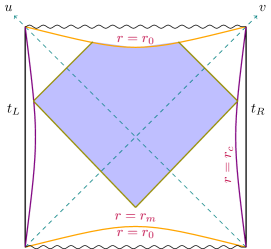
Figure 1: The WDW patch for the theory at finite cutoff $r_{c}$. There is also a cutoff behind the horizon, $r_{0}$ of which the value is fixed by UV cutoff $r_{c}$.

The holographic complexity for such geometries have been studied in [13, 14] where it was shown that at the late time the complexity growth approaches the following constant

$$\frac{d{\cal C}}{d\tau}=\frac{d_{e}+z-1}{d_{e}}\,2E_{0},$$ (3.1)

where $E_{0}$, the energy of the back brane, is given by

$$E_{0}=\frac{d_{e}V_{d}}{16\pi G_{N}}r_{h}^{d+z}.$$ (3.2)

Although it violates the naive Lloyd’s bound given by the twice of the energy [21], it is still given by a constant related to the energy of the system. Having put the system at a finite cutoff one would expect that the late time behavior of complexity should be given in terms of the deformed energy (2.19) as follows

$$\frac{d{\cal C}}{d\tau}=\frac{d_{e}+z-1}{d_{e}}\,2E.$$ (3.3)

This is what we would like to explore in this section using “complexity=action” proposal (CA) for the holographic complexity. According to this proposal the quantum computational complexity of a holographic state is given by the on-shell action evaluated on a bulk region known as the “Wheeler-De Witt” (WDW) patch [22, 23]

$${\cal C}(\Sigma)=\frac{I_{\rm WDW}}{\pi\hbar}.$$ (3.4)

Here the WDW patch is defined as the domain of dependence of any Cauchy surface in the bulk whose intersection with the asymptotic boundary is the time slice $\Sigma$.

Based on the CA proposal, we evaluate the on shell action of the WDW patch shown in the figure 1 where the WDW patch is restricted by the UV cutoff $r_{c}$. For further use we have also set another cutoff near singularity at $r=r_{0}$. In principle, one might naively expect that the cutoff $r_{0}$ can be sent to zero at the end of the day. As we will see this is not the case and indeed our ultimate goal is to explore the role of this cutoff.

It is worth mentioning that the on shell action evaluated on a WDW patch gets different contributions from different parts of the action including bulk, boundary and corner parts [24, 25, 26, 27]. In what follows we will compute each conurbation when the corresponding WDW patch is bounded by two cutoffs: $r_{c}$ and $r_{0}$.

To proceed let us fix our notations for the boundary and the joint points at first. Two null boundaries of the corresponding WDW patch terminating to the joint point $r_{m}$ are given by

$$t=t_{R}-r^{*}(r_{c})+r^{*}(r),\;\;\;\;\;\;\;\;\;t=-t_{L}+r^{*}(r_{c})-r^{*}(r),$$ (3.5)

by which the joint point $r_{m}$ is given by $\tau=2(r^{*}(r_{c})-r^{*}(r))$, with $r^{*}(r)=\int\frac{dr}{r^{z+1}f(r)}$. Here $t_{L}(t_{R})$, is time coordinate of left (right) boundary located at the cutoff surface $r=r_{c}$ and, the boundary time is defined by $\tau=t_{L}+t_{R}$. The null vectors associated with these null boundaries are also given by

$$k_{1}=\alpha\left(\partial_{t}+\frac{\partial_{r}}{r^{z+1}f(r)}\right),\;\;\;\;\;\;\;\;\;\;\;\;\;\;\;k_{2}=\beta\left(-\partial_{t}+\frac{\partial_{r}}{r^{z+1}f(r)}\right),$$ (3.6)

where $\alpha$ and $\beta$ are two free parameters appearing due to ambiguity associated to the definition of norms of the null vectors. We note also that in our notation we have a space like boundary at $r=r_{0}$ of which the normal vector is given by $n=\frac{\partial_{r}}{r_{0}^{\theta_{e}+1}\sqrt{|f(r_{0})|}}$.

To compute the on shell action let us start from the bulk part that is essentially given by bulk action given in equation (1.1) evaluated for the solution (1.5). The bulk contribution to the on shell action is

$$S^{\rm bulk}\! \!=\! \!-\frac{V_{d}}{2\pi G_{N}}(1-{\theta}_{e})(d_{e}+z)\int_{r_{0}}^{r_{c}}{dr}\,{r^{d_{e}+z-1}}\left({r^{*}(r_{c})-r^{*}(r)}\right)$$ (3.9)

$$-\frac{V_{d}}{4\pi G_{N}}(1-{\theta}_{e})(d_{e}+z)\int_{r_{0}}^{r_{m}}{dr}\,{r^{d_{e}+z-1}}\left({\frac{\tau}{2}-r^{*}(r_{c})+r^{*}(r)}\right),$$

that might be simplified to find

$$S^{\rm bulk}=\frac{(1-\theta_{e})V_{d}}{4\pi G}\left(\frac{r_{m}^{d_{e}}+r_{0}^{d_{e}}-2r_{c}^{d_{e}}}{d_{e}}+\left(\frac{\tau}{2}+r^{*}(r_{c})-r^{*}(r_{0})\right)r_{0}^{d_{e}+z}f(r_{0})\right)\,.$$ (3.10)

In the next step we consider the contribution of the joint points. In the present case there are five corners two of which at UV cutoff, the other two at the behind the horizon cutoff and the last one at the joint point $r_{m}$. The action of a joint point has the following general form [26]

$$\pm\frac{1}{8\pi G}\int d^{d}x\,d\lambda\sqrt{\gamma}\,\log a$$ (3.11)

where $a$ is the inner product of the normal vectors associated with two corresponding intersecting boundaries (there is also a factor of one-half if both boundaries are null). Here $\gamma$ is determinant of the induced metric on the joint points and $\lambda$ is the null coordinate defined on the null segments that we choose to be Affine. The “$\pm$” sings tell us which corner contribution is being computed (for more details see [26]). In fact using the above normal vectors given in the equation (3.6) one may compute the contribution of corner points

$$S^{\rm joint}\!\! \!\!=\!\! \!\!\frac{V_{d}}{8\pi G}(z-\theta_{e})\left(2r_{c}^{d_{e}}\log r_{c}^{2}-r_{m}^{d_{e}}\log r_{m}^{2}-r_{0}^{d_{e}}\log r_{0}^{2}\right)+\frac{V_{d}}{8\pi G}(r_{m}^{d_{e}}+r_{0}^{d_{e}}-2r_{c}^{d_{e}})\log\alpha\beta$$ (3.12)

$$\!\!+\!\! \!\!\frac{V_{d}}{8\pi G}\left(2r_{c}^{d_{e}}\log|f(r_{c})|-r_{m}^{d_{e}}\log|f(r_{m})|-r_{0}^{d_{e}}\log|f(r_{0})|\right)\,.$$ (3.14)

From the second term it is clear that the on shell action suffers from an ambiguity associated with the definition of null vectors as mentioned above. Indeed, in order to remove this ambiguity one needs to add extra counter terms associated to each null boundaries. The corresponding counter term is [26, 28]

$$\pm\frac{1}{8\pi G}\int d\lambda d^{d}x\sqrt{\gamma}\,\Theta\log\frac{|\Theta|}{d_{e}}$$ (3.15)

which should be evaluated on all null boundaries with a proper sign (see [26] for more details). Here $\Theta$ is defined by

$$\Theta=\frac{1}{\sqrt{\gamma}}\frac{\partial\sqrt{\gamma}}{\partial\lambda},$$ (3.16)

It is then straightforward to compute the contribution of this term for all null boundaries

$$S^{\rm ct}_{1}\!\! \!\!=\!\! \!\!\frac{V_{d}}{4\pi G}\frac{z-2\theta_{e}}{d_{e}}(2r_{c}^{d_{e}}-r_{m}^{d_{e}}-r_{0}^{d_{e}})+\frac{V_{d}}{8\pi G}(2r_{c}^{d_{e}}-r_{m}^{d_{e}}-r_{0}^{d_{e}})\log\alpha\beta$$ (3.17)

$$+ \frac{V_{d}}{8\pi G}(2\theta_{e}-z)\left(2r_{c}^{d_{e}}\log r_{c}^{2}-r_{m}^{d_{e}}\log r_{m}^{2}-r_{0}^{d_{e}}\log r_{0}^{2}\right)\,.$$ (3.19)

It is then evident that the ambiguous term drops from the on shell action.

The WDW patch we are considering has a space like boundary at $r=r_{0}$ and therefore one should also consider a Gibbons-Hawking term on this boundary of which the contribution is

$$S^{\rm GH}=-\frac{V_{d}}{4\pi G}\left({(d_{e}+z-{\theta}_{e})}r_{0}^{d_{e}+z}-\frac{(d_{e}+z-2{\theta}_{e})}{2}r_{h}^{d_{e}+z}\right)\left(\frac{\tau}{2}+r^{*}(r_{c})-r^{*}(r_{0})\right)\,.$$ (3.20)

At this point it is important to emphasis that by on shell action we mean to consider contributions of all terms needed to have a general covariant action with a well imposed variational principle that result in a finite on shell action. Actually, the terms we have considered so far are enough to maintain the first two conditions, thought the resultant on shell action is still divergent. Therefore one should add other boundary terms whose contributions remove the divergences of the on shell action leading to a finite value, while keeping the variational principle unaffected. Of course these terms may also contribute to the finite value of the on shell action. Indeed, for the model under consideration such a counter term has been given in [14] that is

$$S^{\rm ct}_{2}=\pm\frac{1}{8\pi G}\int d\lambda d^{d}x\sqrt{\gamma}\,\Theta\left(\frac{1}{2}\zeta\phi+\frac{z-1}{d_{e}}\right),$$ (3.21)

whose contribution to the on shell action when evaluated for all null boundaries is

$$S^{\rm ct}_{2}=-\frac{V_{d}}{4\pi G}\frac{z-\theta-1}{d_{e}}(2r_{c}^{d_{e}}-r_{m}^{d_{e}}-r_{0}^{d_{e}})-\frac{V_{d}\theta_{e}}{8\pi G}\left(2r_{c}^{d_{e}}\log r_{c}^{2}-r_{m}^{d_{e}}\log r_{m}^{2}-r_{0}^{d_{e}}\log r_{0}^{2}\right).$$ (3.22)

Now putting all terms we have computed so far together one arrives at

$$S^{\rm T}\!\! \!\!=\!\! \!\!S^{\rm bulk}+S^{\rm joint}+S^{\rm GH}+S^{\rm ct}_{1}+S^{\rm ct}_{2}=-\frac{V_{d}}{8\pi G}\left(r_{m}^{d_{e}}\log|f(r_{m})|+r_{0}^{d_{e}}\log|f(r_{0})|\right)$$

$$\!\!-\frac{(d_{e}+z-1)V_{d}}{4\pi G}r_{0}^{d_{e}+z}\left(\frac{\tau}{2}+r^{*}(r_{c})-r^{*}(r_{0})\right)+\frac{(d_{e}+z-2)V_{d}}{8\pi G}r_{h}^{d_{e}+z}\left(\frac{\tau}{2}+r^{*}(r_{c})-r^{*}(r_{0})\right).$$

It is then easy to compute the action growth (complexity growth)

$$\frac{dS^{\rm T}}{d\tau}=\frac{(d_{e}+z-1)V_{d}}{8\pi G}r_{h}^{d_{e}+z}\left(1+\frac{d_{e}}{2(d_{e}+z-1)}\tilde{f}(m)\log|f(r_{m})|\right)-\frac{(d_{e}+z-1)V_{d}}{8\pi G}r_{0}^{d_{e}+z},$$ (3.24)

where

$$\tilde{f}(r_{m})=\frac{r_{m}^{d_{e}+z}}{r_{h}^{d_{e}+z}}-1\,.$$ (3.25)

Note that to reach this expression we have used the fact that $\frac{dr_{m}}{d\tau}=-\frac{1}{2}r_{m}^{z+1}f(r_{m})$. Therefore at the late time one gets

$$\frac{dS^{\rm T}}{d\tau}=\frac{(d_{e}+z-1)V_{d}}{8\pi G}r_{h}^{d_{e}+z}-\frac{(d_{e}+z-1)V_{d}}{8\pi G}r_{0}^{d_{e}+z},$$ (3.26)

that reduces to (3.1) for $r_{0}\rightarrow 0$. Note that the time $\tau$ is defined as the proper time at the cutoff surface $r_{c}$ where the corrected energy is evaluated.

This observation that the late time behavior is independent of the finite UV cutoff looks, indeed, counter intuitive. In fact, one would expect that the late time behavior of the complexity should be controlled by the conserved charges of the theory (such as energy) that, in general, are sensitive to the finite UV cutoff as we demonstrated in the previous section.

Moreover, as it is clear from equation (2.19) setting a finite cutoff increases the energy while the complexity evaluated by the one shell action either remains unchanged (for $r_{0}\rightarrow 0$) or decreases for finite $r_{0}$, that is puzzling as well.

Therefore the conclusion could be that either the on shell action evaluated in the WDW patch does not compute the complexity, or ir does but its late times behavior is not determined by the Lloyd’s bound (physical charges at the boundary). Another possibility could be that there are other terms whose contributions are missed in the computations we have done so far. In what follows, in accordance with [7, 8, 9] we assume that the CA proposal for complexity is correct and indeed one needs more terms to consider.

In fact, a remedy to resolve this puzzle is to further add another counter term on the behind the horizon cutoff. The corresponding term is

$$S^{\rm ct}_{3}=\frac{1}{8\pi G}\int d^{d}x\,dt\,\sqrt{|h|}\,e^{\frac{1}{2}\zeta\phi}\,(d_{e}+z-1).$$ (3.27)

This is indeed the counter term needed to remove the divergence associated with the space time volume. Actually it has the same form as (2.5) when the contribution of vector field $A_{\mu}$ is excluded. A reason one may argue in favor of this term is as follows. Since we assume that the vector field vanishes at the horizon, what remains behind the horizon is just the metric and therefore we will have to add a counter term that would take care of the metric. This is indeed what we have written above. This term leads to the following new contribution to the on shell action

$$S^{\rm ct}_{3}=\frac{(d_{e}+z-1)V_{d}}{4\pi G}r_{0}^{d_{e}+z}\sqrt{\frac{r_{h}^{d_{e}+z}}{r_{0}^{d_{e}+z}}-1}\;\;\left(\frac{\tau}{2}+r^{*}(r_{c})-r^{*}(r_{0})\right).$$ (3.28)

Adding the contribution of this term to the on shell action at the late time limit (complexity) one gets

$$\frac{dS^{\rm T}}{d\tau}=\frac{(d_{e}+z-1)V_{d}}{8\pi G}r_{h}^{d_{e}+z}+\frac{(d_{e}+z-1)V_{d}}{8\pi G}r_{0}^{d_{e}+z}\left(\sqrt{\frac{r_{h}^{d_{e}+z}}{r_{0}^{d_{e}+z}}-1}-1\right),$$ (3.29)

that should be compared with the equation (3.3). Doing so, one arrives at

$$r_{0}^{d_{e}+z}\left(\sqrt{\frac{r_{h}^{d_{e}+z}}{r_{0}^{d_{e}+z}}-1}-1\right)=\frac{d_{e}+z-1}{d_{e}}r_{c}^{z+d_{e}}\left(1-\sqrt{1-\frac{r_{h}^{z+d_{e}}}{r_{c}^{z+d_{e}}}}\right)^{2}\,,$$ (3.30)

that for large $r_{c}$ limit reduces to

$$r_{0}\approx\left(\frac{d_{e}+z-1}{4d_{e}}\right)^{\frac{2}{d_{e}+z}}\,\frac{r_{h}^{3}}{r_{c}^{2}}\,.$$ (3.31)

This has the same form as that for black brane solution in Einstein gravity [7]. Therefore we would like to conclude that having set a UV cutoff would automatically fix a cutoff behind the horizon.

4 Discussions

In this paper we have studied holographic complexity for geometries with hyperscaling violating factor with a finite radial cutoff. We have observed that setting a finite UV cutoff would enforce us to have a cutoff behind the horizon of which the value is fixed by the UV cutoff. It is worth noting that for $\theta\rightarrow 0$ and $z\rightarrow 1$, (i.e.  in the relativistic limit) we recover all of the results previously reported in [7] and thus our current results, indeed, confirm our previous studies presented in [7] in which the same question has been addressed for black brane solutions of Einstein gravity. Of course, to reach the desired result it was crucial to consider the contribution of all counter terms. In particular, we have seen that certain counter term must be added on the behind the horizon cutoff.

In course of study the complexity at the finite cutoff we had to compute boundary energy momentum tensor at a finite cutoff which, in turns, required to find all counter terms to get finite free energy that also results in the desired entropy of black brane.

Following [3] one may expect to have a possible interpretation of setting a redial cutoff in the gravity side in terms of a $T\bar{T}$ like deformation of the dual theory. Actually as we have already mentioned for the model under consideration the trace condition is given by

$$z\hat{T}^{t}_{t}+\frac{d_{e}}{d}\hat{T}^{i}_{i}=0,$$ (4.1)

indicating that the model enjoys some certain scaling symmetry that is known as hyperscaling violating symmetry. Let us now put the theory at a finite cutoff in which one would expect that the corresponding cutoff breaks the scaling symmetry leading to a non-vanishing trace condition. Of course, this can be seen from explicit expressions we have for the energy momentum tensor of the solution (1.5). In fact, at leading order one has

$$z\tilde{T}^{t}_{t}+\frac{d_{e}}{d}\tilde{T}^{i}_{i}=-\frac{4\pi G}{r_{c}^{d_{e}+z}}{(d_{e}+z)(d_{e}+1-z)}\frac{r_{h}^{2(d_{e}+z)}}{(16\pi G)^{2}}\propto\frac{E^{2}}{r_{c}^{d_{e}+z}}\,.$$ (4.2)

Here the energy momentum tensor of the cutoff theory, $\tilde{T}$, is defined at the radial cutoff $r_{c}$ as follows

$$\tilde{T}_{\mu}^{\nu}=r_{c}^{d_{e}+z-\theta_{e}}T_{\mu}^{\nu}\,,$$ (4.3)

that clearly reduces to $\hat{T}$ as the cutoff approaches infinity: $r_{c}\rightarrow\infty$. It is then interesting to investigate whether the right hand side of the trace condition can be written in terms of the energy momentum tensor itself. Actually the fact that the right hand side is proportional to energy squared indicates that such an expectation might be reasonable.

To explore this point let us compute the vector current associated with the gauge field $A$. The corresponding current may be written as $J^{\mu}=J^{({\rm b})\mu}+J^{({\rm c})\mu}$ with

$$J^{({\rm b})\mu}\!\! \!\!=\!\! \!\!\frac{1}{16\pi G}e^{\eta\phi}n_{\alpha}F^{\alpha\mu}=-\frac{\sqrt{2(z-1)(d_{e}+z)}}{16\pi G}\,\frac{1}{\sqrt{f}}\,r^{\theta_{e}-z-d_{e}}\,\delta^{\nu}_{t}$$ (4.4)

$$J^{({\rm c})\mu}\!\! \!\!=\!\! \!\!-\frac{d_{e}+z}{16\pi G}e^{\eta\phi+\frac{1}{2}\zeta\phi}A^{\mu}=\frac{\sqrt{2(z-1)(d_{e}+z)}}{16\pi G}\,r^{\theta_{e}-z-d_{e}}\,\delta^{u}_{t}.$$ (4.6)

Thus one gets

$${\tilde{J}}^{t}=\frac{1}{16\pi G}\sqrt{\frac{2(z-1)}{d_{e}+z}}(\sqrt{f(r_{c})}-1)\,\frac{d_{e}+z}{\sqrt{f(r_{c})}}\,.$$ (4.7)

Note that the current vanishes at $r_{c}\rightarrow\infty$ indicating that there is no actual charge associated with the gauge field. In fact, as we already mentioned the gauge field was required to produce anisotropy. Nonetheless one could still treat the gauge field as a charged field and try to find the corresponding deformation using the charged black branes case studied in [5, 6]. Motivated by these works one could see that the following equation holds at least for the solution (1.5)

$$z\tilde{T}^{t}_{t}+\frac{d_{e}}{d}\tilde{T}^{i}_{i}\!\! \!\!=\!\! \!\!-\frac{8\pi{d_{e}}G}{z(2{d_{e}}+z-1)}\;\frac{1}{r_{c}^{d_{e}+z}}\,\bigg{[}z\tilde{T}^{t}_{t}\tilde{T}^{t}_{t}+\frac{d_{e}}{d}\tilde{T}^{i}_{j}\tilde{T}_{i}^{j}-\frac{1}{d_{e}}\left(z\tilde{T}^{t}_{t}+\frac{d_{e}}{d}\tilde{T}^{i}_{i}\right)^{2}$$

$$\;\;\;\;\;\;\;\;\;\;\;\;\;\;\;\;\;\;\;\;\;\;\;-\frac{z(z-1)}{2d_{e}^{2}}\left(z\tilde{T}_{t}^{t}+\frac{d_{e}}{d}\tilde{T}^{i}_{i}\right)\tilde{J}^{t}A_{t}+\frac{z(d_{e}+z)(d_{e}+z-1)}{2d^{2}_{e}}\tilde{T}^{t}_{t}\tilde{J}^{t}A_{t}\bigg{]}.$$

Therefore we would like to propose that the hyperscaling violating geometries with finite radial cutoff will provide gravitational descriptions for non-relativistic theories deformed by particular operators as those written in the right hand side of the above equation. In other words one has

$$\frac{\partial S}{\partial\mu}\!\! \!\!=\!\! \!\!\int d^{d+1}x\sqrt{h}\,\bigg{[}z\tilde{T}^{t}_{t}\tilde{T}^{t}_{t}+\frac{d_{e}}{d}\tilde{T}^{i}_{j}\tilde{T}_{i}^{j}-\frac{1}{d_{e}}\left(z\tilde{T}^{t}_{t}+\frac{d_{e}}{d}\tilde{T}^{i}_{i}\right)^{2}-\frac{z(z-1)}{2d_{e}^{2}}\left(z\tilde{T}_{t}^{t}+\frac{d_{e}}{d}\tilde{T}^{i}_{i}\right)\tilde{J}^{t}A_{t}$$ (4.12)

$$\;\;\;\;\;\;\;\;\;\;\;\;\;\;\;\;\;\;\;\;\;\;+\frac{z(d_{e}+z)(d_{e}+z-1)}{2d^{2}_{e}}\tilde{T}^{t}_{t}\tilde{J}^{t}A_{t}\bigg{]},$$

where $\mu$ is the deformation parameter. Further exploration of this point would be interesting.

Finally, we would like to comment on the alternative recipe for the holographic complexity, i.e.  the complexity equals volume (CV) proposal. According to this proposal one should extend the time constant slice of the boundary into the bulk and compute its extremized volume. Since the dynamical exponent comes with $tt$ component of the metric, such a quantity is blind to the Lifshitz exponent. Therefore in order to explore all aspects of a non-relativistic theory we chose to work with CA proposal instead. Moreover in the CV proposal it is known that the Einstein-Rosen bridge approaches a maximal surface at the late time [29] that prevents us from probing the cutoff behind the horizon.

Acknowledgements

The authors would like to kindly thank A. Akhavan, M. H. Halataei, M.R. Mohammadi, A. Naseh, M.H. Vahidinia, F. Omidi and M. R. Tanhayi for discussions on related topics. M. A. would also like to thank ICTP for hospitality. A.F.A would also like to thank Institut des Hautes Études Scientifiques (IHES), Université Paris-Saclay, for warm hospitality.

References

- [1] J. M. Maldacena, “The Large N limit of superconformal field theories and supergravity,” Int. J. Theor. Phys. 38, 1113 (1999) [Adv. Theor. Math. Phys. 2, 231 (1998)] [hep-th/9711200].
- [2] A. B. Zamolodchikov, “Expectation value of composite field T anti-T in two-dimensional quantum field theory,” hep-th/0401146.
- [3] L. McGough, M. Mezei and H. Verlinde, “Moving the CFT into the bulk with ,” JHEP 1804, 010 (2018) doi:10.1007/JHEP04(2018)010 [arXiv:1611.03470 [hep-th]].
- [4] P. Caputa, S. Datta and V. Shyam, “Sphere partition functions & cut-off AdS,” JHEP 1905, 112 (2019) doi:10.1007/JHEP05(2019)112 [arXiv:1902.10893 [hep-th]].
- [5] M. Taylor, “TT deformations in general dimensions,” arXiv:1805.10287 [hep-th].
- [6] T. Hartman, J. Kruthoff, E. Shaghoulian and A. Tajdini, “Holography at finite cutoff with a deformation,” arXiv:1807.11401 [hep-th].
- [7] A. Akhavan, M. Alishahiha, A. Naseh and H. Zolfi, “Complexity and Behind the Horizon Cut Off,” JHEP 1812 (2018) 090 doi:10.1007/JHEP12(2018)090 [arXiv:1810.12015 [hep-th]].
- [8] M. Alishahiha, K. Babaei Velni and M. R. Tanhayi, “Complexity and Near Extremal Charged Black Branes,” arXiv:1901.00689 [hep-th].
- [9] S. S. Hashemi, G. Jafari, A. Naseh and H. Zolfi, “More on Complexity in Finite Cut Off Geometry,” arXiv:1902.03554 [hep-th].
- [10] M. Alishahiha, “On Complexity of Jackiw-Teitelboim Gravity,” arXiv:1811.09028 [hep-th].
- [11] A. R. Brown, H. Gharibyan, H. W. Lin, L. Susskind, L. Thorlacius and Y. Zhao, “Complexity of Jackiw-Teitelboim gravity,” Phys. Rev. D 99, no. 4, 046016 (2019) doi:10.1103/PhysRevD.99.046016 [arXiv:1810.08741 [hep-th]].
- [12] K. Goto, H. Marrochio, R. C. Myers, L. Queimada and B. Yoshida, “Holographic Complexity Equals Which Action?,” JHEP 1902, 160 (2019) doi:10.1007/JHEP02(2019)160 [arXiv:1901.00014 [hep-th]].
- [13] B. Swingle and Y. Wang, “Holographic Complexity of Einstein-Maxwell-Dilaton Gravity,” JHEP 1809, 106 (2018) doi:10.1007/JHEP09(2018)106 [arXiv:1712.09826 [hep-th]].
- [14] M. Alishahiha, A. Faraji Astaneh, M. R. Mohammadi Mozaffar and A. Mollabashi, “Complexity Growth with Lifshitz Scaling and Hyperscaling Violation,” JHEP 1807, 042 (2018) doi:10.1007/JHEP07(2018)042 [arXiv:1802.06740 [hep-th]].
- [15] B. Gouteraux and E. Kiritsis, “Generalized Holographic Quantum Criticality at Finite Density,” JHEP 1112 (2011) 036 [arXiv:1107.2116 [hep-th]].
- [16] L. Huijse, S. Sachdev and B. Swingle, “Hidden Fermi surfaces in compressible states of gauge-gravity duality,” arXiv:1112.0573 [cond-mat.str-el].
- [17] M. Alishahiha, E. O Colgain and H. Yavartanoo, “Charged Black Branes with Hyperscaling Violating Factor,” JHEP 1211, 137 (2012) [arXiv:1209.3946 [hep-th]].
- [18] K. Skenderis, “Lecture notes on holographic renormalization,” Class. Quant. Grav. 19, 5849 (2002) doi:10.1088/0264-9381/19/22/306 [hep-th/0209067].
- [19] E. Kiritsis and Y. Matsuo, “Charge-hyperscaling violating Lifshitz hydrodynamics from black-holes,” JHEP 1512, 076 (2015) doi:10.1007/JHEP12(2015)076 [arXiv:1508.02494 [hep-th]].
- [20] J. Cardy, “ deformations of non-Lorentz invariant field theories,” arXiv:1809.07849 [hep-th].
- [21] S. Lloyd, “Ultimate physical limits to computation,” Nature 406 (2000) 1047, [arXiv:quant-ph/9908043]
- [22] A. R. Brown, D. A. Roberts, L. Susskind, B. Swingle and Y. Zhao, “Holographic Complexity Equals Bulk Action?,” Phys. Rev. Lett. 116, no. 19, 191301 (2016) doi:10.1103/PhysRevLett.116.191301 [arXiv:1509.07876 [hep-th]].
- [23] A. R. Brown, D. A. Roberts, L. Susskind, B. Swingle and Y. Zhao, “Complexity, action, and black holes,” Phys. Rev. D 93, no. 8, 086006 (2016) doi:10.1103/PhysRevD.93.086006 [arXiv:1512.04993 [hep-th]].
- [24] K. Parattu, S. Chakraborty, B. R. Majhi and T. Padmanabhan, “A Boundary Term for the Gravitational Action with Null Boundaries,” Gen. Rel. Grav. 48, no. 7, 94 (2016) doi:10.1007/s10714-016-2093-7 [arXiv:1501.01053 [gr-qc]].
- [25] K. Parattu, S. Chakraborty and T. Padmanabhan, “Variational Principle for Gravity with Null and Non-null boundaries: A Unified Boundary Counter-term,” Eur. Phys. J. C 76, no. 3, 129 (2016) doi:10.1140/epjc/s10052-016-3979-y [arXiv:1602.07546 [gr-qc]].
- [26] L. Lehner, R. C. Myers, E. Poisson and R. D. Sorkin, “Gravitational action with null boundaries,” Phys. Rev. D 94 (2016) no.8, 084046 doi:10.1103/PhysRevD.94.084046 [arXiv:1609.00207 [hep-th]].
- [27] D. Carmi, S. Chapman, H. Marrochio, R. C. Myers and S. Sugishita, “On the Time Dependence of Holographic Complexity,” JHEP 1711, 188 (2017) doi:10.1007/JHEP11(2017)188 [arXiv:1709.10184 [hep-th]].
- [28] A. Reynolds and S. F. Ross, “Divergences in Holographic Complexity,” Class. Quant. Grav. 34, no. 10, 105004 (2017) doi:10.1088/1361-6382/aa6925 [arXiv:1612.05439 [hep-th]].
- [29] D. Stanford and L. Susskind, “Complexity and Shock Wave Geometries,” Phys. Rev. D 90, no. 12, 126007 (2014) doi:10.1103/PhysRevD.90.126007 [arXiv:1406.2678 [hep-th]].