Dynamical Casimir effect via four- and five-photon transitions using strongly detuned atom

Abstract

The scenario of a single-mode cavity with harmonically modulated frequency is revisited in the presence of strongly detuned qubit or cyclic qutrit. It is found that when the qubit frequency is close to $3\nu$ there is a peak in the photon generation rate via four-photon transitions for the modulation frequency $4\nu$, where $\nu$ is the average cavity frequency. Effective five-photon processes can occur for the modulation frequency $5\nu$ in the presence of a cyclic qutrit, and the corresponding transition rates exhibit series of peaks. Closed analytical description is derived for the unitary evolution, and numeric simulations indicate the feasibility of multi-photon dynamical Casimir effect under weak dissipation.

I Introduction

The problem of photon generation from vacuum in response to fast variations of the geometry or material properties of some resonator has been extensively studied since the decade of 1970 moore and became known as the dynamical Casimir effect (DCE) (see the reviews rev1 ; rev2 ; rev3 ; rev4 for details). The main role of the resonator is to enhance the photon creation lambre1 ; lambre2 , as DCE also takes place in free space due to nonuniform acceleration of mirrors or dielectric bodies d1 ; d2 ; d3 . In 2012 DCE was implemented experimentally in a microwave cavity using a Josephson metamaterial, where the cavity effective length was modulated by external magnetic flux meta .

The mechanism responsible for the photon generation can be understood from the paradigm of a single-mode cavity with an externally prescribed time-dependent frequency $\omega(t)$. As shown in Ref. law1 , within the framework of instantaneous mode functions and the associated dynamical Fock space, the dynamics of the cavity field can be described by the effective Hamiltonian $\hat{H}/\hbar=\omega(t)\hat{a}^{\dagger}\hat{a}+i\chi(t)(\hat{a}^{\dagger 2}-\hat{a}^{2})$, where $\hat{a}$ and $\hat{a}^{\dagger}$ are the instantaneous annihilation and creation operators and (in the simplest case) $\chi=(4\omega)^{-1}d\omega/dt.$ The resulting dynamics resembles the well known phenomenon of parametric amplification rev4 , namely, photon pairs are generated from vacuum for the harmonic perturbation $\omega(t)=\nu+\varepsilon\sin(\eta t)$, where $\nu$ is the unperturbed cavity frequency, $\varepsilon$ is the amplitude and $\eta=2\nu$ is the frequency of modulation rev1 . Photon pairs can also be generated for fractional frequencies $2\nu/k$ due to higher harmonics (for nonmonochromatic modulation do ) or $k$-th order effects (for harmonic perturbation tom ), where $k$ is a positive integer. Moreover, when the cavity field is coherently coupled to other quantum subsystems (e. g., multi-levels atom or harmonic oscillators pa1 ; pa2 ; pa3 ) photons can be generated (or annihilated diego ; lucas ) for several other modulation frequencies at the cost of entangling the subsystems. In particular, it has been recently predicted that a dispersive cyclic qutrit cQED7 ; cycl1 ; cycl2 ; cycl3 ; cycl4 with time-dependent energy splittings permits the generation of photons from vacuum for $\eta\approx\nu$ and $\eta\approx 3\nu$ via effective one- and three-photons transitions, respectively hara .

In this paper it is shown that photons can also be generated from vacuum for $\eta\approx 4\nu$ and $\eta\approx 5\nu$ (via effective four- and five-photons transitions) by placing into the oscillating cavity a strongly detuned qubit and cyclic qutrit, respectively. For brevity, these phenomena are called 4- and 5-photon dynamical Casimir effects (4DCE and 5DCE), since the stationary atom remains approximately in the ground state during the evolution. The overall behavior does not depend on the precise dependence of $\chi$ on $\omega$, so for simplicity it is assumed $\chi=(4\omega)^{-1}d\omega/dt$ throughout the paper. The photon creation rates are usually very small, however, it is predicted analytically and confirmed numerically that they increase orders of magnitude in the vicinity of certain atomic frequencies, becoming of the order $10^{-3}\varepsilon$. The analytical description of the unitary dynamics is derived in the dressed-states basis, and it is shown that for a constant modulation frequency the amount of created photons is limited due to effective Kerr nonlinearities.

This paper is organized as follows. General analytical description of the unitary dynamics is presented in Sec. II. In Sec. III the case of a qubit is studied in detail, and approximate expressions for the 4DCE transition rate are derived in different regimes of parameters. The dressed-states of the cyclic qutrit and the resonant enhancement of 5DCE are discussed in Sec. IV. Sec. V presents exact numeric results on the system dynamics for the initial vacuum state, confirming the analytical predictions and exemplifying typical behaviors of 4DCE and 5DCE; the influence of dissipation is also briefly discussed for the case of a qubit in Sec. V.1. Finally, the conclusions are summarized in Sec. VI.

II General description

Consider a single cavity mode with time-dependent frequency $\omega(t)=\nu+\varepsilon\sin(\eta t)$ that interacts with a qutrit in the cyclic configuration cQED7 ; cycl1 ; cycl2 ; cycl3 ; cycl4 , so that all the atomic transitions are allowed via one-photon transitions. The Hamiltonian reads

$$\hat{H}/\hbar = \omega\hat{n}+i\chi\left(\hat{a}^{\dagger 2}-\hat{a}^{2}\right)+\sum_{k=1}^{2}E_{k}\hat{\sigma}_{k,k}$$ (1)

$$+\sum_{k=0}^{1}\sum_{l>k}^{2}G_{k,l}(\hat{a}+\hat{a}^{\dagger})(\hat{\sigma}_{l,k}+\hat{\sigma}_{k,l})\ ,$$

where $\hat{a}$ ($\hat{a}^{\dagger}$) is the cavity annihilation (creation) operator and $\hat{n}=\hat{a}^{\dagger}\hat{a}$ is the photon number operator asu . The atomic levels are $E_{0}\equiv 0,E_{1}$ and $E_{2}$, the corresponding states are denoted as $|\mathbf{k}\rangle$ and $\hat{\sigma}_{k,j}\equiv|\mathbf{k}\rangle\langle\mathbf{j}|$; to shorten the final expressions the dipole-interaction term is abbreviated as $\hat{D}_{k,l}\equiv(\hat{a}+\hat{a}^{\dagger})(\hat{\sigma}_{l,k}+\hat{\sigma}_{k,l})$. The parameters $G_{k,l}\ll\omega$ denote the coupling strengths between the atomic states $|\mathbf{k}\rangle$ and $|\mathbf{l}\rangle$ mediated by the cavity field, and it is employed a shorthand notation $G_{1}\equiv G_{0,1}$, $G_{2}\equiv G_{1,2}$ and $G_{3}=G_{0,2}$. Notice that the counter-rotating terms are included in $\hat{H}$, otherwise the effects presented in this paper disappear.

For weak modulation, $\varepsilon\ll\nu$, to the first order in $\varepsilon$ one has $\chi\approx(4\nu)^{-1}\varepsilon\eta\cos\eta t$. For the sake of generality the coupling strengths are also allowed to vary with time as

$$G_{i}=g_{i}+\tilde{\varepsilon}_{i}\sin\left(\eta t+\phi_{i}\right)\,,\quad i=1,2,3\,,$$ (2)

where the phases $\phi_{i}$ are arbitrary. Such time-dependence may arise from the primary mechanism of atom-field interaction, or be input externally libe . For example, in the case of a stationary qubit (when only $G_{1}\neq 0$), the standard quantization in the Coulomb gauge schleich gives $G_{1}\propto\sqrt{\omega}$, so to the first order in $\varepsilon$ one gets $\phi_{1}=0$ and $\tilde{\varepsilon}_{1}=g_{1}\varepsilon/2\nu$. This relationship will be used in Sec. III to illustrate the influence of eventual variation of $G_{i}$, although the precise forms of $\tilde{\varepsilon}_{i}$ and $\phi_{i}$ do not affect the qualitative behavior.

The analytical description of the dynamics is most straightforward when the wavefunction is expanded as hara ; i2019

$$|\psi(t)\rangle=\sum_{n}b_{n}(t)e^{-it\lambda_{n}}\exp(i\langle\varphi_{n}|\hat{f}|\varphi_{n}\rangle)|\varphi_{n}\rangle\,.$$

$\lambda_{n}$ and $|\varphi_{n}\rangle$ are the eigenfrequencies and eigenstates (dressed-states) of the unperturbed Hamiltonian $\hat{H}_{0}\equiv\hat{H}[\varepsilon=\chi=\tilde{\varepsilon}_{i}=0]$, where the index $n$ increases with energy. $b_{n}$ is the slowly varying probability amplitude and

$$\hat{f} \equiv \varepsilon\hat{n}\frac{\cos\eta t-1}{\eta}-(\hat{a}^{\dagger 2}-\hat{a}^{2})\frac{i\varepsilon\eta\sin\eta t}{4\eta\nu}$$

$$+\sum_{k,l>k}\tilde{\varepsilon}_{k,l}\hat{D}_{k,l}\frac{\cos(\eta t+\phi_{k,l})-\cos\phi_{k,l}}{\eta}$$

is an operator that will not influence the final results under the carried assumptions. In the low-excitation regime, $\varepsilon\langle\hat{n}\rangle\ll\nu$, the time evolution is given by

$$\dot{b}_{m}\approx\sum_{n<m}\Theta_{n;m}^{\ast}e^{it(\Delta_{nm}-\eta)}b_{n}-\sum_{n>m}\Theta_{m;n}e^{-it(\Delta_{nm}-\eta)}b_{n},$$ (3)

where $\Delta_{nm}\equiv|\lambda_{n}-\lambda_{m}|$ is the transition frequency between the states $\varphi_{n}$ and $\varphi_{m}$ and the corresponding transition rate is

$$\Theta_{m;n}\equiv\frac{\varepsilon}{2}\left[C_{m;n}+\sum_{k,l>k}\frac{\tilde{\varepsilon}_{k,l}\exp(i\phi_{k,l})}{\varepsilon}A_{m;n}^{k,l}\right]\,.$$ (4)

Thus, the general problem has been reduced to evaluation of the matrix elements

$$C_{m;n} \equiv \langle\varphi_{m}|\left[\hat{n}+({\eta}/{4\nu})(\hat{a}^{2}-\hat{a}^{\dagger 2})\right]|\varphi_{n}\rangle$$

$$A_{m;n}^{k,l} \equiv \langle\varphi_{m}|\hat{D}_{k,l}|\varphi_{n}\rangle\leavevmode\nobreak\ ,$$ (5)

where $C_{m;n}$ ($A_{m;n}^{k,l}$) is the cavity’s (atom’s) contribution. It is worth noting that under above approximations a different functional dependence of $\chi$ would merely modify the prefactor of the second term in $C_{m;n}$; likewise, a modulation of atomic energies hara ; i2019 would be described by an additional matrix element in Eq. (4).

III 4-photon DCE with a qubit

This section focuses on the case of a qubit with the levels $\{|\mathbf{0}\rangle,|\mathbf{1}\rangle\}$. During DCE the atom should remain in the same state (the ground state, due to unavoidable relaxation processes), so it is necessary to operate in the strong dispersive regime: $|\nu-E_{1}|\gg g_{1}\sqrt{m}$ for all the populated cavity Fock states $|m\rangle$. Treating the term $g_{1}\hat{D}_{0,1}$ in $\hat{H}_{0}$ via perturbation theory, one obtains the following (non-normalized) eigenstates with the atom mainly in the ground state

$$|\varphi_{0,k}\rangle \approx |\mathbf{0},k\rangle+g_{1}|\mathbf{1}\rangle\left[\frac{\sqrt{k}}{\nu-E_{1}}|k-1\rangle-\frac{\sqrt{k+1}}{\nu+E_{1}}|k+1\rangle\right]+\frac{g_{1}^{2}}{2\nu}|\mathbf{0}\rangle\left[\frac{\sqrt{k!/(k-2)!}}{\nu-E_{1}}|k-2\rangle+\frac{\sqrt{(k+2)!/k!}}{\nu+E_{1}}|k+2\rangle\right]$$

$$+\frac{g_{1}^{3}}{2\nu}|\mathbf{1}\rangle\left[\frac{\sqrt{k!/(k-3)!}}{(3\nu-E_{1})(\nu-E_{1})}|k-3\rangle-\frac{\sqrt{(k+3)!/k!}}{(3\nu+E_{1})(\nu+E_{1})}|k+3\rangle\right]$$

$$+ \frac{g_{1}^{4}}{8\nu^{2}}|\mathbf{0}\rangle\left[\frac{\sqrt{k!/(k-4)!}}{(3\nu-E_{1})(\nu-E_{1})}|k-4\rangle+\frac{\sqrt{(k+4)!/k!}}{(3\nu+E_{1})(\nu+E_{1})}|k+4\rangle\right]\,,$$

where $k\geq 0$. The corresponding eigenfrequencies read

$$\lambda_{0,k} \approx k\nu+g_{1}^{2}\left[\frac{k}{\nu-E_{1}}-\frac{k+1}{\nu+E_{1}}\right]$$

$$+g_{1}^{4}\left[\frac{k}{(\nu-E_{1})^{2}}\left(\frac{k-1}{2\nu}-\frac{k}{\nu-E_{1}}+\frac{k+1}{\nu+E_{1}}\right)-\frac{k+1}{(\nu+E_{1})^{2}}\left(\frac{k+2}{2\nu}+\frac{k}{\nu-E_{1}}-\frac{k+1}{\nu+E_{1}}\right)\right].$$

For the modulation frequency $\eta\approx 4\nu$ the cavity’s contribution to the transition rate between the states $|\varphi_{0,k}\rangle$ and $|\varphi_{0,k+4}\rangle$ is

$$C_{0,k;0,k+4}\approx\frac{3g_{1}^{4}E_{1}\sqrt{(k+1)(k+2)(k+3)(k+4)}}{\nu(\nu-E_{1})(\nu+E_{1})(3\nu-E_{1})(3\nu+E_{1})}\,.$$ (6)

In the dispersive regime this term describes the 4DCE whereby photons are generated in groups of four. At first sight the transition rate is very small, being proportional to $(g_{1}/\nu)^{4}$. Fortunately, Eq. (6) diverges for $E_{1}\approx 3\nu$ (due to a failure of the above perturbative expansion), giving a hope that near such 3-photon resonance law2 the transition rate might have a peak.

To evaluate the matrix elements in the vicinity of $E_{1}\approx 3\nu$ one reapplies the perturbation theory choosing as perturbation $g_{1}(\hat{a}\hat{\sigma}_{0,1}+\hat{a}^{\dagger}\hat{\sigma}_{1,0})$. Now the eigenstates with the atom predominantly in the ground state read

$$|\varphi_{0,k=0}\rangle \approx |\mathbf{0},0\rangle+2g_{1}\left[\frac{s_{2}}{3\nu+E_{1}-\beta_{2}}|\alpha_{2}^{-}\rangle-\frac{c_{2}}{3\nu+E_{1}+\beta_{2}}|\alpha_{2}^{+}\rangle\right]$$

$$+\frac{8\sqrt{3}\beta_{2}g_{1}^{2}s_{2}c_{2}}{\left(3\nu+E_{1}\right)^{2}-\beta_{2}^{2}}\left[\frac{s_{4}}{7\nu+E_{1}-\beta_{4}}|\alpha_{4}^{-}\rangle-\frac{c_{4}}{7\nu+E_{1}+\beta_{4}}|\alpha_{4}^{+}\rangle\right],$$

$$|\varphi_{0,k>2}\rangle \approx |\alpha_{k}^{-}\rangle+2g_{1}\left[\sqrt{k+1}c_{k}\left(\frac{s_{k+2}|\alpha_{k+2}^{-}\rangle}{4\nu+\beta_{k}-\beta_{k+2}}-\frac{c_{k+2}|\alpha_{k+2}^{+}\rangle}{4\nu+\beta_{k}+\beta_{k+2}}\right)\right.$$

$$\left.-\sqrt{k-1}s_{k}\left(\frac{s_{k-2}|\alpha_{k-2}^{+}\rangle}{4\nu-\beta_{k}-\beta_{k-2}}+\frac{c_{k-2}|\alpha_{k-2}^{-}\rangle}{4\nu-\beta_{k}+\beta_{k-2}}\right)\right]$$

$$+g_{1}^{2}\left[\sqrt{\left(k+3\right)\left(k+1\right)}\frac{8\beta_{k+2}c_{k}c_{k+2}s_{k+2}}{\left(4\nu+\beta_{k}\right)^{2}-\beta_{k+2}^{2}}\left(\frac{s_{k+4}|\alpha_{k+4}^{-}\rangle}{8\nu+\beta_{k}-\beta_{k+4}}-\frac{c_{k+4}|\alpha_{k+4}^{+}\rangle}{8\nu+\beta_{k}+\beta_{k+4}}\right)\right.$$

$$+\left(\frac{\left(k+1\right)s_{k+2}^{2}}{4\nu+\beta_{k}-\beta_{k+2}}+\frac{\left(k-1\right)s_{k-2}^{2}}{4\nu-\beta_{k}-\beta_{k-2}}+\frac{\left(k-1\right)c_{k-2}^{2}}{4\nu-\beta_{k}+\beta_{k-2}}+\frac{\left(k+1\right)c_{k+2}^{2}}{4\nu+\beta_{k}+\beta_{k+2}}\right)\frac{2c_{k}s_{k}|\alpha_{k}^{+}\rangle}{\beta_{k}}$$

$$-(1-\delta_{k,4})\sqrt{\left(k-3\right)\left(k-1\right)}\frac{8\beta_{k-2}s_{k-2}c_{k-2}s_{k}}{\left(4\nu-\beta_{k}\right)^{2}-\beta_{k-2}^{2}}\left(\frac{s_{k-4}|\alpha_{k-4}^{+}\rangle}{8\nu-\beta_{k}-\beta_{k-4}}+\frac{c_{k-4}|\alpha_{k-4}^{-}\rangle}{8\nu-\beta_{k}+\beta_{k-4}}\right)$$

$$\left.-\delta_{k,4}\frac{8\beta_{2}s_{2}c_{2}s_{4}}{7\nu+E_{1}-\beta_{4}}\frac{g_{1}^{2}\sqrt{3}}{\left(4\nu-\beta_{4}\right)^{2}-\beta_{2}^{2}}|\mathbf{0},0\rangle\right]\,.$$

Here $s_{k}=\sin\theta_{k}$, $c_{k}=\cos\theta_{k}$, $\theta_{k}=\arctan[(\nu-E_{1}+\beta_{k})/2g_{1}\sqrt{k}]$, $\beta_{k}=[(\nu-E_{1})^{2}+4g_{1}^{2}k]^{1/2}$ diego and

$$|\alpha_{k}^{+}\rangle\equiv s_{k}|\mathbf{0},k\rangle+c_{k}|\mathbf{1},k-1\rangle\leavevmode\nobreak\ ,\leavevmode\nobreak\ |\alpha_{k}^{-}\rangle\equiv c_{k}|\mathbf{0},k\rangle-s_{k}|\mathbf{1},k-1\rangle\,.$$

For $\eta\approx 4\nu$ the relevant matrix elements become

$$C_{0,k;0,k+4}\approx\frac{g_{1}^{4}}{4\nu\left(\nu-E_{1}\right)^{2}}\sqrt{\frac{\left(k+4\right)!}{k!}}\left[2\frac{1+8\nu/\left(\nu-E_{1}\right)}{4\nu-\beta_{k+4}-\beta_{k+2}}-\frac{3}{\nu-E_{1}}-\frac{2}{3\nu}-\frac{k}{4\nu}\right]$$ (7)

$$A_{0,k;0,k+4}^{0,1}\approx\frac{g_{1}^{3}}{4\nu\left(\nu-E_{1}\right)^{2}}\sqrt{\frac{\left(k+4\right)!}{k!}}\left[1-\frac{8\nu}{4\nu-\beta_{k+4}-\beta_{k+2}}\right]\,.$$ (8)

So the total transition rate, Eq. (4), becomes (for the standard dipole qubit-field interaction, as explained in Sec. II)

$$\Theta_{0,k;0,k+4}\approx\frac{\varepsilon g_{1}^{4}}{8\nu\left(\nu-E_{1}\right)^{2}}\sqrt{\frac{\left(k+4\right)!}{k!}}\left[2\frac{8\nu/\left(\nu-E_{1}\right)-1}{4\nu-\beta_{k+4}-\beta_{k+2}}-\frac{3}{\nu-E_{1}}-\frac{1}{6\nu}-\frac{k}{4\nu}\right].$$ (9)

As will be shown in Sec. V.1, these expressions are sufficient to estimate the 4DCE rate in the optimum regime of parameters, despite of a singularity at $4\nu=\beta_{k+4}+\beta_{k+2}$. This divergence occurs due to the degeneracy of the states {$|\alpha_{k+4}^{-}\rangle$,$|\alpha_{k+2}^{+}\rangle$}, and can be removed by using the degenerate perturbation theory with unperturbed states $|\alpha_{k+4}^{-}\rangle\pm|\alpha_{k+2}^{+}\rangle$, which correspond approximately to $|\mathbf{0},k+4\rangle\pm|\mathbf{1},k+1\rangle$. At the degeneracy point there are two (non-normalized) eigenstates with the dominant contribution of the state $|\mathbf{0},k\rangle$, denoted as

$$|\varphi_{0,k}^{\pm}\rangle \approx |\alpha_{k}^{-}\rangle\pm|\alpha_{k-2}^{+}\rangle+2g_{1}\left[\sqrt{k+1}c_{k}\left(\frac{s_{k+2}|\alpha_{k+2}^{-}\rangle}{4\nu+\beta_{k}-\beta_{k+2}}-\frac{c_{k+2}|\alpha_{k+2}^{+}\rangle}{4\nu+\beta_{k}+\beta_{k+2}}\right)\right.$$

$$\mp\sqrt{k-1}\left(\frac{s_{k-2}c_{k}|\alpha_{k}^{+}\rangle}{2\beta_{k}}\pm\frac{c_{k-2}s_{k}|\alpha_{k-2}^{-}\rangle}{4\nu-\beta_{k}+\beta_{k-2}}\right)\pm\delta_{k,4}\frac{c_{2}|\mathbf{0},0\rangle}{7\nu+E_{1}-\beta_{4}}$$

$$\left.\pm(1-\delta_{k,4})\sqrt{k-3}c_{k-2}\left(\frac{s_{k-4}|\alpha_{k-4}^{+}\rangle}{8\nu-\beta_{k}-\beta_{k-4}}+\frac{c_{k-4}|\alpha_{k-4}^{-}\rangle}{8\nu-\beta_{k}+\beta_{k-4}}\right)\right]\,.$$

If for a given value of $E_{1}$ such degeneracy occurs for the state containing $|\mathbf{0},k+4\rangle$, then the state containing $|\mathbf{0},k\rangle$ will certainly be nondegenerate (since $\beta_{k+4}+\beta_{k+2}\neq\beta_{k}+\beta_{k-2}$). Therefore the relevant matrix elements become

$$\left|\langle\varphi_{0,k}|\left(\hat{n}+\hat{a}^{2}-\hat{a}^{\dagger 2}\right)|\varphi_{0,k+4}^{\pm}\rangle\right|\approx\frac{3g_{1}\sqrt{k+1}}{4\sqrt{2}\nu}\quad,\quad\left|\langle\varphi_{0,k}|\hat{D}_{0,1}|\varphi_{0,k+4}^{\pm}\rangle\right|=\frac{\sqrt{k+1}}{\sqrt{2}}$$ (10)

and the upper bound for Eq. (9) is established as $|\Theta_{0,k;0,k+4}^{(\max)}|\approx 5\varepsilon g_{1}\sqrt{k+1}/(8\sqrt{2}\nu)$.

Therefore the effective 4-photon transition between approximate states $|\mathbf{0},k\rangle$ and $|\mathbf{0},k+4\rangle$ can be optimized by operating in the regime when $\beta_{k+4}+\beta_{k+2}$ is sufficiently close but not exactly equal to $4\nu$. The corresponding modulation frequency must be $\eta_{k}\equiv\lambda_{0,k+4}-\lambda_{0,k}$, where the eigenfrequencies read approximately

$$\lambda_{0,k=0}\approx-2g_{1}^{2}\left[\frac{c_{2}^{2}}{3\nu+E_{1}+\beta_{2}}+\frac{s_{2}^{2}}{3\nu+E_{1}-\beta_{2}}\right]$$

$$\lambda_{0,k>2} \approx \nu\left(k-1/2\right)+\frac{E_{1}}{2}-\frac{1}{2}\beta_{k}+2g_{1}^{2}\left[s_{k}^{2}\left(k-1\right)\left(\frac{c_{k-2}^{2}}{4\nu-\beta_{k}+\beta_{k-2}}+\frac{s_{k-2}^{2}}{4\nu-\beta_{k}-\beta_{k-2}}\right)\right.$$

$$\left.-c_{k}^{2}\left(k+1\right)\left(\frac{c_{k+2}^{2}}{4\nu+\beta_{k}+\beta_{k+2}}+\frac{s_{k+2}^{2}}{4\nu+\beta_{k}-\beta_{k+2}}\right)\right]\,.$$

In the vicinity of $E_{1}\approx 3\nu$ one obtains

$$\lambda_{0,k}\approx-\frac{g_{1}^{2}}{4\nu}+\nu\left[1-\frac{3g_{1}^{2}}{4\nu^{2}}\right]k+\frac{1}{8}\frac{g_{1}^{4}}{\nu^{3}}k^{2}$$

and the resonant modulation frequencies become

$$\eta_{k}\approx 4\nu\left(1-\frac{3g_{1}^{2}}{4\nu^{2}}+\frac{g_{1}^{4}}{2\nu^{4}}\right)+\frac{g_{1}^{4}}{\nu^{3}}k$$ (11)

To create four photons from the initial zero-excitation state $|\mathbf{0},0\rangle$ the modulation frequency $\eta$ must satisfy the condition $|\eta-\eta_{0}|\ll|\Theta_{0,0;0,4}|$. In order to simultaneously couple the states $\{|\varphi_{{0},4}\rangle,|\varphi_{{0},8}\rangle\}$ it is also necessary $|\eta-\eta_{4}|\ll|\Theta_{0,4;0,8}|$, which near $4\nu=\beta_{4}+\beta_{2}$ requires roughly $\varepsilon/\nu\gg 10\left(g_{1}/\nu\right)^{3}$. For a fixed value of $\varepsilon$, on one hand the small ratio $g_{1}/\nu$ is advantageous for multiple 4-photon transitions, but on the other hand it lowers the transition rate, increasing the role of dissipation and other spurious effects. Thus it seems that the best choice is to work with moderate values of $g_{1}/\nu\sim 0.05$. For instance, if $g_{1}=0.08\nu$ (bordering the ultra-strong coupling regime) then multiple 4-photon transitions can take place provided $\varepsilon/\nu\gg 5\times 10^{-3}$. Therefore, for moderate coupling strengths and $\varepsilon/\nu\sim 10^{-2}$ one expects that only the states $|\mathbf{0},4\rangle$ and $|\mathbf{0},8\rangle$ will be significantly populated. In Sec. V.1 this prediction will be confirmed numerically.

IV 5-photon DCE with a cyclic qutrit

Now the dressed-states of the complete bare Hamiltonian $\hat{H}_{0}$ must be determined. For didactic reasons only the cavity’s modulation is considered, since the incorporation of other modulation mechanisms does not affect the qualitative behavior. Far from the resonances $E_{1}\approx l\nu$ or $E_{2}\approx l\nu$ with an integer $l$ (the exact conditions will be found shortly) the dressed-states relevant for 5DCE are $|\varphi_{0,k}\rangle=(|\mathbf{0},k\rangle+\cdots)$ (see i2019 for the initial terms in the perturbative expansion). After long manipulations one finds for the cavity’s matrix element (5)

$$C_{0,k;0,k+5}\approx\sqrt{(k+1)(k+2)\cdots(k+5)}\frac{g_{1}g_{2}g_{3}}{\nu^{3}}\sum_{i=1}^{3}\left(\frac{g_{i}}{\nu}\right)^{2}Y_{i}\,,$$ (12)

where $Y_{i}$ are some complicated dimensionless functions of all the system parameters $\{g_{i},E_{j},\nu\}$. Therefore, for $g_{1}g_{2}g_{3}\neq 0$ and $\eta\approx 5\nu$ the cavity field can be populated from vacuum via effective 5-photon transitions, but the transition rate $\sim\varepsilon(g_{1}/\nu)^{5}$ is prohibitively small. To explore the possibility of a resonant enhancement of $C_{m;n}$ one starts diagonalizing the dominant part of the unperturbed Hamiltonian: $\hat{H}_{0}^{(dom)}/\hbar=\nu\hat{n}+\sum_{k=1}^{2}[E_{k}\hat{\sigma}_{k,k}+g_{k}(\hat{a}\hat{\sigma}_{k,k-1}+h.c.)]$. Omitting the normalization constants (irrelevant for the final approximate results), for $n\geq 2$ the approximate eigenstates of $\hat{H}_{0}^{(dom)}$ read

$$|\mu_{0,n}\rangle=|\mathbf{0},n\rangle+g_{1}\sqrt{n}\left(\frac{\tilde{s}_{n-1}^{2}}{D_{n-1,-}}+\frac{\tilde{c}_{n-1}^{2}}{D_{n-1,+}}\right)|\mathbf{1},n-1\rangle+\frac{g_{1}\sqrt{n}\tilde{s}_{n-1}\tilde{c}_{n-1}\tilde{\beta}_{n-1}}{D_{n-1,+}D_{n-1,-}}|\mathbf{2},n-2\rangle$$ (13)

$$|\mu_{S,n}\rangle = \tilde{s}_{n}|\mathbf{1},n\rangle+\tilde{c}_{n}|\mathbf{2},n-1\rangle-\frac{g_{1}\tilde{s}_{n}\sqrt{n+1}}{D_{n,-}}|\mathbf{0},n+1\rangle$$

$$|\mu_{A,n}\rangle = \tilde{c}_{n}|\mathbf{1},n\rangle-\tilde{s}_{n}|\mathbf{2},n-1\rangle-\frac{g_{1}\tilde{c}_{n}\sqrt{n+1}}{D_{n,+}}|\mathbf{0},n+1\rangle,$$ (14)

where $\tilde{s}_{k}=\sin\tilde{\theta}_{k}$, $\tilde{c}_{k}=\cos\tilde{\theta}_{k}$, $\tilde{\theta}_{k}=\tan^{-1}[(\Delta_{2}+\tilde{\beta}_{k})/(2g_{2}\sqrt{k})]$, $\tilde{\beta}_{k}=\sqrt{\Delta_{2}^{2}+4g_{2}^{2}k}$, $D_{k,\pm}=\nu-E_{1}+\Delta_{2}/2\pm\tilde{\beta}_{k}/2$ and $\Delta_{2}\equiv\nu-\left(E_{2}-E_{1}\right)$. The corresponding eigenfrequencies read

$$\tilde{\lambda}_{0,n} = \nu n+g_{1}^{2}n\left(\frac{\tilde{s}_{n-1}^{2}}{D_{n-1,-}}+\frac{\tilde{c}_{n-1}^{2}}{D_{n-1,+}}\right)\left[1-g_{1}^{2}n\left(\frac{\tilde{s}_{n-1}^{2}}{D_{n-1,-}^{2}}+\frac{\tilde{c}_{n-1}^{2}}{D_{n-1,+}^{2}}\right)\right]$$ (15)

$$\tilde{\lambda}_{S,n} = \nu n+E_{1}-\frac{\Delta_{2}}{2}+\frac{\tilde{\beta}_{n}}{2}-\frac{\tilde{s}_{n}^{2}g_{1}^{2}\left(n+1\right)}{D_{n,-}}+\left(\frac{\tilde{c}_{n}^{2}}{\beta_{n}}+\frac{\tilde{s}_{n}^{2}}{D_{n,-}}\right)\frac{\tilde{s}_{n}^{2}g_{1}^{4}\left(n+1\right)^{2}}{D_{n,-}^{2}}$$

$$\tilde{\lambda}_{A,n} = \nu n+E_{1}-\frac{\Delta_{2}}{2}-\frac{\tilde{\beta}_{n}}{2}-\frac{\tilde{c}_{n}^{2}g_{1}^{2}\left(n+1\right)}{D_{n,+}}-\left(\frac{\tilde{s}_{n}^{2}}{\beta_{n}}-\frac{\tilde{c}_{n}^{2}}{D_{n,+}}\right)\frac{\tilde{c}_{n}^{2}g_{1}^{4}\left(n+1\right)^{2}}{D_{n,+}^{2}}.$$ (16)

The true eigenstates of $\hat{H}_{0}$ can now be obtained by applying the perturbation theory with the perturbation $\hat{V}=\hat{H}_{0}-\hat{H}_{0}^{(dom)}$. The matrix elements $C_{m;n}$ between the dressed-states with the atom predominantly in the ground state $|\mathbf{0}\rangle$ will exhibit resonant peaks when the perturbative corrections to the eigenstate (13) have poles. This takes place when $\tilde{\lambda}_{0,n}=\tilde{\lambda}_{S,n-l}$ or $\tilde{\lambda}_{0,n}=\tilde{\lambda}_{A,n-l}$. The case $l=1$ corresponds to the standard one-photon resonance $E_{1}\approx\nu$, which is not suitable for 5DCE due to a significant excitation of the atom. Hence the regions of resonant enhancement of the transition rate between the approximate states $|\mathbf{0},0\rangle$ and $|\mathbf{0},n\rangle$ lie in the vicinity of the constraints $\tilde{\lambda}_{0,n}=\tilde{\lambda}_{S,n-l}$ or $\tilde{\lambda}_{0,n}=\tilde{\lambda}_{A,n-l}$ with $l\geq 2$. To benefit from such resonant enhancement while maintaining the atom in the ground state it is necessary to operate in the tail regions of the peaks, where the transition rate decreases by roughly one order of magnitude. Hence one can quantify the strength of 5DCE by calculating the peak values of $C_{0,k;0,k+5}$. At the exact resonances the (non-normalized) dressed-states of the Hamiltonian $\hat{H}_{0}$ become

$$|\Lambda_{\pm,n,l}^{\left(S/A\right)}\rangle=\frac{|\mu_{0,n}\rangle\pm|\mu_{S/A,n-l}\rangle}{\sqrt{2}}+|\delta\Lambda_{\pm,n,l}^{\left(S/A\right)}\rangle,$$ (17)

where $|\delta\Lambda_{\pm,n,l}^{\left(S/A\right)}\rangle$ can be found from the nondegenerate perturbation theory [since $(\langle\mu_{0,n}|-\langle\mu_{S/A,n-l}|)\hat{V}(|\mu_{0,n}\rangle+|\mu_{S/A,n-l})=0$]. For the resonance $\tilde{\lambda}_{0,5}=\tilde{\lambda}_{S,5-l}$ (neglecting the small corrections in the eigenfrequencies due to $\hat{V}$) the maximum value of the 5-photon matrix element is

$$C_{0,0;0,5}^{(\max)}=\frac{5g_{1}\tilde{\beta}_{1}\tilde{c}_{1}\tilde{s}_{1}\tilde{c}_{3}}{36\nu^{2}}\leavevmode\nobreak\ \text{, for }l=2$$ (18)

$$C_{0,0;0,5}^{(\max)}=\frac{g_{3}\tilde{c}_{2}}{\sqrt{2}}\left[\tilde{s}_{2}^{2}\left(\frac{1}{5\nu-\tilde{\beta}_{2}}-\frac{2}{5\nu}\right)-\frac{\tilde{c}_{2}^{2}}{5\nu}+\frac{5}{6\nu}\right],\,l=3$$ (19)

$$C_{0,0;0,5}^{(\max)}=\frac{g_{1}\tilde{s}_{1}}{\sqrt{2}}\left[\frac{5}{6\nu}-\frac{\tilde{s}_{1}^{2}}{5\nu}-\frac{\tilde{c}_{1}^{2}}{5\nu-\tilde{\beta}_{1}}\right],\,l=4.$$ (20)

For the resonance $\tilde{\lambda}_{0,5}=\tilde{\lambda}_{A,5-l}$ one obtains

$$C_{0,0;0,5}^{(\max)}=\frac{5g_{1}\tilde{\beta}_{1}\tilde{c}_{1}\tilde{s}_{1}\tilde{s}_{3}}{36\nu^{2}}\leavevmode\nobreak\ \text{, for }l=2$$ (21)

$$C_{0,0;0,5}^{(\max)}=\frac{g_{3}\tilde{s}_{2}}{\sqrt{2}}\left[\tilde{c}_{2}^{2}\left(\frac{1}{5\nu+\tilde{\beta}_{2}}-\frac{2}{5\nu}\right)-\frac{\tilde{s}_{2}^{2}}{5\nu}+\frac{5}{6\nu}\right],\,l=3$$ (22)

$$C_{0,0;0,5}^{(\max)}=\frac{g_{1}\tilde{c}_{1}}{\sqrt{2}}\left[\frac{5}{6\nu}-\frac{\tilde{c}_{1}^{2}}{5\nu}-\frac{\tilde{s}_{1}^{2}}{5\nu+\tilde{\beta}_{1}}\right],\,l=4.$$ (23)

It will be shown in the next section that these simple expressions are in excellent agreement with the exact numeric results. In a similar manner one can obtain the maximum values of other matrix elements, which are omitted here for the sake of space.

Finally, it is worth mentioning that the modulation of the cavity frequency in the presence of a cyclic qutrit also allows for 3DCE (when $\eta\approx 3\nu$) via approximate transitions $|\mathbf{0},k\rangle\rightarrow|\mathbf{0},k+3\rangle$ (3DCE was originally predicted for the modulation of atomic energy levels in a stationary cavity hara ). For the photon generation from vacuum, the resonant enhancement of the transition rate occurs in the vicinity of $\tilde{\lambda}_{0,3}=\tilde{\lambda}_{S/A,1}$, and the corresponding maximum values of the matrix elements read

$$C_{0,0;0,3}^{(\max)}=\frac{g_{1}\tilde{s}_{1}}{\sqrt{2}}\left(\frac{3}{2\nu}-\frac{\tilde{s}_{1}^{2}}{3\nu}-\frac{\tilde{c}_{1}^{2}}{3\nu-\tilde{\beta}_{1}}\right)\text{ for }\tilde{\lambda}_{0,3}=\tilde{\lambda}_{S,1}$$

$$C_{0,0;0,3}^{(\max)}=\frac{g_{1}\tilde{c}_{1}}{\sqrt{2}}\left(\frac{3}{2\nu}-\frac{\tilde{c}_{1}^{2}}{3\nu}-\frac{\tilde{s}_{1}^{2}}{3\nu+\tilde{\beta}_{1}}\right)\text{ for }\tilde{\lambda}_{0,3}=\tilde{\lambda}_{A,1}\leavevmode\nobreak\ .$$

It is remarkable that by carefully adjusting the atomic frequencies $\{E_{1},E_{2}\}$ in the far-detuned regime ($E_{1}>2\nu$), the optimum transition rates of 5DCE can become comparable to the typical 3DCE rates.

V Numeric results

This section is devoted to the numeric evaluation of the system dynamics according to the complete Hamiltonian (1) for the initial state $|\mathbf{0},0\rangle$. For simplicity it is assumed that the atomic coupling strengths are time-independent, $\tilde{\varepsilon}_{i}=0$. This does not lessen the generality of the discussion, since the formulas (4), (8) and (10) suggest that additional modulation mechanisms do merely modify the transition rate. Hence, the determination of the dynamics under the sole modulation of $\omega(t)$ is primordial for further studies considering arbitrary modulations of $G_{i}(t)$ (the relationship between $G_{i}$ and other parameters largely depends on the concrete implementation of the atom-cavity system). In all the subsequent simulations it is assumed $\chi=(4\omega)^{-1}d\omega/dt$ and $\varepsilon=3\times 10^{-2}\nu$.

V.1 4-photon DCE

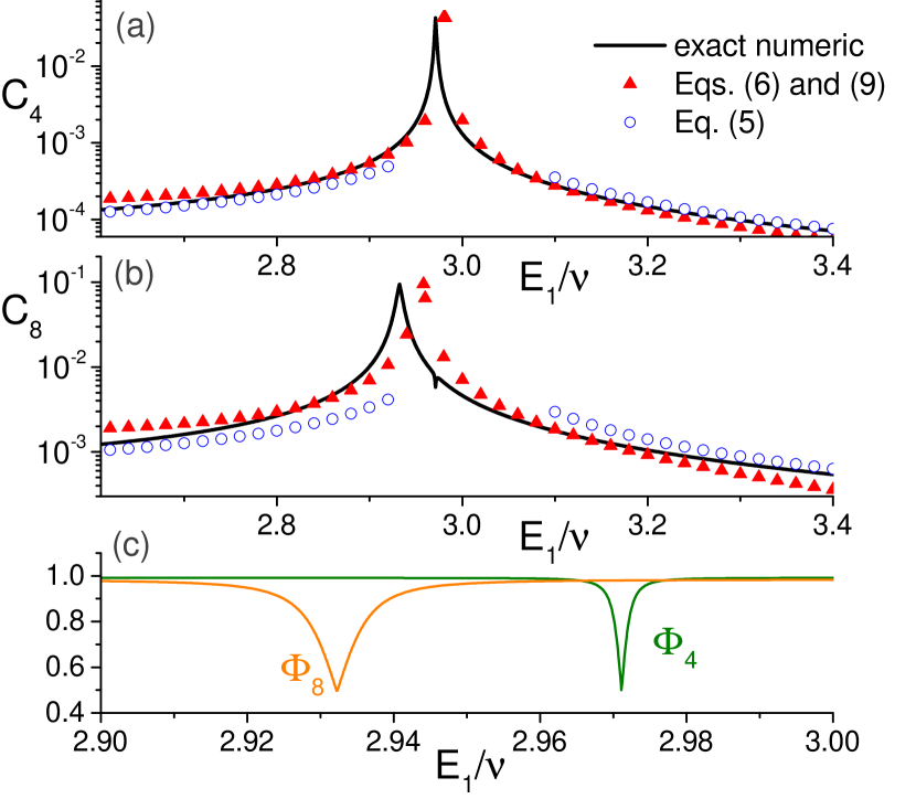
Figure 1: (color online) a) Matrix element $C_{4}$ as function of the qubit’s frequency. Solid line represent the exact numeric evaluation; red triangles correspond to approximate analytic expressions (7) and (10) valid near the 3-photon resonance $E_{1}\approx 3\nu$; blue circles depict Eq. (6) valid far from $E_{1}\approx 3\nu$. b) Matrix element $C_{8}$. c) Exact numeric evaluation of the fidelity $\Phi_{m}\equiv|\langle\mathbf{0},m|\varphi_{0,m}\rangle|^{2}$ for $m=4$ and $8$.

First it is analyzed the qubit with a realistic cQED7 coupling strength $g_{1}=0.08\nu$. The behavior of the two lowest matrix elements $C_{4}\equiv|C_{0,0;0,4}|$ and $C_{8}\equiv|C_{0,4;0,8}|$ as function of the qubit’s frequency is shown in Figs. 1a-b. The exact values (solid lines) were obtained through numeric diagonalization of the Hamiltonian $\hat{H}_{0}$. Blue circles stand for the analytical formula (6) valid far from the three-photon resonance $E_{1}\approx 3\nu$, and the red triangles correspond to the expressions (7) and (10) applicable near this resonance. Although the perturbative approach is questionable for the assumed large ratio $g_{1}/\nu$, there is a good agreement between exact and approximate results. The main quantitative discrepancy is a slight displacement in the location of the three-photon resonances, expected analytically for $4\nu=\beta_{k+4}+\beta_{k+2}$. Fig. 1c presents the exact results for the fidelity $\Phi_{m}\equiv|\langle\mathbf{0},m|\varphi_{0,m}\rangle|^{2}$ that measures the weight of the state $|\mathbf{0},m\rangle$ in the dressed-state $|\varphi_{0,m}\rangle$, for $m=4$ and $8$. As expected, in the strong dispersive regime $\Phi_{m}=1/2$ at the three-photon resonances and $\Phi_{m}\approx 1$ otherwise. This confirms that near $E_{1}\approx 3\nu$ it is possible to implement 4DCE with the vacuum transition rate $|\Theta_{0,0;0,4}|\lesssim 10^{-2}\varepsilon g_{1}/\nu$.

Fig. 2a illustrates the unitary dynamics for parameters $E_{1}=2.968\nu$ and $\eta=3.9819\nu$, obtained by solving numerically the Schrödinger equation. $\langle n\rangle$ is the average photon number, $P_{a}(k)$ is the population of the atomic level $|\mathbf{k}\rangle$ and $Q=[\langle(\Delta n)^{2}\rangle-\langle n\rangle]/\langle n\rangle$ is the Mandel’s factor of the cavity field. Several photons are generated from vacuum via effective four-photon transitions, while the qubit remains mainly in the ground state. At certain times the $Q$-factor becomes negative, implying sub-Poissonian field statistics, while at other times it can assume large ratios, $Q/\langle n\rangle\sim 10$. Such behavior is easily understood by looking at the evolution of the field in the Fock basis. The largest photon-number probabilities $p(m)=\mathrm{Tr}[|m\rangle\langle m|\hat{\rho}]$ are displayed in Fig. 2c, where $\hat{\rho}$ is the total density operator. $Q<0$ corresponds to the system approximately in the state $|\mathbf{0},8\rangle$, while the case $Q\gg\langle n\rangle$ occurs when the state $|\mathbf{0},0\rangle$ dominates but there are small populations of states $|\mathbf{0},8\rangle$ and $|\mathbf{1},1\rangle$. The denomination “four-photon dynamical Casimir effect” (4DCE) seems appropriate to describe this phenomenon, since only the states $|\mathbf{0},4\rangle$, $|\mathbf{0},8\rangle$ and $|\mathbf{0},12\rangle$ become significantly populated, although the population of the state $|\mathbf{0},12\rangle$ is quite low due to the effective Kerr nonlinearity [last term in Eq. (11)]. Due to the proximity to three-photon resonance, there is also a slight occupation of the near-degenerate state $|\mathbf{1},1\rangle$, as seen from the low-amplitude oscillations of $P_{a}(0)$ and $p(1)$.

One can grasp the main qualitative effects of weak dissipation by solving numerically the phenomenological master equation at zero temperature bla (see Refs. diego ; palermo for the discussion on its validity in similar situations)

$$\dot{\rho}=\frac{1}{i\hbar}[\hat{H},\hat{\rho}]+\kappa\mathcal{L}[\hat{a}]+\gamma\mathcal{L}[\hat{\sigma}_{0,1}]+\frac{\gamma_{\phi}}{2}\mathcal{L}[\hat{\sigma}_{z}]\,\,.$$

Here $\hat{\sigma}_{z}\equiv\hat{\sigma}_{1,1}-\hat{\sigma}_{0,0}$, $\mathcal{L}[\hat{O}]\equiv\hat{O}\hat{\rho}\hat{O}^{\dagger}-\hat{O}^{\dagger}\hat{O}\hat{\rho}/2-\hat{\rho}\hat{O}^{\dagger}\hat{O}/2$ is the Lindblad superoperator, $\kappa$ is the cavity relaxation rate and $\gamma$ ($\gamma_{\phi}$) is the atomic relaxation (pure dephasing) rate. Fig. 2b illustrates the behavior of $\langle n\rangle$, $Q$ and $P_{a}(0)$ for feasible feas1 ; feas2 dissipative parameters $\gamma=\gamma_{\phi}=5\times 10^{-4}g_{1}$ and $\kappa=10^{-4}g_{1}$. The main message is that several photons can still be generated from vacuum, and for initial times the dissipative behavior closely resembles the unitary one. For large times the cavity relaxation leads to excitation of all the Fock states with $m\lesssim 10$, so it is not surprising that the behavior is altered drastically.

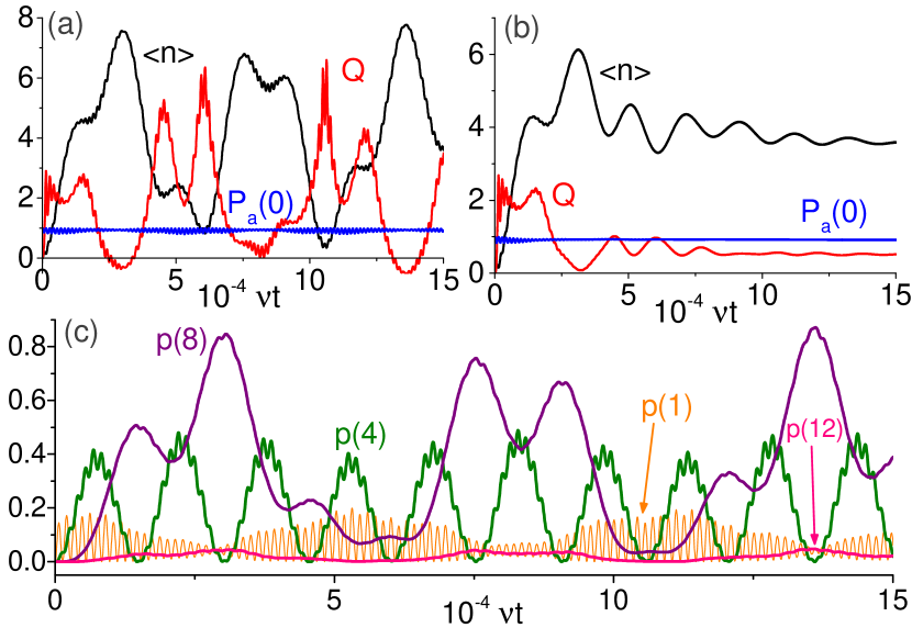
Figure 2: (color online) a) Unitary dynamics of 4DCE for parameters $E_{1}=2.968\nu$ and $\eta=3.9819\nu$. b) Dynamics in the presence of weak Markovian dissipation. c) Behavior of the most populated cavity Fock states under unitary evolution.

As was shown in Fig. 1, minor changes of $E_{1}$ in the vicinity of three-photon resonance strongly affect the transition rates. This feature is illustrated in Fig. 3, where the parameters of Fig. 2 were slightly changed to $E_{1}=2.99\nu$ and $\eta=3.\,\allowbreak 9821\nu$. The new behavior is completely different: only the states $|\mathbf{0},0\rangle$ and $|\mathbf{0},4\rangle$ become significantly populated throughout the evolution; $p(8)$ attains at most 0.04 (making the maximum value of $\langle n\rangle$ slightly larger than 4), and all other populations are even smaller. The photon creation is slower than in Fig. 2, nonetheless, the phenomenon can still occur in the presence of weak dissipation.

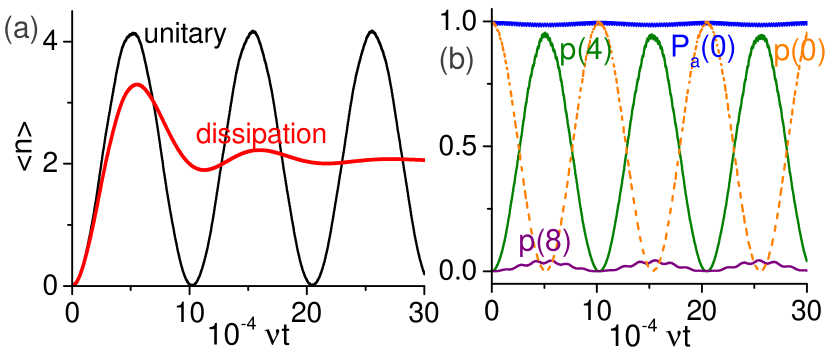
Figure 3: (color online) a) Average photon number with and without dissipation for parameters $E_{1}=2.99\nu$, $\eta=3.\,\allowbreak 9821\nu$. b) Ground state population of the qubit, $P_{a}(0)$, and the largest photon number probabilities $p(k)$ during unitary evolution.

V.2 5-photon DCE

At last the cyclic qutrit is investigated, assuming coupling strengths $g_{1}=6\times 10^{-2}\nu$, $g_{2}=8\times 10^{-2}\nu$ and $g_{3}=4\times 10^{-2}\nu$. Fig. 4a displays the matrix elements $C_{3}\equiv|C_{0,0;0,3}|$, $C_{5}\equiv|C_{0,0;0,5}|$ and $C_{10}\equiv|C_{0,5;0,10}|$ as function of $E_{1}/\nu$ for $\Delta_{2}=0$ (for other values of $\Delta_{2}$ the behavior is qualitatively similar). The dressed-states $|\varphi_{0,m}\rangle$ (which contain the largest contribution of the state $|\mathbf{0},m\rangle$) were obtained via exact numeric diagonalization of the Hamiltonian $\hat{H}_{0}$. As predicted in Sec. IV, the vacuum transition rate for 5DCE ($C_{5}$) is usually 2 orders of magnitude smaller than for 3DCE $(C_{3}$). However, near certain atomic frequencies there is a resonant enhancement of the transition rate, and 5DCE becomes almost as strong as 3DCE. Fig. 4b shows the fidelities $\Phi_{m}$ for $m=3$, $5$ and $10$. As expected, as long as one stays far from $E_{1}\approx\nu$ and slightly off the resonance conditions $\tilde{\lambda}_{0,n}=\tilde{\lambda}_{S/A,n-l}$, the fidelities are very close to 1, allowing for the resonant enhancement of the transition rate without significantly exciting the atom. It is also worth noting that the linewidths of the peaks of $C_{m}$ become narrower as $E_{1}$ increases, requiring high-precision tuning of the atomic energy levels in addition to the modulation frequency.

Fig. 4c illustrates how the peak-value $C_{5}^{(\max)}$ (associated with 5DCE from vacuum) scales with $\Delta_{2}/\nu$, where the atomic energy $E_{1}$ was adjusted according to the requirement $\tilde{\lambda}_{0,5}=\tilde{\lambda}_{S/A,5-l}$ for $l=3$ and $4$, denoted by the pair of indexes $\{S/A,l\}$ [the case $l=2$ is not shown since the corresponding rate is one order of magnitude smaller, in agreement with Eqs. (18) and (21)]. Black thick lines denote the exact numeric results, and the thin lines correspond to Eqs. (19) – (23). The agreement is excellent, and one can see that for the chosen parameters the optimum transition rates occur for $|\Delta_{2}|\gtrsim 0.2\nu$. Finally, Fig. 4d illustrates the dependence of the resonant value $E_{1}^{(res)}$ that maximizes $C_{5}$ as function of $\Delta_{2}/\nu$. Analytic results (thin lines) correspond to Eqs. (15) – (16), and are in excellent agreement with the exact numeric results (thick black lines).

Figure 4: (color online) a) Matrix elements $C_{m}$ as function of $E_{1}/\nu$ for $\Delta_{2}=0$. b) Fidelities $\Phi_{m}$ for $\Delta_{2}=0$. c) Peak-values $C_{5}^{(\max)}$ as function of $\Delta_{2}/\nu$, where $\{S/A,l\}$ denotes de condition $\tilde{\lambda}_{0,5}=\tilde{\lambda}_{S/A,5-l}$. Thick (thin) lines describe the numeric (analytic) results. d) Values of $E_{1}^{(res)}/\nu$ (for which $C_{5}$ is maximum) as function of $\Delta_{2}$.

Figure 5: (color online) a) 5DCE for parameters $E_{1}=3.105\nu$, $E_{2}=4.08\nu$ and $\eta=4.9842\nu$. In the left panel the scale for $\langle n\rangle$ and  $Q$ is on the left axis, while the scale for $1-P_{a}(0)$ is on the right axis. The right panel depicts the most populated cavity Fock states. b) Similar analysis for $E_{1}=2.2\nu$, $E_{2}=3.05\nu$ and $\eta=4.\,\allowbreak 9732\nu$, when at most $5$ photons are created.

Actual examples of unitary dynamics are illustrated in Fig. 5, as obtained via numeric solution of the Schrödinger equation. In panel 5a the parameters are $E_{1}=3.105\nu$, $E_{2}=4.08\nu$ and $\eta=4.\,\allowbreak 9842\nu$. The plotted quantities are $\langle n\rangle$, $Q$, $1-P_{a}(0)$ and the most populated cavity Fock states. Both $p(1)$ and $p(2)$ are very small and have the same order of magnitude, so the quantity $p(1)+p(2)$ is plotted instead. In agreement with Eq. (17), $p(1)+p(2)$ almost coincides with $1-P_{a}(0)$, since at the resonance the states $|\mathbf{0},5\rangle$, $|\mathbf{1},2\rangle$ and $|\mathbf{2},1\rangle$ are nearly degenerate. The most populated states are $|\mathbf{0},5\rangle$ and $|\mathbf{0},10\rangle$, with other states $|\mathbf{0},5k\rangle$ almost unpopulated due to the mismatch between the modulation frequency $\eta$ and $(\lambda_{0,5k}-\lambda_{0,5k-5})$ for $k>2$. In Fig. 5b similar analysis is carried for $E_{1}=2.2\nu$, $E_{2}=3.05\nu$ and $\eta=4.\,\allowbreak 9732\nu$. Now at most $5$ photons are created from vacuum, but due to the proximity to the resonance peak of $C_{5}$ the states $|\mathbf{1},3\rangle$ and $|\mathbf{2},2\rangle$ also become populated, which explains why $\langle n\rangle$ never attains the value $5$ and why $P_{a}(1)$ and $P_{a}(2)$ deviate significantly from zero.

VI Conclusions

The problem of a single-mode cavity with harmonically modulated frequency was revisited in the presence of a qubit or a cyclic qutrit. It was found analytically that the counter-rotating terms in the light-matter interaction Hamiltonian allow for photon generation from vacuum via effective 4- and 5-photon processes for qubit and cyclic qutrit, respectively, while the atom remains approximately in the ground state. Usually the associated transition rates are very small, but they undergo a resonant enhancement by orders of magnitude in the strong dispersive regime near certain atomic frequencies. For the qubit such resonance occurs near $E_{1}\approx 3\nu$, while for the qutrit there are six resonance conditions that depend on both $E_{1}$ and $E_{2}$. Due to the effective Kerr nonlinearity, only a limited number of photons can be generated for a constant modulation frequency. Besides, dissipation alters drastically the dynamics after some time due to the population of cavity Fock states forbidden by unitary evolution. Nonetheless, for weak dissipation and sufficiently strong modulation amplitude, $\varepsilon/\nu\gtrsim 10^{-3}$, 4- and 5-photon DCE could be implemented experimentally for modulation frequencies $\eta\approx 4\nu$ and $\eta\approx 5\nu$, respectively.

References

• (1) G. T. Moore, Quantum theory of electromagnetic field in a variable-length one-dimensional cavity, J. Math. Phys. 11, 2679 (1970).
• (2) V. V. Dodonov, Nonstationary Casimir Effect and analytical solutions for quantum fields in cavities with moving boundaries, in Modern Nonlinear Optics, Advances in Chemical Physics Series, Vol. 119, part 1, edited by M. W. Evans (Wiley, New York, 2001), pp. 309–394.
• (3) V. V. Dodonov, Current status of the dynamical Casimir effect, Phys. Scr. 82, 038105 (2010).
• (4) D. A. R. Dalvit, P. A. Maia Neto, and F.D.Mazzitelli, Fluctuations, dissipation and the dynamical Casimir effect, in Casimir Physics, edited by D. Dalvit, P. Milonni, D. Roberts, and F. da Rosa, Lecture Notes in Physics Vol. 834 (Springer, Berlin, 2011), pp. 419–457.
• (5) P. D. Nation, J. R. Johansson, M. P. Blencowe, and F. Nori, Colloquium: Stimulating uncertainty: Amplifying the quantum vacuum with superconducting circuits, Rev. Mod. Phys. 84, 1 (2012).
• (6) A. Lambrecht, M. T. Jaekel and S. Reynaud, Motion Induced Radiation from a vibrating cavity, Phys. Rev. Lett. 77, 615 (1996).
• (7) A. Lambrecht, M. T. Jaekel and S. Reynaud, Frequency up-converted radiation from a cavity moving in vacuum, Eur. Phys. J. D 3, 95 (1998).
• (8) S. A. Fulling and P. C. W. Davies, Radiation from a moving mirror in two dimensional space-time: Conformal Anomaly, Proc. R. Soc. London A 348, 393 (1976).
• (9) G. Barton and C. Eberlein, On quantum radiation from a moving body with finite refractive index, Ann. Phys. (NY) 227, 222 (1993).
• (10) P. A. Maia Neto and L. A. S. Machado, Quantum radiation generated by a moving mirror in free space, Phys. Rev. A 54, 3420 (1996).
• (11) P. LΓ€hteenmΓ€ki, G. S. Paraoanu, J. Hassel, and P. J. Hakonen, Dynamical Casimir effect in a Josephson metamaterial, Proc. Natl. Acad. Sci. USA 110, 4234 (2013).
• (12) C. K. Law, Effective Hamiltonian for the radiation in a cavity with a moving mirror and a time-varying dielectric medium, Phys. Rev. A 49, 433 (1994).
• (13) A. V. Dodonov, E. V. Dodonov and V. V. Dodonov, Photon generation from vacuum in nondegenerate cavities with regular and random periodic displacements of boundaries, Phys. Lett. A 317, 378 (2003).
• (14) E. L. S. Silva and A. V. Dodonov, Analytical comparison of the first- and second-order resonances for implementation of the dynamical Casimir effect in nonstationary circuit QED, J. Phys. A: Math. Theor. 49, 495304 (2016).
• (15) V. V. Dodonov, Photon creation and excitation of a detector in a cavity with a resonantly vibrating wall, Phys. Lett. A 207, 126 (1995).
• (16) V. V. Dodonov and A. B. Klimov, Generation and detection of photons in a cavity with a resonantly oscillating boundary, Phys. Rev. A 53, 2664 (1996).
• (17) A. V. Dodonov, Continuous intracavity monitoring of the dynamical Casimir effect, Phys. Scr. 87, 038103 (2013).
• (18) D. S. Veloso and A. V. Dodonov, Prospects for observing dynamical and antidynamical Casimir effects in circuit QED due to fast modulation of qubit parameters, J. Phys. B: At. Mol. Opt. Phys. 48, 165503 (2015).
• (19) L. C. Monteiro and A. V. Dodonov, Anti-dynamical Casimir effect with an ensemble of qubits, Phys. Lett. A 380, 1542 (2016).
• (20) Y.-X. Liu, J. Q. You, L. F. Wei, C. P. Sun, and F. Nori, Optical selection rules and phase-dependent adiabatic state control in a superconducting quantum circuit, Phys. Rev. Lett. 95, 087001 (2005).
• (21) Y.-X. Liu, H.-C. Sun, Z. H. Peng, A. Miranowicz, J. S. Tsai, and F. Nori, Controllable microwave three-wave mixing via a single three-level superconducting quantum circuit, Sci. Rep. 4, 7289 (2014).
• (22) Y.-J. Zhao, J.-H. Ding, Z. H. Peng, and Y.-X. Liu, Realization of microwave amplification, attenuation, and frequency conversion using a single three-level superconducting quantum circuit, Phys. Rev. A 95, 043806 (2017).
• (23) P. Zhao, X. Tan, H. Yu, S.-L. Zhu, and Y. Yu, Circuit QED with qutrits: Coupling three or more atoms via virtual-photon exchange, Phys. Rev. A 96, 043833 (2017).
• (24) X. Gu, A. F. Kockum, A. Miranowicz, Y. X. Liu, and F. Nori, Microwave photonics with superconducting quantum circuits, Phys. Rep. 718-719, 1 (2017).
• (25) H. Dessano and A. V. Dodonov, One- and three-photon dynamical Casimir effects using a nonstationary cyclic qutrit, Phys. Rev. A 98, 022520 (2018).
• (26) The distinction between the instantaneous and fixed annihilation and creation operators is neglected here, assuming that the measurements are made after the perturbation has ceased.
• (27) S. De Liberato, D. Gerace, I. Carusotto, and C. Ciuti, Extracavity quantum vacuum radiation from a single qubit, Phys. Rev. A 80, 053810 (2009).
• (28) W. P. Schleich, Quantum Optics in Phase Space (Berlin: Wiley, 2001).
• (29) A. V. Dodonov, A. Napoli and B. Militello, Emulation of n-photon Jaynes-Cummings and anti-Jaynes-Cummings models via parametric modulation of a cyclic qutrit, Phys. Rev. A 99, 033823 (2019).
• (30) K. K. W. Ma and C. K. Law, Three-photon resonance and adiabatic passage in the large-detuning Rabi model, Phys. Rev. A 92, 023842 (2015).
• (31) F. Beaudoin, J. M. Gambetta and A. Blais, Dissipation and ultrastrong coupling in circuit QED, Phys. Rev. A 84, 043832 (2011).
• (32) A. V. Dodonov, B. Militello, A. Napoli, and A. Messina, Effective Landau-Zener transitions in the circuit dynamical Casimir effect with time-varying modulation frequency, Phys. Rev. A 93, 052505 (2016).
• (33) A. Megrant et al., Planar superconducting resonators with internal quality factors above one million, Appl. Phys. Lett. 100, 113510 (2012).
• (34) Y. Lu et al., Universal stabilization of a parametrically coupled qubit, Phys. Rev. Lett. 119, 150502 (2017).