HINT: Hierarchical Invertible Neural Transport
for Density Estimation and Bayesian Inference

Abstract

Many recent invertible neural architectures are based on coupling block designs where variables are divided in two subsets which serve as inputs of an easily invertible (usually affine) triangular transformation. While such a transformation is invertible, its Jacobian is very sparse and thus may lack expressiveness. This work presents a simple remedy by noting that subdivision and (affine) coupling can be repeated recursively within the resulting subsets, leading to an efficiently invertible block with dense, triangular Jacobian. By formulating our recursive coupling scheme via a hierarchical architecture, HINT allows sampling from a joint distribution $p(\mathbf{y},\mathbf{x})$ and the corresponding posterior $p(\mathbf{x}\,|\,\mathbf{y})$ using a single invertible network. We evaluate our method on some standard data sets and benchmark its full power for density estimation and Bayesian inference on a novel data set of 2D shapes in Fourier parameterization, which enables consistent visualization of samples for different dimensionalities.

Introduction

Invertible neural networks based on the normalizing flow principle have recently gained increasing attention for generative modeling, in particular networks built on a coupling block design (Dinh, Sohl-Dickstein, and Bengio 2017). Their success is due to a number of useful properties: (a) they can tractably model complex high-dimensional probability densities without suffering from the curse-of-dimensionality, (b) training via the maximum likelihood objective is generally very stable, (c) their latent space opens up opportunities for model interpretation and manipulation, and (d) the same trained model can be used for both efficient data generation and efficient density calculation.

While autoregressive models can also be trained as normalizing flows and share properties (a) and (b), they sacrifice efficient invertibility for expressive power and thus lose properties (c) and (d). In contrast, lack of expressive power of a single invertible block is a core limitation of invertible networks, which needs to be compensated by extremely deep models with dozens or hundreds of blocks, e.g., the GLOW architecture (Kingma and Dhariwal 2018). While invertibility allows to back-propagate through very deep networks with minimal memory footprint (Gomez et al. 2017), more expressive invertible building blocks are still of great interest. The superior performance of autoregressive approaches such as (Van den Oord et al. 2016) is due to the stronger interaction between variables, reflected in a dense triangular Jacobian matrix, at the expense of cheap inversion. The theory of transport maps (Villani 2008) provides certain guarantees of universality for triangular maps, which do not hold for the standard coupling block design with a comparatively sparse Jacobian (figure 1, left).

Figure 1: Sparse (left) and dense (right) triangular Jacobian of a standard coupling block and of our recursive design, respectively. Nonzero parts of the Jacobian in gray.

Here, we propose an extension to the coupling block design that recursively fills in the previously unused portions of the Jacobian using smaller coupling blocks. This allows for dense triangular maps (figure 1, right), or any intermediate design if the recursion is stopped before, while retaining the advantages of the original coupling block architecture. Furthermore, the recursive structure of this mapping can be used for efficient conditional sampling and Bayesian inference. Splitting the variables of interest into two subsets $\mathbf{x}$ and $\mathbf{y}$, a single normalizing flow model can be built that allows efficient sampling from both the joint distribution $p(\mathbf{x},\mathbf{y})$ and the conditional $p(\mathbf{x}\,|\,\mathbf{y})$. It should be noted that our extension would also work for convolutional architectures like GLOW.

Finally, we introduce a new family of data sets based on Fourier parameterizations of two-dimensional curves. In the normalizing flow literature, there is an abundance of two-dimensional toy densities that provide an easy visual check for correctness of the model output. However, the sparsity of the basic coupling block only becomes an issue beyond two dimensions where it is challenging to visualize the distribution or individual samples. Pixel-based image data sets, on the other hand, quickly are too high dimensional for a meaningful assessment of the quality of the estimated densities.

A step towards visualizable data sets of intermediate size has been made in (Kruse et al. 2019), but their four-dimensional problems are still too simple to demonstrate the advantages of the recursive coupling approach described above. To fill the gap, we describe a way to generate data sets of arbitrary dimension, where each data point parameterizes a closed curve in 2D space that is easy to visualize. Increasing the input data dimension allows the representation of distributions of more and more complex curves.

To summarize, the contributions of this paper are: (a) a simple, efficiently invertible flow model with dense, triangular Jacobian; (b) a hierarchical architecture to model joint as well as conditional distributions; (c) a novel family of data sets allowing easy visualization for arbitrary dimensions.

The remainder of this work consists of a literature review, some mathematical background, a description of our method and supporting numerical experiments, followed by closing remarks.

Related Work

Normalizing flows were popularized in the context of deep learning chiefly by the work of (Rezende and Mohamed 2015) and (Dinh, Krueger, and Bengio 2015). By now, a large variety of architectures exist to realize normalizing flows. The majority falls into one of two groups: coupling block architectures and autoregressive models. For a comprehensive overview and background information on invertible neural networks and normalizing flows see (Kobyzev, Prince, and Brubaker 2019) or (Papamakarios et al. 2019).

Additive and then affine coupling blocks were first introduced by (Dinh, Krueger, and Bengio 2015; Dinh, Sohl-Dickstein, and Bengio 2017), while (Kingma and Dhariwal 2018) went on to generalize the permutation of variables between blocks by learning the corresponding matrices, besides demonstrating the power of flow networks as generators. Subsequent works have focused on replacing the (componentwise) affine transformation at the heart of such networks, which limits expressiveness, e.g., by replacing affine couplings with more expressive monotonous splines (Durkan et al. 2019), albeit at the cost of evaluation speed.

On the other hand, there is lso a rich body of work on autoregressive (flow) networks (Huang et al. 2018; Kingma et al. 2016; Van den Oord et al. 2016; Van den Oord, Kalchbrenner, and Kavukcuoglu 2016; Papamakarios, Pavlakou, and Murray 2017). More recently, (Jaini, Selby, and Yu 2019) applied second-order polynomials to improve expressive power over typical autoregressive models and proved that their model is a universal density approximator. While such models provide excellent density estimation compared to coupling architectures (Liao, He, and Shu 2019; Ma et al. 2019), generating samples is often not a priority and can be prohibitively slow.

There are other approaches, outside those two subfields, that also seek a favorable trade-off between expressive power and efficient invertibility. Residual Flows (Behrmann et al. 2019; Chen et al. 2019) impose Lipschitz constraints on a standard residual block, which guarantees invertibility with a full Jacobian and enables approximate maximum-likelihood training but requires an iterative procedure for sampling. Similarly, (Song, Meng, and Ermon 2019) uses lower triangular weight matrices that can be inverted via fixed-point iteration. The normalizing flow principle is formulated continuously as a differential equation (DE) by (Grathwohl et al. 2019), which allows free-form Jacobians but requires integrating a DE for each network pass. (Karami et al. 2019) introduce another method with dense Jacobian, based on invertible convolutions in the Fourier domain.

In terms of modeling conditional densities with invertible neural networks, (Ardizzone et al. 2019a) proposed an approach that divides the network output into conditioning variables and a latent vector, training the flow part with a maximum mean discrepancy objective (MMD, Gretton et al. 2012) instead of maximum likelihood. Later (Ardizzone et al. 2019b) introduced a simple conditional coupling block to construct a conditional normalizing flow.

Mathematical Background

For an input vector $\mathbf{x}\in\mathbb{R}^{N}$, a standard, invertible coupling block is abstractly defined by

$$\mathbf{x}^{\prime}=f_{\text{C}}(\mathbf{x})=\begin{bmatrix}\mathbf{x}_{1}\\ C\big{(}\mathbf{x}_{2}\,|\,\mathbf{x}_{1}\big{)}\end{bmatrix}=\begin{bmatrix}\mathbf{x}^{\prime}_{1}\\ \mathbf{x}^{\prime}_{2}\end{bmatrix},$$ (1)

where $\mathbf{x}_{1}=\mathbf{x}_{0:\lfloor N/2\rfloor}$ and $\mathbf{x}_{2}=\mathbf{x}_{\lfloor N/2\rfloor:N}$ are the first and second half of the input vector and $\mathbf{x}^{\prime}_{2}=C(\mathbf{x}_{2}\,|\,\mathbf{x}_{1})$ is an easily invertible transform of $\mathbf{x}_{2}$ conditioned on $\mathbf{x}_{1}$. Its inverse is then simply given by

$$\mathbf{x}=f_{\text{C}}^{\sminus 1}(\mathbf{x}^{\prime})=\begin{bmatrix}\mathbf{x}^{\prime}_{1}\\ C^{\sminus 1}\big{(}\mathbf{x}^{\prime}_{2}\,|\,\mathbf{x}^{\prime}_{1}\big{)}\end{bmatrix}.$$ (2)

For affine coupling blocks (Dinh, Sohl-Dickstein, and Bengio 2017), $C$ takes the form $C(\mathbf{u}\,|\,\mathbf{v})=\mathbf{u}\odot\exp\big{(}s(\mathbf{v})\big{)}+t(\mathbf{v})$ with $s$ and $t$ unconstrained feed-forward networks. The logarithm of the Jacobian determinant of such a block can be computed very efficiently as

$$\log\big{|}\det\mathbf{J}_{f_{\text{C}}}(\mathbf{x})\big{|}=\log\left|\det\frac{\partial f_{\text{C}}(\mathbf{x})}{\partial\mathbf{x}}\right|=\text{sum}(s\!\left(\mathbf{x}_{1}\right)).$$ (3)

To ensure that all entries of $\mathbf{x}$ are transformed and interact with each other, a pipeline that alternates between coupling blocks and random orthogonal matrices $\mathbf{Q}$ is constructed, where the orthogonal block $\mathbf{x}^{\prime}=f_{\mathbf{Q}}(\mathbf{x})=\mathbf{Qx}$ can trivially be inverted as $\mathbf{x}=f^{\sminus 1}_{\mathbf{Q}}(\mathbf{x}^{\prime})=\mathbf{Q}^{\top}\mathbf{x}^{\prime}$ with log-determinant $\log\left|\det\mathbf{J}_{f_{\mathbf{Q}}}(\mathbf{x})\right|=0$.

Normalizing Flows and Transport Maps

To create a normalizing flow, this ‘pipeline’ $T=f_{\text{C}1}\circ f_{\mathbf{Q}1}\circ f_{\text{C}2}\circ f_{\mathbf{Q}2}\circ\ldots$ is trained via maximum likelihood loss

$$\mathcal{L}(\mathbf{x})=\tfrac{1}{2}\|T(\mathbf{x})\|_{2}^{2}-\log\left|\mathbf{J}_{T}(\mathbf{x})\right|$$ (4)

to transport the data distribution $p_{X}$ to a standard normal latent distribution $p_{Z}=\mathcal{N}(\mathbf{0},\mathbf{I})$. The map $T$ can then be used to sample from $p_{X}$ by drawing a sample $\mathbf{z}^{(i)}$ from $p_{Z}$ in the latent space and by passing it through the inverse model $S=T^{\sminus 1}$ to obtain $\mathbf{x}^{(i)}=S(\mathbf{z}^{(i)})$.

Using the change-of-variables formula, the density at a given data point $\mathbf{x}$ can also be calculated as $p_{X}(\mathbf{x})=p_{Z}(T(\mathbf{x}))\cdot\left|\det\mathbf{J}_{T}(\mathbf{x})\right|$. The mathematical basis of this procedure is the theory of transport maps (Villani 2008), which are employed in exactly the same way to push a reference density (e.g. Gaussian) to a target density (e.g. the data distribution, (Marzouk et al. 2016)). In fact, up to a constant, namely the (typically inaccessible) fixed entropy $H(p_{X})$ of the data distribution, the expected value of the objective in equation 4 is the Kullback-Leibler (KL) divergence between the data distribution $p_{X}$ and the push-forward of the latent density $S_{\#}p_{Z}$:

$$D_{\text{KL}}(p_{X}\,\|\,S_{\#}p_{Z}) =\int p_{X}(\mathbf{x})\log\frac{p_{X}(\mathbf{x})}{S_{\#}p_{Z}(\mathbf{x})}\,\text{d}\mathbf{x}$$

$$=\mathbb{E}_{\mathbf{x}\sim p_{X}}[\mathcal{L}(\mathbf{x})]+H(p_{X}).$$ (5)

Normalizing flows represent one parametrised family of maps over which equation 4 can be minimized. Other examples include polynomial (Marzouk et al. 2016), kernel-based (Liu and Wang 2016) or low-rank tensor (Dolgov et al. 2020) approximations.

Note also that each pair $f_{\text{C}i}\circ f_{\mathbf{Q}i}$ in $T$ is a composition of an orthogonal transformation and a triangular map, where the latter is better known in the field of transport maps as a Knothe-Rosenblatt rearrangement (Marzouk et al. 2016). This can be interpreted as a non-linear generalization of the classic QR decomposition (Stoer and Bulirsch 2013). Whereas the triangular part encodes the possibility to represent non-linear transformations, the orthogonal part reshuffles variables to foster dependence of each part of the input to the final output, thereby drastically increasing the representational power of the map $T$.

Bayesian Inference with Conditional Flows

Inverse problems arise when one possesses a well-understood model for the forward mapping $\mathbf{x}\rightarrow\mathbf{y}$ from hidden parameters $\mathbf{x}$ to observable outcomes $\mathbf{y}$, e.g. in the form of an explicit likelihood $p(\mathbf{y}\,|\,\mathbf{x})$ or a Monte-Carlo simulation. However, the actual object of interest is the inverse mapping $\mathbf{y}\rightarrow\mathbf{x}$ from observations to parameters. According to Bayes’ theorem, this requires estimation of the posterior conditional density $p(\mathbf{x}\,|\,\mathbf{y})$. Such Bayesian inference problems arise frequently in the sciences and are generally very hard.

Normalizing flows can be used in several ways to estimate conditional densities. The approach in this paper is inspired by (Marzouk et al. 2016) and exploits the link to Knothe-Rosenblatt maps highlighted above. As described below, see figure 3 (left), it suffices to constrain the possible rearrangements of variables in the coupling blocks, i.e. the choice of the orthogonal blocks $f_{\mathbf{Q}i}$, to enable conditional sampling. This was first noted in (Detommaso et al. 2019).

Independently, (Ardizzone et al. 2019b) and (Winkler et al. 2019) introduced conditional coupling blocks that allow an entire normalizing flow to be conditioned on external variables. By conditioning the transport $T$ between $p_{X}(\mathbf{x})$ and $p_{Z}(\mathbf{z})$ on the corresponding values of $\mathbf{y}$ as $\mathbf{z}=T(\mathbf{x}\,|\,\mathbf{y})$, its inverse $T^{\sminus 1}(\mathbf{z}\,|\,\mathbf{y})$ can be used to turn the latent distribution $p_{Z}(\mathbf{z})$ into an approximation of the posterior $p(\mathbf{x}\,|\,\mathbf{y})$.

Method

We extend the basic coupling block design in two ways.

The Recursive Coupling Block

As visualized in figure 1 (left), the Jacobian $\mathbf{J}_{f}$ of a simple coupling block is very sparse, i.e. many possible interactions between variables are not modelled. However the efficient determinant computation in equation 3 works for any lower triangular $\mathbf{J}_{f}$, and indeed theorem 1 of (Hyvärinen and Pajunen 1999) states that a single triangular transformation can, in theory, already represent arbitrary distributions.

The following recursive coupling scheme $f_{\text{R}}$ makes use of this potential and fills the empty areas below the diagonal: Given $\mathbf{x}\in\mathbb{R}^{N}$ and a hierarchy depth $K\in\mathbb{N}$, we define recursively, for $k=K,K-1,\ldots,1$:

$$\mathbf{x}^{\prime}=f_{\text{R},k}(\mathbf{x})= f_{\text{C}}(\mathbf{x}), N_{k}\!\leq\!3$$ if ,

$$\mathbf{x}^{\prime}=f_{\text{R},k}(\mathbf{x})= \begin{bmatrix}f_{\text{R},k\sminus 1}(\mathbf{x}_{1})\\ C_{k}\left(f_{\text{R},k\sminus 1}\big{(}\mathbf{x}_{2}\big{)}\,\middle|\,\mathbf{x}_{1}\right)\end{bmatrix},$$ else, (6)

where for each $k$, $\mathbf{x}_{1}=\mathbf{x}_{0:\lfloor N_{k}/2\rfloor}$ and $\mathbf{x}_{2}=\mathbf{x}_{\lfloor N_{k}/2\rfloor:N_{k}}$, $N_{k}$ is the size of the current input vector and $N_{K}=N$. Note that each sub-coupling has its own coupling function $C_{k}$ with independent parameters. The inverse transform is

$$\mathbf{x}=f^{\sminus 1}_{\text{R},k}(\mathbf{x}^{\prime})\!=\!\begin{cases}f^{\sminus 1}_{\text{C}}(\mathbf{x}^{\prime}),\hfill\text{if }N_{k}\leq 3,\\ \!\begin{bmatrix}f^{\sminus 1}_{\text{R},k\sminus 1}(\mathbf{x}^{\prime}_{1})\\ f^{\sminus 1}_{\text{R},k\sminus 1}\!\left(C_{k}^{\sminus 1}\!\left(\mathbf{x}^{\prime}_{2}\,\middle|\,f^{\sminus 1}_{\text{R},k\sminus 1}(\mathbf{x}^{\prime}_{1})\right)\right)\end{bmatrix}\!,\text{ else}.\end{cases}$$ (7)

For $K=\lceil\log_{2}N\rceil$, this procedure leads to the dense lower triangular Jacobian visualized in figure 1 (right), the log-determinant of which is simply the sum of the log-determinants of all sub-couplings $C_{k}$. A visual representation of the architecture can be seen in figure 2.

Figure 2: A recursive affine coupling block. The inner functions $f_{\text{R}}(\mathbf{x}_{i})$ take again the form of the outer gray block, repeated until the maximum hierarchy depth is reached. Each such coupling block in itself has a triangular Jacobian.

Figure 3: Top: Single HINT block with recursive coupling, and its Jacobian matrix. Transformation of $\mathbf{x}$ is influenced by $\mathbf{y}$, but not vice-versa, imposing a hierarchy on variables. Bottom: Using HINT flows for conditional sampling/Bayesian inference.

However, since the (sub-)coupling blocks are affine, $f_{\text{R},K}$ can only represent an approximation of the exact Knothe-Rosenblatt map and it is still necessary, as for standard coupling blocks, to create a normalizing flow by composing several recursive coupling blocks interspersed with orthogonal transformations $f_{\mathbf{Q}}$. Thus, in practice, it is also more economical to limit the depth of the hierarchy to 2 or 3. This already increases the amount of interaction between individual variables considerably, while limiting the computational overhead, but it allows to use much shallower networks. The trade-off between number of blocks and hierarchy depth will be studied for the Fourier shapes data set in this work.

Hierarchical Invertible Neural Transport

While the recursive coupling block defined above is motivated by the search for a more expressive architecture, it is also ideally suited for estimating conditional flows and thus for Bayesian inference.

Specifically, in a setting with paired data $(\mathbf{x}_{i},\mathbf{y}_{i})$, where subsequently we want a sampler for $\mathbf{x}$ conditioned on $\mathbf{y}$, we can provide both variables as input to the flow, separating them in the first hierarchy level for further transformation at the next recursion level. Crucially, $\mathbf{x}$ and $\mathbf{y}$ variables are never permuted between lanes, thus only feeding forward information from the $\mathbf{y}$-lane to the $\mathbf{x}$-lane as shown in figure 3 (top left). Instead of one large permutation operation over all variables, as in the hierarchical coupling block design in figure 2, we apply individual permutations $\mathbf{Q}_{\mathbf{y}}$ and $\mathbf{Q}_{\mathbf{x}}$ to each respective lane at the beginning of the block. A normalizing flow model constructed in this way performs hierarchical invertible neural transport, or HINT for short.

The output of a HINT model is a latent code with two components, $\mathbf{z}=[\mathbf{z}_{\mathbf{y}},\mathbf{z}_{\mathbf{x}}]^{\top}=T(\mathbf{y},\mathbf{x})$, but the training objective stays the same as in equation 4:

$$\mathcal{L}(\mathbf{y},\mathbf{x})=\tfrac{1}{2}\|T(\mathbf{y},\mathbf{x})\|_{2}^{2}-\log\left|\mathbf{J}_{T}(\mathbf{y},\mathbf{x})\right|$$ (8)

As with a standard normalizing flow, the joint density of input variables is the pull-back of the latent density via $T$:

$$p_{T}(\mathbf{y},\mathbf{x})=S_{\#}p_{Z}(\mathbf{z})=S_{\#}\mathcal{N}(\mathbf{0},\mathbf{I}_{|\mathbf{y}|+|\mathbf{x}|}),$$ (9)

where $S=T^{-1}$. But because the $\mathbf{y}$-lane in HINT can be evaluated independently of the $\mathbf{x}$-lane, we can determine the partial latent code $\mathbf{z}_{\mathbf{y}}$ for a given $\mathbf{y}$ and hold it fixed (figure 3, bottom left), while drawing $\mathbf{z}_{\mathbf{x}}$ from the $\mathbf{x}$-part of the latent distribution (bottom right). This yields samples from the conditional density:

$$\mathbf{x}=S^{\mathbf{x}}([\mathbf{z}_{\mathbf{y}},\mathbf{z}_{x}])\sim p_{T}(\mathbf{x}\,|\,\mathbf{y})\quad\text{with }\mathbf{z}_{\mathbf{y}}=T^{\mathbf{y}}(\mathbf{y}),$$ (10)

where superscripts $\mathbf{x}$ and $\mathbf{y}$ respectively denote $\mathbf{x}$- and $\mathbf{y}$-lanes of the transformations. This means HINT gives access to both the joint density of $\mathbf{x}$ and $\mathbf{y}$, as well as the conditional density of $\mathbf{x}$ given $\mathbf{y}$, e.g. for Bayesian inference.

Computational Complexity

The number of couplings doubles in every recursion level, whereas the workload per coupling decreases exponentially, so that the total order of complexity of HINT and RealNVP is the same. All sub-networks $s$ and $t$ within one level are independent of each other and can be processed in a single parallel pass on the GPU (see appendix). Only the final affine transformations and some bookkeeping operations must be executed sequentially, but at negligible cost compared to the other tensor operations. Our first, non-parallel implementation of HINT is 2-10 times slower than RealNVP.

Experiments

We perform experiments on classical UCI data sets (Dua and Graff 2017) and a new data set called “Fourier shapes”. We introduce this new data set to balance four conflicting goals:

1. The dimension of the data should be high enough for HINT’s hierarchical decomposition to make a difference.

2. The dimension should be low enough to allow for accurate quantitative evaluation and comparison of results.

3. Learning the joint distribution should be challenging due to complex interactions between variables.

4. Visualizations should allow intuitive qualitative comparison of the differences between alternative approaches.

Our new data set represents families of 2-dimensional contours in terms of the probability density of their Fourier coefficients and fulfills the above requirements: The dimension of the problem can be easily adjusted by controlling the complexity of the shapes under consideration and the number of Fourier coefficients (1,2). Shapes with sharp corners and long-range symmetries require accurate alignment of many Fourier coefficients (specifically, of their phases, 3 – see appendix). Humans can readily recognize the quality of a shape representation in a picture (4).

Our experiments show considerable improvements of HINT over RealNVP. To clearly demonstrate these advantages, we heavily restrict the networks’ parameter budgets – larger networks would be much more accurate, but exhibit less meaningful differences. Models were trained on an RTX 2080 Ti GPU. Hyper-parameters are listed in the appendix.

UCI Density Estimation Benchmarks

The tabular UCI data sets (Dua and Graff 2017) are popular for comparing density models. Using public code for pre-processing, we compare several flow models with Real-NVP and recursive coupling blocks in terms of the average log-likelihood on the test set. To tease out shortcomings, each model is “handicapped” to a budget of 500k (Power, Gas) or 250k (Miniboone) trainable parameters.

Table 1 shows that the recursive design achieves similar or better test likelihood in all cases, even when the low dimensionality (Dim) of the data allows little recursion.

Blocks		Dim	Real-NVP	Recursive
	Power	6	$-0.054$ p m 0.017	$-0.027$ p m 0.018
4	Gas	8	$7.620$ p m 0.136	$7.662$ p m 0.094
	Miniboone	42	$-19.296$ p m 0.395	$-14.547$ p m 0.164
	Power	6	$0.093$ p m 0.002	$0.080$ p m 0.007
8	Gas	8	$8.062$ p m 0.177	$8.137$ p m 0.055
	Miniboone	42	$-16.625$ p m 0.119	$-14.117$ p m 0.163

Table 1: Normal and recursive coupling compared on UCI benchmarks in terms of average log-likelihood (mean $\pm$ std over 3 training runs; higher is better $\uparrow$).

Fourier Shapes Data Set

A curve $\mathbf{g}(t)\in\mathbb{R}^{2}$, parameterized by $2M\!+\!1$ complex 2d Fourier coefficients $\mathbf{a}_{m}\in\mathbb{C}^{2}$, can be traced as

$$\mathbf{g}(t)=\textstyle\sum_{m=-M}^{M}\mathbf{a}_{m}\cdot e^{2\pi\cdot i\cdot m\cdot t}$$ (11)

with parameter $t$ running from $0$ to $1$. This parameterization will always yield a closed, possibly self-intersecting curve (McGarva and Mullineux 1993).

Vice-versa, we can calculate the Fourier coefficients

$$\mathbf{a}_{m}=\frac{1}{L}\sum_{l=0}^{L-1}\mathbf{p}_{l}\cdot e^{-2\pi\cdot i\cdot m\cdot l/L},\ \text{for}\;m\in[-M,M],$$ (12)

to approximately fit a curve through a sequence of $L$ points $\mathbf{p}_{l}\in\mathbb{R}^{2}$, $l=0,\ldots,L-1$. By increasing $M$, higher order terms are added to the parameterization in equation 11 and the shape is approximated in greater detail. An example of this effect for a natural shape is shown in figure 4 (right). Note that the actual dimensionality of the parameterization in our data set is $|\mathbf{x}|=4\cdot(2M+1)$, as each complex 2d coefficient $\mathbf{a}_{m}$ is represented by four real numbers.

Figure 4: Left: A 2d polygon obtained from the segmentation of a natural image. Middle: The vertices $\mathbf{p}_{l}$ of the polygon forming the basis for computing the Fourier coefficients in equation 12. Right: Tracing the curve $\mathbf{g}(t)$ according to equation 11, for different numbers $M$ of Fourier terms $\mathbf{a}_{m}$.

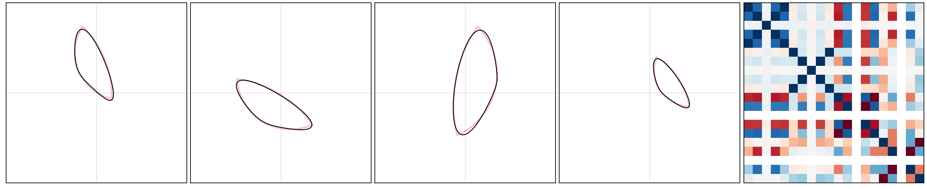
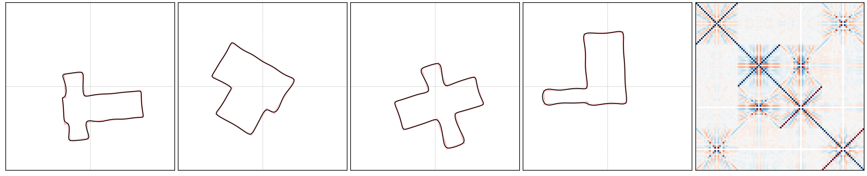
Figure 5: Left: Samples from the Lens shapes data set, and true correlation matrix of Fourier coefficients for a large batch of Lens shapes. Right: The same for Cross shapes. Red lines behind the Fourier curves show the original geometry they approximate.

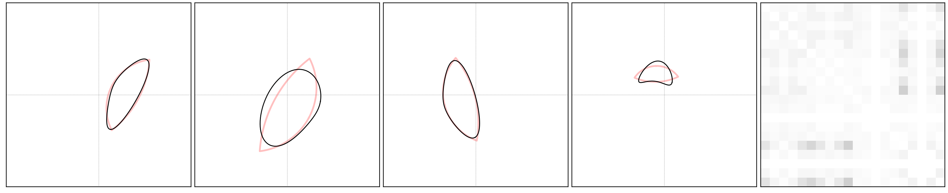
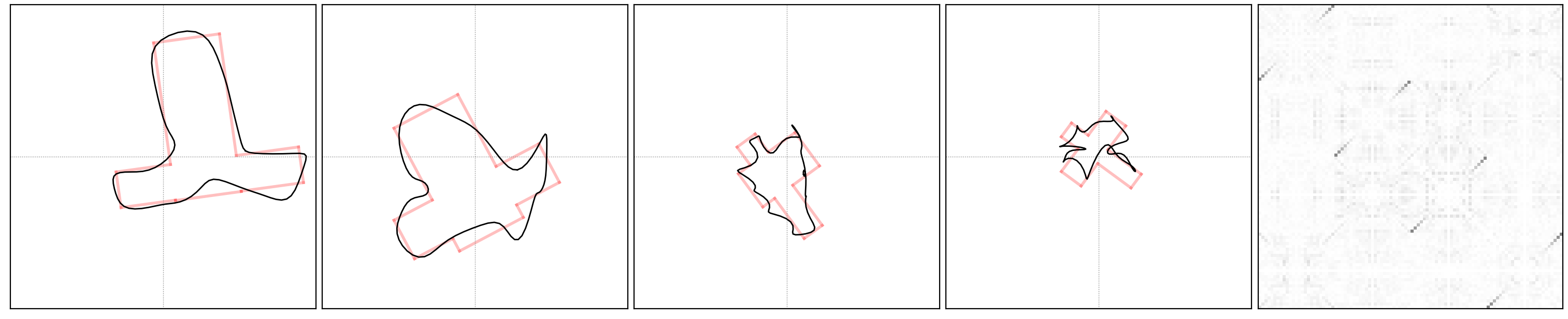
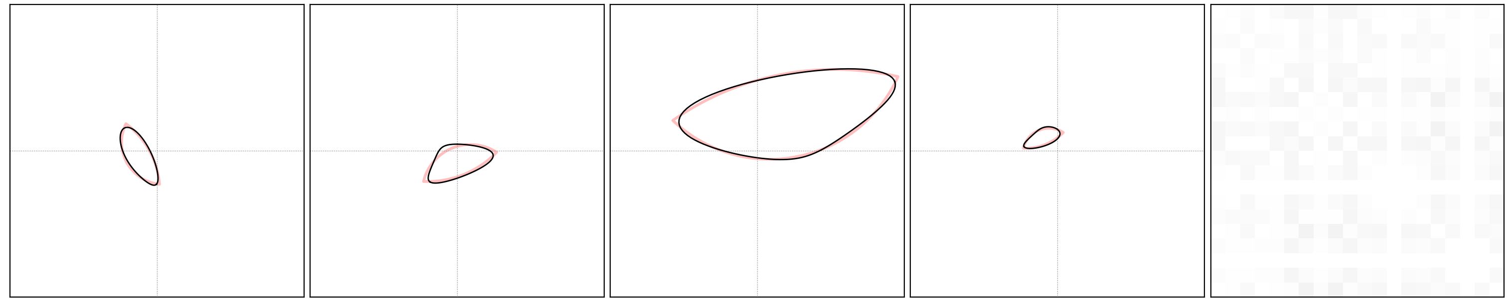
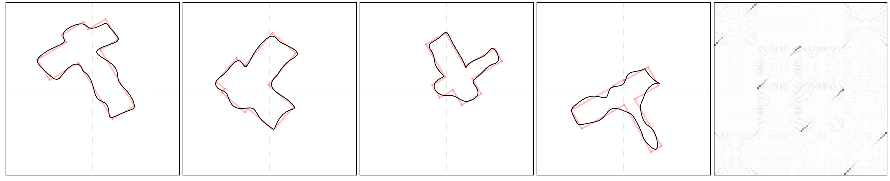
Figure 6: Samples from Real-NVP (top) and recursive (bottom) coupling block networks, trained on the Lens shapes (left) and the Cross shapes (right) from figure 5. The closest fitting shapes from the true distributions are depicted in red for reference. Here and in subsequent figures, the fifth panel shows the absolute differences between true and sampling correlation matrices.

We perform experiments on two specific data sets, first using curves of order $M=2$, i.e. $|\mathbf{x}|=20$, to represent a distribution of simple shapes that arise from the intersection of two randomly placed circles with a fixed ratio of radii and a fixed distance. The resulting Lens shapes can be seen in figure 5 (left), together with the highly structured correlation matrix of Fourier parameters $\mathbf{x}_{i}$ that yield such shapes.

The second data set uses $M=12$, i.e. $|\mathbf{x}|=100$, to represent Cross shapes which are generated by crossing two bars of random length, width and lateral shift at a right angle, oriented randomly, but positioned close to the origin. This results in a variation of Xs, Ls and Ts, some of which are shown in figure 5 (right) together with the even more complicated ($100\times 100$) parameter correlation matrix.

Density estimation.

For density estimation, a single-block and a two-block network are trained on the Lens-shapes data, once with standard coupling blocks and once with the new recursive design. All networks have the same total parameter budget – details in the appendix.

Samples from the two-block models and absolute differences to the true parameter correlation matrices are shown in figure 6 (left). Qualitatively, samples from the recursive model are visually more faithful and have smaller errors in the correlation matrices. Quantitatively, we compare over three training runs per model using the following metrics:

• Maximum mean discrepancy (MMD, Gretton et al. 2012) measures the dissimilarity of two distributions using only samples from both. Following (Ardizzone et al. 2019a), we use MMD with an inverse multi-quadratic kernel and average the results over $100$ batches from the data prior and from each trained model. Lower is better.

• Average log-likelihood (LL) of the test data under the model, i.e. $-\tfrac{1}{2}T(\mathbf{x})^{2}+\text{log}|\mathbf{J}_{T}(\mathbf{x})|-\text{log}(2\pi\tfrac{N}{2})$ where $N$ is the data dimensionality. Higher is better.

• Average intersection-over-union (IoU) between generated shapes and the best fitting shape that follows the construction rules of the data set. See appendix for details on the fitting procedure. Higher is better.

• Average Hausdorff distance (H-dist) between the contours of the generated shapes and those of the best fitting shapes, as above. Lower is better.

Table 2 shows how recursive coupling blocks outperform the conventional design. The difference is especially striking for the single-block network, as a non-recursive coupling block leaves half the variables untouched and is thus inherently unable to model the data distribution properly.

We also trained standard and recursive networks with 4 and 8 coupling blocks on the larger Cross-shapes data set. Representative samples from the 4-block models are shown in figure 6 (right) together with the best fitting, actual Cross shape. Here, it is even more clearly visible that the recursive model produces samples with better geometry, i.e right angles, straight lines and symmetries in the expected locations.

A quantitative comparison in terms of LL, IoU and H-dist is presented in table 3, with recursive coupling consistently outperforming standard Real-NVP blocks.

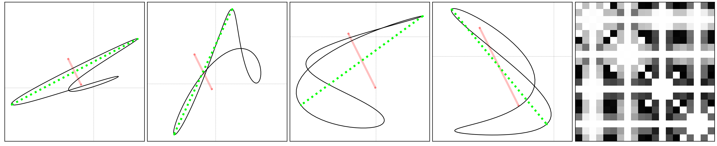
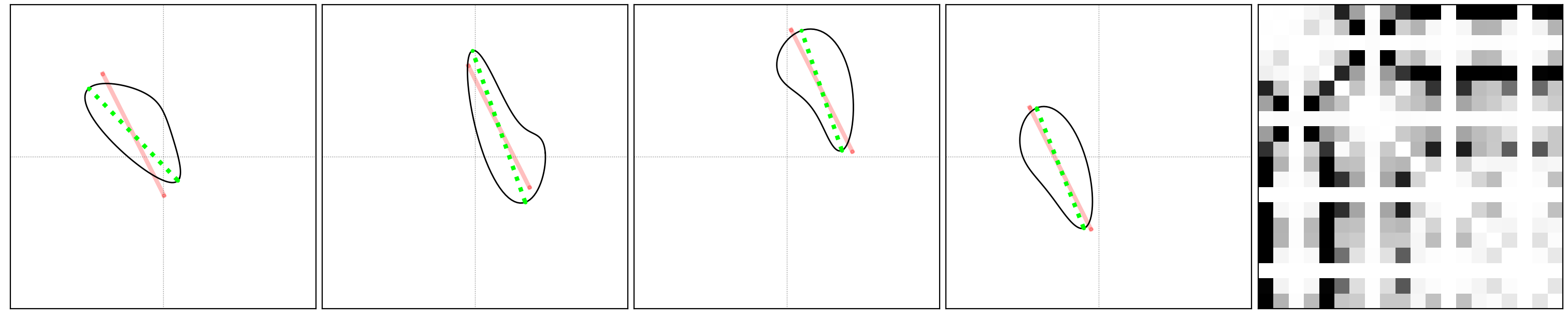
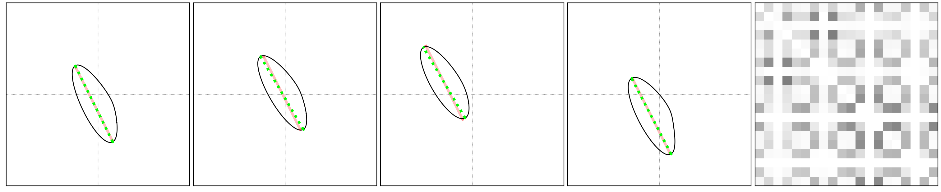
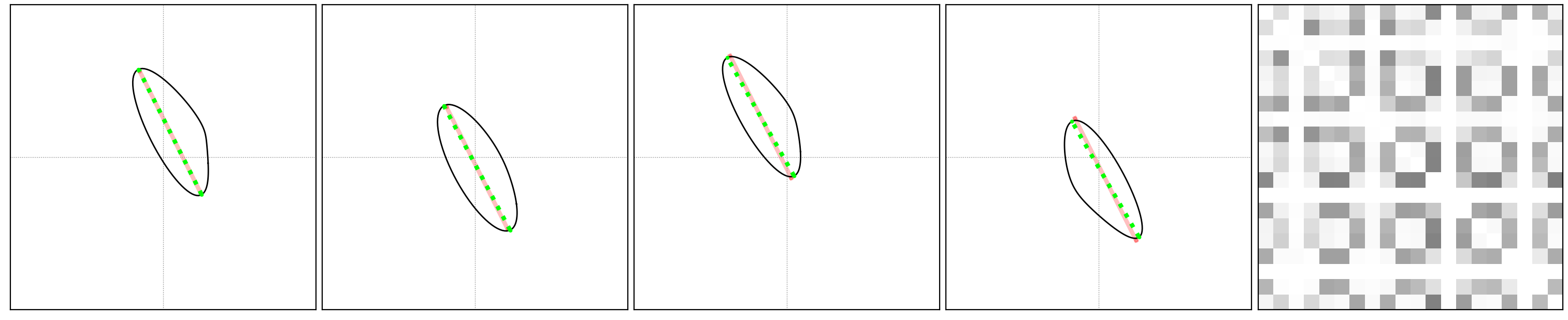
Figure 7: Samples from a conditional coupling net (cINN, left) and from HINT (right), trained Lens shapes. Green dotted lines mark the largest diameter of each shape; red lines show how it should look according to the data $\mathbf{y}$. Both models do well with 4 blocks (bottom), but only HINT generates reasonable samples with a single coupling block (top). Last panels as in figure 6.

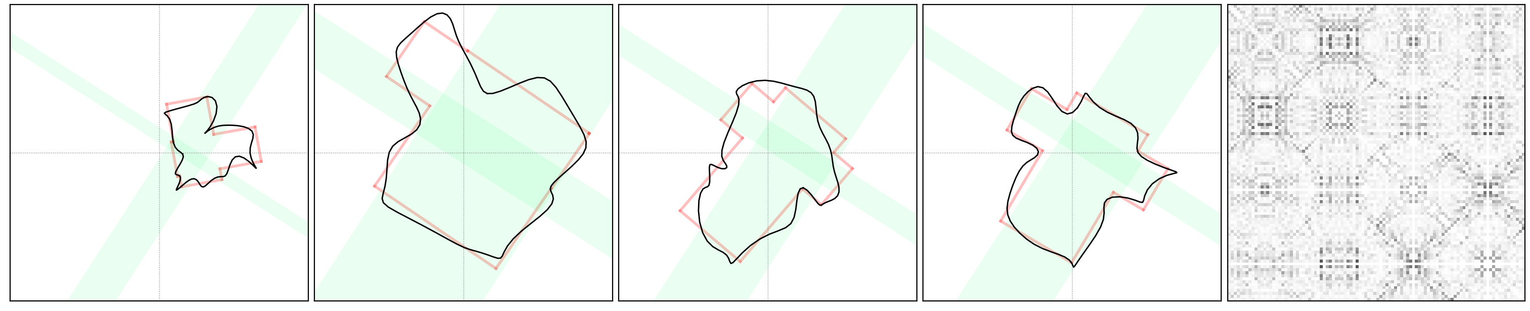
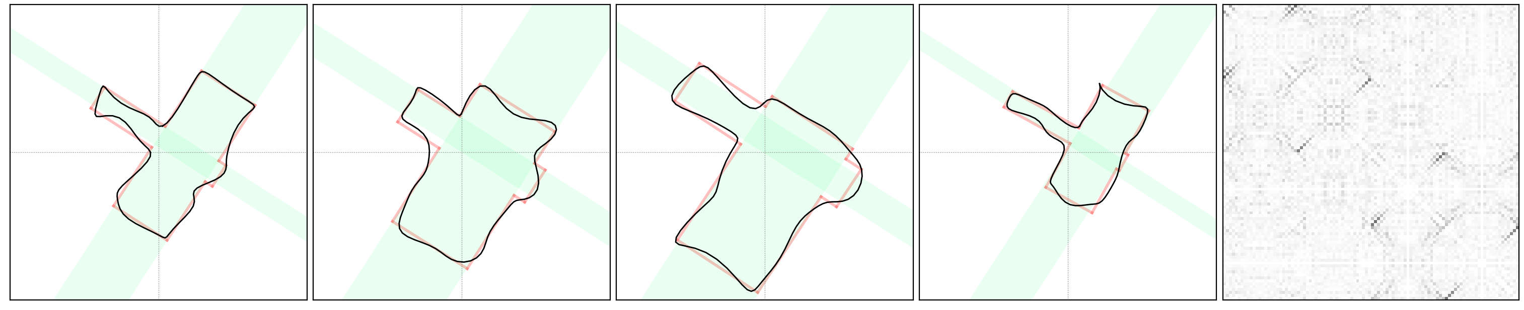
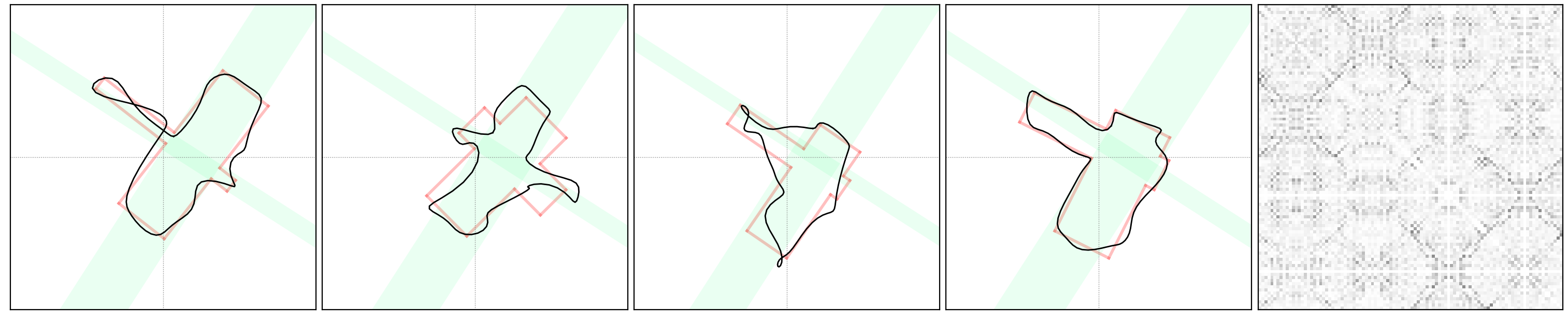
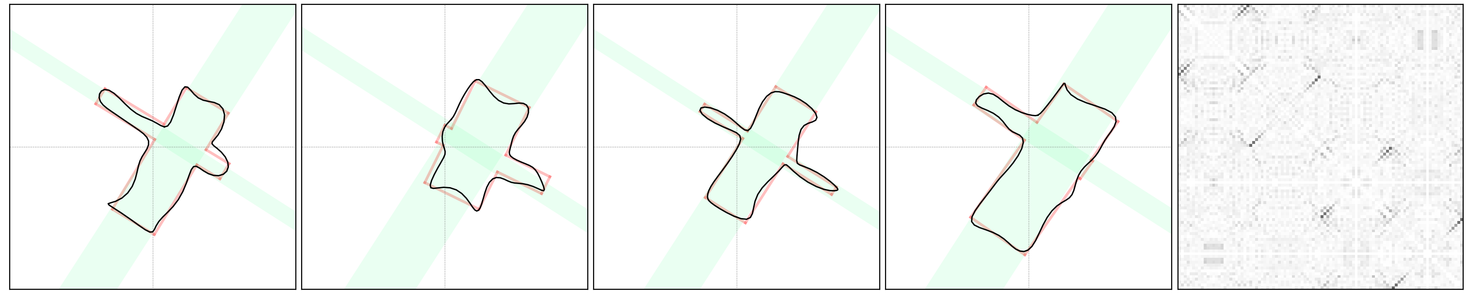
Figure 8: Samples from a conditional coupling net (cINN, left) and from HINT (right) with 4 (top) or 8 (bottom) blocks, trained on Cross shapes. The expected center, angle and thickness ratio of the Cross according to the data $\mathbf{y}$ are shown in green, the best fitting Cross shape in red. Visually, HINT reproduces shapes from the data set much better. Last panels as in figure 6.

Blocks		Real-NVP	Recursive
	MMD $\downarrow$	$0.370$ p m 0.000	$0.140$ p m 0.002
1	LL $\uparrow$	$2.021$ p m 0.001	$2.861$ p m 0.006
	IoU $\uparrow$	$0.449$ p m 0.010	$0.688$ p m 0.014
	H-dist $\downarrow$	$0.519$ p m 0.005	$0.109$ p m 0.005
	MMD $\downarrow$	$0.012$ p m 0.001	$0.009$ p m 0.004
2	LL $\uparrow$	$3.141$ p m 0.036	$3.219$ p m 0.005
	IoU $\uparrow$	$0.789$ p m 0.024	$0.819$ p m 0.006
	H-dist $\downarrow$	$0.063$ p m 0.007	$0.057$ p m 0.000

Table 2: Comparing Real-NVP and recursive coupling for sampling and density estimation for the Lens-shapes data (plotting mean $\pm$ standard deviation over 3 training runs).

Bayesian Inference on Fourier Shapes

To set-up Bayesian inference tasks, we formulate forward mappings $\mathbf{x}\rightarrow\mathbf{y}$ from $\mathbf{x}$ to observable features $\mathbf{y}$. Since these features are incomplete shape descriptors, the inverse $\mathbf{y}\rightarrow\mathbf{x}$ is ambiguous, and $p(\mathbf{x}\,|\,\mathbf{y})$ is learned with HINT.

Given a Lens shape, our forward mapping locates its two tips and returns their horizontal and vertical distances $d_{h}$ and $d_{v}$. The tips’ absolute positions and the side of the lens’ “bulge” remain undetermined by these features.

The forward mapping for Cross shapes returns four geometrical features. These are the 2d coordinates of the center, i.e where the bars cross, plus the angle of and thickness ratio between the two bars. What remains free, are the absolute thickness, as well as the length and lateral shift of the bars.

Finally, noise $\sigma\sim\mathcal{N}(\mathbf{0},\tfrac{1}{20}\mathbf{I})$ is added to the output of each forward mapping to obtain observed data vectors $\mathbf{y}$.

We trained a conditional flow model (cINN) and HINT with 1, 2, 4 and 8 blocks for Bayesian inference on the Lens shapes. A quantitative comparison, in terms of MMD, IoU and H-dist, is given in table 4. Here, however, MMD does not compare to samples from the prior $p_{X}(\mathbf{x})$, but to samples from an estimate of the true posterior $p(\mathbf{x}\,|\,\mathbf{y})$, estimated via Approximate Bayesian Computation (ABC, Csilléry et al. 2010), as in (Ardizzone et al. 2019a), see appendix.

Blocks	$4\times$ rnvp	$4\times$ rec	$8\times$ rnvp	$8\times$ rec
LL $\uparrow$	$3.419$	$3.627$	$3.329$	$3.637$
IoU $\uparrow$	$0.594$	$0.823$	$0.588$	$0.823$
H-dist $\downarrow$	$0.134$	$0.077$	$0.138$	$0.073$

Table 3: Comparison of flow models for Cross shapes with normal (rnvp) and recursive coupling (rec), respectively.

Blocks		cINN	HINT
	MMD $\downarrow$	$0.746$ p m 0.000	$0.030$ p m 0.001
1	IoU $\uparrow$	$0.456$ p m 0.001	$0.849$ p m 0.003
	H-dist $\downarrow$	$0.521$ p m 0.006	$0.051$ p m 0.001
	MMD $\downarrow$	$0.048$ p m 0.012	$0.016$ p m 0.001
2	IoU $\uparrow$	$0.839$ p m 0.011	$0.869$ p m 0.005
	H-dist $\downarrow$	$0.054$ p m 0.002	$0.044$ p m 0.002
	MMD $\downarrow$	$0.020$ p m 0.003	$0.010$ p m 0.001
4	IoU $\uparrow$	$0.865$ p m 0.006	$0.875$ p m 0.007
	H-dist $\downarrow$	$0.046$ p m 0.002	$0.043$ p m 0.002
	MMD $\downarrow$	$0.007$ p m 0.002	$0.011$ p m 0.003
8	IoU $\uparrow$	$0.864$ p m 0.003	$0.876$ p m 0.003
	H-dist $\downarrow$	$0.046$ p m 0.001	$0.043$ p m 0.001

Table 4: Conditional (cINN) vs. hierarchical (HINT) coupling for Bayesian inference on Lens shapes (mean $\pm$ standard deviation over 3 training runs). See text for details.

In table 4 we see that HINT consistently produces better shapes (measured by IoU and H-dist), especially in the case of a single block, and it exhibits better conditioning (as evidenced by MMD) for all but the 8-block model, most likely due to the limited parameter budget, which leaves some of the sub-networks underparameterized. A similar effect can be observed in the LL (not shown in table 4), when only measuring the log-likelihood of the $\mathbf{x}$-lane in HINT and simply excluding contributions from the $\mathbf{y}$-lane.

Qualitative results in figures 7 and 8, for the Lens and for the Cross shapes, respectively, confirm the superior performance of HINT also visually, in particular producing significantly better angles and symmetries for the Cross shapes. This is quantitatively supported in the metrics in table 5.

Blocks	$4\times\!$ cINN	$4\times\!$ HINT	$8\times\!$ cINN	$8\times\!$ HINT
LL $\uparrow$	$3.625$	$3.724$	$3.609$	$3.766$
IoU $\uparrow$	$0.654$	$0.843$	$0.590$	$0.859$
H-dist $\downarrow$	$0.116$	$0.073$	$0.119$	$0.066$

Table 5: Fidelity of Cross shapes generated by conditional (cINN) and hierarchical (HINT) flows, respectively.

Recursion Depth vs. Number of Blocks

Seeing that recursive coupling blocks outperform standard ones, we also tested if using more standard coupling blocks closes the gap. We looked at several combinations of number of blocks, recursion depth and parameter budget on the Cross-shapes data. In summary, the first two recursion levels improve performance more than additional coupling blocks. Beyond that, we see diminishing returns, as the limited parameter budget gets distributed over too many subnetworks. Full results are in the appendix.

Conclusion

We presented recursive coupling blocks and HINT, a new invertible architecture for normalizing flow, improving on the traditional coupling block in terms of expressive power by densifying the triangular Jacobian, while keeping the advantages of an accessible latent space. This keeps the efficient sampling and density estimation of RealNVP, which is often compromised by other approaches to denser Jacobians, e.g. auto-regressive flows. To evaluate the model, we introduced a versatile family of data sets based on Fourier decompositions of simple 2D shapes that can be visualized easily, independent of the chosen dimension. In terms of future improvements, we expect that our formulation can be made more computationally efficient through the use of e.g. masking operations, enabling more advanced parallelization.

– APPENDIX –

Figure 9: Configurations for initializing the shape fitting algorithm on Cross shapes, with a given angle.

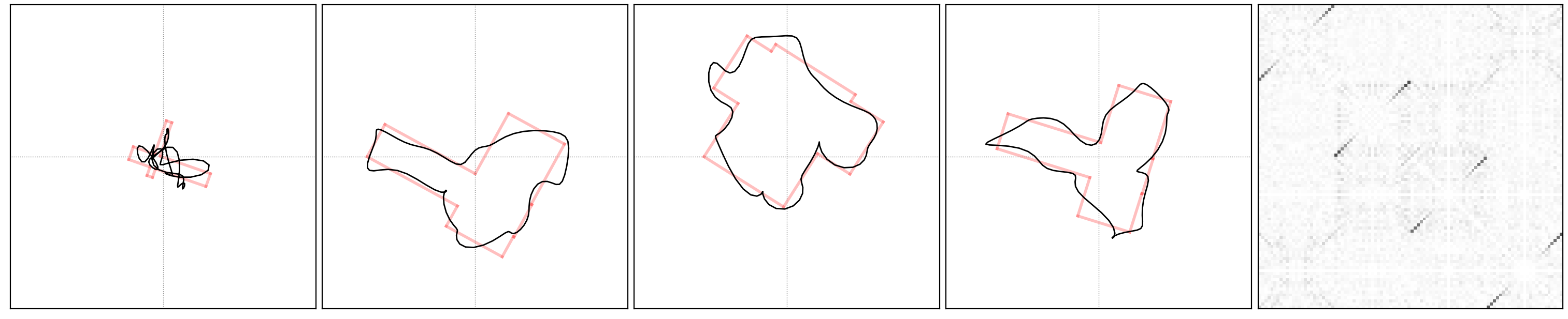
(a) Real-NVP, 8 blocks:

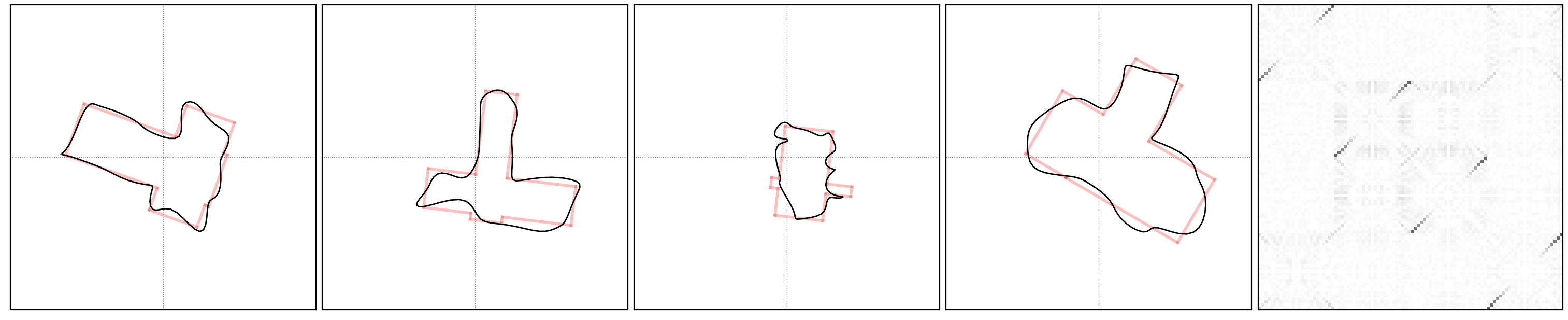
(b) Real-NVP, 16 blocks:

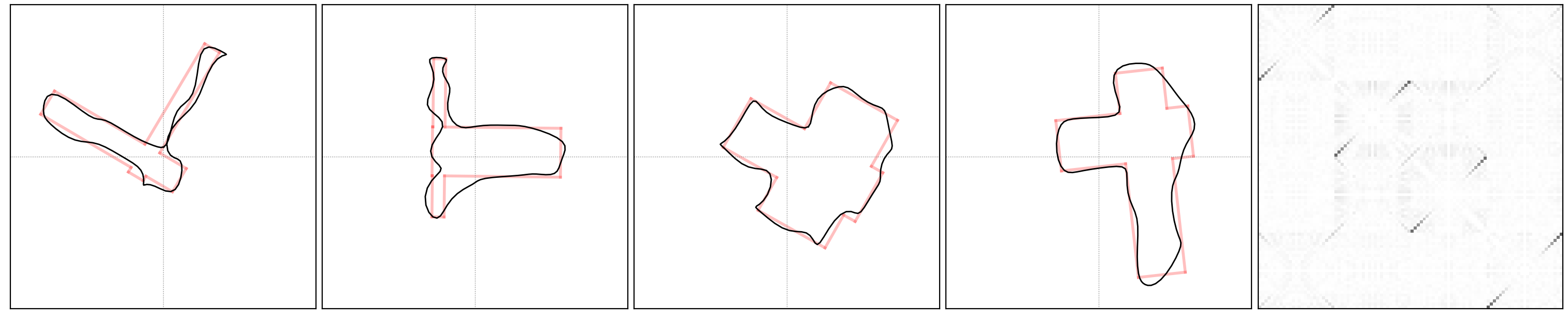
(c) Real-NVP, 32 blocks:

(d) Recursive coupling, 4 blocks:

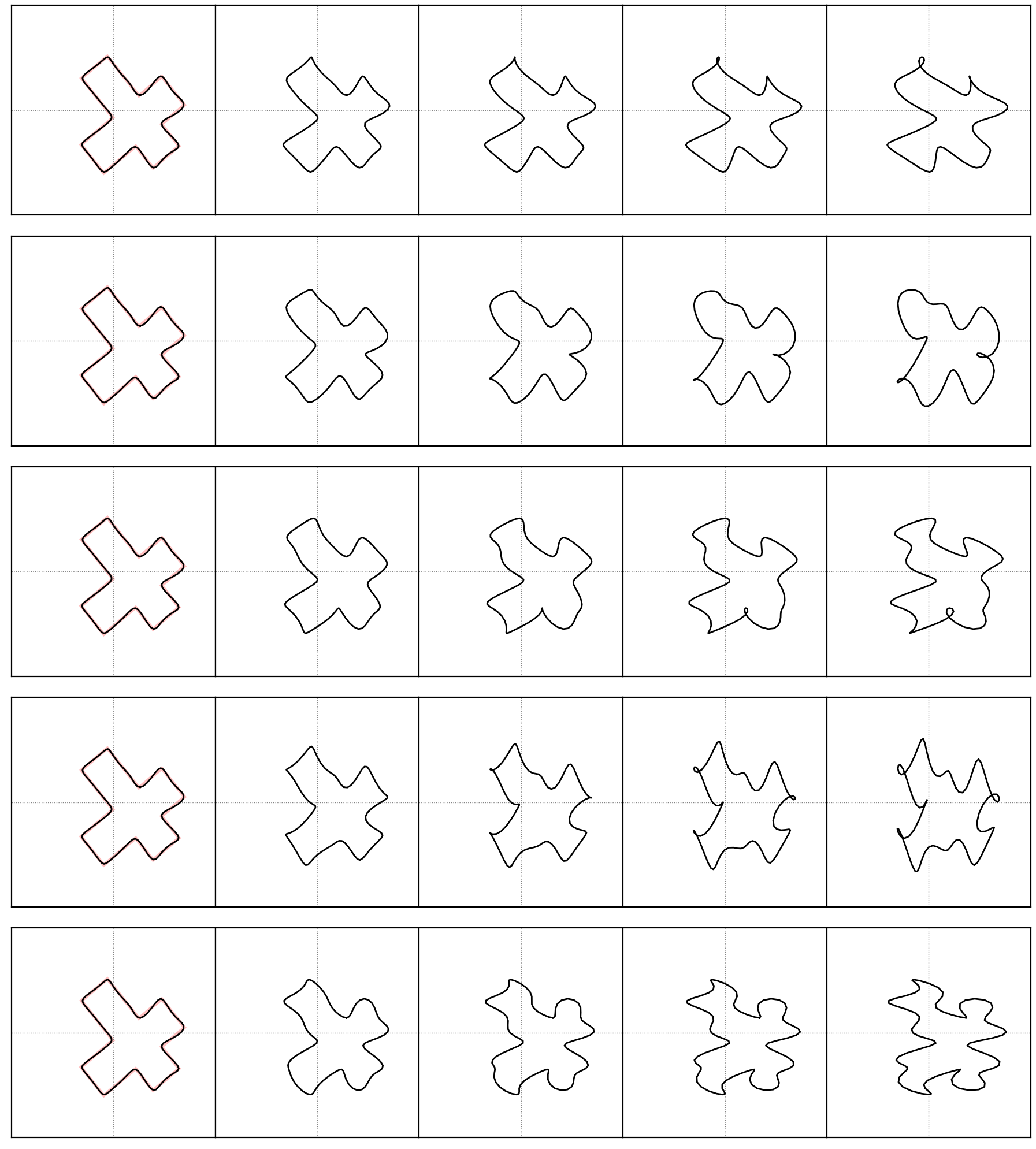
Figure 10: Samples from deeper Real-NVP models vs. ours, visualized in the same style as in the main paper.

Figure 11: Sensitivity of Fourier shapes to changes in a single parameter.

Details on Lens Shapes Data Set

The shapes in the Lens data set arise from the intersection of two circles. The first has a uniformly random radius $r$ within $[1,2]$, the second has exactly double that radius. They are positioned at a uniformly random angle, with their centers set apart by a distance of $2.4r$. Their intersection is centered at the origin and offset by a random distance from $\mathcal{N}(0,\tfrac{1}{2})$ in either dimension.

Details on Cross Shapes Data Set

The shapes for the larger Cross data set are generated by taking the union of two oblong rectangles crossing each other at a right angle. For both rectangles, the longer side length is drawn uniformly from $[\,3,5\,]$ and the other from $[\,\tfrac{1}{2},2\,]$. We shift both rectangles along their longer side by a uniformly random distance drawn from $[\,-\tfrac{3}{2},\tfrac{3}{2}\,]$.

Then we form the union and insert equally spaced points along the resulting polygon’s sides such that no line segment is longer than $\tfrac{1}{5}$. This is necessary to obtain dense point sequences which are approximated more faithfully by Fourier curves.

Finally, we center the shape at the origin, rotate it by a random angle and again shift it within the plane by a distance drawn from $\mathcal{N}(0,\tfrac{1}{2})$.

Training Hyper-Parameters

For all experiments, we used the Adam optimizer with betas $(0.9,0.95)$ for $50$ epochs with L2 weight regularization strength $1.86\cdot 10^{-5}$. Unless otherwise stated, we used exponential learning rate decay, starting at $0.01$ and ending at $0.0001$. We employ a hundredfold reduced learning rate for the first three epochs, as we find this helps set training of invertible networks on a stable track.

Where we use recursive coupling blocks, the number of neurons per hidden layer in the subnetworks is decreased by half with each level of recursion, down to a minimum of $1/8$ of the top level network size. Each subnetwork consists of two hidden layers and ReLU activations. Network parameters are initialized from a Gaussian distribution with $\sigma=0.005$.

UCI Data

For the Power data set, models were scaled to a budget of $5\cdot 10^{5}$ trainable parameters and we used a batch size of $1660$ (i.e. 1000 batches/epoch).

For the Gas data set, models were scaled to a budget of $5\cdot 10^{5}$ trainable parameters and we used a batch size of $853$ (i.e. 1000 batches/epoch).

For the Miniboone data set, models were scaled to a budget of $2.5\cdot 10^{5}$ trainable parameters and we used a batch size of $300$ (i.e. 100 batches/epoch).

Lens Shapes

We instantiate this data set with $10^{6}$ training and $10^{5}$ test samples and use a batch size of $10^{4}$. All unconditional models were scaled to a budget of $1\cdot 10^{5}$ trainable parameters, all conditional models to a budget of $4\cdot 10^{5}$.

Cross Shapes

We instantiate this data set with $10^{6}$ training and $10^{5}$ test samples and use a batch size of $10^{4}$. All unconditional models were scaled to a budget of $2\cdot 10^{6}$ trainable parameters, all conditional models to a budget of $4\cdot 10^{6}$. For some of the deeper models shown in the trade-off section later on (16 and 32 blocks), we initialize the learning rate to $0.001$ to stabilize training.

Shape Fitting Algorithm

In order to judge the quality of individual generated shapes, we compare to the best match among shapes from the ground truth distribution. This means we have to find the best match in an automated fashion. The way we do this differs slightly for the two types of shapes we used.

The algorithm for fitting a proper Lens shape $\hat{S}$ – parametrized by a tuple $\theta$ consisting of angle, scale and center – to a generated one $S$ works as follows:

1. find the two points $\mathbf{P}_{0},\mathbf{P}_{1}\in S$ which are furthest apart

2. $\alpha=\$ the angle of the line $\overrightarrow{\mathbf{P}_{0}\mathbf{P}_{1}}$

3. initialize shape parameters $\theta$ to $\bigl{(}\alpha,2,\tfrac{1}{n}\sum_{j=1}^{n}\mathbf{S}_{j}\bigr{)}$

4. use gradient descent to minimize $\mathcal{L}\bigl{(}\hat{S}(\theta),S\bigr{)}$, where

   $$\mathcal{L}\bigl{(}\hat{S}(\theta),S\bigr{)}=\frac{1}{m}\sum_{i=1}^{m}\min_{j}D_{ij}+\frac{1}{n}\sum_{j=1}^{n}\min_{i}D_{ij}$$

   $$\text{with }\mathbf{D}\in\mathbb{R}^{m\times n}\text{ and }D_{ij}=\|\mathbf{\hat{S}}_{i}-\mathbf{S}_{j}\|^{2}_{2}$$

5. repeat for initialization with angle $\alpha^{\prime}=\alpha+\pi$ (i.e. the “flipped” lens) and keep the result with lower $\mathcal{L}$

In other words, we minimize the average distance from each point in the fitted shape to the nearest point in the generated shape, and vice versa, starting from a strong heuristic guess for the correct angle. Since the angle has such a strong effect on the fit and our initial guess should be reasonably good, we set a lower learning rate for the angle parameter during gradient descent.

The equivalent procedure for the more complex Cross shapes data set requires a few changes to work well.

• The shape $\hat{S}$ is parameterized by a tuple $\theta$ consisting of width, length and lateral shift of each of the two bars, as well as an angle $\alpha$ and the center of their crossing.

• The initial angle $\alpha$ is taken from the dominant straight line within $S$, as determined by RANSAC (Fischler and Bolles 1981).

• A general clean Cross shape $\hat{S}$ is a twelve-sided polygon. We adapt the loss $\mathcal{L}$ from above by changing the first term to the average distance from each corner of the polygon $\hat{S}$ to the closest point in $S$, and the second term to the average distance from each point in $S$ to the closest line segment of $\hat{S}$.

• Because our Cross shapes can have very diverse layouts, initializations with wrong lateral shift often get stuck in a bad local minimum. To counteract this, we repeat the optimization for each of the nine archetypes shown in figure 9 and keep the result where $\mathcal{L}$ is lowest.

With these changes we consistently get a good fit $\hat{S}$, provided the generated $S$ actually resembles a Cross shape.

Samples from Deeper Models

In figure 11 we show qualitative results for deeper non-recursive models trained on the Cross shapes data set, all under identical training conditions and at the same total parameter budget of $2M$. Both visually and in terms of the $\mathbf{x}$ correlation matrix, recursive coupling with only 4 blocks is on par or better than non-recursive coupling with the same parameter budget spread across up to 32 blocks.

Sensitivity of the Fourier Curve Parameterization

To demonstrate how quickly Fourier shapes deteriorate as soon as a single parameter goes “out of sync”, we present figure 11. In each row, the same original shape is manipulated by adding an increasing offset ($0.1$ per column, left to right) to one arbitrary Fourier parameter $x_{i}$. It is clear that even minor mistakes in a single variable affect the entire shape. The quality of generated samples thus relies heavily on modelling correlations between the variables correctly.

Recursion Depth vs. Number of Blocks

We trained a number of models with varying recursion depth and number of blocks on the unconditional Cross data set to investigate the trade-off between these hyperparameters. The results are presented in tables 6, 7 and 8. A recursion depth of $0$ corresponds to standard Real-NVP coupling. Note that for the latter two tables, we lift the total parameter budget and instead only set a fixed size for the coupling networks within each single block.

We find that in all cases, the best results both statistically and in terms of shape quality are achieved by networks with one or two levels of recursion. Beyond that, the advantages of recursive coupling start to be outweighed by the parameter trade-off or the challenges of training more complex networks. We also find that the deeper networks (i.e. 16 and 32 blocks) exhibit less stable training results, which we consider an argument in favor of using fewer, more expressive coupling blocks.

Proof of Concept:
Bayesian filtering using HINT

In the following, we compare HINT and a conditional adaptation of Real-NVP (Ardizzone et al. (2019a), called INN for short) on a Bayesian filtering test case. Filtering is a recursive Bayesian estimation task on hidden Markov models which requires to estimate the posterior of unobserved variables. The posterior is then used as a prior for the next step, and subsequently updated by newly arriving observations. Standard sampling algorithms for filtering require a Monte Carlo approximation of the analytic expression of the prior, which may dramatically deteriorate performance due to large variance. HINT, on the other hand, does not need a functional form of the prior but only samples from it, which makes it an interesting candidate method for filtering.

As a task, we use the general predator-prey model, also termed competitive Lotka-Volterra equations, which typically describes the interaction of $d$ species in a biological system over time:

$$\frac{\partial}{\partial t}{x_{i}} =\beta_{i}x_{i}\left(1-\sum_{j=1}^{d}\alpha_{ij}x_{j}\right)$$ (13)

The undisturbed growth rate of species $i$ is given by $\beta_{i}$ (can be $<$ or $>0$, growing or shrinking naturally), and is further affected by the other species in a positive way ($\alpha_{ij}>0$, predator), or in a negative way ($\alpha_{ij}<0$, prey). The solutions to this system of equations can not be expressed analytically, which makes their prediction a challenging task. Additionally, we make the process stochastic, by adding random noise at each time step. Therefore, at each time step, noisy measurements of $x_{1},x_{2},x_{3}$ are observed, with the task to predict the remaining population $x_{4}$, given the current and past observations.

We compare this to an implementation using a standard coupling block INN with the training procedure proposed by Ardizzone et al. (2019a). The results for a single example time-series are shown in figure 12. We find that the standard INN does not make meaningful predictions in the short- or mid-term, only correctly predicting the final dying off of population $x_{4}$. HINT on the other hand is able to correctly model the entire sequence. Importantly, the modeled posterior distribution at each step correctly contracts over time, as more measurements are accumulated. The experimental details are as follows:

Figure 12: Contracting posterior for sequential Lotka-Volterra.

Figure 13: Population development in competitive Lotka-Volterra model. $x_{1}$, $x_{2}$ and $x_{3}$ are only accessible via noisy measurements (small crosses), the colored bands show the standard deviation of this noise. The task is to predict $x_{4}$ as the sequence develops.

Parameters $\bm{\alpha}$ and $\bm{\beta}$ for the 4d competitive Lotka-Volterra model in equation 13 were picked randomly as

$$\bm{\beta} =\scalebox{0.9}{$\begin{bmatrix}1.14143055\\ 0.64270729\\ 1.42981209\\ 0.90620443\end{bmatrix}$}\;\text{and}$$

$$\bm{\alpha} =\scalebox{0.9}{$\begin{bmatrix}0.78382338&1.26614888&1.25787652&0.80904295\\ 1.00470891&0.32719451&1.34501072&1.29758381\\ 1.28599724&0.39362355&0.89977679&1.00063551\\ 1.12163602&1.08672758&1.39634746&0.53592833\end{bmatrix}$},$$

and the true initial population values $$\mathbf{x}_{0}^{\ast}$$ set to

$$\mathbf{x}_{0}^{\ast} =\scalebox{0.9}{$\begin{bmatrix}1.00471435\\ 0.98809024\\ 1.01432707\\ 0.99687348\end{bmatrix}$}.$$

Figure 13 shows the resulting development of the four populations over ten unit time steps, including noise on the observed values for $x_{1}$, $x_{2}$ and $x_{3}$.

Both the INN and the HINT network we trained consist of ten (non-recursive) coupling blocks with a total of $10^{6}$ trainable weights. We used Adam to train both for $50$ epochs per time step with $64000$ training samples and a batch size of $500$. The learning rate started at $10^{\sminus 2}$ and exponentially decayed to $10^{\sminus 3}$ (HINT) and $10^{\sminus 4}$ (INN), respectively. Inference on $x_{4}$ begins with an initial guess at $t=0$ drawn from $\mathcal{N}(1,\tfrac{1}{10})$.

Table 6: Comparing the effect of more coupling blocks versus more levels of recursion within the blocks, while keeping the network parameter budget fixed at $2\cdot 10^{6}$.

Recursion depth		0	1	2	3
4 blocks	LL $\uparrow$	$3.419$	$3.680$	$3.663$	$3.666$
	IoU $\uparrow$	$0.314$	$0.857$	$0.823$	$0.835$
	H-dist $\downarrow$	$0.236$	$0.066$	$0.077$	$0.071$
	Corr $\downarrow$	$0.0454$	$0.0022$	$0.0027$	$0.0026$
8 blocks	LL $\uparrow$	$3.329$	$3.592$	$3.593$
	IoU $\uparrow$	$0.588$	$0.802$	$0.817$
	H-dist $\downarrow$	$0.138$	$0.085$	$0.083$
	Corr $\downarrow$	$0.0064$	$0.0030$	$0.0028$
16 blocks	LL $\uparrow$	$3.530$	$3.623$
	IoU $\uparrow$	$0.778$	$0.841$
	H-dist $\downarrow$	$0.101$	$0.073$
	Corr $\downarrow$	$0.0035$	$0.0026$
32 blocks	LL $\uparrow$	$3.578$
	IoU $\uparrow$	$0.836$
	H-dist $\downarrow$	$0.082$
	Corr $\downarrow$	$0.0029$

Table 7: Comparing the effect of more coupling blocks versus more levels of recursion within the blocks, while affording internal networks a width of $128$ neurons, halved at every recursion level.

Recursion depth		0	1	2	3
4 blocks	LL $\uparrow$	$3.496$	$3.595$	$3.612$	$3.614$
	IoU $\uparrow$	$0.713$	$0.806$	$0.813$	$0.804$
	H-dist $\downarrow$	$0.115$	$0.090$	$0.085$	$0.082$
	Corr $\downarrow$	$0.0032$	$0.0025$	$0.0024$	$0.0023$
8 blocks	LL $\uparrow$	$3.623$	$3.664$	$3.651$
	IoU $\uparrow$	$0.822$	$0.864$	$0.860$
	H-dist $\downarrow$	$0.081$	$0.065$	$0.067$
	Corr $\downarrow$	$0.0023$	$0.0018$	$0.0018$
16 blocks	LL $\uparrow$	$3.631$	$3.613$
	IoU $\uparrow$	$0.839$	$0.819$
	H-dist $\downarrow$	$0.074$	$0.080$
	Corr $\downarrow$	$0.0020$	$0.0022$
32 blocks	LL $\uparrow$	$3.612$
	IoU $\uparrow$	$0.814$
	H-dist $\downarrow$	$0.086$
	Corr $\downarrow$	$0.7490$

Table 8: Comparing the effect of more coupling blocks versus more levels of recursion within the blocks, while affording internal networks a width of $512$ neurons, halved at every recursion level.

Recursion depth		0	1	2	3
4 blocks	LL $\uparrow$	$3.620$	$3.685$	$3.685$	$3.681$
	IoU $\uparrow$	$0.846$	$0.837$	$0.825$	$0.810$
	H-dist $\downarrow$	$0.082$	$0.069$	$0.068$	$0.071$
	Corr $\downarrow$	$0.0023$	$0.0025$	$0.0023$	$0.0025$
8 blocks	LL $\uparrow$	$3.669$	$3.716$	$3.722$
	IoU $\uparrow$	$0.863$	$0.883$	$0.888$
	H-dist $\downarrow$	$0.064$	$0.053$	$0.052$
	Corr $\downarrow$	$0.0020$	$0.0018$	$0.0017$
16 blocks	LL $\uparrow$	$3.702$	$3.685$
	IoU $\uparrow$	$0.882$	$0.878$
	H-dist $\downarrow$	$0.055$	$0.060$
	Corr $\downarrow$	$0.0017$	$0.0017$
32 blocks	LL $\uparrow$	$3.654$
	IoU $\uparrow$	$0.813$
	H-dist $\downarrow$	$0.072$
	Corr $\downarrow$	$0.0021$

References

- Ardizzone et al. (2019a) Ardizzone, L.; Kruse, J.; Rother, C.; and Köthe, U. 2019a. Analyzing inverse problems with invertible neural networks. In Intl. Conf. Learning Representations.
- Ardizzone et al. (2019b) Ardizzone, L.; Lüth, C.; Kruse, J.; Rother, C.; and Köthe, U. 2019b. Guided image generation with conditional invertible neural networks. arXiv:1907.02392 .
- Behrmann et al. (2019) Behrmann, J.; Grathwohl, W.; Chen, R. T. Q.; Duvenaud, D.; and Jacobsen, J.-H. 2019. Invertible residual networks. In Intl. Conf. Machine Learning.
- Chen et al. (2019) Chen, T. Q.; Behrmann, J.; Duvenaud, D. K.; and Jacobsen, J.-H. 2019. Residual flows for invertible generative modeling. In Adv. Neural Information Process. Syst., 9913–9923.
- Csilléry et al. (2010) Csilléry, K.; Blum, M.; Gaggiotti, O.; and François, O. 2010. Approximate Bayesian Computation (ABC) in practice. Trends in Ecology & Evolution 25: 410–8. doi:10.1016/j.tree.2010.04.001.
- Detommaso et al. (2019) Detommaso, G.; Kruse, J.; Ardizzone, L.; Rother, C.; Köthe, U.; and Scheichl, R. 2019. HINT: Hierarchical Invertible Neural Transport for general and sequential Bayesian inference. arXiv:1905.10687v1 .
- Dinh, Krueger, and Bengio (2015) Dinh, L.; Krueger, D.; and Bengio, Y. 2015. NICE: Non-linear Independent Components Estimation. In Intl. Conf. Learning Representations.
- Dinh, Sohl-Dickstein, and Bengio (2017) Dinh, L.; Sohl-Dickstein, J.; and Bengio, S. 2017. Density estimation using Real NVP. In Intl. Conf. Learning Representations.
- Dolgov et al. (2020) Dolgov, S.; Anaya-Izquierdo, K.; Fox, C.; and Scheichl, R. 2020. Approximation and sampling of multivariate probability distributions in the tensor train decomposition. Stat. Comput. 30: 603–625.
- Dua and Graff (2017) Dua, D.; and Graff, C. 2017. UCI Machine Learning Repository. URL http://archive.ics.uci.edu/ml. Last accessed on 2021-03-08.
- Durkan et al. (2019) Durkan, C.; Bekasov, A.; Murray, I.; and Papamakarios, G. 2019. Neural spline flows. In Adv. Neural Information Processing Systems, 7509–7520.
- Fischler and Bolles (1981) Fischler, M. A.; and Bolles, R. C. 1981. Random Sample Consensus: A Paradigm for Model Fitting with Applications to Image Analysis and Automated Cartography. Commun. ACM 24(6): 381–395. ISSN 0001-0782. doi:10.1145/358669.358692. URL https://doi.org/10.1145/358669.358692.
- Gomez et al. (2017) Gomez, A. N.; Ren, M.; Urtasun, R.; and Grosse, R. B. 2017. The reversible residual network: Backpropagation without storing activations. In Adv. Neural Information Processing Systems, 2214–2224.
- Grathwohl et al. (2019) Grathwohl, W.; Chen, R. T. Q.; Bettencourt, J.; and Duvenaud, D. 2019. Scalable reversible generative models with free-form continuous dynamics. In Intl. Conf. Learning Representations.
- Gretton et al. (2012) Gretton, A.; Borgwardt, K. M.; Rasch, M. J.; Schölkopf, B.; and Smola, A. 2012. A kernel two-sample test. J. Mach. Learn. Res. 13(Mar): 723–773.
- Huang et al. (2018) Huang, C.-W.; Krueger, D.; Lacoste, A.; and Courville, A. 2018. Neural autoregressive flows. In Intl. Conf. Machine Learning, 2078–2087.
- Hyvärinen and Pajunen (1999) Hyvärinen, A.; and Pajunen, P. 1999. Nonlinear independent component analysis: Existence and uniqueness results. Neural Networks 12(3): 429–439.
- Jaini, Selby, and Yu (2019) Jaini, P.; Selby, K. A.; and Yu, Y. 2019. Sum-of-squares polynomial flow. In Intl. Conf. Machine Learn., 3009–3018.
- Karami et al. (2019) Karami, M.; Schuurmans, D.; Sohl-Dickstein, J.; Dinh, L.; and Duckworth, D. 2019. Invertible Convolutional Flow. In Adv. Neural Information Processing Systems, 5636–5646.
- Kingma and Dhariwal (2018) Kingma, D. P.; and Dhariwal, P. 2018. Glow: Generative flow with invertible 1x1 convolutions. arXiv:1807.03039 .
- Kingma et al. (2016) Kingma, D. P.; Salimans, T.; Jozefowicz, R.; Chen, X.; Sutskever, I.; and Welling, M. 2016. Improved variational inference with inverse autoregressive flow. In Adv. Neural Information Processing Systems, 4743–4751.
- Kobyzev, Prince, and Brubaker (2019) Kobyzev, I.; Prince, S.; and Brubaker, M. A. 2019. Normalizing flows: An introduction and review of current methods. arXiv:1908.09257 .
- Kruse et al. (2019) Kruse, J.; Ardizzone, L.; Rother, C.; and Köthe, U. 2019. Benchmarking invertible architectures on inverse problems. ICML Workshop on Invertible Neural Nets and Normalizing Flows (INNF’19) .
- Liao, He, and Shu (2019) Liao, H.; He, J.; and Shu, K. 2019. Generative model With dynamic linear flow. IEEE Access 7: 150175–150183. ISSN 2169-3536. doi:10.1109/ACCESS.2019.2947567.
- Liu and Wang (2016) Liu, Q.; and Wang, D. 2016. Stein variational gradient descent: A general purpose Bayesian inference algorithm. In Adv. Neural Information Processing Systems, 2378–2386.
- Ma et al. (2019) Ma, X.; Kong, X.; Zhang, S.; and Hovy, E. 2019. MaCow: Masked convolutional generative flow. Adv. Neural Information Processing Systems 5891–5900.
- Marzouk et al. (2016) Marzouk, Y.; Moselhy, T.; Parno, M.; and Spantini, A. 2016. Sampling via measure transport: An introduction. In Ghanem, R.; Higdon, D.; and Owhadi, H., eds., Handbook of Uncertainty Quantification, 1–41. Springer.
- McGarva and Mullineux (1993) McGarva, J.; and Mullineux, G. 1993. Harmonic representation of closed curves. Appl. Math. Model. 17(4): 213–218.
- Papamakarios et al. (2019) Papamakarios, G.; Nalisnick, E.; Rezende, D. J.; Mohamed, S.; and Lakshminarayanan, B. 2019. Normalizing flows for probabilistic modeling and inference. arXiv:1912.02762 .
- Papamakarios, Pavlakou, and Murray (2017) Papamakarios, G.; Pavlakou, T.; and Murray, I. 2017. Masked autoregressive flow for density estimation. In Adv. Neural Information Processing Systems, 2338–2347.
- Rezende and Mohamed (2015) Rezende, D.; and Mohamed, S. 2015. Variational inference with normalizing flows. In Intl. Conf. Machine Learning, 1530–1538.
- Song, Meng, and Ermon (2019) Song, Y.; Meng, C.; and Ermon, S. 2019. MintNet: Building invertible neural networks with masked convolutions. In Adv. Neural Information Processing Systems, 11002–11012.
- Stoer and Bulirsch (2013) Stoer, J.; and Bulirsch, R. 2013. Introduction to Numerical Analysis, volume 12. Springer Science & Business Media.
- Van den Oord et al. (2016) Van den Oord, A.; Kalchbrenner, N.; Espeholt, L.; Vinyals, O.; Graves, A.; et al. 2016. Conditional image generation with PixelCNN decoders. In Adv. Neural Information Processing Systems, 4790–4798.
- Van den Oord, Kalchbrenner, and Kavukcuoglu (2016) Van den Oord, A.; Kalchbrenner, N.; and Kavukcuoglu, K. 2016. Pixel recurrent neural networks. In Intl. Conf. Machine Learning, 1747–1756.
- Villani (2008) Villani, C. 2008. Optimal Transport: Old and New, volume 338. Springer Science & Business Media.
- Winkler et al. (2019) Winkler, C.; Worrall, D.; Hoogeboom, E.; and Welling, M. 2019. Learning likelihoods with conditional normalizing flows. arXiv:1912.00042 .