DIANet: Dense-and-Implicit Attention Network

Abstract

Attention networks have successfully boosted the performance in various vision problems. Previous works lay emphasis on designing a new attention module and individually plug them into the networks. Our paper proposes a novel-and-simple framework that shares an attention module throughout different network layers to encourage the integration of layer-wise information and this parameter-sharing module is referred as Dense-and-Implicit-Attention (DIA) unit. Many choices of modules can be used in the DIA unit. Since Long Short Term Memory (LSTM) has a capacity of capturing long-distance dependency, we focus on the case when the DIA unit is the modified LSTM (refer as DIA-LSTM). Experiments on benchmark datasets show that the DIA-LSTM unit is capable of emphasizing layer-wise feature interrelation and leads to significant improvement of image classification accuracy. We further empirically show that the DIA-LSTM has a strong regularization ability on stabilizing the training of deep networks by the experiments with the removal of skip connections or Batch Normalization (?) in the whole residual network.

Introduction

Attention, a cognitive process that selectively focuses on a small part of information while neglects other perceivable information (?), has been used to effectively ease neural networks from learning large information contexts from sentences (?; ?; ?), images (?; ?) and videos (?). Especially in computer vision, deep neural networks (DNNs) incorporated with special operators that mimic the attention mechanism can process informative regions in an image efficiently. These operators are modularized and plugged into networks as attention modules (?; ?; ?; ?; ?; ?).

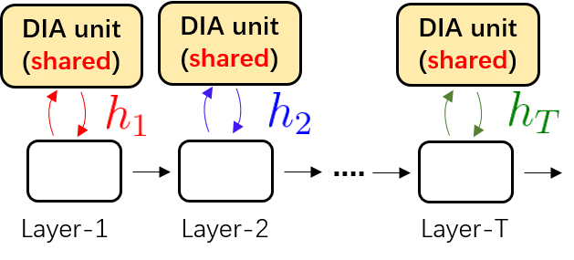
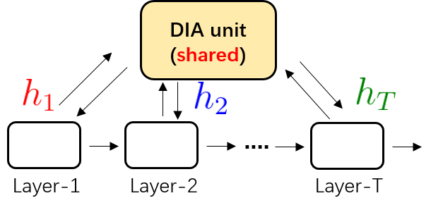
Figure 1: Left: explicit structure of DIANet. Right: implicit connection of DIA unit.

Previous works lay emphasis on designing a new attention module and individually plug them into networks. Generally, the attention module can be divided into three parts: extraction, processing and recalibration. First, the added plug-in module extracts internal features of a network which can be squeezed channel-wise information (?; ?) or spatial information (?; ?; ?). Next, the module processes the extraction and generates a mask to measure the importance of the features via fully connected layer (?), convolution layer (?). Last, the mask is applied to recalibrate the features. Previous works focus on designing effective ways to process the extracted features. There is one obvious common ground where the attention modules are individually plugged into each layer throughout DNNs (?; ?; ?; ?).

Our Framework. Differently, we proposes a novel-and-simple framework that shares an attention module throughout different network layers to encourage the integration of layer-wise information and this parameter-sharing module is referred as Dense-and-Implicit-Attention (DIA) unit. The structure and computation flow of a DIA unit is visualized in Figure 2. There are also three parts: extraction (\tiny{1}⃝), processing (\tiny{2}⃝) and recalibration (\tiny{3}⃝) in the DIA unit. The \tiny{2}⃝ is the main module in the DIA unit to model network attention and is the key innovation of the proposed method where the parameters of the attention module is shared.

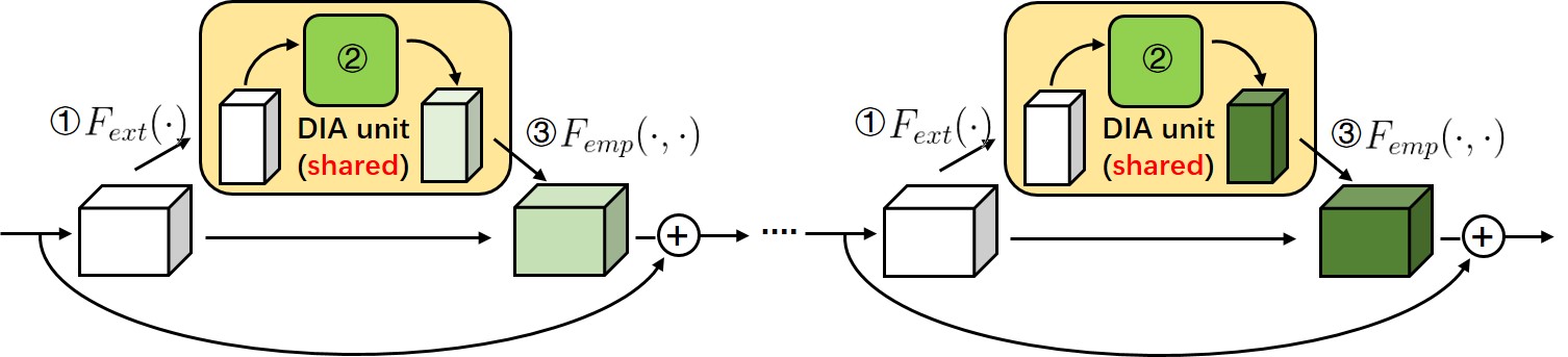
Figure 2: DIA units. $F_{ext}$ means the operation for extracting different scales of features. $F_{emp}$ means the operation for emphasizing features.

Characteristics and Advantages. (1) As shown in Figure 2, the DIA unit is placed parallel to the network backbone, and it is shared with all the layers in the same stage (the collection of successive layers with same spatial size, as defined in (?)) to improve the interaction of layers at different depth. (2) As the DIA unit is shared, the number of parameter increment from the DIA unit remains roughly constant as the depth of the network increases.

We show the feasibility of our framework by applying SE module (?) in DIA unit. SE module, a representative of attention mechanism, is used for each block individually in its original design. In our framework, we share the same SE module (refer as DIA-SE) throughout all layers in the same stage. It is easy to see that DIA-SE has the same computation cost as SE, but in Table 1, DIA-SE has better generalization and smaller parameter increment.

model	#P (M)	top1-acc.
Org	1.73	73.43(±0.43)
SE	1.93	75.03(±0.33)
DIA-SE	1.74	75.74(±0.41)

Table 1: Testing accuracy (mean $\pm$ std%) on CIFAR100 and ResNet164 with different attention modules. ”Org” means the original backbone of ResNet164. #P (M) means the number of parameters (million).

Implicit and Dense Connection. We illustrate how the DIA unit connects all layers in the same stage implicitly and densely. Consider a stage consisting many layers in Figure 1 (Left). It is an explicit structure with a DIA unit and one layer seems not to connect the other layers except the network backbone. In fact, the different layers use the parameter-sharing attention module and the layer-wise information jointly influences the update of learnable parameters in the module, which causes implicit connections between layers with the help of the shared DIA unit as in Figure 1 (Right). Since there is communication between every pair of layers, the connections over all layers are dense.

DIA-LSTM

The idea of parameter sharing also used in Recurrent Neural Network (RNN) to capture contextual information so we consider apply RNN in our framework to model the layer-wise interrelation. Since Long Short Term Memory (LSTM) (?) is capable of capturing long-distance dependency, we mainly focus on the case when we use LSTM in DIA unit (DIA-LSTM) and the remainder of our paper studies DIA-LSTM.

Figure 3 is the showcase of DIA-LSTM. A global average pooling (GAP) layer (as the \tiny{1}⃝ in Figure 2) is used to extract global information from current layer. A LSTM module (as the \tiny{2}⃝ in Figure 2) is used to integrate multi-scale information and there are three inputs passed to the LSTM: the extracted global information from current raw feature map, the hidden state vector $h_{t-1}$, and cell state vector $c_{t-1}$ from previous layers. Then the LSTM outputs the new hidden state vector $h_{t}$ and the new cell state vector $c_{t}$. The cell state vector $c_{t}$ stores the information from the $t^{th}$ layer and its preceding layers. The new hidden state vector $h_{t}$ (dubbed as attention vector in our work) is then applied back to the raw feature map by channel-wise multiplication (as the \tiny{3}⃝ in Figure 2) to recalibrate the feature.

The LSTM in the DIA unit plays a role to bridge the current layer and preceding layers such that the DIA unit can adaptively learn the non-linearity relationship between features in two different dimensions. The first dimension of features is the internal information of the current layer. The second dimension represents the outer information, regarded as layer-wise information, from the preceding layers. The non-linearity relationship between these two dimensions will benefit attention modeling for the current layer. The multiple dimension modeling enables DIA-LSTM to have regularization effect.

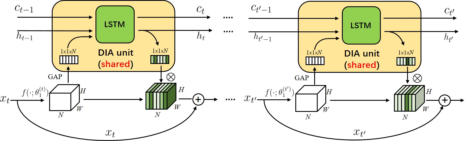
Figure 3: The showcase of DIA-LSTM. In the LSTM cell, $c_{t}$ is the cell state vector and $h_{t}$ is the hidden state vector. GAP means global average pool over channels and $\otimes$ means channel-wise multiplication.

Our contribution

We summary our contribution as followed,

1. We proposes a novel-and-simple framework that shares an attention module throughout different network layers to encourage the integration of layer-wise information.

2. We propose incorporating LSTM in DIA unit (DIA-LSTM) and show the effectiveness of DIA-LSTM for image classification by conducting experiments on benchmark datasets and popular networks.

Related Works

Attention Mechanism in Computer Vision. (?; ?) use attention mechanism in image classification via utilizing a recurrent neural network to select and process local regions at high resolution sequentially. Concurrent attention-based methods tend to construct operation modules to capture non-local information in an image (?; ?), and model the interrelationship between channel-wise features (?; ?). The combination of multi-level attentions are also widely studied (?; ?; ?; ?). Prior works (?; ?; ?; ?; ?; ?; ?) usually insert an attention module in each layer individually. In this work, the DIA unit is innovatively shared for all the layers in the same stage of the network, and the existing attention modules can be composited into the DIA unit readily. Besides, we adopt a global average pooling in part \tiny{1}⃝ to extract global information and a channel-wise multiplication in part \tiny{3}⃝ to recalibrate features, which is similar to SENet (?).

Dense Network Topology. DenseNet proposed in (?) connects all pairs of layers directly with an identity map. Through reusing features, DenseNet has the advantage of higher parameter efficiency, the better capacity of generalization, and more accessible training than alternative architectures (?; ?; ?). Instead of explicitly dense connections, the DIA unit implicitly links layers at different depth via a shared module and leads to dense connection.

Multi-Dimension Feature Integration. (?) experimentally analyzes that even the simple aggregation of low-level visual features sampled from wide inception field can be efficient and robust for context representation, which inspires (?; ?) to incorporate multi-level features to improve the network representation. (?) also demonstrates that by biasing the feature response in each convolutional layers using different activation functions, the deeper layer could achieve the better capacity of capturing the abstract pattern in DNN. In DIA unit, the high non-linearity relationship between multi-dimension features are learned and integrated via the LSTM module.

Dense-and-Implicit Attention Network

In this section, we will formally introduce the DIA-LSTM unit. We use the modified LSTM module in the DIA unit. Afterwards, a DIANet is referred to a network built with DIA-LSTM units.

Formulation of DIA-LSTM unit

As shown in Figure 3 when a DIA-LSTM unit is built with a residual network (?), the input of the $t^{th}$ layer is $x_{t}\in\mathbb{R}^{W\times H\times N}$, where $W,H$ and $N$ mean width, height and the number of channels, respectively. $f(\cdot;\theta_{1}^{(t)})$ is the residual mapping at the $t^{th}$ layer with parameters $\theta_{1}^{(t)}$ as introduced in (?). Let $a_{t}=f(x_{t};\theta_{1}^{(t)})\in\mathbb{R}^{W\times H\times N}.$ Next, a global average pooling denoted as $\text{GAP}(\cdot)$ is applied to $a_{t}$ to extract global information from features in the current layer. Then $\text{GAP}(a_{t})\in\mathbb{R}^{N}$ is passed to LSTM along with a hidden state vector $h_{t-1}$ and a cell state vector $c_{t-1}$ ( $h_{0}$ and $c_{0}$ are initialized as zero vectors). The LSTM finally generates a current hidden state vector $h_{t}\in\mathbb{R}^{N}$ and a cell state vector $c_{t}\in\mathbb{R}^{N}$ as

$$(h_{t},c_{t})=\text{LSTM}(\text{GAP}(a_{t}),h_{t-1},c_{t-1};\theta_{2}).$$ (1)

In our model, the hidden state vector $h_{t}$ is regarded as attention vector to adaptively recalibrate feature maps. We apply channel-wise multiplication $\otimes$ to enhance the importance of features, i.e., $a_{t}\otimes h_{t}$ and obtain $x_{t+1}$ after skip connection, i.e., $x_{t+1}=x_{t}+a_{t}\otimes h_{t}$. Table 2 shows the formulation of ResNet, SENet, and DIANet, and Part (b) is the main difference between them. The LSTM module is used repeatedly and shared with different layers in parallel to the network backbone. Therefore the number of parameters $\theta_{2}$ in a LSTM does not depend on the number of layers in the backbone, e.g., $t$. SENet utilizes a attention-module consisted of fully connected layers to model the channel-wise dependency for each layer individually (?). The total number of parameters brought by the add-in modules depends on the number of layers in the backbone and increases with the number of layers.

	ResNet	SENet	DIANet (ours)
(a)	$a_{t}=f(x_{t};\theta_{1}^{(t)})$	$a_{t}=f(x_{t};\theta_{1}^{(t)})$	$a_{t}=f(x_{t};\theta_{1}^{(t)})$
(b)	-	$h_{t}=\text{FC}(\text{GAP}(a_{t});\theta_{2}^{(t)})$	$(h_{t},c_{t})=\text{LSTM}(\text{GAP}(a_{t}),h_{t-1},c_{t-1};\theta_{2})$
(c)	$x_{t+1}=x_{t}+a_{t}$	$x_{t+1}=x_{t}+a_{t}\otimes h_{t}$	$x_{t+1}=x_{t}+a_{t}\otimes h_{t}$

Table 2: Formulation for the structure of ResNet, SENet, and DIANet. $f$ is the convolution layer. FC means fully connected layer and GAP indicates global average pooling.

Modified LSTM Module

Now we introduce the modified LSTM module used in Figure 3. The design of attention module usually requires the value of the attention vector in range $[0,1]$ and also requires small parameter increment. We conducts some modifications in LSTM module used in DIA-LSTM. As shown in Figure 4, compared to the standard LSTM (?) module, there are two modifications in our purposed LSTM: 1) a shared linear transformation to reduce input dimension of LSTM; 2) a careful selected activation function for better performance.

(1) Parameter Reduction. A standard LSTM consists of four linear transformation layers as shown in Figure 4 (Left). Since $y_{t}$, $h_{t-1}$ and $h_{t}$ are of the same dimension $N$, the standard LSTM may cause $8N^{2}$ parameter increment as shown in Appendix. When the number of channels is large, e.g., $N=2^{10}$, the parameter increment of added-in LSTM module in the DIA unit will be over 8 million, which can hardly be tolerated.

As shown in Figure 4 (Top), $h_{t-1}$ and $y_{t}$ are passed to four linear transformation layers with the same input and output dimension $N$. In the DIA-LSTM, a linear transformation layer (denoted as “Linear1” in Figure 4 (Bottom)) with a smaller output dimension are applied to $h_{t-1}$ and $y_{t}$. We use reduction ratio $r$ in the Linear1. Specifically, we reduce the dimension of the input from $1\times 1\times N$ to $1\times 1\times N/r$ and then apply the ReLU activation function to increase non-linearity in this module. The dimension of the output from ReLU function are changed back to $1\times 1\times N$ when the output is passed to those four linear transformation functions. This modification can enhance the relationship between the inputs for different parts in DIA-LSTM and also effectively reduce the number of parameters by sharing a linear transformation for dimension reduction. The number of parameter increment reduces from $8N^{2}$ to $10N^{2}/r$ as shown in the Appendix, and we find that when we choose an appropriate reduction ratio $r$, we can make a better trade-off between parameter reduction and the performance of DIANet. Further experimental results will be discussed in the ablation study later.

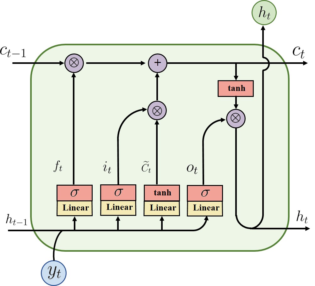
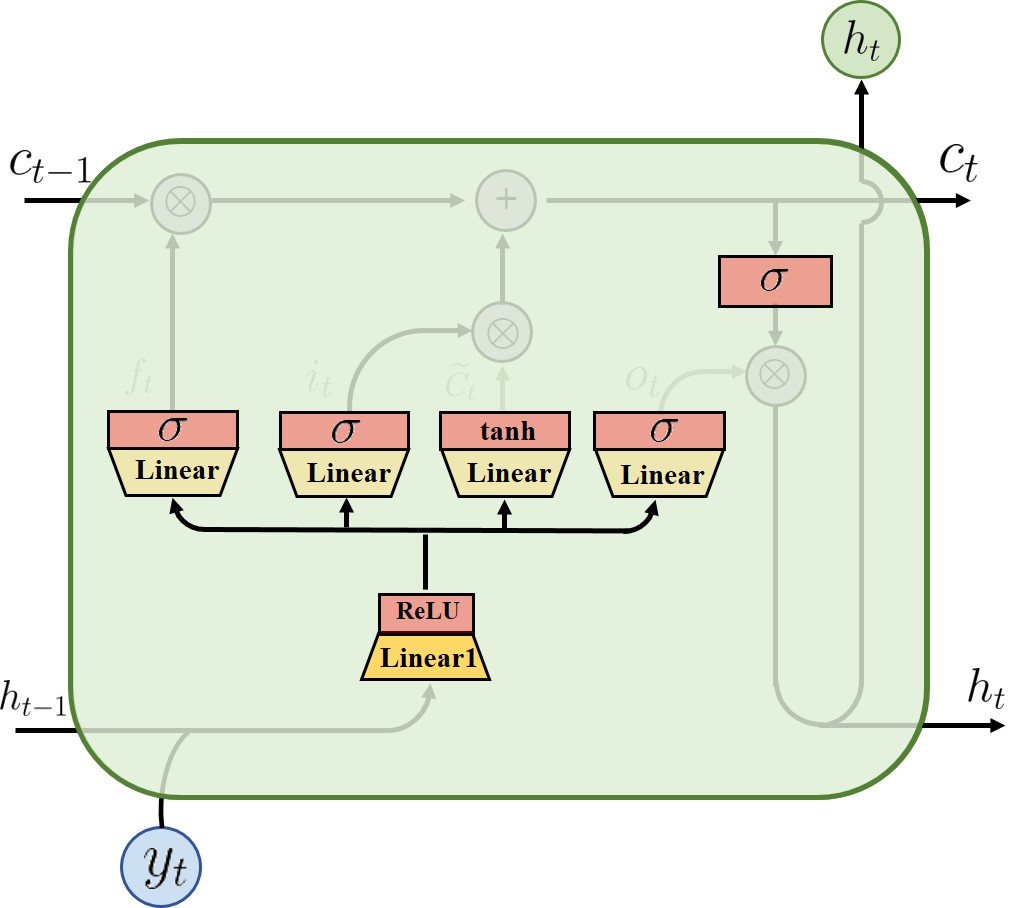
Figure 4: Top. The standard LSTM cell. Bottom. The modified LSTM cell in DIA-LSTM unit. We highlight the modified component in the modified LSTM. “$\sigma$” means the sigmoid activation. “Linear” means the linear transformation.

(2) Activation Function. Sigmoid function ($\sigma(z)=1/(1+e^{-z})$) is used in many attention-based methods like SENet (?), CBAM (?) to generate attention maps as a gate mechanism. As shown in Figure 4 (Bottom), we change the activation function of the output layer from Tanh to Sigmoid. Further discussion will be presented in ablation study.

Experiments

In this section, we evaluate the performance of the DIA-LSTM unit in image classification task and empirically demonstrate its effectiveness. We conduct experiments on popular networks for benchmark datasets. Since SENet (?) is also a channel-specific attention model, we compare DIANet with SENet. For a fair comparison, we adjust the reduction ratio such that the number of parameters of DIANet is similar to that of SENet.

Dataset and Model. We conduct experiments on CIFAR10, CIFAR100 (?), and ImageNet 2012 (?) using ResNet (?), PreResNet (?), WRN (?) and ResNeXt (?). CIAFR10 or CIFAR100 has 50k train images and 10k test images of size 32 by 32, but has 10 and 100 classes respectively. ImageNet 2012 (?) comprises 1.28 million training and 50k validation images from 1000 classes, and the random cropping of size 224 by 224 is used in our experiments. The details can be found in Appendix.

Image Classification. As shown in Table 3, DIANet improves the testing accuracy significantly over the original networks and consistently comparing with SENet for different datasets. In particular, the performance improvement of the ResNet with the DIA unit is most remarkable. Due to the popularity of ResNet, the DIA unit may be applied in other computer vision tasks.

	Dataset	original		SENet		DIANet
		$\#$P(M)	top1-acc.	$\#$P(M)	top1-acc.	$\#$P(M)	top1-acc.	$r$
ResNet164	CIFAR100	1.73	73.43	1.93	75.03	1.95	76.67	4
PreResNet164	CIFAR100	1.73	76.53	1.92	77.41	1.96	78.20	4
WRN52-4	CIFAR100	12.07	79.75	12.42	80.35	12.30	80.99	4
ResNext101,8x32	CIFAR100	32.14	81.18	34.03	82.45	33.01	82.46	4
ResNet164	CIFAR10	1.70	93.54	1.91	94.27	1.92	94.58	4
PreResNet164	CIFAR10	1.70	95.01	1.90	95.18	1.94	95.23	4
WRN52-4	CIFAR10	12.05	95.96	12.40	95.95	12.28	96.17	4
ResNext101,8x32	CIFAR10	32.09	95.73	33.98	96.09	32.96	96.24	4
ResNet34	ImageNet	21.81	73.93	21.97	74.39	21.98	74.60	20
ResNet50	ImageNet	25.58	76.01	28.09	76.61	28.38	77.24	20
ResNet152	ImageNet	60.27	77.58	66.82	78.36	65.85	78.87	10
ResNext50,32x4	ImageNet	25.03	77.19	27.56	78.04	27.83	78.32	20

Table 3: Testing accuracy (%) on CIFAR10, CIFAR100 and ImageNet 2012. “$\#$P(M)” means the number of parameters (million). The rightmost “$r$” indicates the reduction ratio of DIANet.

Ablation Study

In this section, we conduct ablation experiments to explore how to better embed DIA-LSTM units in different neural network structures and gain a deeper understanding of the role of components in the unit. All experiments are performed on CIFAR100 with ResNet. For simplicity, DIANet164 is denoted as a 164-layer ResNet built with DIA-LSTM units.

Reduction ratio. The reduction ratio is the only hyperparameter in DIANet. The main advantage of our model is to improve the generalization ability with a light parameter increment. The smaller reduction ratio causes a higher parameter increment and model complexity. This part investigates the trade-off between the model complexity and performance. As shown in Table 4, the number of parameters of the DIANets decreases with the increasing reduction ratio, but the testing accuracy declines slightly, which suggests that the model performance is not sensitive to the reduction ratio. In the case of $r=16$, the DIANet164 has 0.05M parameter increment compared to the original ResNet164 but the testing accuracy of the DIANet164 is 76.50% while that of the ResNet164 is 73.43%.

Ratio $r$	$\#$P(M)	top1-acc.
1	2.59(+0.86)	76.88
4	1.95(+0.22)	76.67
8	1.84(+0.11)	76.42
16	1.78(+0.05)	76.50

Table 4: Test accuracy (%) with different reduction ratio on CIFAR100 with ResNet164.

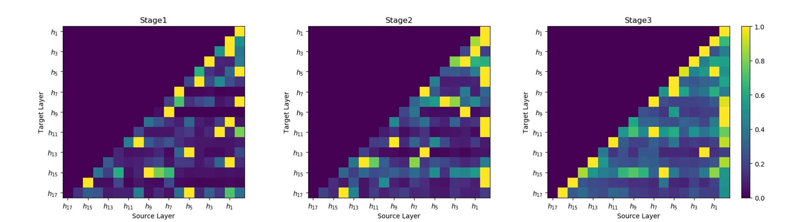
Figure 5: Visualization of feature integration for each stage by random forest. Each row presents the importance of source layers $h_{n},1\leq n<t$ contributing to the target layer $h_{t}$.

The depth of the neural network. Generally, in practice, DNNs with a larger number of parameters do not guarantee sufficient performance improvement. Deeper networks may contain extreme feature and parameter redundancy (?). Therefore, designing a new structure of deep neural networks (?; ?; ?; ?; ?; ?) is necessary. Since DIA units change the topology of DNN backbones, evaluating the effectiveness of DIANet structure is of great importance. Here we investigate how the depth of DNNs influences DIANets in two aspects: (1) the performance of DIANets compared to SENets of various depth; (2) the parameter increment of DIANets.

The results in Table 5 show that as the depth increases from 83 to 407 layers, the DIANet with a smaller number of parameters can achieve higher classification accuracy than the SENet. Moreover, the DIANet83 can achieve a similar performance as the SENet245, and DIANet164 outperforms all the SENets with at least 1.13% and at most 58.8% parameter reduction. They imply that the DIANet is of higher parameter efficiency than SENet. The results also suggest that: for DIANet, as shown in Figure 3, the DIA-LSTM unit will pass more layers recurrently with a deeper depth. The DIA-LSTM can handle the interrelationship between the information of different layers in much deeper DNN and figure out the long-distance dependency between layers.

CIFAR-100	SENet		DIANet($r=4$)
Depth	$\#$P(M)	top1-acc.	$\#$P(M)	top1-acc.
ResNet83	0.99	74.67	1.11(+0.12)	75.02
ResNet164	1.93	75.03	1.95(+0.02)	76.67
ResNet245	2.87	75.03	2.78(-0.09)	76.79
ResNet407	4.74	75.54	4.45(-0.29)	76.98

Table 5: Test accuracy (%) with ResNet of different depth on CIFAR100.

Activation function and the number of stacking LSTM cells. We choose different activation functions in the output layer of LSTM in Figure 4 (Bottom) and different numbers of stacking LSTM cells to explore the effects of these two factors. In Table 6, we find that the performance has been significantly improved after replacing tanh in the standard LSTM with sigmoid. As shown in Figure 4 (Bottom), this activation function is located in the output layer and directly changes the effect of memory unit $c_{t}$ on the output of the output gate. In fact, the sigmoid function is used in many attention-based methods like SENet as a gate mechanism. The test accuracy of different choices of LSTM activation functions in Table 6 shows that sigmoid better helps LSTM as a gate to rescale channel features. Table 12 in the SENet paper (?) shows the performance of different activation functions like: sigmoid $>$ tanh $>$ ReLU (bigger is better), which coincides to our reported results.

When we use sigmoid in the output layer of LSTM, the increasing number of stacking LSTM cells does not necessarily lead to performance improvement but may lead to performance degradation. However, when we choose tanh, the situation is different. It suggest that, through the stacking of LSTM cells, the scale of the information flow among them is changed, which may effect the performance.

$\#$P(M)	Activation	$\#$LSTM cells	top1-acc.
1.95	sigmoid	1	76.67
1.95	tanh	1	75.24
1.95	ReLU	1	74.62
3.33	sigmoid	3	75.20
3.33	tanh	3	76.47

Table 6: Test accuracy (%) with DIANet164 of different activation function at the output layer in the modified LSTM and different number of stacking LSTM cells on CIFAR100.

Analysis

In this section, we study some properties of DIANet, including feature integration and regularization effect on stabilizing training. Firstly, the layers are connected by DIA-LSTM unit in DIANet and we can use the random forest model (?) to visualize how the current layer depends on the preceding layers. Secondly, we study the stabilizing training effect of DIANet by removing all the Batch Normalization (?) or the skip connection in the residual networks.

Feature Integration

Here we try to understand the dense connection from the numerical perspective. As shown in Figure 3 and 1, the DIA-LSTM bridges the connections between layers by propagating the information forward through $h_{t}$ and $c_{t}$. Moreover, $h_{t}$ at different layers are also integrating with $h_{t^{\prime}},1\leq t^{\prime}<t$ in DIA-LSTM. Notably, $h_{t}$ is applied directly to the features in the network at each layer $t$. Therefore the relationship between $h_{t}$ at different layers somehow reflects connection degree of different layers. We explore the nonlinear relationship between the hidden state $h_{t}$ of DIA-LSTM and the preceding hidden state $h_{t-1},h_{t-2},...,h_{1}$, and visualize how the information coming from $h_{t-1},h_{t-2},...,h_{1}$ contributes to $h_{t}$. To reveal this relationship, we consider using the random forest to visualize variable importance. The random forest can return the contributions of input variables to the output separately in the form of importance measure, e.g., Gini importance (?). The computation details of Gini importance can be referred to the Appendix. Take $h_{n},1\leq n<t$ as input variables and $h_{t}$ as output variable, we can get the Gini importance of each variable $h_{n},1\leq n<t$. ResNet164 contains three stages, and each stage consists of 18 layers. We conduct three Gini importance computation to each stage separately. As shown in Figure 5, each row presents the importance of source layers $h_{n},1\leq n<t$ contributing to the target layer $h_{t}$. In each sub-graph of Figure 5, the diversity of variable importance distribution indicates that the current layer uses the information of the preceding layers. The interaction between shallow and deep layers in the same stage reveals the effect of implicitly dense connection. In particular, taking $h_{17}$ in stage 1 (the last row) as an example, $h_{16}$ or $h_{15}$ does not intuitively provide the most information for $h_{17}$, but $h_{5}$ does. We conclude that the DIA unit can adaptively integrate information between multiple layers.

stage removed	$\#$P(M)	$\#$P(M)$\downarrow$	top1-acc.	top1-acc.$\downarrow$
stage1	1.94	0.01	76.27	0.40
stage2	1.90	0.05	76.25	0.42
stage3	1.78	0.17	75.40	1.27

Table 7: The test accuracy (%) of DIANet164 with the removal of DIA-LSTM unit in different stage.

	original		SENet		DIANet$(r=16)$
	$\#$P(M)	top1-acc.	$\#$P(M)	top1-acc.	$\#$P(M)	top1-acc.
ResNet83	0.88	nan	0.98	nan	0.94	70.58
ResNet164	1.70	nan	1.91	nan	1.76	72.36
ResNet245	2.53	nan	2.83	nan	2.58	72.35
ResNet326	3.35	nan	3.75	nan	3.41	nan

Table 8: Testing accuracy (%). We train models of different depth without BN on CIFAR-100. “nan” indicates the numerical explosion.

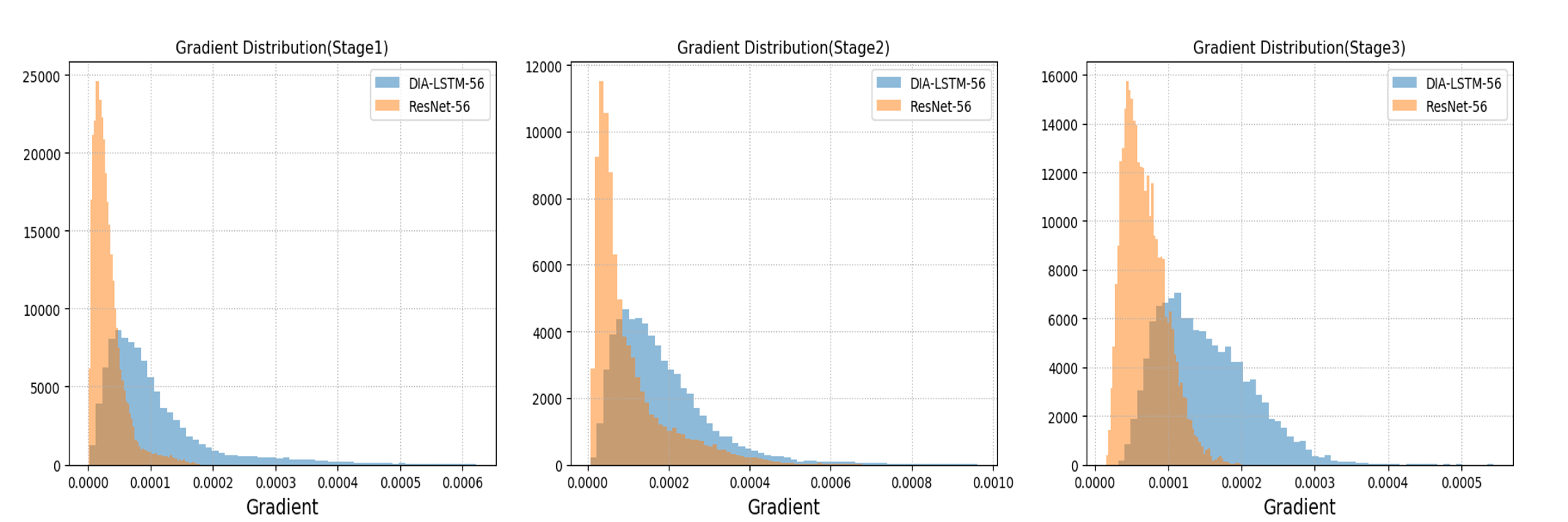
Figure 6: The distribution of gradient in each stage of ResNet56 without all the skip connections.

Moreover, in Figure 5 (stage 3), the information interaction with previous layers in stage 3 is more intense and frequent than that of the first two stages. Correspondingly, as shown in Table 7, in the experiments when we remove the DIA-LSTM unit in stage 3, the classification accuracy decreases from 76.67 to 75.40. However, when it in stage 1 or 2 is removed, the performance degradation is very similar, falling to 76.27 and 76.25 respectively. Also note that for DIANet, the number of parameter increment in stage 2 is larger than that of stage 1. It implies that the significant performance degradation after the removal of stage 3 may be not only due to the reduction of the number of parameters but due to the lack of dense feature integration.

The effect on stabilizing training

Removal of Batch Normalization. Small changes in shallower hidden layers may be amplified as the information propagates within the deep architecture and sometimes result in a numerical explosion. Batch Normalization (BN) (?) is widely used in the deep networks since it stabilizes the training by normalization the input of each layer. DIA-LSTM unit recalibrates the feature maps by channel-wise multiplication, which plays a role of scaling similar to BN. As shown in Table 8, different models trained with varying depth in CIFAR100 and BNs are removed in these networks. The experiments are conducted on a single GPU with batch size 128 and initial learning rate 0.1. Both the original ResNet, SENet face problem of numerical explosion without BN while the DIANet can be trained with depth up to 245. In Table 8, at the same depth, SENet has larger number of parameters than DIANet but still comes to numerical explosion without BN, which means that the number of parameter is not the case for stabilization of training but sharing mechanism we proposed may be the case. Besides, comparing with Table 5, the testing accuracy of DIANet without BN still can keep up to 70%. The scaling learned by DIANet integrates the information from preceding layers and enables the network to choose a better scaling for feature maps of current layer.

Removal of skip connection. The skip connection has become a necessary structure for training DNNs (?). Without skip connection, the DNN is hard to train due to the reasons like the gradient vanishing (?; ?; ?). We conduct the experiment where all the skip connections are removed in ResNet56 and count the absolute value of gradient at the output tensor of each stage. As shown in Figure 6 which presents the gradient distribution with all skip connection removal, DIANet (blue) obviously enlarges the mean and variance of the gradient distribution, which enables larger absolute value and diversity of gradient and relieves gradient degradation to some extent.

Without data augment. Explicit dense connections may help bring more efficient usage of parameters, which makes the neural network less prone to overfit (?). Although the dense connections in DIA-LSTM are implicit, the DIANet still shows the ability to reduce overfitting. To verify it, We train the models without data augment to reduce the influence of regularization from data augment. As shown in Table 9, DIANet achieves lower testing error than ResNet164 and SENet. To some extent, the implicit and dense structure of DIANet may have regularization effect.

Models	CIFAR-10	CIFAR-100
ResNet164	87.32	60.92
SENet	88.30	62.91
DIANet	89.25	66.73

Table 9: Test accuracy (%) of the models without data augment with ResNet164.

Conclusion

In this paper, we proposes a novel-and-simple framework that shares an attention module throughout different network layers to encourage the integration of layer-wise information. The parameter-sharing module is called Dense-and-Implicit Attention (DIA) unit. We propose incorporating LSTM in DIA unit (DIA-LSTM) and show the effectiveness of DIA-LSTM for image classification by conducting experiments on benchmark datasets and popular networks. We further empirically show that the DIA-LSTM has a strong regularization ability on stabilizing the training of deep networks by the experiments with the removal of skip connections or Batch Normalization (?) in the whole residual network.

Appendix A Introdcution of Implementation detail

The hyper-parameter settings of CIFAR and ImageNet are shown in Table 10 and Table 11 respectively.

	ResNet164	PreResNet164	WRN52-4	ResNext101-8x32
Batch size	128	128	128	128
Epoch	180	164	200	300
Optimizer	SGD(0.9)	SGD(0.9)	SGD(0.9)	SGD(0.9)
depth	164	164	52	101
schedule	60/120	81/122	80/120/160	150/225
wd	1.00E-04	1.00E-04	5.00E-04	5.00E-04
gamma	0.1	0.1	0.2	0.1
widen-factor	-	-	4	4
cardinality	-	-	-	8
lr	0.1	0.1	0.1	0.1
$F_{ext}(\cdot)$	GAP	BN+GAP	BN+GAP	GAP
drop	-	-	0.3	-

Table 10: Implementation detail for CIFAR10/100 image classification. Normalization and standard data augmentation (random cropping and horizontal flipping) are applied to the training data. GAP and BN denote Global Average Pooling and Batch Normalization separately.

	ResNet34	ResNet50	ResNet152	ResNext50-32x4
Batch size	256	256	256	256
Epoch	120	120	120	120
Optimizer	SGD(0.9)	SGD(0.9)	SGD(0.9)	SGD(0.9)
depth	34	50	152	50
schedule	30/60/90	30/60/90	30/60/90	30/60/90
wd	1.00E-04	1.00E-04	1.00E-04	1.00E-04
gamma	0.1	0.1	0.1	0.1
lr	0.1	0.1	0.1	0.1
$F_{ext}(\cdot)$	GAP	GAP	GAP	GAP

Table 11: Implementation detail for ImageNet 2012 image classification. Normalization and standard data augmentation (random cropping and horizontal flipping) are applied to the training data. The random cropping of size 224 by 224 is used in these experiments. GAP denote Global Average Pooling .

Batch size	train batchsize
Epoch	number of total epochs to run
Optimizer	Optimizer
depth	the depth of the network
schedule	Decrease learning rate at these epochs
wd	weight decay
gamma	learning rate is multiplied by gamma on schedule
widen-factor	Widen factor
cardinality	Model cardinality (group)
lr	initial learning rate
$F_{ext}(\cdot)$	extract features(Figure 1)
drop	Dropout ratio

Table 12: The Additional explanation

Appendix B Gini importance

We present the algorithm of computing the Gini importance used in our paper in Algorithm 1.

1:$H$: composed of $h_{1}$,$h_{2}$,…,$h_{t}$ from stage $i$; #The size of $H$ is ($b_{z}\times c_{z}\times f_{z}$) #$b_{z}$ denotes the batch size of $h_{t}$ #$c_{z}$ denotes the number of the feature maps’ channel in current stage #$f_{z}$ denotes the number of layers in current stage

2:The hotmap $G$ about the features integration for stage $i$;

3:initial $G=\emptyset$ ;

4:for $j=1$ to $f_{z}-1$ do

5:     $x\leftarrow[h_{1},h_{2},...,h_{j-1}]$;

6:     $y\leftarrow[h_{j}]$;

7:     $x$ $\leftarrow$ $x$.reshape($b_{z}$,$(f_{z}-j)\times c_{z}$);

8:     RF $\leftarrow$ RandomForestRegressor();

9:     RF.fit($x$,$y$);

10:     Gini_importances $\leftarrow$ RF.feature_importances_; #The length of Gini_importance is $(f_{z}-j)\times c_{z}$

11:     res $\leftarrow$ $\emptyset$;

12:     $s$ $\leftarrow$ 0;

13:     cnt $\leftarrow$ 0;

14:     for $k=0$ to $(f_{z}-j)$ do

15:         $s$ $\leftarrow$ $s$ + Gini_importance($k$);

16:         cnt $\leftarrow$ cnt + 1;

17:         if cnt == $c_{z}$-1 then

18:              res.add($s$);

19:              $s$ $\leftarrow$ 0;

20:              cnt $\leftarrow$ 0;

21:         end if$G$.add(res/$\max$(res));

22:     end for

23:end for

Algorithm 1 Calculate features integration by Gini importance from Random Forest

Appendix C Number of parameter of LSTM

Suppose the input $y_{t}$ is of size $N$ and the hidden state vector $h_{t-1}$ is also of size $N$.

Standard LSTM As shown in Figure (3) (Left), in the standard LSTM, there requires 4 linear transformation to control the information flow with input $y_{t}$ and $h_{t-1}$ respectively. The output size is set to be $N$. To simplify the calculation, the bias is omitted. Therefore, for the $y_{t}$, the number parameters of 4 linear transformation is equal to $4\times n\times n$. Similarly, the number parameters of 4 linear transformation with input $h_{t-1}$ is equal to $4\times n\times n$. The total of parameters equals to $8n^{2}.$

DIA-LSTM As shown in Figure (3) (Right), there is a linear transformation to reduce the dimension at the beginning. The dimension of input $y_{t}$ will reduce from $N$ to $N/r$ after the first linear transformation. The number of parameters for the linear transformation is equal to $n\times n/r$. Then the output will be passed into 4 linear transformation same as the standard LSTM. the number parameters of 4 linear transformation is equal to $4\times n/r\times n$. Therefore, for input $y_{t}$ and reduction ratio $r$, the number of parameters is equal to $5n^{2}/r$. Similarly, the number of parameters with input $h_{t-1}$ is the same as that concerning $y_{t}$. The total of parameters equals to $10n^{2}/r.$

References

- [Anderson 2005] Anderson, J. R. 2005. Cognitive psychology and its implications. Macmillan.
- [Bengio et al. 1994] Bengio, Y.; Simard, P.; Frasconi, P.; et al. 1994. Learning long-term dependencies with gradient descent is difficult. IEEE transactions on neural networks 5(2):157–166.
- [Britz et al. 2017] Britz, D.; Goldie, A.; Luong, M.-T.; and Le, Q. 2017. Massive exploration of neural machine translation architectures. arXiv preprint arXiv:1703.03906.
- [Cao et al. 2019] Cao, Y.; Xu, J.; Lin, S.; Wei, F.; and Hu, H. 2019. Gcnet: Non-local networks meet squeeze-excitation networks and beyond. arXiv preprint arXiv:1904.11492.
- [Cheng, Dong, and Lapata 2016] Cheng, J.; Dong, L.; and Lapata, M. 2016. Long short-term memory-networks for machine reading. EMNLP 2016.
- [Glorot and Bengio 2010] Glorot, X., and Bengio, Y. 2010. Understanding the difficulty of training deep feedforward neural networks. In Proceedings of the thirteenth international conference on artificial intelligence and statistics, 249–256.
- [Gregorutti, Michel, and Saint-Pierre 2017] Gregorutti, B.; Michel, B.; and Saint-Pierre, P. 2017. Correlation and variable importance in random forests. Statistics Computing 27(3):659–678.
- [He et al. 2016a] He, K.; Zhang, X.; Ren, S.; and Sun, J. 2016a. Deep residual learning for image recognition. In Computer Vision and Pattern Recognition.
- [He et al. 2016b] He, K.; Zhang, X.; Ren, S.; and Sun, J. 2016b. Identity mappings in deep residual networks. In European Conference on Computer Vision.
- [Hochreiter and Schmidhuber 1997] Hochreiter, S., and Schmidhuber, J. 1997. Long short-term memory. Neural computation 9(8):1735–1780.
- [Hu et al. 2018] Hu, J.; Shen, L.; Albanie, S.; Sun, G.; and Vedaldi, A. 2018. Gather-excite: Exploiting feature context in convolutional neural networks. In Advances in Neural Information Processing Systems, 9401–9411.
- [Hu, Shen, and Sun 2018] Hu, J.; Shen, L.; and Sun, G. 2018. Squeeze-and-excitation networks. In Proceedings of the IEEE conference on computer vision and pattern recognition, 7132–7141.
- [Huang et al. 2017] Huang, G.; Liu, Z.; Weinberger, K. Q.; and van der Maaten, L. 2017. Densely connected convolutional networks. In Computer Vision and Pattern Recognition.
- [Ioffe and Szegedy 2015] Ioffe, S., and Szegedy, C. 2015. Batch normalization: Accelerating deep network training by reducing internal covariate shift. In Proceedings of the 32Nd International Conference on International Conference on Machine Learning - Volume 37, ICML’15, 448–456. JMLR.org.
- [Krizhevsky and Hinton 2009] Krizhevsky, A., and Hinton, G. 2009. Learning multiple layers of features from tiny images. Technical report, Citeseer.
- [Li et al. 2019] Li, X.; Wang, W.; Hu, X.; and Yang, J. 2019. Selective kernel networks.
- [Li, Ouyang, and Wang 2016] Li, H.; Ouyang, W.; and Wang, X. 2016. Multi-bias non-linear activation in deep neural networks. In International conference on machine learning, 221–229.
- [Lin, Chen, and Yan 2013] Lin, M.; Chen, Q.; and Yan, S. 2013. Network in network. arXiv preprint arXiv:1312.4400.
- [Luong, Pham, and Manning 2015] Luong, M.-T.; Pham, H.; and Manning, C. D. 2015. Effective approaches to attention-based neural machine translation. arXiv preprint arXiv:1508.04025.
- [Miech, Laptev, and Sivic 2017] Miech, A.; Laptev, I.; and Sivic, J. 2017. Learnable pooling with context gating for video classification. arXiv preprint arXiv:1706.06905.
- [Mnih et al. 2014] Mnih, V.; Heess, N.; Graves, A.; et al. 2014. Recurrent models of visual attention. In Advances in neural information processing systems, 2204–2212.
- [Park et al. 2018] Park, J.; Woo, S.; Lee, J.-Y.; and Kweon, I. S. 2018. Bam: Bottleneck attention module. arXiv preprint arXiv:1807.06514.
- [Russakovsky et al. 2015] Russakovsky, O.; Deng, J.; Su, H.; Krause, J.; Satheesh, S.; Ma, S.; Huang, Z.; Karpathy, A.; Khosla, A.; Bernstein, M.; Berg, A. C.; and Fei-Fei, L. 2015. ImageNet Large Scale Visual Recognition Challenge. International Journal of Computer Vision (IJCV) 115(3):211–252.
- [Srivastava, Greff, and Schmidhuber 2015a] Srivastava, R. K.; Greff, K.; and Schmidhuber, J. 2015a. Training very deep networks. In Advances in neural information processing systems, 2377–2385.
- [Srivastava, Greff, and Schmidhuber 2015b] Srivastava, R. K.; Greff, K.; and Schmidhuber, J. 2015b. Highway networks. arXiv preprint arXiv:1505.00387.
- [Vaswani et al. 2017] Vaswani, A.; Shazeer, N.; Parmar, N.; Uszkoreit, J.; Jones, L.; Gomez, A. N.; Kaiser, Ł.; and Polosukhin, I. 2017. Attention is all you need. In Advances in neural information processing systems, 5998–6008.
- [Wang et al. 2017] Wang, F.; Jiang, M.; Qian, C.; Yang, S.; Li, C.; Zhang, H.; Wang, X.; and Tang, X. 2017. Residual attention network for image classification. In The IEEE Conference on Computer Vision and Pattern Recognition (CVPR).
- [Wang et al. 2018] Wang, X.; Girshick, R.; Gupta, A.; and He, K. 2018. Non-local neural networks. In Proceedings of the IEEE Conference on Computer Vision and Pattern Recognition, 7794–7803.
- [Wang et al. 2019] Wang, X.; Cai, Z.; Gao, D.; and Vasconcelos, N. 2019. Towards universal object detection by domain attention. CoRR abs/1904.04402.
- [Wolf and Bileschi 2006] Wolf, L., and Bileschi, S. 2006. A critical view of context. International Journal of Computer Vision 69(2):251–261.
- [Woo et al. 2018] Woo, S.; Park, J.; Lee, J.-Y.; and So Kweon, I. 2018. Cbam: Convolutional block attention module. In Proceedings of the European Conference on Computer Vision (ECCV), 3–19.
- [Xie et al. 2017] Xie, S.; Girshick, R.; Dollár, P.; Tu, Z.; and He, K. 2017. Aggregated residual transformations for deep neural networks. In Computer Vision and Pattern Recognition.
- [Xu et al. 2015] Xu, K.; Ba, J. L.; Kiros, R.; Cho, K.; Courville, A.; Salakhutdinov, R.; Zemel, R. S.; and Bengio, Y. 2015. Show, attend and tell: Neural image caption generation with visual attention. In Proceedings of the 32Nd International Conference on International Conference on Machine Learning - Volume 37, ICML’15, 2048–2057. JMLR.org.
- [Zagoruyko and Komodakis 2016] Zagoruyko, S., and Komodakis, N. 2016. Wide residual networks. In BMVC.
- [Zhao et al. 2017] Zhao, B.; Wu, X.; Feng, J.; Peng, Q.; and Yan, S. 2017. Diversified visual attention networks for fine-grained object classification. IEEE Transactions on Multimedia 19(6):1245–1256.