Abstract

The machine learning literature contains several constructions for prediction intervals that are intuitively reasonable but ultimately ad-hoc in that they do not come with provable performance guarantees. We present methods from the statistics literature that can be used efficiently with neural networks under minimal assumptions with guaranteed performance. We propose a neural network that outputs three values instead of a single point estimate and optimizes a loss function motivated by the standard quantile regression loss. We provide two prediction interval methods with finite sample coverage guarantees solely under the assumption that the observations are independent and identically distributed. The first method leverages the conformal inference framework and provides average coverage. The second method provides a new, stronger guarantee by conditioning on the observed data. Lastly, our loss function does not compromise the predictive accuracy of the network like other prediction interval methods. We demonstrate the ease of use of our procedures as well as its improvements over other methods on both simulated and real data. As most deep networks can easily be modified by our method to output predictions with valid prediction intervals, its use should become standard practice, much like reporting standard errors along with mean estimates.

1 Introduction

Deep neural networks have gained tremendous popularity in the last decade due to their superior predictive performance over other machine learning algorithms. They have become the state-of-the-art algorithm in many challenging tasks such as computer vision (Krizhevsky et al.,, 2012; Karpathy et al.,, 2014), speech recognition (Hinton et al.,, 2012), natural language processing (Collobert and Weston,, 2008), and bioinformatics (Alipanahi et al.,, 2015). Despite these successes, there is a paucity of research on the uncertainty of neural network predictions on new samples.

The development of accurate prediction intervals (PIs) for neural networks is a challenging task that is only beginning to gain research interest. Several authors have provided motivation for modified loss functions intended to encourage desirable properties (Nix and Weigend,, 1994; Heskes,, 1997; Khosravi et al.,, 2011; Lakshminarayanan et al.,, 2017; Pearce et al.,, 2018; Keren et al.,, 2018; Tagasovska and Lopez-Paz,, 2018; Kuleshov et al.,, 2018). That being said, some provide a PI without a point estimate (Pearce et al.,, 2018; Keren et al.,, 2018) or use loss functions which cannot be optimized with stochastic gradient descent (Khosravi et al.,, 2011). Others have distributional assumptions (Nix and Weigend,, 1994; Lakshminarayanan et al.,, 2017) or provide intervals in which the lower bound is not guaranteed to be smaller than the upper bound (Tagasovska and Lopez-Paz,, 2018). These methods also do not provide rigorous guarantees that are desired for a PI. Uncertainty estimation of neural networks from Bayesian perspective has been analyzed by (MacKay,, 1992; Gal and Ghahramani,, 2016).

The statistics literature is full of confidence interval constructions with provable performance guarantees; however, these methods often cannot be used efficiently with modern learning machines. We use variations of well-known statistical techniques to propose two neural-network-based PIs with valid coverage claims that outperform existing methods. The core of both procedures is a neural network that outputs three values and that optimizes a modified quantile regression loss function. The first method is based on the conformal method introduced by (Vovk et al.,, 2005). Papadopoulos and Haralambous, (2011) applied standard conformal inference to neural networks to construct prediction intervals with finite sample coverage guarantee. These intervals are not specific to neural networks and do not leverage their ability to adapt to a wider class of distributions. We propose a new conformity score that is tailored to neural networks that fully exploits their flexibility. A related conformity score was simultaneously proposed by Romano et al., (2019).

In practice, it is often desirable to have a stronger coverage guarantee than average coverage. We propose a second neural-network-based PI with an approximate conditional coverage claim, where we condition on the observed data. Both proposed procedures use a sample splitting strategy, where one part of the data is used to fit a network that outputs predictions and intervals while the other part is used to adjust these intervals to be valid PIs.

In Section 1.1, we formally set up the prediction problem and explain in detail what we mean by valid PIs. This includes standard concepts such as average coverage but also the new approximate conditional coverage claim which we term Probably-Approximately-Valid (PAV). Section 2 introduces neural-network-based PIs and the algorithms to produce valid prediction intervals. Extensive simulations and real-data examples in Section 3 highlight the improvements our methods make over competing algorithms: Other methods either fail to provide adequate coverage, compromise predictive accuracy, or fail to account for heteroskedasticity.

1.1 Prediction Intervals

We consider a non-parametric regression setting, where $X$ denotes the $\mathbb{R}^{d}$-valued covariate vector and $Y$ the $\mathbb{R}$-valued response. The data set $D=(X_{i},Y_{i})_{1\leq i\leq n}$ contains $n$ i.i.d. copies of the random variable $(X,Y)$. Throughout the paper, we will write $(X,Y)$ as new random variables that are independent of our data $D$.

In general, a prediction interval $\Gamma_{\alpha}(X)=\Gamma_{D,\alpha}(X)$ is an interval-valued function of $X$, the data $D$, and the confidence level $\alpha$, such that, loosely speaking, a new observation falls within the interval with probability at least $1-\alpha$. This loose definition can be made precise in various ways.

Definition 1.

The prediction interval $\Gamma_{\alpha}(X)$ controls average coverage if

$$\mathbb{P}(Y\in\Gamma_{\alpha}(X))\geq 1-\alpha.$$ (1)

Note that the probability in equation (1) is over all of the random variables included: the new observation ($X,Y$) and the data $D$. In Section 2.1, we propose a neural-network-based inference procedure that controls average coverage.

One may object to average coverage because one would like a coverage guarantee given a particular data set instead of averaging over all potential data sets. Our second prediction interval method takes steps toward alleviating this concern. We define a notion of prediction interval validity called Probably Approximately Valid (PAV), which is inspired by the theory of probably approximately correct (PAC) learning (Valiant,, 1984). A task is PAC-learnable if, loosely speaking, regardless of the data generating distribution, one can approximate the task arbitrarily well with high probability given sufficient data. Similarly, a PAV interval provides a conditional coverage guarantee with high probability regardless of the data generating distribution. To this end, let $p(\Gamma_{\alpha}|D)$ denote the conditional probability that $\Gamma_{\alpha}(X)$ contains $Y$ conditional on $D$, i.e.,

$$p(\Gamma_{\alpha}|D)=\mathbb{P}(Y\in\Gamma_{\alpha}(X)|D).$$

Definition 2.

The prediction interval $\Gamma_{\alpha}(X)$ is Probably Approximately Valid (PAV) if for all $\epsilon>0$, all $\delta>0$ and all $n\geq n_{0}(\epsilon,\delta)$,

$$\mathbb{P}\left(p(\Gamma_{\alpha}|D)\geq 1-\alpha-\epsilon\right)\geq 1-\delta.$$ (2)

This means, $\Gamma_{\alpha}(X)$ is PAV if the conditional probability of $\Gamma_{\alpha}(X)$ covering $Y$ given $D$ is at least $1-\alpha-\epsilon$ for all but $\delta 100$% of data sets $D$. In Section 2.2, we provide a greedy algorithm that selects a neural-network-based PI that is PAV such that $n_{0}(\epsilon,\delta)$ is of order $\scalebox{0.75}[1.0]{$-$}\log(\delta)/\epsilon^{2}$. Corollary 1 shows that PAV prediction intervals can also control average coverage with proper choice of $\alpha$, $\epsilon$, and $\delta$.

Both proposed PIs are the result of a prediction-interval-specific neural network that outputs a three-dimensional vector and optimizes a loss function used in quantile regression. The next subsection describes and motivates this loss function.

1.2 The PI-specific loss function

Let $N:\mathbb{R}^{d}\to\mathbb{R}^{3}$ be a network such that $N(x)=(l(x),m(x),u(x))$, where $l,m,u:\mathbb{R}^{d}\to\mathbb{R}$ with the restriction that $l(x)\leq m(x)\leq u(x)$ for all $x\in\mathbb{R}^{d}$. We use $m(x)$ to estimate the median of $Y$ given $X$, while $l(x)$ and $u(x)$ estimate the lower and upper bounds of our PI, respectively. The monotonicity, $l(x)\leq m(x)\leq u(x)$, is easily enforced by modifying any network that outputs a triple ($z_{1},z_{2},z_{3}$) to output ($z_{1}^{\prime},z_{2}^{\prime},z_{3}^{\prime}$) given by $z_{1}^{\prime}=z_{1}$, $z_{2}^{\prime}=z_{1}^{\prime}+\text{ReLU}(z_{2}-z_{1}^{\prime})$, and $z_{3}^{\prime}=z_{2}^{\prime}+\text{ReLU}(z_{3}-z_{2}^{\prime})$. Here, ReLU$(\cdot)$ is the rectified linear unit, $\max(0,\cdot)$.

For $\tau\in[0,1]$ and $u\in\mathbb{R}$, let $h_{\tau}(u)=(\tau-\mathds{1}_{u\leq 0})u$, be the standard loss function to estimate the $\tau$th quantile. We define the level-$\tau$ loss function evaluated on $N$ at $(x,y)$ by rCl L_τ(N(x),y) & = h_τ/2(y-l(x)) + h_1/2(y-m(x))
+   h_1-τ/2(y-u(x)). Letting $|D^{\prime}|$ denote the cardinality of a set $D^{\prime}$, the empirical risk of network $N$ on $D^{\prime}\subseteq D$ is

$$\mathcal{R}_{D^{\prime},\tau}(N)=\frac{1}{|D^{\prime}|}\sum_{(X_{i},Y_{i})\in D^{\prime}}\mathcal{L}_{\tau}(N(X_{i}),Y_{i}).$$ (3)

Definition 3.

Denote the neural network $N_{D^{\prime},\tau}(x)=(l_{D^{\prime},\tau}(x),m_{D^{\prime},\tau}(x),u_{D^{\prime},\tau}(x))$ to be one that is fit on $D^{\prime}\subseteq D$ by minimizing the empirical risk $\mathcal{R}_{D^{\prime},\tau}(N)$. In the trivial case where $\tau=0$, we set $l_{0}(x)=-\infty$ and $u_{0}(x)=\infty$ for all $x\in\mathbb{R}^{d}$.

By the strong law of large numbers, the empirical risk $\mathcal{R}_{D,\tau}(N)$ converges almost surely to $\mathbb{E}[\mathcal{L}_{\tau}(N(X),Y)]$ as $|D|\to\infty$. Let $q_{\tau}(x)=\inf\{y:\mathbb{P}(Y\leq y~{}|~{}X=x)\geq\tau\}$ be the conditional $\tau$-quantile of $Y$ given $X=x$, e.g., $q_{1/2}(x)$ is the conditional median of $Y$ given $X=x$. Following standard texts (Koenker,, 2005), the triple $(q_{\tau/2}(x),q_{1/2}(x),q_{1-\tau/2}(x))$ is the minimizer of $\mathbb{E}[\mathcal{L}_{\tau}(N(X),Y)]$. For a given confidence level $\alpha\in(0,1)$, $(q_{\alpha/2}(x),q_{1/2}(x),q_{1-\alpha/2}(x))$ has the desirable properties that

$$q_{1/2}(\cdot)~{}=~{}\underset{f:\mathbb{R}^{d}\to\mathbb{R}}{\arg\min}~{}\mathbb{E}|Y-f(X)|\\$$ (4)

and

$$1-\alpha~{}=~{}\mathbb{P}(q_{\alpha/2}(X)\leq Y\leq q_{1-\alpha/2}(X))~{}|~{}X)$$ (5)

under minimal assumptions on the joint distribution of $(X,Y)$. If the problem is constrained to linear regression or M-estimation, then the estimators resulting from empirical risk minimization are consistent (Wooldridge,, 2001); however, under our minimal assumptions, it is not known whether $N_{D,\tau}(x)$ consistently estimates $(q_{\alpha/2}(x),q_{1/2}(x),q_{1-\alpha}(x))$. As the network $N_{D,\alpha}(x)$ does not generally provide the desired properties in finite samples, Section 2 provides two modifications with finite sample coverage guarantees based on sample splitting.

1.3 Comments on the network architecture

In the definition of the network $N_{D,\tau}(x)$, we only specified the output layer of the neural network and the loss function it is minimizing. The remaining network architecture can be chosen by the users in order to achieve their predictive goals. The term architecture comprises the network design (e.g. number and depth of hidden layers or dropout layers) and training parameters (e.g. number of epochs, batch size, or regularization parameters). See Goodfellow et al., (2016) and citations therein for an overview on network architecture, regularization methods, and optimization algorithms. In fact, one can use a pre-trained neural network in combination with our proposed output layer and loss function to fit a neural network with accurate predictive performance and valid prediction intervals. See Section 3 for an application to a real image dataset.

We advocate the use of a single network that outputs both the prediction and the prediction interval to ensure that the prediction is always contained in the interval. Crossing quantiles is a well-known problem in the literature (see He, (1997)) that can be easily be circumvented in this way without any loss in predictive accuracy (see Section 3).

In fact, even our proposed loss function can be modified to the users needs. For example, the midpoint estimate is not restricted to be the median; one can also use the mean squared error instead of the absolute error in the loss function in order to estimate the conditional mean. If the underlying distribution is highly skewed, however, the conditional mean is not guaranteed to be lie between $q_{\alpha/2}(x)$ and $q_{1-\alpha/2}(x)$. We note that the mean squared error of the point estimate can be written as $h_{1/2}(y-m(x))^{2}$, so that squaring the other terms of equation (1.2) puts them on the same scale.

The supplemental materials demonstrate the validity of our methods over various architectures and loss functions. As this is guaranteed by our theorems, these examples are not included in the paper.

2 Construction of valid PIs with neural networks

Let $D_{1}$ and $D_{2}$ be an arbitrary partition of $D$ into two disjoint sets. $D_{1}$ is used to select and train the network and $D_{2}$ is used to adjust the resulting intervals to provide coverage guarantees. We emphasize that all results are still valid for any data-dependent architecture, as long as the dependency is only on $D_{1}$. As all networks in this paper are fit using $D_{1}$, we simplify our notation, setting $N_{\tau}(x)=N_{D_{1},\tau}(x)$ and analogously for $l_{\tau}(x)$, $m_{\tau}(x)$ and $u_{\tau}(x)$.

2.1 Average Coverage

To achieve average coverage, we use methods derived from conformal inference (Vovk et al.,, 2005; Lei et al.,, 2018). In general, conformal prediction intervals require a fixed prediction procedure that is refit on an augmented data set. As it would clearly be infeasible to refit a large network many times, this process can be simplified by using classical sample slitting. Lei et al., (2018) refer to such methods as split-conformal.

For a given $x\in\mathbb{R}^{d}$ and $y\in\mathbb{R}$, the interval $[l_{\tau}(x),u_{\tau}(x)]$ may not contain $y$; however, with $c$ given by

$$c=\max\left(\frac{m_{\tau}(x)-y}{m_{\tau}(x)-l_{\tau}(x)},\frac{y-m_{\tau}(x)}{u_{\tau}(x)-m_{\tau}(x)}\right),$$

$y$ is an endpoint of the interval $\Gamma_{\tau}^{c}(x)=[m_{\tau}(x)-c(m_{\tau}(x)-l_{\tau}(x)),m_{\tau}(x)+c(u_{\tau}(x)-m_{\tau}(x))]$, and hence is contained in $\Gamma_{\tau}^{c}(x)$. These facts can be used in a conformal inference procedure to calibrate the PI. In essence, a constant $\hat{c}\in(0,\infty)$ is chosen such that at least (1-$\alpha$)100% of the observations in the hold-out data, $D_{2}$, are contained in the interval $\Gamma_{\tau}^{\hat{c}}(X)$. Details are given in Algorithm 1.

Algorithm 1 Split Conformal Prediction Intervals

  Input: Holdout data $D_{2}$, network $N_{\tau}(x)$.

  Output: Scaled network $N_{\tau}^{\hat{c}}(x)$ with parameter $\hat{c}$.

  Set: $c_{i}=\max\left(\frac{m_{\tau}(X_{i})-Y_{i}}{m_{\tau}(X_{i})-l_{\tau}(X_{i})},\frac{Y_{i}-m_{\tau}(X_{i})}{u_{\tau}(X_{i})-m_{\tau}(X_{i})}\right)$ for    all $(X_{i},Y_{i})\in D_{2}$.

  Set: $\hat{c}$ = $c_{(k)}$, $k=\left\lceil(1-\alpha)(|D_{2}|+1)\right\rceil$ and $c_{(k)}$    the $k$th order statistic.

  Set: $l_{\tau}^{\hat{c}}(x)=m_{\tau}(x)-\hat{c}(m_{\tau}(x)-l_{\tau}(x))$ and    $u_{\tau}^{\hat{c}}(x)=m_{\tau}(x)+\hat{c}(u_{\tau}(x)-m_{\tau}(x))$.

  Return: $N_{\tau}^{\hat{c}}(x)=(l_{\tau}^{\hat{c}}(x),m_{\tau}(x),u_{\tau}^{\hat{c}}(x))$.

Theorem 1.

Let $N_{\tau}(x)=N_{D_{1},\tau}(x)$ be as in Definition 3 and $N_{\tau}^{\hat{c}}(x)$ be the result of Algorithm 1. Set $\Gamma_{\alpha}^{\hat{c}}(x)=[l_{\tau}^{\hat{c}}(x),u_{\tau}^{\hat{c}}(x)]$. Then $\mathbb{P}\left(Y\in\Gamma_{\alpha}^{\hat{c}}(X)\right)\geq 1-\alpha.$

Note that Theorem 1 also holds for any data-dependent $\hat{\tau}$ as long as the dependence of $\hat{\tau}$ on the data is only through $D_{1}$. As $\tau$ controls the width of the estimated interval and that is precisely what $\hat{c}$ is selected to calibrate, we suggest setting $\tau=\alpha$ in practice. In the simulations of Section 3, we typically observe $\hat{c}\geq 1$ for $N_{\alpha}(x)$, but $\hat{c}\to 1$ as $|D_{1}|$ increases, suggesting that $N_{\alpha}(x)$ has asymptotic $1-\alpha$ average coverage.

Proof of Theorem 1.

Because the network $N_{\tau}(x)$ is fit on $D_{1}$ which is independent of $D_{2}$, the statistics $c_{i}$ are i.i.d. conditional on $D_{1}$. For the new observation $(X,Y)$, set

$$c^{\prime}=\max\left(\frac{m_{\tau}(X)-Y}{m_{\tau}(X)-l_{\tau}(X)},\frac{Y-m_{\tau}(X)}{u_{\tau}(X)-m_{\tau}(X)}\right).$$

Conditional on $D_{1}$, $c^{\prime}$ is independent of $c_{i}$, has the same distribution as $c_{i}$, and the rank of $c^{\prime}$ among the $c_{i}$s is uniform over the set of integers $\{1,2,\ldots,|D_{2}|+1\}$. Therefore, $\mathbb{P}(c^{\prime}>c_{(k)}~{}|~{}D_{1})\leq\alpha$, where $k=\left\lceil(1-\alpha)(|D_{2}|+1)\right\rceil$ and $c_{(k)}$ is the $k$th order statistic of the $c_{1},\dots,c_{n}$. But this implies $\mathbb{P}(Y\in\Gamma_{\alpha}^{\hat{c}}(X)~{}|~{}D_{1})\geq 1-\alpha$. ∎

If ties among $c_{i}$s only happen on a set of measure 0, or if we use a random tie-breaking rule, the probability of coverage can be upper bounded by $1-\alpha+1/(|D_{1}|+1)$, meaning that the intervals are not unnecessarily wide (cf. Theorem 2.2 of Lei et al., (2018)). Algorithm 1 is a modified version of the Split-Conformal algorithm of Lei et al., (2018). Our statistics $c_{i}$ are tailored to our neural network which outputs an ordered triple, whereas previous algorithms use the residuals $R_{i}=|Y_{i}-m(X_{i})|$ or standardized variants.

2.2 PAV

In order to provide PAV intervals, we select $\hat{\tau}$ using $D_{2}$ so that $l_{\hat{\tau}}(x)$ and $u_{\hat{\tau}}(x)$ adaptively estimate the quantiles $q_{\alpha/2}(x)$ and $q_{1-\alpha/2}$. This adaptation is required as we are not guaranteed that $l_{\alpha}(x)$ and $u_{\alpha}(x)$ accurately estimate these quantities. Let $\hat{p}(N_{\tau},D_{2})$ be the empirical coverage probability of the neural network $N_{\tau}$ on the data set $D_{2}$, i.e.,

$$\hat{p}(N_{\tau},D_{2})=\frac{1}{|D_{2}|}\sum_{(X_{i},Y_{i})\in D_{2}}\mathds{1}_{Y_{i}\in[l_{\tau}(X_{i}),u_{\tau}(X_{i})]}.$$

We choose a parameter $\hat{\tau}$ over a grid $G_{K}$, where

$$G_{K}=\{\tau_{(1)},\dots,\tau_{(K)})\},\quad 1>\tau_{(1)}>\dots\tau_{(K)}>0,$$

such that the network $N_{\hat{\tau}}(x)$ has $1-\alpha$ coverage on $D_{2}$. Details are given in Algorithm 2.

Algorithm 2 PAV Prediction Intervals

  Input: Holdout data $D_{2}$, a grid $G_{K}$, Networks $N_{\tau}(x)$ with $\tau\in G_{K}$.

  Output: Network $N_{\hat{\tau}}(x)$.

  Set: $\hat{\tau}=0$.

  For $i=1$ to $K$:  If $\hat{p}(N_{\tau{(i)}},D_{2})\geq 1-\alpha$:   Set: $\hat{\tau}=\tau_{(i)}$.   End.

  Return: $N_{\hat{\tau}}(x)$.

Theorem 2.

Let $N_{\tau}(x)=N_{D_{1},\tau}(x)$ be as in Definition 3 and $N_{\hat{\tau}}(x)$ be the result of Algorithm 2. Set $\Gamma_{\alpha}^{\hat{\tau}}(x)=[l_{\hat{\tau}}(x),u_{\hat{\tau}}(x)]$. Set $p(\Gamma_{\alpha}^{\hat{\tau}}|D)=\mathbb{P}(Y\in\Gamma_{\alpha}^{\hat{\tau}}(X)~{}|~{}D)$ and $n_{2}=|D_{2}|$. Then,

$$\mathbb{P}\left(p(\Gamma_{\alpha}^{\hat{\tau}}|D)\leq 1-\alpha-\epsilon\right)\leq K\exp(-2\epsilon^{2}n_{2}).$$

The theorem continues to hold for any data-dependent grid, $\hat{G}_{K}$, as long as the dependence of $\hat{G}_{K}$ on the data is only through $D_{1}$. Given the tendency of flexible models such as neural networks to over-fit the data, $[l_{\alpha}(x),u_{\alpha}(x)]$ typically under-covers in finite samples. As such, we suggest setting $G_{K}\subseteq[0,\alpha]$, and in the simulations of Section 3 we typically observe $\hat{\tau}\leq\alpha$ but that $\hat{\tau}\to\alpha$ from below as $|D_{1}|$ increases. Note that by solving the equation $\delta=K\exp(\scalebox{0.75}[1.0]{$-$}2\epsilon^{2}n_{2})$, we get that for all $n_{2}\geq n(\epsilon,\delta,K)=\scalebox{0.75}[1.0]{$-$}\log(\delta/K)/(2\epsilon^{2})$,

$$\mathbb{P}\left(p(\Gamma_{\alpha}^{\hat{\tau}}|D)\geq 1-\alpha-\epsilon\right)\geq 1-\delta.$$

Proof of Theorem 2.

By definition of $N_{\hat{\tau}}(x)$, we have rCl 3lP(p(Γ_α^^τ|D) ≤1-α- ϵ)
 & ≤ P(p(Γ_α^^τ|D) ≤^p(N_^τ, D_2) - ϵ)
= E [ P(p(Γ_α^^τ|D) ≤^p(N_^τ, D_2) - ϵ  |   D_1 ) ]. We use the union bound to bound the conditional probability within the expectation from above by

For $\tau=0$, we have $[l_{\tau}(X),u_{\tau}(X)]=[-\infty,\infty]$ and the corresponding summand in the previous expression is equal to $0$. For $\tau\neq 0$, we have $p([l_{\tau}(X),u_{\tau}(X)]~{}|~{}D)=p([l_{\tau}(X),u_{\tau}(X)]~{}|~{}D_{1})$, because the event in the first conditional probability is independent of $D_{2}$. Observe that, conditional on $D_{1}$, $\hat{p}(N_{\tau},D_{2})$ is the mean of $n_{2}$ Bernoulli-trails with mean $p([l_{\tau}(X),u_{\tau}(X)]~{}|~{}D_{1})$. By Hoeffding’s inequality, the corresponding summand in the previous expression is bounded by $\exp(\scalebox{0.75}[1.0]{$-$}2\epsilon^{2}n_{2})$. ∎

Even though the PAV interval $\Gamma_{\alpha}^{\hat{\tau}}(X)$ does not generally provide average coverage, this can be achieved by defining a more conservative PAV interval.

Corollary 1.

Fix $\epsilon>0$ such that $\alpha-\epsilon>0$. Let $\Gamma_{\alpha-\epsilon}^{\hat{\tau}}(x)$ be defined as in Theorem 2 with $\alpha-\epsilon$ replacing $\alpha$. For all

$$n_{2}\geq\frac{-2\log(\epsilon/(2K(1-\alpha+\epsilon/2)))}{\epsilon^{2}}$$

we have

$$\mathbb{P}\left(Y\in\Gamma_{\alpha-\epsilon}^{\hat{\tau}}(X)\right)\geq 1-\alpha.$$

To prove the result observe that $\mathbb{P}(Y\in\Gamma_{\alpha-\epsilon}^{\hat{\tau}}(X))\geq(1-\alpha+\epsilon/2)(1-K\exp(\scalebox{0.75}[1.0]{$-$}\epsilon^{2}n_{2}/2)).$

2.3 Discussion of contributions

The split-conformal and adaptive selection approaches of the previous subsections admittedly constitute a revival of sample splitting. Practitioners have long used sample-splitting as a valid, tractable method for tuning or testing and can easily implement it. The methodology followed in this paper differs subtly but significantly from the standard use of sample splitting or conformal inference. Typically one creates either residuals or standardized residuals in order to estimate an additive adjustment factor for creating a PI of the form estimate $\pm$ error. It is clear that such intervals may not be appropriate for skewed or multimodal distributions. Instead of designing more complex standardizations for residuals, this paper leverages the power of NN in order to estimate the quantiles directly, using subsequent adjustments for finite sample guarantees.

We conjecture that the desirable properties in equations (4) and (5) are satisfied in a well-defined asymptotic setting: First, neural networks are universal approximators (cf. Cybenko, (1989); Hornik, (1991)). Second, given a sufficiently large data set, and under the assumption that we can minimize the empirical risk, a neural network is able to learn the conditional mean of $Y$ given $X$ (cf. Bauer and Kohler, (2017)). This conjecture is supported by simulation evidence presented in the supplement where we observe that $N_{D,\tau}(x)\to(q_{\alpha/2}(x),q_{1/2}(x),q_{1-\alpha/2}(x))$ as $|D|\to\infty$.

We propose PIs with average coverage control and an approximate conditional coverage control (PAV). A stronger coverage claim would be to control the conditional coverage probability, conditional on the input $X$. However, this only achievable under much more restrictive assumptions. Also, we note that our only (and crucial) assumption is i.i.d.-ness of the data. This means, our PIs are in general not valid for out-of-distribution samples.

3 Simulations

Throughout this section, we refer to $\Gamma_{\alpha}^{\hat{c}}(X)$ from Section 2.1 as conf-nn and $\Gamma_{\alpha}^{\hat{\tau}}(X)$ from Section 2.2 as pav. We compare our methods to 5 different procedures that use different types of loss functions that are designed to fit neural networks that output PIs. The first (conf-fw) is the classical, “fixed-width” conformal method that uses the absolute residuals as conformity score to create valid PIs (Papadopoulos and Haralambous,, 2011). The second method (high-q) is the so-called “high-quality” driven method of Pearce et al., (2018). This method uses a loss function that penalizes in-sample mis-coverage and interval length. The third method (neg-ll) uses the Gaussian negative-log-likelihood to estimate the mean and variance of the target (Nix and Weigend,, 1994). The fourth method is the calibrated regression model of Kuleshov et al., (2018), where the Gaussian negative-log-likelihood is used to estimate the distribution and and isotonic regression for calibration. Because of its probabilistic approach, we refer to this method as bayes. Finally, we also consider the interval $\Gamma_{\alpha}(X)$ (qreg-un), i.e., the unadjusted interval function of the network $N_{\alpha}(X)$.

In all data examples, we split the data $D$ into a training set $D_{1}$, a validation set $D_{2}$, and a test set $D_{3}$. $D_{1}$ is used to train the network, $D_{2}$ is used to calibrate the intervals for pav, conf-nn, conf-fw and bayes. Because neg-ll and high-q were very sensitive to the choice of hyperparameters in our experiments, we used $D_{1}$ to train these networks and $D_{2}$ for hyperparameter selection. All data experiments set $\alpha=.1$ and calculate results using $D_{3}$, which was unseen by the models. The $\hat{\tau}$ in $\Gamma_{\alpha}^{\hat{\tau}}(X)$ is selected on the grid $G_{10}=\{.1,.09,\ldots,.01\}$ and we set $\tau=\alpha$ when constructing $\Gamma_{\alpha}^{\hat{c}}(X)$. In all experiments, we used the Adam optimizer with learning rate 0.01 and no learning rate decay. The number of epochs was chosen by cross-validation on $D_{1}$. In each data example, the same network architecture is used for all methods and is trained in Python using the PyTorch library (Paszke et al.,, 2017). These architectures are described along with the data examples. All computations were performed on a Google-Cloud-Platform instance with a NVIDIA Tesla K80 GPU.

3.1 Artificial data

We simulate covariates $X\in[0,1]^{100}$, where each entry is drawn i.i.d. from a standard uniform distribution. The response is given by

$$Y=f(\beta^{\prime}X)+\epsilon,\quad\epsilon\sim N(0,1+(\beta^{\prime}X)^{2}),$$

where $f(x)=2\sin(\pi x)+\pi x$ and only the first 5 components of $\beta\in\{0,1\}^{100}$ are non-zero and equal to 1. This is a challenging setting because the model is sparse, non-linear in $X$, and heteroskedastic in $Y$ given $X$. We compare all the methods to an oracle that knows this data-generating process and thus the true conditional median, $q_{1/2}(X)=f(\beta^{\prime}X)$, as well as the uniformly most accurate, unbiased PI, $f(\beta^{\prime}X)\pm z_{\alpha/2}\sqrt{1+(\beta^{\prime}X)^{2}}$, where $z_{\alpha/2}$ is the $(1-\alpha/2)$-quantile of the standard normal distribution. We generate $|D_{1}\cup D_{2}|=100,000$ and used $3/4$ of the data for training and $1/4$ for validation. In the supplement, we provide results for data set sizes ranging between 5,000 and 100,000 with comparable results. We repeated the experiment 10 times. For each method, we train a neural network with one hidden layer and 200 hidden nodes using 80-100 passes through the data. An independent data set of size 20,000 is used for testing.

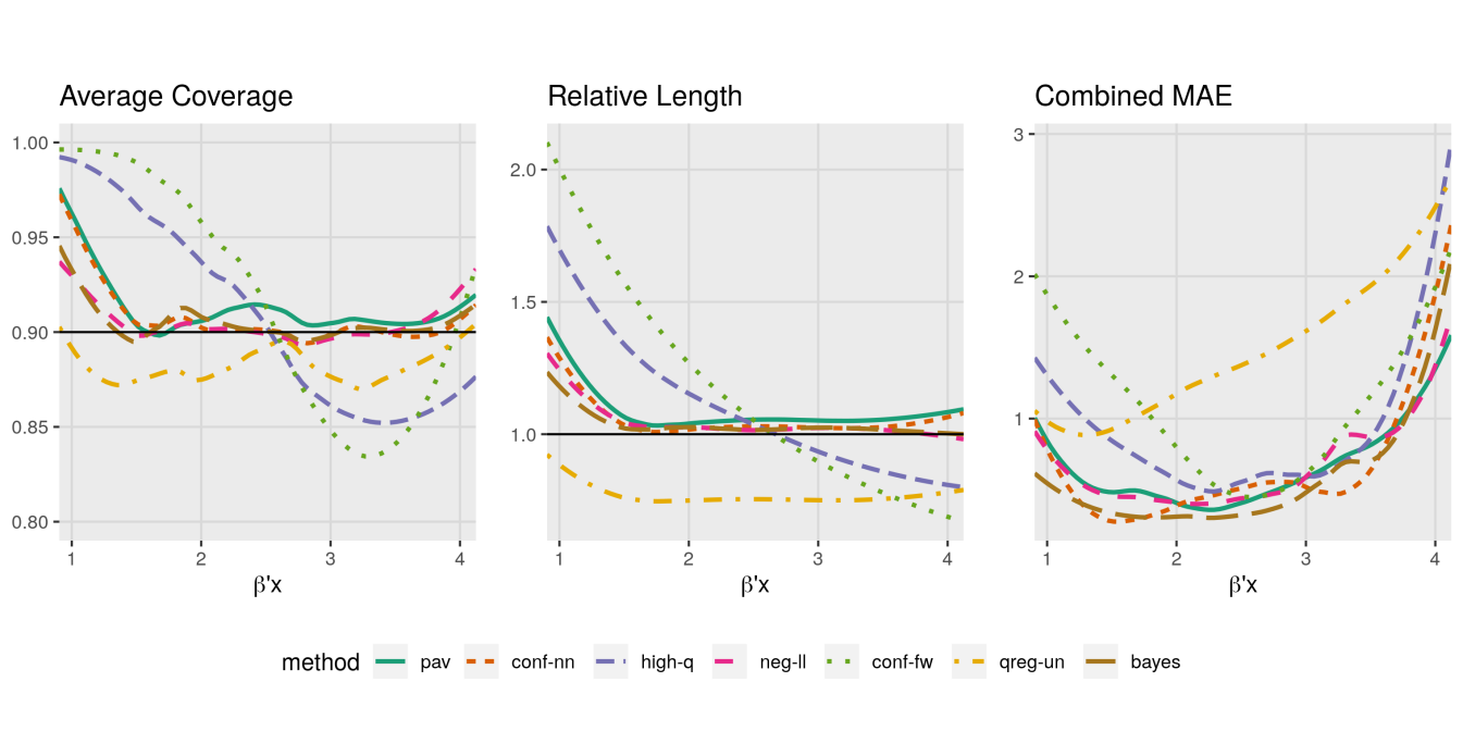
Figure 1: Results on Simulated Data. Each measure is plotted as a function of the true linear component, $\beta^{\prime}X$. The combined MAE is the mean absolute error for estimating the oracle: ($q_{1/2}(X)$, $q_{\alpha/2}(X)$, $q_{1-\alpha/2}(X)$).

Simulation results are summarized in Figure 1, which shows the empirical coverage, the interval length relative to the oracle, and the mean absolute error (MAE) from estimating ($q_{1/2}(X)$, $q_{\alpha/2}(X)$, $q_{1-\alpha/2}(X)$). Each measure is plotted as a function of $\beta^{\prime}X$ in order to observe how various methods adapt to heteroskedasticity. Both conf-nn and pav provide coverage close to the nominal level throughout the majority of the domain of $\beta^{\prime}X$. Only for small $\beta^{\prime}X$, the two methods are too wide. This can be explained by the fact that in this area only a few observations are available (see the data generation process) to estimate the conditional quantiles. This demonstrates that both procedures are accurately estimating the true underlying distribution on a wide range of the input space. bayes and neg-ll perform equally well, which is not surprising because both procedures minimize the Gaussian negative-log-likelihood. In terms of length and estimation error, conf-nn, pav, bayes and neg-ll all provide quality estimates for a wide range of $\beta^{\prime}X$.

conf-fw and high-q on the other hand over-cover in the left tail and undercover in the right tail as they do not capture the heteroscedasticity of the true distribution. This is observed in their lengths relative to the oracle. We see that qreg-un undercovers through the entire input space, which confirms the need for calibration.

3.2 Real Data

In each of the real data examples, the ratio of observations in $D_{1}$, $D_{2}$ and $D_{3}$ was equal to 3:1:1. Each experiment was repeated 20 times, i.e., the data set is randomly partitioned into three parts, then the model is trained on $D_{1}$, tuned on $D_{2}$, and evaluated on $D_{3}$. This process constitutes one repetition. We discuss the results from four real datasets here, about which further information is given in the supplement. When applicable, covariates were standardized to have mean 0 and variance 1.

We consider two datasets from the data science platform Kaggle and two from the UCI machine learning repository (Dua and Graff,, 2017). The first is a bike share dataset from UCI that contains the hourly count of bike rentals in the Capital bikeshare system along with weather information between 2011 and 2012 (Fanaee-T and Gama,, 2013). The task is to predict the number of bike rentals based on weather information. The other UCI dataset provides hourly traffic volume, westbound on I-94, in Minneapolis-St Paul, Minnesota between 2012 and 2018. The dataset also includes weather and holiday information. For both datasets, we trained a network with one hidden layer and 100 hidden nodes.

From Kaggle, we consider an image data set and a standard regression task. The image dataset contains 12,611 observations, each consisting of an x-ray of a patient’s hand. The task is to predict the patient’s age using the x-ray. We use an intermediate layer of the pre-trained Inception V3 network as the feature extractor (Szegedy et al.,, 2016). We trained a neural network on the extracted features with one hidden layer and $300$ hidden nodes. We used data augmentation (random rotation and horizontal flips of the images) on $D_{1}$ to reduce over-fitting. The regression dataset consists of 21,613 sale prices for homes in King County, Washington, between May 2014 and May 2015. There are 19 covariates describing the features of the house which are used to predict log sale price. For each method we trained a neural network with one hidden layer, with 100 hidden nodes, and between 80 and 200 passes through the data.

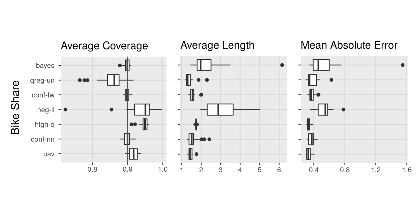
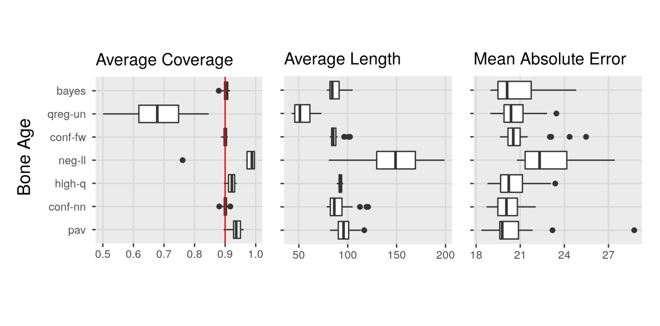
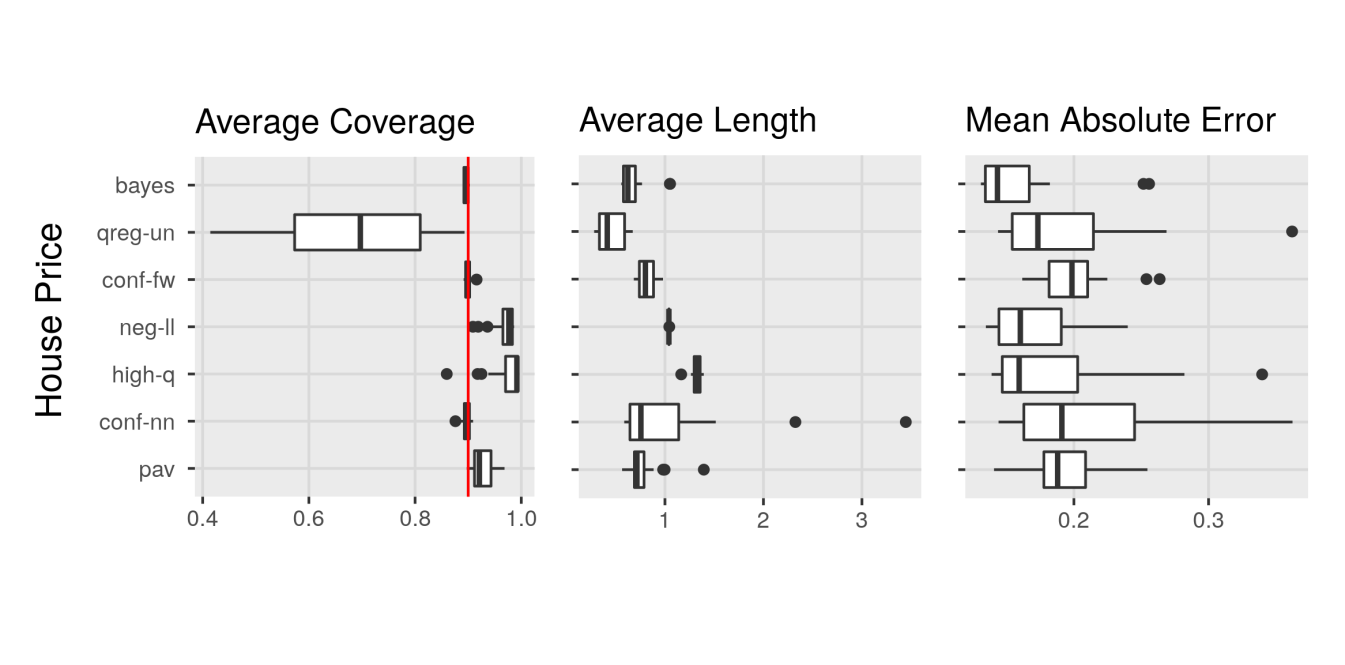
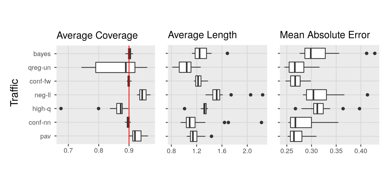
Figure 2: Summary of results on real data. Each row corresponds to a different data set and are organized alphabetically. The red line in the left-most plots denote the nominal confidence level.

Figure 2 summarizes the results on these data. It shows the empirical coverage, the average length, and the mean absolute error (MAE) of each method for predicting the target. Starting with average coverage, we see that conf-nn and pav provide average coverage at nearly exact nominal level for all repetitions and all datasets as guaranteed by our theorems. We can see that pav is more conservative, due to its stronger guarantee, though potentially also due to the coarse selection grid for $\tau$. The unadjusted method, qreg-un, does not provide coverage, which confirms our presumption that the neural network $N_{\alpha}(X)$ fails to accurately estimate the conditional quantiles in finite samples. This also strongly affirms the necessity to adjust neural network based intervals. bayes also provides precise coverage and the remaining methods primarily over-cover, partitulcarly neg-ll. We see that high-q does not provide consistent coverage on the Traffic data and found it to be highly-sensitive to hyperparameters.

Among the valid methods, conf-nn and pav are always among the shortest intervals. bayes performs significantly worse on the Bike Share and traffic datasets, with many repetitions having double or triple the length and error of conf-nn and pav. While conf-fw provides surprisingly short intervals on average, we note that in the presence of heteroscedasticity it can occur that inferior fixed-width intervals are narrower, on average, than the optimal intervals. high-q is slightly wider and neg-ll is considerably wider on average, also showing they they can be too conservative.

In terms of the estimation error conf-nn, pav and conf-fw have similar performance on all datasets. We emphasize this as conf-fw fits a neural network that minimizes mean absolute error directly, while conf-nn and pav both use the loss function given (1.2). This demonstrates that our proposed loss function does not comprise the predictive accuracy of the fitted networks.

4 Conclusion

In this paper we demonstrated how to use standard statistical techniques such as sample splitting and quantile regression to fit a neural network that outputs accurate predictions and valid prediction intervals. We proposed two procedures with provable coverage guarantees that improve current state-of-the-art methods in terms of interval length and predictive accuracy. The ease and transparency of the two procedures advocate their application to many deep neural networks in order to express the uncertainty of their predictions. As data sets grow in size, the cost of using a validation set decreases, making the observation of Barnard, (1974) even more accurate today:

The simple idea of splitting a sample into two and then developing the hypothesis on the basis of one part and testing it on the remainder may perhaps be said to be one of the most seriously neglected ideas in statistics, if we measure the degree of neglect by the ratio of the number of cases where a method could give help to the number of cases where it is actually used.

References

- Alipanahi et al., (2015) Alipanahi, B., Delong, A., Weirauch, M. T., and Frey, B. J. (2015). Predicting the sequence specificities of dna-and rna-binding proteins by deep learning. Nature biotechnology, 33(8):831.
- Barnard, (1974) Barnard, G. A. (1974). Discussion of “cross-validatory choice and assessment of statistical predictions,” by m. stone. Journal of the Royal Statistical Society: Series B (Methodological), 36(2):133–135.
- Bauer and Kohler, (2017) Bauer, B. and Kohler, M. (2017). On deep learning as a remedy for the curse of dimensionality in nonparametric regression. Submitted for publication.
- Collobert and Weston, (2008) Collobert, R. and Weston, J. (2008). A unified architecture for natural language processing: Deep neural networks with multitask learning. In Proceedings of the 25th international conference on Machine learning, pages 160–167. ACM.
- Cybenko, (1989) Cybenko, G. (1989). Approximation by superpositions of a sigmoidal function. Mathematics of control, signals and systems, 2:303–314.
- Dua and Graff, (2017) Dua, D. and Graff, C. (2017). UCI machine learning repository.
- Fanaee-T and Gama, (2013) Fanaee-T, H. and Gama, J. (2013). Event labeling combining ensemble detectors and background knowledge. Progress in Artificial Intelligence, pages 1–15.
- Gal and Ghahramani, (2016) Gal, Y. and Ghahramani, Z. (2016). Dropout as a bayesian approximation: Representing model uncertainty in deep learning. In international conference on machine learning, pages 1050–1059.
- Goodfellow et al., (2016) Goodfellow, I., Bengio, Y., and Courville, A. (2016). Deep Learning. MIT Press.
- He, (1997) He, X. (1997). Quantile curves without crossing. The American Statistician, 51:186–192.
- Heskes, (1997) Heskes, T. (1997). Practical confidence and prediction intervals. In Advances in neural information processing systems, pages 176–182.
- Hinton et al., (2012) Hinton, G., Deng, L., Yu, D., Dahl, G., Mohamed, A.-r., Jaitly, N., Senior, A., Vanhoucke, V., Nguyen, P., Kingsbury, B., et al. (2012). Deep neural networks for acoustic modeling in speech recognition. IEEE Signal processing magazine, 29.
- Hornik, (1991) Hornik, K. (1991). Approximation capabilities of multilayer feedforward networks. Neural networks, 4:251–257.
- Karpathy et al., (2014) Karpathy, A., Toderici, G., Shetty, S., Leung, T., Sukthankar, R., and Fei-Fei, L. (2014). Large-scale video classification with convolutional neural networks. In Proceedings of the IEEE conference on Computer Vision and Pattern Recognition, pages 1725–1732.
- Keren et al., (2018) Keren, G., Cummins, N., and Schuller, B. (2018). Calibrated prediction intervals for neural network regressors. IEEE Access, 6:54033–54041.
- Khosravi et al., (2011) Khosravi, A., Nahavandi, S., Creighton, D., and Atiya, A. F. (2011). Lower upper bound estimation method for construction of neural network-based prediction intervals. IEEE transactions on neural networks, 22:337–346.
- Koenker, (2005) Koenker, R. (2005). Quantile Regression. Econometric Society Monographs. Cambridge University Press.
- Krizhevsky et al., (2012) Krizhevsky, A., Sutskever, I., and Hinton, G. E. (2012). Imagenet classification with deep convolutional neural networks. In Advances in neural information processing systems, pages 1097–1105.
- Kuleshov et al., (2018) Kuleshov, V., Fenner, N., and Ermon, S. (2018). Accurate uncertainties for deep learning using calibrated regression. arXiv preprint arXiv:1807.00263.
- Lakshminarayanan et al., (2017) Lakshminarayanan, B., Pritzel, A., and Blundell, C. (2017). Simple and scalable predictive uncertainty estimation using deep ensembles. In Advances in Neural Information Processing Systems, pages 6402–6413.
- Lei et al., (2018) Lei, J., G’Sell, M., Rinaldo, A., Tibshirani, R. J., and Wasserman, L. (2018). Distribution-free predictive inference for regression. Journal of the American Statistical Association, 113(523):1094–1111.
- MacKay, (1992) MacKay, D. J. (1992). A practical bayesian framework for backpropagation networks. Neural computation, 4(3):448–472.
- Nix and Weigend, (1994) Nix, D. A. and Weigend, A. S. (1994). Estimating the mean and variance of the target probability distribution. In Proceedings of 1994 IEEE International Conference on Neural Networks (ICNN’94), volume 1, pages 55–60. IEEE.
- Papadopoulos and Haralambous, (2011) Papadopoulos, H. and Haralambous, H. (2011). Reliable prediction intervals with regression neural networks. Neural Networks, 24(8):842–851.
- Paszke et al., (2017) Paszke, A., Gross, S., Chintala, S., Chanan, G., Yang, E., DeVito, Z., Lin, Z., Desmaison, A., Antiga, L., and Lerer, A. (2017). Automatic differentiation in pytorch.
- Pearce et al., (2018) Pearce, T., Brintrup, A., Zaki, M., and Neely, A. (2018). High-quality prediction intervals for deep learning: A distribution-free, ensembled approach. In ICML.
- Romano et al., (2019) Romano, Y., Patterson, E., and Candès, E. J. (2019). Conformalized quantile regression. arXiv preprint arXiv:1905.03222.
- Szegedy et al., (2016) Szegedy, C., Vanhoucke, V., Ioffe, S., Shlens, J., and Wojna, Z. (2016). Rethinking the inception architecture for computer vision. In Proceedings of the IEEE conference on computer vision and pattern recognition, pages 2818–2826.
- Tagasovska and Lopez-Paz, (2018) Tagasovska, N. and Lopez-Paz, D. (2018). Frequentist uncertainty estimates for deep learning. CoRR, abs/1811.00908.
- Valiant, (1984) Valiant, L. G. (1984). A theory of the learnable. In Proceedings of the sixteenth annual ACM symposium on Theory of computing, pages 436–445. ACM.
- Vovk et al., (2005) Vovk, V., Gammerman, A., and Shafer, G. (2005). Algorithmic Learning in a Random World. Springer-Verlag, Berlin, Heidelberg.
- Wooldridge, (2001) Wooldridge, J. M. (2001). Econometric Analysis of Cross Section and Panel Data, volume 1 of MIT Press Books. The MIT Press.