Stochastic Shared Embeddings: Data-driven Regularization of Embedding Layers

Abstract

In deep neural nets, lower level embedding layers account for a large portion of the total number of parameters. Tikhonov regularization, graph-based regularization, and hard parameter sharing are approaches that introduce explicit biases into training in a hope to reduce statistical complexity. Alternatively, we propose stochastic shared embeddings (SSE), a data-driven approach to regularizing embedding layers, which stochastically transitions between embeddings during stochastic gradient descent (SGD). Because SSE integrates seamlessly with existing SGD algorithms, it can be used with only minor modifications when training large scale neural networks. We develop two versions of SSE: SSE-Graph using knowledge graphs of embeddings; SSE-SE using no prior information. We provide theoretical guarantees for our method and show its empirical effectiveness on 6 distinct tasks, from simple neural networks with one hidden layer in recommender systems, to the transformer and BERT in natural languages. We find that when used along with widely-used regularization methods such as weight decay and dropout, our proposed SSE can further reduce overfitting, which often leads to more favorable generalization results.

1 Introduction

Recently, embedding representations have been widely used in almost all AI-related fields, from feature maps [13] in computer vision, to word embeddings [15, 20] in natural language processing, to user/item embeddings [17, 10] in recommender systems. Usually, the embeddings are high-dimensional vectors. Take language models for example, in GPT [22] and Bert-Base model [3], 768-dimensional vectors are used to represent words. Bert-Large model utilizes 1024-dimensional vectors and GPT-2 [23] may have used even higher dimensions in their unreleased large models. In recommender systems, things are slightly different: the dimension of user/item embeddings are usually set to be reasonably small, 50 or 100, but the number of users and items is on a much bigger scale. Contrast this with the fact that the size of word vocabulary that normally ranges from 50,000 to 150,000, the number of users and items can be millions or even billions in large-scale real-world commercial recommender systems [1].

Given the massive number of parameters in modern neural networks with embedding layers, mitigating over-parameterization can play an important role in preventing over-fitting in deep learning. We propose a regularization method, Stochastic Shared Embeddings (SSE), that uses prior information about similarities between embeddings, such as semantically and grammatically related words in natural languages or real-world users who share social relationships. Critically, SSE progresses by stochastically transitioning between embeddings as opposed to a more brute-force regularization such as graph-based Laplacian regularization and ridge regularization. Thus, SSE integrates seamlessly with existing stochastic optimization methods and the resulting regularization is data-driven.

We will begin the paper with the mathematical formulation of the problem, propose SSE, and provide the motivations behind SSE. We provide a theoretical analysis of SSE that can be compared with excess risk bounds based on empirical Rademacher complexity. We then conducted experiments for a total of 6 tasks from simple neural networks with one hidden layer in recommender systems, to the transformer and BERT in natural languages and find that when used along with widely-used regularization methods such as weight decay and dropout, our proposed methods can further reduce over-fitting, which often leads to more favorable generalization results.

2 Related Work

Regularization techniques are used to control model complexity and avoid over-fitting. $\ell_{2}$ regularization [8] is the most widely used approach and has been used in many matrix factorization models in recommender systems; $\ell_{1}$ regularization [29] is used when a sparse model is preferred. For deep neural networks, it has been shown that $\ell_{p}$ regularizations are often too weak, while dropout [7, 27] is more effective in practice. There are many other regularization techniques, including parameter sharing [5], max-norm regularization [26], gradient clipping [19], etc.

Our proposed SSE-graph is very different from graph Laplacian regularization [2], in which the distances of any two embeddings connected over the graph are directly penalized. Hard parameter sharing uses one embedding to replace all distinct embeddings in the same group, which inevitably introduces a significant bias. Soft parameter sharing [18] is similar to the graph Laplacian, penalizing the $l_{2}$ distances between any two embeddings. These methods have no dependence on the loss, while the proposed SSE-graph method is data-driven in that the loss influences the effect of regularization. Unlike graph Laplacian regularization, hard and soft parameter sharing, our method is stochastic by nature. This allows our model to enjoy similar advantages as dropout [27].

Interestingly, in the original BERT model’s pre-training stage [3], a variant of SSE-SE is already implicitly used for token embeddings but for a different reason. In [3], the authors masked 15% of words and 10% of the time replaced the [mask] token with a random token. In the next section, we discuss how SSE-SE differs from this heuristic. Another closely related technique to ours is the label smoothing [28], which is widely used in the computer vision community. We find that in the classification setting if we apply SSE-SE to one-hot encodings associated with output $y_{i}$ only, our SSE-SE is closely related to the label smoothing, which can be treated as a special case of our proposed method.

Algorithm 1 SSE-Graph for Neural Networks with Embeddings

1:  Input: input $x_{i}$, label $y_{i}$, backpropagate $T$ steps, mini-batch size $m$, knowledge graphs on embeddings $\{E_{1},\dots,E_{M}\}$

2:  Define $p_{l}(.,.|\Phi)$ based on knowledge graphs on embeddings, $l=1,\ldots,M$

3:  for $t=1$ to $T$ do

4:     Sample one mini-batch $\{x_{1},\dots,x_{m}\}$

5:     for $i=1$ to $m$ do

6:        Identify the set of embeddings $\mathcal{S}_{i}=\{E_{1}[j^{i}_{1}],\dots,E_{M}[j^{i}_{M}]\}$ for input $x_{i}$ and label $y_{i}$

7:        for each embedding $E_{l}[j^{i}_{l}]\in\mathcal{S}_{i}$ do

8:           Replace $E_{l}[j^{i}_{l}]$ with $E_{l}[k_{l}]$, where $k_{l}\sim p_{l}(j^{i}_{l},.|\Phi)$

9:        end for

10:     end for

11:     Forward and backward pass with the new embeddings

12:  end for

13:  Return embeddings $\{E_{1},\dots,E_{M}\}$, and neural network parameters $\Theta$

3 Stochastic Shared Embeddings

Throughout this paper, the network input $x_{i}$ and label $y_{i}$ will be encoded into indices $j_{1}^{i},\ldots,j_{M}^{i}$ which are elements of $\mathcal{I}_{1}\times\ldots\mathcal{I}_{M}$, the index sets of embedding tables. A typical choice is that the indices are the encoding of a dictionary for words in natural language applications, or user and item tables in recommendation systems. Each index, $j_{l}$, within the $l$th table, is associated with an embedding $E_{l}[j_{l}]$ which is a trainable vector in $\mathbb{R}^{d_{l}}$. The embeddings associated with label $y_{i}$ are usually non-trainable one-hot vectors corresponding to label look-up tables while embeddings associated with input $x_{i}$ are trainable embedding vectors for embedding look-up tables. In natural language applications, we appropriately modify this framework to accommodate sequences such as sentences.

The loss function can be written as the functions of embeddings:

$$R_{n}(\Theta)=\sum_{i}\ell(x_{i},y_{i}|\Theta)=\sum_{i}\ell(E_{1}[j^{i}_{1}],\dots,E_{M}[j_{M}^{i}]|\Theta),$$ (1)

where $y_{i}$ is the label and $\Theta$ encompasses all trainable parameters including the embeddings, $\{E_{l}[j_{l}]:j_{l}\in\mathcal{I}_{l}\}$. The loss function $\ell$ is a mapping from embedding spaces to the reals. For text input, each $E_{l}[j^{i}_{l}]$ is a word embedding vector in the input sentence or document. For recommender systems, usually there are two embedding look-up tables: one for users and one for items [6]. So the objective function, such as mean squared loss or some ranking losses, will comprise both user and item embeddings for each input. We can more succinctly write the matrix of all embeddings for the $i$th sample as $\mathbf{E}[\mathbf{j}^{i}]=(E_{1}[j_{1}^{i}],\ldots,E_{M}[j_{M}^{i}])$ where $\mathbf{j}^{i}=(j^{i}_{1},\ldots,j^{i}_{M})\in\mathcal{I}$. By an abuse of notation we write the loss as a function of the embedding matrix, $\ell(\mathbf{E}[\mathbf{j}^{i}]|\Theta)$.

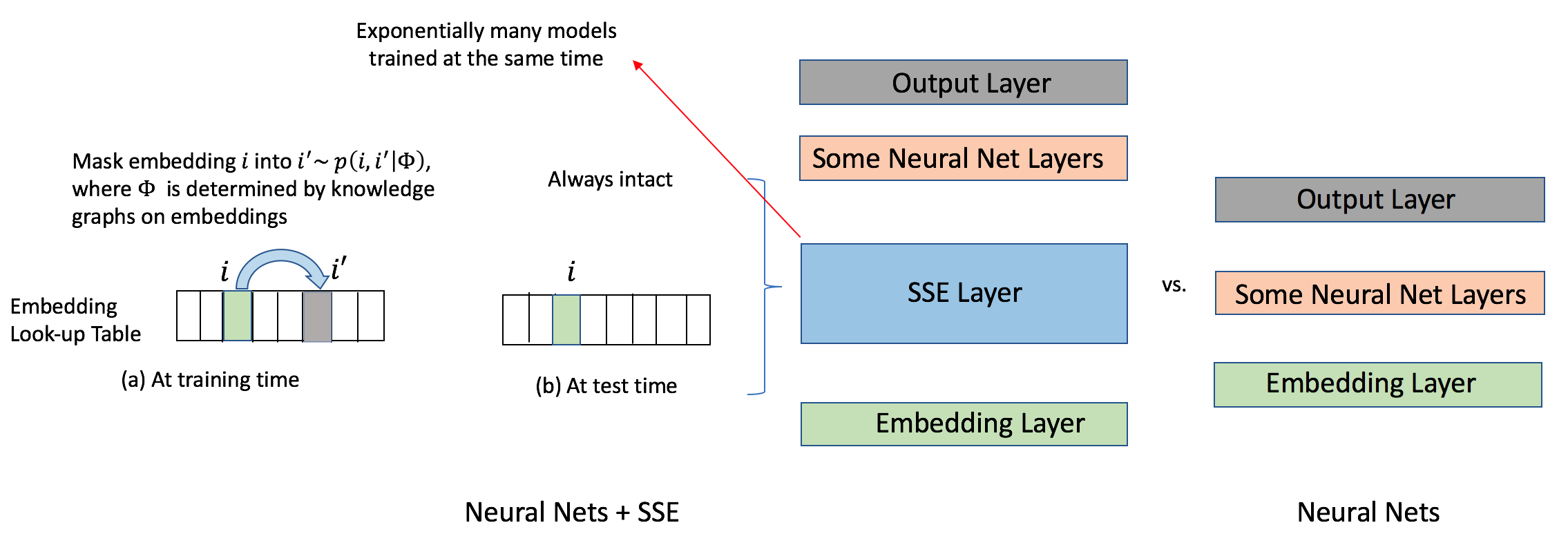
Figure 1: SSE-Graph described in Algorithm 1 and Figure 2 can be viewed as adding exponentially many distinct reordering layers above the embedding layer. A modified backpropagation procedure in Algorithm 1 is used to train exponentially many such neural networks at the same time.

Suppose that we have access to knowledge graphs [16, 14] over embeddings, and we have a prior belief that two embeddings will share information and replacing one with the other should not incur a significant change in the loss distribution. For example, if two movies are both comedies and they are starred by the same actors, it is very likely that for the same user, replacing one comedy movie with the other comedy movie will result in little change in the loss distribution. In stochastic optimization, we can replace the loss gradient for one movie’s embedding with the other similar movie’s embedding, and this will not significantly bias the gradient if the prior belief is accurate. On the other hand, if this exchange is stochastic, then it will act to smooth the gradient steps in the long run, thus regularizing the gradient updates.

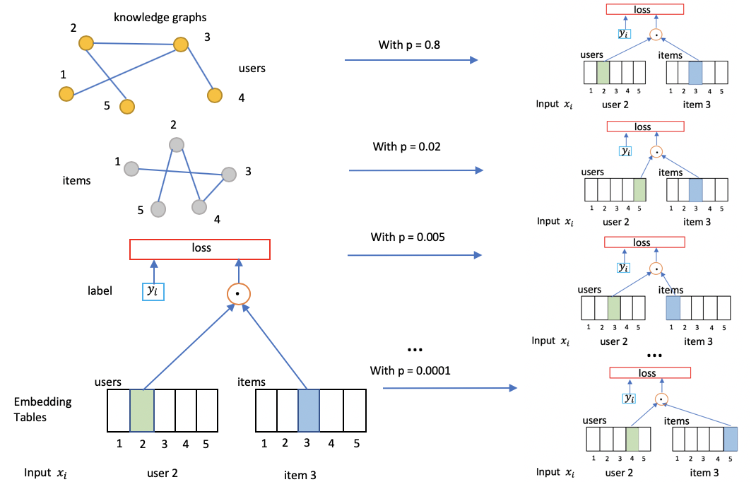
Figure 2: Illustration of how SSE-Graph algorithm in Figure 1 works for a simple neural network.

3.1 General SSE with Knowledge Graphs: SSE-Graph

Instead of optimizing objective function $R_{n}(\Theta)$ in (1), SSE-Graph described in Algorithm 1, Figure 1, and Figure 2 is approximately optimizing the objective function below:

$$S_{n}(\Theta)=\sum_{i}\sum_{\mathbf{k}\in\mathcal{I}}p(\mathbf{j}^{i},\mathbf{k}|\Phi)\ell(\mathbf{E}[\mathbf{k}]|\Theta),$$ (2)

where $p(\mathbf{j},\mathbf{k}|\Phi)$ is the transition probability (with parameters $\Phi$) of exchanging the encoding vector $\mathbf{j}\in\mathcal{I}$ with a new encoding vector $\mathbf{k}\in\mathcal{I}$ in the Cartesian product index set of all embedding tables. When there is a single embedding table ($M=1$) then there are no hard restrictions on the transition probabilities, $p(.,.)$, but when there are multiple tables ($M>1$) then we will enforce that $p(.,.)$ takes a tensor product form (see (4)). When we are assuming that there is only a single embedding table ($M=1$) we will not bold $j,E[j]$ and suppress their indices.

In the single embedding table case, $M=1$, there are many ways to define transition probability from $j$ to $k$. One simple and effective way is to use a random walk (with random restart and self-loops) on a knowledge graph $\mathcal{G}$, i.e. when embedding $j$ is connected with $k$ but not with $l$, we can set the ratio of $p(j,k|\Phi)$ and $p(j,l|\Phi)$ to be a constant greater than $1$. In more formal notation, we have

$$j\sim k,j\not\sim l\longrightarrow p(j,k|\Phi)/p(j,l|\Phi)=\rho,$$ (3)

where $\rho>1$ and is a tuning parameter. It is motivated by the fact that embeddings connected with each other in knowledge graphs should bear more resemblance and thus be more likely replaced by each other. Also, we let $p(j,j|\Phi)=1-p_{0},$ where $p_{0}$ is called the SSE probability and embedding retainment probability is $1-p_{0}$. We treat both $p_{0}$ and $\rho$ as tuning hyper-parameters in experiments. With (3) and $\sum_{k}p(j,k|\Phi)=1$, we can derive transition probabilities between any two embeddings to fill out the transition probability table.

When there are multiple embedding tables, $M>1$, then we will force that the transition from $\mathbf{j}$ to $\mathbf{k}$ can be thought of as independent transitions from $j_{l}$ to $k_{l}$ within embedding table $l$ (and index set $\mathcal{I}_{l}$). Each table may have its own knowledge graph, resulting in its own transition probabilities $p_{l}(.,.)$. The more general form of the SSE-graph objective is given below:

$$S_{n}(\Theta)=\sum_{i}\sum_{k_{1},\dots,k_{M}}p_{1}(j^{i}_{1},k_{1}|\Phi)\cdots p_{M}(j^{i}_{M},k_{M}|\Phi)\ell(E_{1}[k_{1}],\dots,E_{M}[k_{M}]|\Theta),$$ (4)

Intuitively, this SSE objective could reduce the variance of the estimator.

Optimizing (4) with SGD or its variants (Adagrad [4], Adam [12]) is simple. We just need to randomly switch each original embedding tensor $\mathbf{E}[\mathbf{j}^{i}]$ with another embedding tensor $\mathbf{E}[\mathbf{k}]$ randomly sampled according to the transition probability (see Algorithm 1). This is equivalent to have a randomized embedding look-up layer as shown in Figure 1.

We can also accommodate sequences of embeddings, which commonly occur in natural language application, by considering $(j^{i}_{l,1},k_{l,1}),\dots,(j^{i}_{l,n^{i}_{l}},k_{l,n^{i}_{l}})$ instead of $(j^{i}_{l},k_{l})$ for $l$-th embedding table in (4), where $1\leq l\leq M$ and $n^{i}_{l}$ is the number of embeddings in table $l$ that are associated with $(x_{i},y_{i})$. When there is more than one embedding look-up table, we sometimes prefer to use different $p_{0}$ and $\rho$ for different look-up tables in (3) and the SSE probability constraint. For example, in recommender systems, we would use $p_{u},\rho_{u}$ for user embedding table and $p_{i},\rho_{i}$ for item embedding table.

We find that SSE with knowledge graphs, i.e., SSE-Graph, can force similar embeddings to cluster when compared to the original neural network without SSE-Graph. In Figure 3, one can easily see that more embeddings tend to cluster into 2 singularities after applying SSE-Graph when embeddings are projected into 3D spaces using PCA. Interestingly, a similar phenomenon occurs when assuming the knowledge graph is a complete graph, which we would introduce as SSE-SE below.

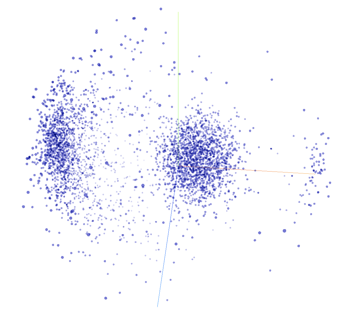
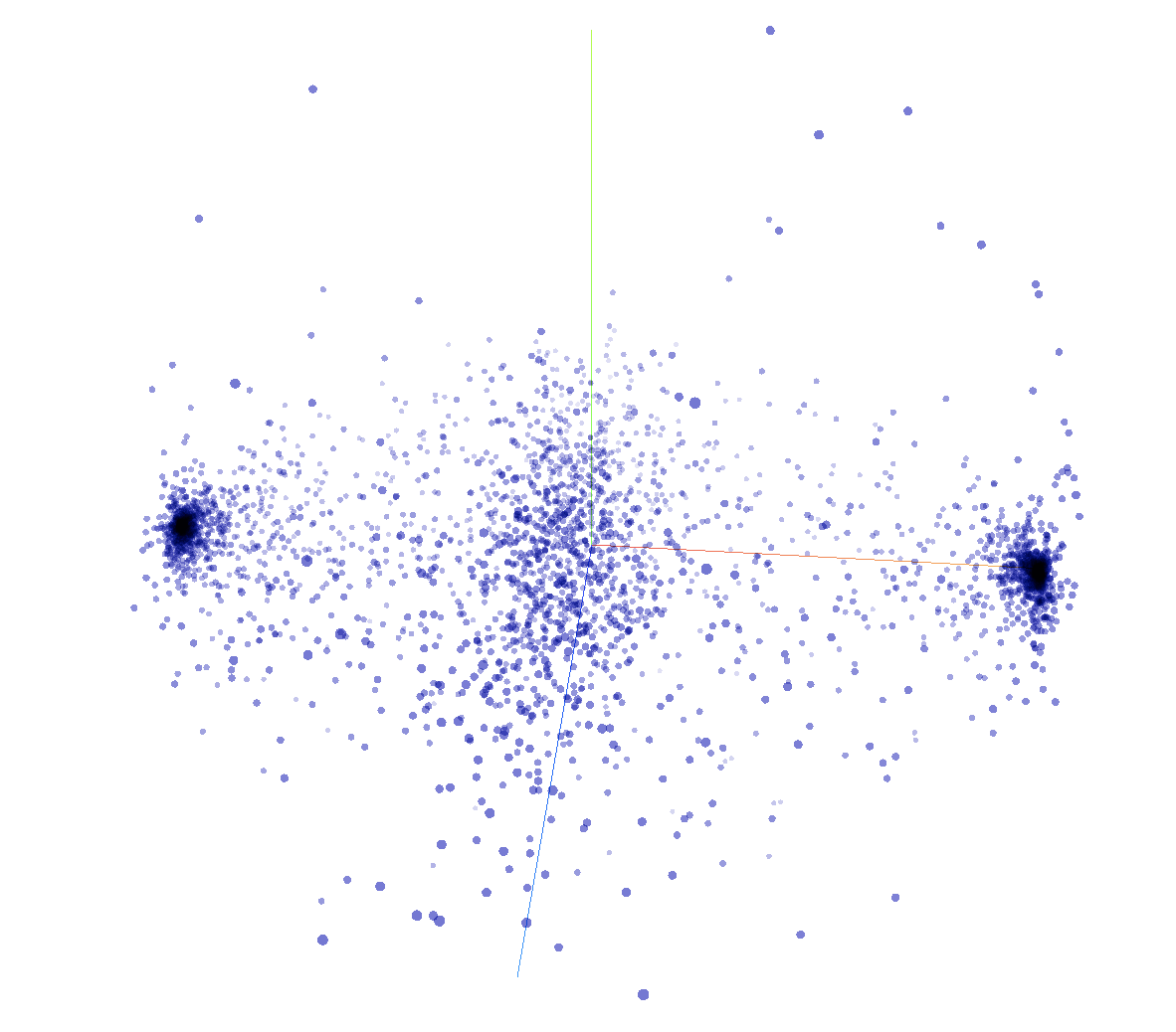
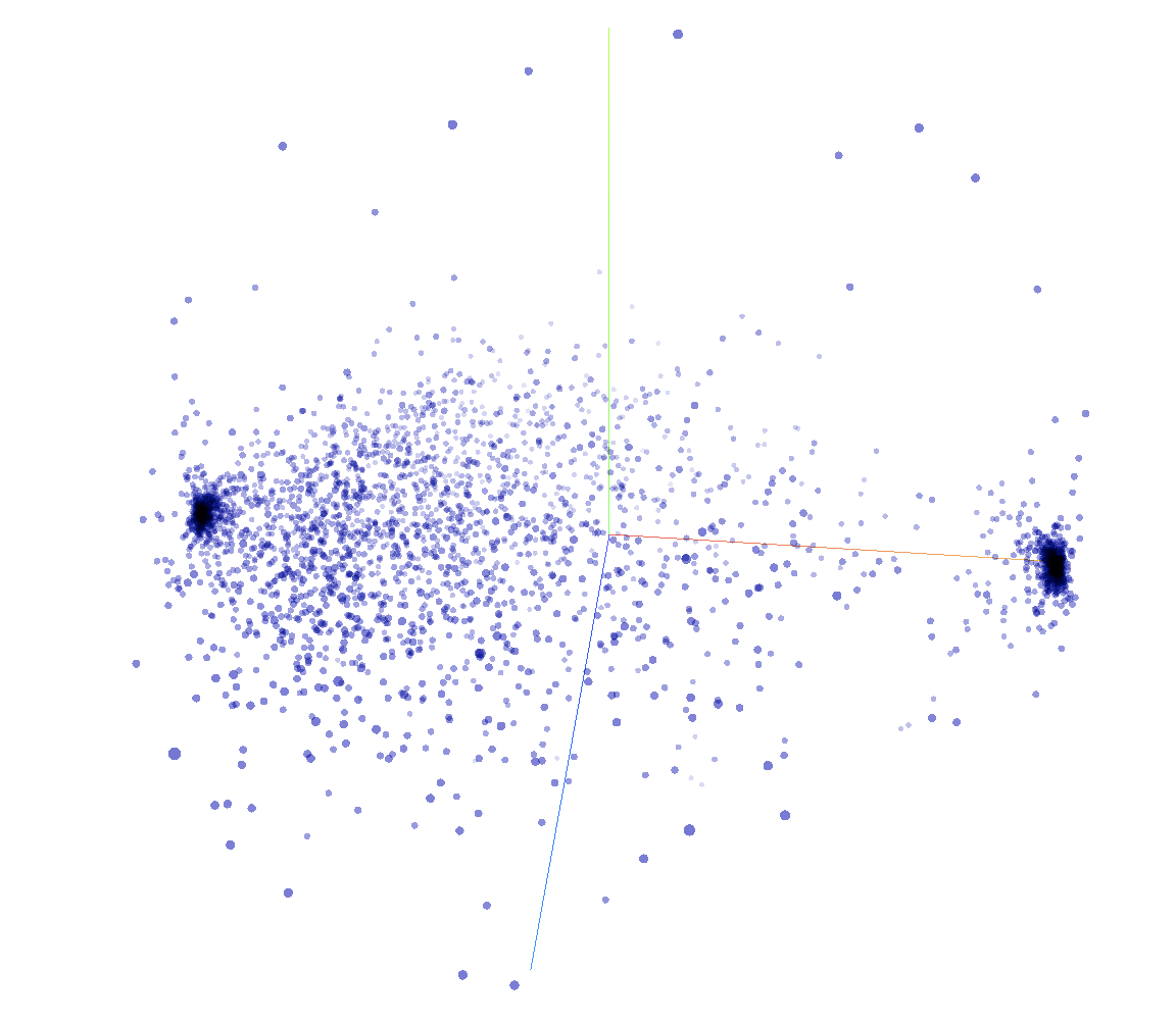
Figure 3: Projecting 50-dimensional embeddings obtained by training a simple neural network without SSE (Left), and with SSE-Graph (Center) , SSE-SE (Right) into 3D space using PCA.

3.2 Simplified SSE with Complete Graph: SSE-SE

One clear limitation of applying the SSE-Graph is that not every dataset comes with good-quality knowledge graphs on embeddings. For those cases, we could assume there is a complete graph over all embeddings so there is a small transition probability between every pair of different embeddings:

$$p(j,k|\Phi)=\frac{p_{0}}{N-1},\quad\forall 1\leq k\neq j\leq N,$$ (5)

where $N$ is the size of the embedding table. The SGD procedure in Algorithm 1 can still be applied and we call this algorithm SSE-SE (Stochastic Shared Embeddings - Simple and Easy). It is worth noting that SSE-Graph and SSE-SE are applied to embeddings associated with not only input $x_{i}$ but also those with output $y_{i}$. Unless there are considerably many more embeddings than data points and model is significantly overfitting, normally $p_{0}=0.01$ gives reasonably good results.

Interestingly, we found that the SSE-SE framework is related to several techniques used in practice. For example, BERT pre-training unintentionally applied a method similar to SSE-SE to input $x_{i}$ by replacing the masked word with a random word. This would implicitly introduce an SSE layer for input $x_{i}$ in Figure 1, because now embeddings associated with input $x_{i}$ be stochastically mapped according to (5). The main difference between this and SSE-SE is that it merely augments the input once, while SSE introduces randomization at every iteration, and we can also accommodate label embeddings. In experimental Section 4.4, we will show that SSE-SE would improve original BERT pre-training procedure as well as fine-tuning procedure.

3.3 Theoretical Guarantees

We explain why SSE can reduce the variance of estimators and thus leads to better generalization performance. For simplicity, we consider the SSE-graph objective (2) where there is no transition associated with the label $y_{i}$, and only the embeddings associated with the input $x_{i}$ undergo a transition. When this is the case, we can think of the loss as a function of the $x_{i}$ embedding and the label, $\ell(\mathbf{E}[\mathbf{j}^{i}],y_{i};\Theta)$. We take this approach because it is more straightforward to compare our resulting theory to existing excess risk bounds.

The SSE objective in the case of only input transitions can be written as,

$$S_{n}(\Theta)=\sum_{i}\sum_{\mathbf{k}}p(\mathbf{j}^{i},\mathbf{k})\cdot\ell(\mathbf{E}[\mathbf{k}],y_{i}|\Theta),$$ (6)

and there may be some constraint on $\Theta$. Let $\hat{\Theta}$ denote the minimizer of $S_{n}$ subject to this constraint. We will show in the subsequent theory that minimizing $S_{n}$ will get us close to a minimizer of $S(\Theta)=\mathbb{E}S_{n}(\Theta)$, and that under some conditions this will get us close to the Bayes risk. We will use the standard definitions of empirical and true risk, $R_{n}(\Theta)=\sum_{i}\ell(x_{i},y_{i}|\Theta)$ and $R(\Theta)=\mathbb{E}R_{n}(\Theta)$.

Our results depend on the following decomposition of the risk. By optimality of $\hat{\Theta}$,

$$R(\hat{\Theta})=S_{n}(\hat{\Theta})+[R(\hat{\Theta})-S(\hat{\Theta})]+[S(\hat{\Theta})-S_{n}(\hat{\Theta})]\leq S_{n}(\Theta^{\ast})+B(\hat{\Theta})+\mathcal{E}(\hat{\Theta})$$ (7)

where $B(\Theta)=|R(\Theta)-S(\Theta)|$, and $E(\Theta)=|S(\Theta)-S_{n}(\Theta)|$. We can think of $B(\Theta)$ as representing the bias due to SSE, and $E(\Theta)$ as an SSE form of excess risk. Then by another application of similar bounds,

$$R(\hat{\Theta})\leq R(\Theta^{\ast})+B(\hat{\Theta})+B(\Theta^{\ast})+E(\hat{\Theta})+E(\Theta^{\ast}).$$ (8)

The high level idea behind the following results is that when the SSE protocol reflects the underlying distribution of the data, then the bias term $B(\Theta)$ is small, and if the SSE transitions are well mixing then the SSE excess risk $E(\Theta)$ will be of smaller order than the standard Rademacher complexity. This will result in a small excess risk.

Theorem 1.

Consider SSE-graph with only input transitions. Let $L(\mathbf{E}[\mathbf{j}^{i}])=\mathbb{E}_{Y|X=x^{i}}\ell(\mathbf{E}[\mathbf{j}^{i}],Y|\Theta)$ be the expected loss conditional on input $x^{i}$ and $e(\mathbf{E}[\mathbf{j}^{i}],y|\Theta)=\ell(\mathbf{E}[\mathbf{j}^{i}],y|\Theta)-L(\mathbf{E}[\mathbf{j}^{i}]|\Theta)$ be the residual loss. Define the conditional and residual SSE empirical Rademacher complexities to be

$$\rho_{L,n}=\mathbb{E}_{\sigma}\sup_{\Theta}\left|\sum_{i}\sigma_{i}\sum_{\mathbf{k}}p(\mathbf{j}^{i},\mathbf{k})\cdot L(\mathbf{E}[\mathbf{k}]|\Theta)\right|,$$ (9)

$$\rho_{e,n}=\mathbb{E}_{\sigma}\sup_{\Theta}\left|\sum_{i}\sigma_{i}\sum_{\mathbf{k}}p(\mathbf{j}^{i},\mathbf{k})\cdot e(\mathbf{E}[\mathbf{k}],y_{i};\Theta)\right|,$$ (10)

respectively where $\sigma$ is a Rademacher $\pm 1$ random vectors in $\mathbb{R}^{n}$. Then we can decompose the SSE empirical risk into

$$\mathbb{E}\sup_{\Theta}|S_{n}(\Theta)-S(\Theta)|\leq 2\mathbb{E}[\rho_{L,n}+\rho_{e,n}].$$ (11)

Remark 1.

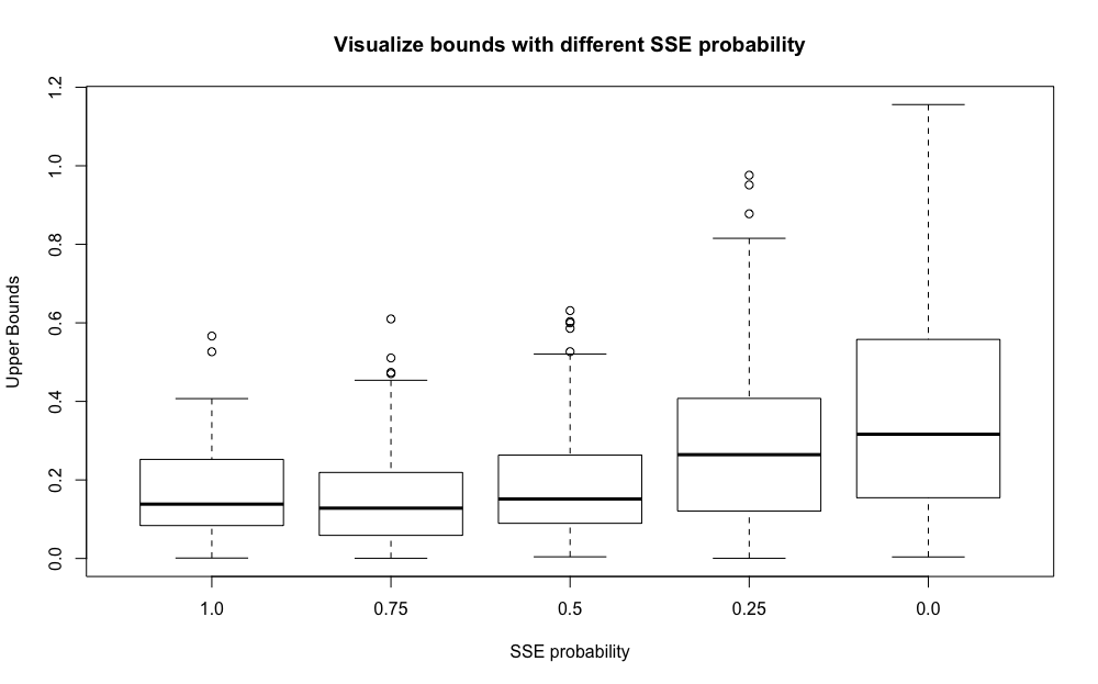
Figure 5: Simulation of a bound on $\rho_{L,n}$ for the movielens1M dataset. Throughout the simulation, $L$ is replaced with $\ell$ (which will bound $\rho_{L,n}$ by Jensen’s inequality). The SSE probability parameter dictates the probability of transitioning. When this is $0$ (box plot on the right), the distribution is that of the samples from the standard Rademacher complexity (without the sup and expectation). As we increase the transition probability, the values for $\rho_{L,n}$ get smaller.

The transition probabilities in (9), (10) act to smooth the empirical Rademacher complexity. To see this, notice that we can write the inner term of (9) as $(P\sigma)^{\top}L$, where we have vectorized $\sigma_{i},L(x_{i};\Theta)$ and formed the transition matrix $P$. Transition matrices are contractive and will induce dependencies between the Rademacher random variables, thereby stochastically reducing the supremum. In the case of no label noise, namely that $Y|X$ is a point mass, $e(x,y;\Theta)=0$, and $\rho_{e,n}=0$. The use of $L$ as opposed to the losses, $\ell$, will also make $\rho_{L,n}$ of smaller order than the standard empirical Rademacher complexity. We demonstrate this with a partial simulation of $\rho_{L,n}$ on the Movielens1m dataset in Figure 5 of the Appendix.

Theorem 2.

Let the SSE-bias be defined as

$$\mathcal{B}=\sup_{\Theta}\left|\mathbb{E}\left[\sum_{i}\sum_{\mathbf{k}}p(\mathbf{j}^{i},\mathbf{k})\cdot\left(\ell(\mathbf{E}[\mathbf{k}],y_{i}|\Theta)-\ell(\mathbf{E}[\mathbf{j}^{i}],y_{i}|\Theta)\right)\right]\right|.$$

Suppose that $0\leq\ell(.,.;\Theta)\leq b$ for some $b>0$, then

$$\mathbb{P}\left\{R(\hat{\Theta})>R(\Theta^{*})+2\mathcal{B}+4\mathbb{E}[\rho_{L,n}+\rho_{e,n}]+\sqrt{n}u\right\}\leq e^{-\frac{u^{2}}{2b^{2}}}.$$

Table 1: Compare SSE-Graph and SSE-SE against ALS-MF with Graph Laplacian Regularization. The $p_{u}$ and $p_{i}$ are the SSE probabilities for user and item embedding tables respectively, as in (5). Definitions of $\rho_{u}$ and $\rho_{i}$ can be found in (3). Movielens10m does not have user graphs.

	Movielens1m					Movielens10m
Model	RMSE	$\rho_{u}$	$\rho_{i}$	$p_{u}$	$p_{i}$	RMSE	$\rho_{u}$	$\rho_{i}$	$p_{u}$	$p_{i}$
SGD-MF	1.0984	-	-	-	-	1.9490	-	-	-	-
Graph Laplacian + ALS-MF	1.0464	-	-	-	-	1.9755	-	-	-	-
SSE-Graph + SGD-MF	1.0145	500	200	0.005	0.005	1.9019	1	500	0.01	0.01
SSE-SE + SGD-MF	1.0150	1	1	0.005	0.005	1.9085	1	1	0.01	0.01

Table 2: SSE-SE outperforms Dropout for Neural Networks with One Hidden Layer such as Matrix Factorization Algorithm regardless of dimensionality we use. $p_{s}$ is the SSE probability for both user and item embedding tables and $p_{d}$ is the dropout probability.

	Douban			Movielens10m			Netflix
Model	RMSE	$p_{d}$	$p_{s}$	RMSE	$p_{d}$	$p_{s}$	RMSE	$p_{d}$	$p_{s}$
MF	0.7339	-	-	0.8851	-	-	0.8941	-	-
Dropout + MF	0.7296	0.1	-	0.8813	0.1	-	0.8897	0.1	-
SSE-SE + MF	0.7201	-	0.008	0.8715	-	0.008	0.8842	-	0.008
SSE-SE + Dropout + MF	0.7185	0.1	0.005	0.8678	0.1	0.005	0.8790	0.1	0.005

Table 3: SSE-SE outperforms dropout for Neural Networks with One Hidden Layer such as Bayesian Personalized Ranking Algorithm regardless of dimensionality we use. We report the metric precision for top $k$ recommendations as $P@k$.

	Movielens1m			Yahoo Music			Foursquare
Model	$P@1$	$P@5$	$P@10$	$P@1$	$P@5$	$P@10$	$P@1$	$P@5$	$P@10$
SQL-Rank (2018)	0.7369	0.6717	0.6183	0.4551	0.3614	0.3069	0.0583	0.0194	0.0170
BPR	0.6977	0.6568	0.6257	0.3971	0.3295	0.2806	0.0437	0.0189	0.0143
Dropout + BPR	0.7031	0.6548	0.6273	0.4080	0.3315	0.2847	0.0437	0.0184	0.0146
SSE-SE + BPR	0.7254	0.6813	0.6469	0.4297	0.3498	0.3005	0.0609	0.0262	0.0155

Remark 2.

The price for ‘smoothing’ the Rademacher complexity in Theorem 1 is that SSE may introduce a bias. This will be particularly prominent when the SSE transitions have little to do with the underlying distribution of $Y,X$. On the other extreme, suppose that $p(\mathbf{j},\mathbf{k})$ is non-zero over a neighborhood $\mathcal{N}_{\mathbf{j}}$ of $\mathbf{j}$, and that for data $x^{\prime},y^{\prime}$ with encoding $\mathbf{k}\in\mathcal{N}_{\mathbf{j}}$, $x^{\prime},y^{\prime}$ is identically distributed with $x_{i},y_{i}$, then $\mathcal{B}=0$. In all likelihood, the SSE transition probabilities will not be supported over neighborhoods of iid random pairs, but with a well chosen SSE protocol the neighborhoods contain approximately iid pairs and $\mathcal{B}$ is small.

4 Experiments

We have conducted extensive experiments on 6 tasks, including 3 recommendation tasks (explicit feedback, implicit feedback and sequential recommendation) and 3 NLP tasks (neural machine translation, BERT pre-training, and BERT fine-tuning for sentiment classification) and found that our proposed SSE can effectively improve generalization performances on a wide variety of tasks. Note that the details about datasets and parameter settings can be found in the appendix.

4.1 Neural Networks with One Hidden Layer (Matrix Factorization and BPR)

Matrix Factorization Algorithm (MF) [17] and Bayesian Personalized Ranking Algorithm (BPR) [25] can be viewed as neural networks with one hidden layer (latent features) and are quite popular in recommendation tasks. MF uses the squared loss designed for explicit feedback data while BPR uses the pairwise ranking loss designed for implicit feedback data.

First, we conduct experiments on two explicit feedback datasets: Movielens1m and Movielens10m. For these datasets, we can construct graphs based on actors/actresses starring the movies. We compare SSE-graph and the popular Graph Laplacian Regularization (GLR) method [24] in Table 1. The results show that SSE-graph consistently outperforms GLR. This indicates that our SSE-Graph has greater potentials over graph Laplacian regularization as we do not explicitly penalize the distances across embeddings, but rather we implicitly penalize the effects of similar embeddings on the loss. Furthermore, we show that even without existing knowledge graphs of embeddings, our SSE-SE performs only slightly worse than SSE-Graph but still much better than GLR and MF.

In general, SSE-SE is a good alternative when graph information is not available. We then show that our proposed SSE-SE can be used together with standard regularization techniques such as dropout and weight decay to improve recommendation results regardless of the loss functions and dimensionality of embeddings. This is evident in Table 2 and Table 3. With the help of SSE-SE, BPR can perform better than the state-of-art listwise approach SQL-Rank [32] in most cases. We include the optimal SSE parameters in the table for references and leave out other experiment details to the appendix. In the rest of the paper, we would mostly focus on SSE-SE as we do not have high-quality graphs of embeddings on most datasets.

Table 4: SSE-SE has two tuning parameters: probability $p_{x}$ to replace embeddings associated with input $x_{i}$ and probability $p_{y}$ to replace embeddings associated with output $y_{i}$. We use the dropout probability of $0.1$, weight decay of $1e^{-5}$, and learning rate of $1e^{-3}$ for all experiments.

	Movielens1m		Dimension	$\#$ of Blocks	SSE-SE Parameters
Model	NDCG$@10$	Hit Ratio$@10$	$d$	$b$	$p_{x}$	$p_{y}$
SASRec	0.5941	0.8182	100	2	-	-
SASRec	0.5996	0.8272	100	6	-	-
SSE-SE + SASRec	0.6092	0.8250	100	2	0.1	0
SSE-SE + SASRec	0.6085	0.8293	100	2	0	0.1
SSE-SE + SASRec	0.6200	0.8315	100	2	0.1	0.1
SSE-SE + SASRec	0.6265	0.8364	100	6	0.1	0.1

4.2 Transformer Encoder Model for Sequential Recommendation

SASRec [11] is the state-of-the-arts algorithm for sequential recommendation task. It applies the transformer model [30], where a sequence of items purchased by a user can be viewed as a sentence in transformer, and next item prediction is equivalent to next word prediction in the language model. In Table 4, we perform SSE-SE on input embeddings ($p_{x}=0.1$, $p_{y}=0$), output embeddings ($p_{x}=0.1$, $p_{y}=0$) and both embeddings ($p_{x}=p_{y}=0.1$), and observe that all of them significantly improve over state-of-the-art SASRec ($p_{x}=p_{y}=0$). The regularization effects of SSE-SE is even more obvious when we increase the number of self-attention blocks from 2 to 6, as this will lead to a more sophisticated model with many more parameters. This leads to the model overfitting terribly even with dropout and weight decay. We can see in Table 4 that when both methods use dropout and weight decay, SSE-SE + SASRec is doing much better than SASRec without SSE-SE.

Table 5: Our proposed SSE-SE helps the Transformer achieve better BLEU scores on English-to-German in 10 out of 11 newstest data between 2008 and 2018.

	Test BLEU
Model	2008	2009	2010	2011	2012	2013	2014	2015	2016	2017	2018
Transformer	21.0	20.7	22.7	20.6	20.6	25.3	26.2	28.4	32.1	27.2	38.8
SSE-SE + Transformer	21.4	21.1	23.0	21.0	20.8	25.2	27.2	29.2	33.1	27.9	39.9

4.3 Neural Machine Translation

We use the transformer model [30] as the backbone for our experiments. The baseline model is the standard 6-layer transformer architecture and we apply SSE-SE to both encoder, and decoder by replacing corresponding vocabularies’ embeddings in the source and target sentences. We trained on the standard WMT 2014 English to German dataset which consists of roughly 4.5 million parallel sentence pairs and tested on WMT 2008 to 2018 news-test sets. We use the OpenNMT implementation in our experiments. We use the same dropout rate of 0.1 and label smoothing value of 0.1 for the baseline model and our SSE-enhanced model. The only difference between the two models is whether or not we use our proposed SSE-SE with $p_{0}=0.01$ in (5) for both encoder and decoder embedding layers. We evaluate both models’ performances on the test datasets using BLEU scores [21].

We summarize our results in Table 5 and find that SSE-SE helps improving accuracy and BLEU scores on both dev and test sets in 10 out of 11 years from 2008 to 2018. In particular, on the last 5 years’ test sets from 2014 to 2018, the transformer model with SSE-SE improves BLEU scores by 0.92 on average when compared to the baseline model without SSE-SE.

4.4 BERT for Sentiment Classification

BERT’s model architecture [3] is a multi-layer bidirectional Transformer encoder based on the Transformer model in neural machine translation. Despite SSE-SE can be used for both pre-training and fine-tuning stages of BERT, we want to mainly focus on pre-training as fine-tuning bears more similarity to the previous section. We use SSE probability of 0.015 for embeddings (one-hot encodings) associated with labels and SSE probability of 0.015 for embeddings (word-piece embeddings) associated with inputs. One thing worth noting is that even in the original BERT model’s pre-training stage, SSE-SE is already implicitly used for token embeddings. In original BERT model, the authors masked 15% of words for a maximum of 80 words in sequences of maximum length of 512 and 10% of the time replaced the [mask] token with a random token. That is roughly equivalent to SSE probability of 0.015 for replacing input word-piece embeddings.

We continue to pre-train Google pre-trained BERT model on our crawled IMDB movie reviews with and without SSE-SE and compare downstream tasks performances. In Table 6, we find that SSE-SE pre-trained BERT base model helps us achieve the state-of-the-art results for the IMDB sentiment classification task, which is better than the previous best in [9]. We report test set accuracy of 0.9542 after fine-tuning for one epoch only. For the similar SST-2 sentiment classification task in Table 7, we also find that SSE-SE can improve BERT pre-trains better. Our SSE-SE pre-trained model achieves 94.3% accuracy on SST-2 test set after 3 epochs of fine-tuning while the standard pre-trained BERT model only reports 93.8 after fine-tuning. Furthermore, we show that SSE-SE with SSE probability 0.01 can also improve dev and test accuracy in the fine-tuning stage. If we are using SSE-SE for both pre-training and fine-tuning stage of the BERT base model, we can achieve 94.5% accuracy on the SST-2 test set, approaching the 94.9% accuracy by the BERT large model. We are optimistic that our SSE-SE can be applied to BERT large model as well in the future.

Table 6: Our proposed SSE-SE applied in the pre-training stage on our crawled IMDB data improves the generalization ability of pre-trained IMDB model and helps the BERT-Base model outperform current SOTA results on the IMDB Sentiment Task after fine-tuning.

	IMDB Test Set
Model	AUC	Accuracy	F1 Score
ULMFiT [9]	-	0.9540	-
Google Pre-trained Model + Fine-tuning	0.9415	0.9415	0.9419
Pre-training + Fine-tuning	0.9518	0.9518	0.9523
(SSE-SE + Pre-training) + Fine-tuning	0.9542	0.9542	0.9545

Table 7: SSE-SE pre-trained BERT-Base models on IMDB datasets turn out working better on the new unseen SST-2 Task as well.

	SST-2 Dev Set			SST-2 Test Set
Model	AUC	Accuracy	F1 Score	Accuracy (%)
Google Pre-trained + Fine-tuning	0.9230	0.9232	0.9253	93.6
Pre-training + Fine-tuning	0.9265	0.9266	0.9281	93.8
(SSE-SE + Pre-training) + Fine-tuning	0.9276	0.9278	0.9295	94.3
(SSE-SE + Pre-training) + (SSE-SE + Fine-tuning)	0.9323	0.9323	0.9336	94.5

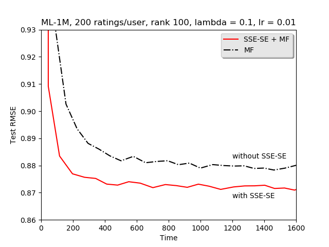
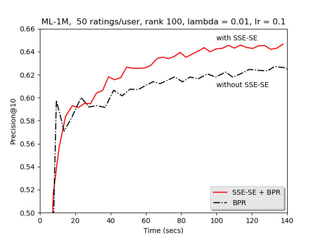
Figure 4: Compare Training Speed of Simple Neural Networks with One Hidden Layer, i.e. MF and BPR, with and without SSE-SE.

4.5 Speed and Convergence Comparisons.

In Figure 4, it is clear to see that our one-hidden-layer neural networks with SSE-SE are achieving much better generalization results than their respective standalone versions. One can also easily spot that SSE-version algorithms converge at much faster speeds with the same learning rate.

5 Conclusion

We have proposed Stochastic Shared Embeddings, which is a data-driven approach to regularization, that stands in contrast to brute force regularization such as Laplacian and ridge regularization. Our theory is a first step towards explaining the regularization effect of SSE, particularly, by ‘smoothing’ the Rademacher complexity. The extensive experimentation demonstrates that SSE can be fruitfully integrated into existing deep learning applications.

Acknowledgement. Hsieh acknowledges the support of NSF IIS-1719097, Intel faculty award, Google Cloud and Nvidia.

6 Appendix

For experiments in Section 4.1, we use Julia and C++ to implement SGD. For experiments in Section 4.2, and Section 4.4, we use Tensorflow and SGD/Adam Optimizer. For experiments in Section 4.3, we use Pytorch and Adam with noam decay scheme and warm-up. We find that none of these choices affect the strong empirical results supporting the effectiveness of our proposed methods, especially the SSE-SE. In any deep learning frameworks, we can introduce stochasticity to the original embedding look-up behaviors and easily implement SSE-Layer in Figure 1 as a custom operator.

6.1 Neural Networks with One Hidden Layer

To run SSE-Graph, we need to construct good-quality knowledge graphs on embeddings. We managed to match movies in Movielens1m and Movielens10m datasets to IMDB websites, therefore we can extract plentiful information for each movie, such as the cast of the movies, user reviews and so on. For simplicity reason, we construct the knowledge graph on item-side embeddings using the cast of movies. Two items are connected by an edge when they share one or more actors/actresses. For user side, we do not have good quality graphs: we are only able to create a graph on users in Movielens1m dataset based on their age groups but we do not have any side information on users in Movielens10m dataset. When running experiments, we do a parameter sweep for weight decay parameter and then fix it before tuning the parameters for SSE-Graph and SSE-SE. We utilize different $\rho$ and $p$ for user and item embedding tables respectively. The optimal parameters are stated in Table 1 and Table 2. We use the learning rate of 0.01 in all SGD experiments.

In the first leg of experiments, we examine users with fewer than 60 ratings in Movielens1m and Movielens10m datasets. In this scenario, the graph should carry higher importance. One can easily see from Table 1 that without using graph information, our proposed SSE-SE is the best performing matrix factorization algorithms among all methods, including popular ALS-MF and SGD-MF in terms of RMSE. With Graph information, our proposed SSE-Graph is performing significantly better than the Graph Laplacian Regularized Matrix Factorization method. This indicates that our SSE-Graph has great potentials over Graph Laplacian Regularization as we do not explicitly penalize the distances across embeddings but rather we implicitly penalize the effects of similar embeddings on the loss.

In the second leg of experiments, we remove the constraints on the maximum number of ratings per user. We want to show that SSE-SE can be a good alternative when graph information is not available. We follow the same procedures in [31, 32]. In Table 2, we can see that SSE-SE can be used with dropout to achieve the smallest RMSE across Douban, Movielens10m, and Netflix datasets. In Table 3, one can see that SSE-SE is more effective than dropout in this case and can perform better than STOA listwise approach SQL-Rank [32] on 2 datasets out of 3.

In Table 2, SSE-SE has two tuning parameters: probability $p_{u}$ to replace embeddings associated with user-side embeddings and probability $p_{i}$ to replace embeddings associated with item side embeddings because there are two embedding tables. But here for simplicity, we use one tuning parameter $p_{s}=p_{u}=p_{i}$. We use dropout probability of $p_{d}$, dimension of user/item embeddings $d$, weight decay of $\lambda$ and learning rate of $0.01$ for all experiments, with the exception that the learning rate is reduced to $0.005$ when both SSE-SE and Dropout are applied. For Douban dataset, we use $d=10,\lambda=0.08$. For Movielens10m and Netflix dataset, we use $d=50,\lambda=0.1$.

6.2 Neural Machine Translation

We use the transformer model [30] as the backbone for our experiments. The control group is the standard transformer encoder-decoder architecture with self-attention. In the experiment group, we apply SSE-SE towards both encoder and decoder by replacing corresponding vocabularies’ embeddings in the source and target sentences. We trained on the standard WMT 2014 English to German dataset which consists of roughly 4.5 million parallel sentence pairs and tested on WMT 2008 to 2018 news-test sets. Sentences were encoded into 32,000 tokens using a byte-pair encoding. We use the SentencePiece, OpenNMT and SacreBLEU implementations in our experiments. We trained the 6-layer transformer base model on a single machine with 4 NVIDIA V100 GPUs for 20,000 steps. We use the same dropout rate of 0.1 and label smoothing value of 0.1 for the baseline model and our SSE-enhanced model. Both models have dimensionality of embeddings as $d=512$. When decoding, we use beam search with the beam size of 4 and length penalty of 0.6 and replace unknown words using attention. For both models, we average last 5 checkpoints (we save checkpoints every 10,000 steps) and evaluate the model’s performances on the test datasets using BLEU scores. The only difference between the two models is whether or not we use our proposed SSE-SE with $p=0.01$ in Equation 5 for both encoder and decoder embedding layers.

6.3 BERT

In the first leg of experiments, we crawled one million user reviews data from IMDB and pre-trained the BERT-Base model (12 blocks) for $500,000$ steps using sequences of maximum length 512 and batch size of 8, learning rates of $2e^{-5}$ for both models using one NVIDIA V100 GPU. Then we pre-trained on a mixture of our crawled reviews and reviews in IMDB sentiment classification tasks (250K reviews in train and 250K reviews in test) for another $200,000$ steps before training for another $100,000$ steps for the reviews in IMDB sentiment classification task only. In total, both models are pre-trained on the same datasets for $800,000$ steps with the only difference being our model utilizes SSE-SE. In the second leg of experiments, we fine-tuned the two models obtained in the first-leg experiments on two sentiment classification tasks: IMDB sentiment classification task and SST-2 sentiment classification task. The goal of pre-training on IMDB dataset but fine-tuning for SST-2 task is to explore whether SSE-SE can play a role in transfer learning.

The results are summarized in Table 6 for IMDB sentiment task. In experiments, we use maximum sequence length of 512, learning rate of $2e^{-5}$, dropout probability of $0.1$ and we run fine-tuning for 1 epoch for the two pre-trained models we obtained before. For the Google pre-trained BERT-base model, we find that we need to run a minimum of 2 epochs. This shows that pre-training can speed up the fine-tuning. We find that Google pre-trained model performs worst in accuracy because it was only pre-trained on Wikipedia and books corpus while ours have seen many additional user reviews. We also find that SSE-SE pre-trained model can achieve accuracy of 0.9542 after fine-tuning for one epoch only. On the contrast, the accuracy is only 0.9518 without SSE-SE for embeddings associated with output $y_{i}$.

For the SST-2 task, we use maximum sequence length of 128, learning rate of $2e^{-5}$, dropout probability of 0.1 and we run fine-tuning for 3 epochs for all 3 models in Table 7. We report AUC, accuracy and F1 score for dev data. For test results, we submitted our predictions to Glue website for the official evaluation. We find that even in transfer learning, our SSE-SE pre-trained model still enjoys advantages over Google pre-trained model and our pre-trained model without SSE-SE. Our SSE-SE pre-trained model achieves 94.3% accuracy on SST-2 test set versus 93.6 and 93.8 respectively. If we are using SSE-SE for both pre-training and fine-tuning, we can achieve 94.5% accuracy on the SST-2 test set, which approaches the 94.9 score reported by the BERT-Large model. SSE probability of 0.01 is used for fine-tuning.

6.4 Proofs

Throughout this section, we will suppress the probability parameters, $p(.,.|\Phi)=p(.,.)$.

Proof of Theorem 1.

Consider the following variability term,

$$\sup_{\Theta}|S(\Theta)-S_{n}(\Theta)|.$$ (12)

Let us break the variability term into two components

$$\mathbb{E}_{X,Y}\sup_{\Theta}\left|S_{n}(\Theta)-\mathbb{E}_{Y|X}[S_{n}(\Theta)]\right|+\mathbb{E}_{X,Y}\sup_{\Theta}\left|\mathbb{E}_{Y|X}[S_{n}(\Theta)]-S(\Theta)\right|,$$

where $X,Y$ represent the random input and label. To control the first term, we introduce a ghost dataset $(x_{i},y_{i}^{\prime})$, where $y_{i}^{\prime}$ are independently and identically distributed according to $y_{i}|x_{i}$. Define

$$S^{\prime}_{n}(\Theta)=\sum_{i}\sum_{\mathbf{k}}p(\mathbf{j}^{i},\mathbf{k})\ell(\mathbf{E}[\mathbf{k}],y_{i}^{\prime}|\Theta)$$ (13)

be the empirical SSE risk with respect to this ghost dataset.

We will rewrite $\mathbb{E}_{Y|X}[S_{n}(\Theta)]$ in terms of the ghost dataset and apply Jensen’s inequality and law of iterated conditional expectation:

$$\mathbb{E}\sup_{\Theta}\left|\mathbb{E}_{Y|X}[S_{n}(\Theta)]-S_{n}(\Theta)\right|$$ (14)

$$=\mathbb{E}\sup_{\Theta}\left|\mathbb{E}_{Y^{\prime}|X}\left[S^{\prime}_{n}(\Theta)-S_{n}(\Theta)\right]\right|$$ (15)

$$\leq\mathbb{E}\mathbb{E}_{Y^{\prime}|X}\left[\sup_{\Theta}\left|S^{\prime}_{n}(\Theta)-S_{n}(\Theta)\right|\right]$$ (16)

$$=\mathbb{E}\sup_{\Theta}\left|S^{\prime}_{n}(\Theta)-S_{n}(\Theta)\right|.$$ (17)

Notice that

$$S^{\prime}_{n}(\Theta)-S_{n}(\Theta)=\sum_{i}\sum_{\mathbf{k}}p(\mathbf{j}^{i},\mathbf{k})\left(\ell(\mathbf{E}[\mathbf{k}],y_{i}^{\prime}|\Theta)-\ell(\mathbf{E}[\mathbf{k}],y_{i}|\Theta)\right)$$

$$=\sum_{i}\sum_{\mathbf{k}}p(\mathbf{j}^{i},\mathbf{k})\left(e(\mathbf{E}[\mathbf{k}],y_{i}^{\prime}|\Theta)-e(\mathbf{E}[\mathbf{k}],y_{i}|\Theta)\right).$$

Because $y_{i},y_{i}^{\prime}|X$ are independent the term $(\sum_{\mathbf{k}}p(\mathbf{j}^{i},\mathbf{k})\left(e(\mathbf{E}[\mathbf{k}],y_{i}^{\prime}|\Theta)-e(\mathbf{E}[\mathbf{k}],y_{i}|\Theta)\right))_{i}$ is a vector of symmetric independent random variables. Thus its distribution is not effected by multiplication by arbitrary Rademacher vectors $\sigma_{i}\in\{-1,+1\}$.

$$\mathbb{E}\sup_{\Theta}\left|S^{\prime}_{n}(\Theta)-S_{n}(\Theta)\right|=\mathbb{E}\sup_{\Theta}\left|\sum_{i}\sigma_{i}\sum_{\mathbf{k}}p(\mathbf{j}^{i},\mathbf{k})\left(e(\mathbf{E}[\mathbf{k}],y_{i}^{\prime}|\Theta)-e(\mathbf{E}[\mathbf{k}],y_{i}|\Theta)\right)\right|.$$

But this is bounded by

$$2\mathbb{E}\mathbb{E}_{\sigma}\sup_{\Theta}\left|\sum_{i}\sigma_{i}\sum_{\mathbf{k}}p(\mathbf{j}^{i},\mathbf{k})e(\mathbf{E}[\mathbf{k}],y_{i}|\Theta)\right|.$$

For the second term,

$$\mathbb{E}\sup_{\Theta}\left|\mathbb{E}_{Y|X}[S_{n}(\Theta)]-S(\Theta)\right|$$

we will introduce a second ghost dataset $x_{i}^{\prime},y_{i}^{\prime}$ drawn iid to $x_{i},y_{i}$. Because we are augmenting the input then this results in a new ghost encoding $\mathbf{j}^{\prime i}$. Let

$$S^{\prime}_{n}(\Theta)=\sum_{i}\sum_{\mathbf{k}}p(\mathbf{j}^{\prime i},\mathbf{k})\ell(\mathbf{E}[\mathbf{k}],y_{i}^{\prime}|\Theta)$$ (18)

be the empirical risk with respect to this ghost dataset. Then we have that

$$S(\Theta)=\mathbb{E}_{X^{\prime}}\mathbb{E}_{Y^{\prime}|X^{\prime}}S_{n}^{\prime}(\Theta)$$

Thus,

$$\mathbb{E}\sup_{\Theta}\left|\mathbb{E}_{Y|X}[S_{n}(\Theta)]-S(\Theta)\right|$$ (19)

$$=\mathbb{E}\sup_{\Theta}\left|\mathbb{E}_{X^{\prime}}\left[E_{Y|X}[S_{n}(\Theta)]-E_{Y^{\prime}|X^{\prime}}[S^{\prime}_{n}(\Theta)]\right]\right|$$ (20)

$$\leq\mathbb{E}\mathbb{E}_{X^{\prime}}\left[\sup_{\Theta}\left|E_{Y|X}[S_{n}(\Theta)]-E_{Y^{\prime}|X^{\prime}}[S^{\prime}_{n}(\Theta)]\right|\right]$$ (21)

$$=\mathbb{E}\sup_{\Theta}\left|E_{Y|X}[S_{n}(\Theta)]-E_{Y^{\prime}|X^{\prime}}[S^{\prime}_{n}(\Theta)]\right|.$$ (22)

Notice that we may write,

$$E_{Y|X}[S_{n}(\Theta)]-E_{Y^{\prime}|X^{\prime}}[S^{\prime}_{n}(\Theta)]=\sum_{i}\sum_{\mathbf{k}}\left(p(\mathbf{j}^{i},\mathbf{k})-p(\mathbf{j}^{\prime i},\mathbf{k})\right)L(\mathbf{E}[\mathbf{k}]|\Theta)$$

Again we may introduce a second set of Rademacher random variables $\sigma^{\prime}_{i}$, which results in

$$\mathbb{E}\sup_{\Theta}\left|E_{Y|X}[S_{n}(\Theta)]-E_{Y^{\prime}|X^{\prime}}[S^{\prime}_{n}(\Theta)]\right|\leq 2\mathbb{E}\mathbb{E}_{\sigma^{\prime}}\sup_{\Theta}\left|\sum_{i}\sigma^{\prime}_{i}\sum_{\mathbf{k}}p(\mathbf{j}^{i},\mathbf{k})L(\mathbf{E}[\mathbf{k}]|\Theta)\right|.$$

And this is bounded by

$$2\mathbb{E}\mathbb{E}_{\sigma^{\prime}}\sup_{\Theta}\left|\sum_{i}\sigma^{\prime}_{i}\sum_{\mathbf{k}}p(\mathbf{j}^{i},\mathbf{k})L(\mathbf{E}[\mathbf{k}]|\Theta)\right|\leq 2\mathbb{E}\sup_{\Theta}\left|\sum_{i}\sigma^{\prime}_{i}\sum_{\mathbf{k}}p(\mathbf{j}^{i},\mathbf{k})\ell(\mathbf{E}[\mathbf{k}],y_{i}|\Theta)\right|$$

by Jensen’s inequality again. ∎

Proof of Theorem 2.

It is clear that $2\mathcal{B}\geq B(\hat{\Theta})+B(\Theta^{*})$. It remains to show our concentration inequality. Consider changing a single sample, $(x_{i},y_{i})$ to $(x_{i}^{\prime},y_{i}^{\prime})$, thus resulting in the SSE empirical risk, $S_{n,i}(\Theta)$. Thus,

$$S_{n}(\Theta)-S_{n,i}(\Theta)=\sum_{\mathbf{k}}p(\mathbf{j}^{i},\mathbf{k})\cdot\ell(\mathbf{E}[\mathbf{k}],y_{i}|\Theta)-\sum_{\mathbf{k}}p(\mathbf{j}^{\prime i},\mathbf{k})\cdot\ell(\mathbf{E}[\mathbf{k}],y_{i}^{\prime}|\Theta)$$

$$=\sum_{\mathbf{k}}p(\mathbf{j}^{i},\mathbf{k})\cdot\left(\ell(\mathbf{E}[\mathbf{k}],y_{i}|\Theta)-\ell(\mathbf{E}[\mathbf{k}],y_{i}^{\prime}|\Theta)\right)+\sum_{\mathbf{k}}\left(p(\mathbf{j}^{\prime i},\mathbf{k})-p(\mathbf{j}^{i},\mathbf{k})\right)\cdot\ell(\mathbf{E}[\mathbf{k}],y_{i}^{\prime}|\Theta)$$

$$\leq b\left(\sum_{\mathbf{k}}p(\mathbf{j}^{i},\mathbf{k})+\sum_{\mathbf{k}}p(\mathbf{j}^{\prime i},\mathbf{k})\right)\leq 2b.$$

Then the result follows from McDiarmid’s inequality.

∎

References

- Bennett et al. [2007] James Bennett, Stan Lanning, et al. The netflix prize. In Proceedings of KDD cup and workshop, volume 2007, page 35. New York, NY, USA., 2007.
- Cai et al. [2011] Deng Cai, Xiaofei He, Jiawei Han, and Thomas S Huang. Graph regularized nonnegative matrix factorization for data representation. IEEE transactions on pattern analysis and machine intelligence, 33(8):1548–1560, 2011.
- Devlin et al. [2018] Jacob Devlin, Ming-Wei Chang, Kenton Lee, and Kristina Toutanova. Bert: Pre-training of deep bidirectional transformers for language understanding. arXiv preprint arXiv:1810.04805, 2018.
- Duchi et al. [2011] John Duchi, Elad Hazan, and Yoram Singer. Adaptive subgradient methods for online learning and stochastic optimization. Journal of Machine Learning Research, 12(Jul):2121–2159, 2011.
- Goodfellow et al. [2016] Ian Goodfellow, Yoshua Bengio, Aaron Courville, and Yoshua Bengio. Deep learning, volume 1. MIT press Cambridge, 2016.
- He et al. [2017] Xiangnan He, Lizi Liao, Hanwang Zhang, Liqiang Nie, Xia Hu, and Tat-Seng Chua. Neural collaborative filtering. In Proceedings of the 26th International Conference on World Wide Web, pages 173–182. International World Wide Web Conferences Steering Committee, 2017.
- Hinton et al. [2012] Geoffrey E Hinton, Nitish Srivastava, Alex Krizhevsky, Ilya Sutskever, and Ruslan R Salakhutdinov. Improving neural networks by preventing co-adaptation of feature detectors. arXiv preprint arXiv:1207.0580, 2012.
- Hoerl and Kennard [1970] Arthur E Hoerl and Robert W Kennard. Ridge regression: Biased estimation for nonorthogonal problems. Technometrics, 12(1):55–67, 1970.
- Howard and Ruder [2018] Jeremy Howard and Sebastian Ruder. Universal language model fine-tuning for text classification. arXiv preprint arXiv:1801.06146, 2018.
- Hu et al. [2008] Yifan Hu, Yehuda Koren, and Chris Volinsky. Collaborative filtering for implicit feedback datasets. In ICDM, volume 8, pages 263–272. Citeseer, 2008.
- Kang and McAuley [2018] Wang-Cheng Kang and Julian McAuley. Self-attentive sequential recommendation. arXiv preprint arXiv:1808.09781, 2018.
- Kingma and Ba [2014] Diederik P Kingma and Jimmy Ba. Adam: A method for stochastic optimization. arXiv preprint arXiv:1412.6980, 2014.
- Krizhevsky et al. [2012] Alex Krizhevsky, Ilya Sutskever, and Geoffrey E Hinton. Imagenet classification with deep convolutional neural networks. In Advances in neural information processing systems, pages 1097–1105, 2012.
- Lehmann et al. [2015] Jens Lehmann, Robert Isele, Max Jakob, Anja Jentzsch, Dimitris Kontokostas, Pablo N Mendes, Sebastian Hellmann, Mohamed Morsey, Patrick Van Kleef, Sören Auer, et al. Dbpedia–a large-scale, multilingual knowledge base extracted from wikipedia. Semantic Web, 6(2):167–195, 2015.
- Mikolov et al. [2013] Tomas Mikolov, Ilya Sutskever, Kai Chen, Greg S Corrado, and Jeff Dean. Distributed representations of words and phrases and their compositionality. In Advances in neural information processing systems, pages 3111–3119, 2013.
- Miller [1995] George A Miller. Wordnet: a lexical database for english. Communications of the ACM, 38(11):39–41, 1995.
- Mnih and Salakhutdinov [2008] Andriy Mnih and Ruslan R Salakhutdinov. Probabilistic matrix factorization. In Advances in neural information processing systems, pages 1257–1264, 2008.
- Nowlan and Hinton [1992] Steven J Nowlan and Geoffrey E Hinton. Simplifying neural networks by soft weight-sharing. Neural computation, 4(4):473–493, 1992.
- Pascanu et al. [2013] Razvan Pascanu, Tomas Mikolov, and Yoshua Bengio. On the difficulty of training recurrent neural networks. In International Conference on Machine Learning, pages 1310–1318, 2013.
- Pennington et al. [2014] Jeffrey Pennington, Richard Socher, and Christopher Manning. Glove: Global vectors for word representation. In Proceedings of the 2014 conference on empirical methods in natural language processing (EMNLP), pages 1532–1543, 2014.
- Post [2018] Matt Post. A call for clarity in reporting BLEU scores. In Proceedings of the Third Conference on Machine Translation: Research Papers, pages 186–191, Belgium, Brussels, October 2018. Association for Computational Linguistics. URL https://www.aclweb.org/anthology/W18-6319.
- Radford et al. [2018] Alec Radford, Karthik Narasimhan, Tim Salimans, and Ilya Sutskever. Improving language understanding by generative pre-training. URL https://s3-us-west-2. amazonaws. com/openai-assets/research-covers/languageunsupervised/language understanding paper. pdf, 2018.
- Radford et al. [2019] Alec Radford, Jeffrey Wu, Rewon Child, David Luan, Dario Amodei, and Ilya Sutskever. Language models are unsupervised multitask learners. URL https://openai. com/blog/better-language-models, 2019.
- Rao et al. [2015] Nikhil Rao, Hsiang-Fu Yu, Pradeep K Ravikumar, and Inderjit S Dhillon. Collaborative filtering with graph information: Consistency and scalable methods. In Advances in neural information processing systems, pages 2107–2115, 2015.
- Rendle et al. [2009] Steffen Rendle, Christoph Freudenthaler, Zeno Gantner, and Lars Schmidt-Thieme. Bpr: Bayesian personalized ranking from implicit feedback. In Proceedings of the twenty-fifth conference on uncertainty in artificial intelligence, pages 452–461. AUAI Press, 2009.
- Srebro et al. [2005] Nathan Srebro, Jason Rennie, and Tommi S Jaakkola. Maximum-margin matrix factorization. In Advances in neural information processing systems, pages 1329–1336, 2005.
- Srivastava et al. [2014] Nitish Srivastava, Geoffrey Hinton, Alex Krizhevsky, Ilya Sutskever, and Ruslan Salakhutdinov. Dropout: a simple way to prevent neural networks from overfitting. The Journal of Machine Learning Research, 15(1):1929–1958, 2014.
- Szegedy et al. [2016] Christian Szegedy, Vincent Vanhoucke, Sergey Ioffe, Jon Shlens, and Zbigniew Wojna. Rethinking the inception architecture for computer vision. In Proceedings of the IEEE conference on computer vision and pattern recognition, pages 2818–2826, 2016.
- Tibshirani [1996] Robert Tibshirani. Regression shrinkage and selection via the lasso. Journal of the Royal Statistical Society. Series B (Methodological), pages 267–288, 1996.
- Vaswani et al. [2017] Ashish Vaswani, Noam Shazeer, Niki Parmar, Jakob Uszkoreit, Llion Jones, Aidan N Gomez, Łukasz Kaiser, and Illia Polosukhin. Attention is all you need. In Advances in Neural Information Processing Systems, pages 5998–6008, 2017.
- Wu et al. [2017] Liwei Wu, Cho-Jui Hsieh, and James Sharpnack. Large-scale collaborative ranking in near-linear time. In Proceedings of the 23rd ACM SIGKDD International Conference on Knowledge Discovery and Data Mining, pages 515–524. ACM, 2017.
- Wu et al. [2018] Liwei Wu, Cho-Jui Hsieh, and James Sharpnack. Sql-rank: A listwise approach to collaborative ranking. In Proceedings of Machine Learning Research (35th International Conference on Machine Learning), volume 80, 2018.