Exposure Bias versus Self-Recovery:
Are Distortions Really Incremental for Autoregressive Text Generation?

Abstract

Exposure bias has been regarded as a central problem for auto-regressive language models (LM). It claims that teacher forcing would cause the test-time generation to be incrementally distorted due to the training-generation discrepancy. Although a lot of algorithms have been proposed to avoid teacher forcing and therefore alleviate exposure bias, there is little work showing how serious the exposure bias problem actually is. In this work, we focus on the task of open-ended language generation, propose metrics to quantify the impact of exposure bias in the aspects of quality, diversity, and consistency. Our key intuition is that if we feed ground-truth data prefixes (instead of prefixes generated by the model itself) into the model and ask it to continue the generation, the performance should become much better because the training-generation discrepancy in the prefix is removed. Both automatic and human evaluations are conducted in our experiments. On the contrary to the popular belief in exposure bias, we find that the the distortion induced by the prefix discrepancy is limited, and does not seem to be incremental during the generation. Moreover, our analysis reveals an interesting self-recovery ability of the LM, which we hypothesize to be countering the harmful effects from exposure bias.

1 Introduction

Language model (LM) has been a central module for natural language generation (NLG) tasks (Young et al., 2017) such as open-ended language generation (Radford et al., 2018; Brown et al., 2020), machine translation (Wu et al., 2017), dialogue response generation (Li et al., 2017), image captioning (Lin et al., 2014), etc. For decades, maximum likelihood estimation (MLE) has been the most widely used objective for LM training. However, there is a popular belief in the natural language processing (NLP) community that standard MLE training suffers from the exposure bias problem which leads to an incremental performance degradation during test-time generation.

The claim of the exposure bias problem (Bengio et al., 2015; Ranzato et al., 2016) is originated from the following discrepancy between MLE training and test-time generation for auto-regressive language models: During training, the model is trained to predict the next word conditioned on prefix (or history) words sampled from the ground-truth data distribution; While during generation, the model generates words conditioned on prefix sequences sampled from the model itself. Due to the exposure to real data during training, the language model could potentially be biased to only perform well with data prefixes. Therefore, it is claimed (and widely believed among researchers) that during generation the errors could accumulate along the generated sequence, and the distribution generated by the model would be incrementally distorted. The forced exposure to ground-truth data during training is also referred to as teacher forcing.

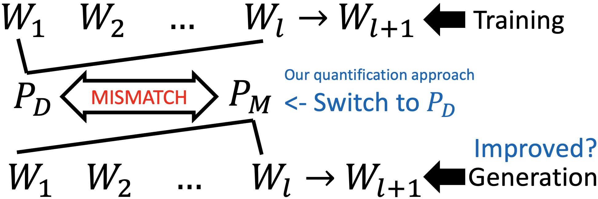
Figure 1: An illustration of the training-generation discrepancy and our key intuition for verifying exposure bias (in blue): During generation, if we feed ground-truth data prefixes (from $P_{D}$) instead of the model’s own samples ($P_{M}$), the generation performance should be better because the prefix discrepancy is removed.

To avoid teacher forcing, many training algorithms (Bengio et al., 2015; Lamb et al., 2016; Ranzato et al., 2016; Yu et al., 2016; Zhu et al., 2018; Lu et al., 2018; Lin et al., 2017; Guo et al., 2017; Rajeswar et al., 2017; Wiseman and Rush, 2016; Nie et al., 2019; Shi et al., 2018; de Masson d’Autume et al., 2019; Rennie et al., 2016; Feng et al., 2021) have been proposed as alternatives to MLE training for text generation. Many of these works utilize techniques from generative adversarial networks (GANs) (Goodfellow et al., 2014) or reinforcement learning (RL) (Sutton and Barto, 1998). In this work, we refer to these algorithms as non-MLE methods or text GANs.

With the huge research efforts devoted to alleviate exposure bias, interestingly, the existence or significance of exposure bias is much less studied. Interestingly, despite the criticism, MLE (teacher forcing) has remained to be the dominant objective for LM training (Radford et al., 2018; Keskar et al., 2019; Brown et al., 2020). On the other hand, non-MLE training methods are still struggling to outperform the MLE baseline (Caccia et al., 2018; de Masson d’Autume et al., 2019). These developments lead us to question: Is exposure bias truly a serious problem for MLE training?

In this work we seek a direct answer to the above question. Here we briefly summarize our contributions: We design and experiment with various metrics to quantify the impact from exposure bias. On the contrary to our expectation, our measurements consistently show that removing the prefix discrepancy only brings limited gain, and the incremental distortion is not observed. Moreover, our analysis reveals an interesting self-recovery ability of the LM, which we hypothesize to be countering the harmful effects from exposure bias.

2 Related Works

We first clarify that “Whether exposure bias is serious for MLE training?" and “Whether new non-MLE algorithms improve generation performance?" are two related but different questions, and our work has a clear focus on the first question. Despite the large body of works (listed in Section 1) devoted to alleviate exposure bias, its actual impact has rarely been systematically studied or validated in a direct and principled way. Zhang et al. (2019) attempts to measure the gain from alleviating exposure bias, by counting the ground truth words whose probabilities in the predicted distributions produced by their proposed model are greater than those from the baseline model. However, it is unclear how this experiment can be linked to exposure bias. Schmidt (2019) provides valuable discussions around the claim of exposure bias, but they did not propose an operational definition or metric. Xu et al. (2019) attempts to measure exposure bias by comparing the model’s performance on seen (training) data and unseen (test) data. However, this methodology is more about the generalization gap, instead of exposure bias. Finally, Wang and Sennrich (2020) discusses the potential link between exposure bias and hallucination in the context of machine translation.

In a relevant direction to answer the second question, several recent works attempt to evaluate whether the non-MLE training methods can really give superior NLG performance than standard MLE training for open-ended text generation. Caccia et al. (2018) tunes a “temperature” parameter in the softmax output, and evaluates models over the whole quality-diversity spectrum. Semeniuta et al. (2018) proposes to use “Reverse Language Model score” or “Frechet InferSent Distance” to evaluate the model’s generation performance. Tevet et al. (2018) proposes a method for approximating a distribution over tokens from GANs, and then evaluates models with standard LM metrics.

These works arrive at a similar conclusion: The generation performance of text GANs is not convincingly better, or even worse, than standard MLE training. These negative results motivate us to reassess the exposure bias problem, which serves as a major motivation of text GANs. In the next section, we begin by introducing notations and background.

<LEN-20 PROMPT> … (<LEN-100 DATA PREFIX>) … in February 1942 , Headlam $\downarrow$

Generation: was captain of No. 4 Squadron , which had recently been withdrawn from service

in France . He was promoted to squadron leader in November that year , and appointed …

<LEN-20 PROMPT> … (<LEN-100 MODEL PREFIX>) … when he was $\downarrow$

Generation: appointed chief flying instructor at Moth City . He flew both jet aircraft and

Mitsubishi A6M Zero fighters in large numbers during the weeks following the war , when he …

… (<LEN-120 SHUFFLED DATA PREFIX>) … ( Air Marshal against West April July $\downarrow$

Generation: ) . Wing Commander WS Marais , No. 3 Wing ( Wing Commander ) replaced

Headlam in October 1942 . The Wing scored 9 victories in the three months between …

… (<LEN-120 RANDOM PREFIX>) … Canterbury Oxford flagship looks person $\downarrow$

Generation: in New Canterbury City thousands more . " Yap State Party vice president Datuk

Bambang Ishii had died that same day of mild cancer of the left foot in …

Table 1: Samples of a MLE-trained transformer LM when fed with different types of prefixes. The prompt is “= Frank Headlam = Air Vice Marshal Frank Headlam , CB , CBE ( 15 July 1914 ”, which is the beginning of an article in the wiki-103 test set. To save space, we omit the long prefix and only show the last few words. A complete set of samples are included in Table 10 (Appendix B). The examples are not cherry-picked.

3 Background and Notations

Our experiments will be focused on the task of open-ended language generation, which is arguably a good test bed for exposure bias due to the following reasons: (1) The generation length is long. (2) Different from typical seq2seq tasks such as machine translation, the generation space is only weakly constrained and the topics can be very diverse, which means the training-generation discrepancy could be large.

Notations

Auto-regressive language models are trained to learn the probability distribution of the $(l+1)_{\text{th}}$ word (or token) $W_{l+1}$ in a sentence $W$ conditioned on the prefix $W_{1:l}:=(W_{1},\dots,W_{l})$ and prompt $C$. We use $W_{i}\in V$ to denote a discrete random variable distributed across the vocabulary $V$. For simplicity, we assume all sentences are of length $L$ in the formulations. Denoting the ground-truth data distribution as $P_{D}$, the standard MLE (also referred to as teacher forcing) training aims to minimize the negative log-likelihood (NLL) below:

$$\begin{split}\mathcal{L}_{\text{MLE}}=\mathop{\mathbb{E}}_{(C,W)\sim P_{D}}-\Sigma_{l=0}^{L-1}\log P_{\theta}(W_{l+1}|\ C,W_{1:l}),\end{split}$$ (1)

where $P_{\theta}(\,\cdot\ |\ C,W_{1:l})$ denotes the conditional distribution of $W_{l+1}$ of $P_{\theta}$ given a prompt $C$ and a prefix $W_{1:l}$, and $\theta$ stands for the set of parameters to be trained. Note that the concept of “sentence” ($W$) can be naturally generalized to paragraphs or even articles, depending on the target task.

We denote the distribution of a MLE-trained LM as $P_{M}$, which is the major subject of this study. We will experiment with two popular model architectures: LSTM LM (Hochreiter and Schmidhuber, 1997; Sundermeyer et al., 2012) and transformer LM (Vaswani et al., 2017; Dai et al., 2019). For generation, we mainly focus on classical ancestral sampling, due to the following reasons: (1) The sampling algorithms (e.g., top-$k$ sampling) are known to trade quality out of diversity (Caccia et al., 2018; Zhang et al., 2020; Nadeem et al., 2020). So, invoking them could “hide” the exposure bias problem because the prefixes from the model will be of higher quality (thus narrowing the discrepancy). (2) The sampling algorithms requires tuning of hyper-parameters, which will complicate the comparison. With these being said, in our experiments (including human evaluation) we have also tested with top-$k$ sampling (Fan et al., 2018), with consistent observations.

In addition to popular metrics in natural language generation (NLG) such as BLEU (Papineni et al., 2002) or METEOR (Denkowski and Lavie, 2014), our quantification approaches also rely on the measurements of the divergence between two distributions. Let $\mathcal{P}$ denote the set of probability distributions on the vocabulary $V$, and let $f_{\text{div}}:\mathcal{P}\times\mathcal{P}\to\mathbb{R}_{\geq 0}$ be a divergence function between two distributions. We will adopt two popular probability divergence functions: total variation distance (denoted as $d_{\text{TV}}$) and Jensen-Shannon divergence ($d_{\text{JS}}$). Definitions of $d_{\text{TV}}$ and $d_{\text{JS}}$ are provided in Appendix A.

4 A Qualitative Attempt

We begin with a qualitative attempt to verify the seriousness of exposure bias, by designing a prefix-switching experiment as follows: We feed a MLE-trained transformer LM on the wiki-103 dataset with four types of prefixes of the same length: (1) test-data samples, (2) model’s own samples, (3) test-data samples shuffled on word-level, or (4) samples from a uniformly random distribution on $V$. Then we let the model continue the generation given these prefixes and compare the quality of the samples in a qualitative manner. Details of the model and dataset are deferred to Section 6.

The intuition behind the prefix-switching experiment follows immediately from the original claim of exposure bias: During generation, if we set the prefix distribution to be the ground-truth data distribution instead of the model’s own, the discrepancy between training and generation in the prefix will be removed, and hence the model’s generation quality should be much better. We illustrate this idea in Figure 1. In the extreme case of shuffled or random prefixes, due to the claim from exposure bias about the incremental distortion, we expect the model to generate also badly distorted sequences.

The samples with different types of prefixes are shown in Table 1. To make the generation from data and model prefix more comparable, we force the same prompt at the beginning to constrain the topic. Moreover, we intentionally use long prefixes of length 100, in the hope that the incremental distortion of generation (as claimed by exposure bias) would become observable. We also include examples from a LSTM LM in Table 6 (Appendix B), which gives similar observations.

On the contrary to our expectation, we do not observe a noticeable difference in sample quality comparing samples from model and data prefixes. More surprisingly, the model is still able to generate fairly good samples from shuffled prefixes. Even in the extreme case of random prefixes, we still observe basic language structures in the sample.

This experiment suggests that the MLE-trained LMs have the self-recovery ability, i.e., the model is able to recover from artificially distorted history input, and generate samples with reasonable quality. This observation casts doubt on exposure bias, which claims that the distortions in the generation should, on the contrary, be incremental.

This qualitative attempt suggests the impact from exposure bias could be more subtle than we expected. Especially, it would be difficult to judge whether the distortions are incremental via qualitative examination. Motivated by this, we now turn to more rigorous quantification methods to measure the impact of exposure bias.

5 Quantification Methods

We now introduce the definitions of our proposed metrics. We attempt to quantify the impact of exposure bias on three key aspects of open-ended language generation: quality, diversity, and consistency. We first introduce EB-M, which covers the quality and diversity aspects, and then EB-C, which covers the consistency aspect. Following the intuition of the prefix switching experiment, we design our quantification metrics to be a simple ratio reflecting the relative performance gain when data prefixes are fed to the model as opposed to the original model prefixes.

5.1 Definition of EB-M

In this section, we propose the EB-M metric. Since the key idea is to compare the generation quality with different types of prefixes, denoting the prefix distribution as $P_{H}\in\{P_{M},P_{D}\}$ (model or data prefixes), we first formalize the following 3-step generation process: (1) Sample a fixed-length prompt $C$ from $P_{D}$. (2) Given a prefix length $l$ and a prefix distribution $P_{H}$, we sample a prefix $W_{1:l}$ from $P_{H}(\,\cdot\ |\ C)$. (3) Conditioned on the prompt and prefix, we sample $W_{l+1:l+l_{\text{gen}}}$ from $P_{M}(\,\cdot\ |\ C,W_{1:l})$, where $l_{\text{gen}}$ is the length of generation.

We denote the marginal distribution of $W_{l+1:l+l_{\text{gen}}}$ of the above generation process as $P_{M|H}^{W_{l+1:l+l_{\text{gen}}}}$. From the claim of exposure bias, we expect the quality or diversity of $W_{l+1:l+l_{\text{gen}}}$ to be better when $P_{D}$ is used as $P_{H}$ than $P_{M}$.

With these ingredients in hand, we now propose the EB-M quantification metric for exposure bias (“M” stands for “marginal”). It reflects the relative performance gain when the length-$l$ prefix is from $P_{D}$ instead of from $P_{M}$, and is formulated as below:

$$\text{EB-M}(M,l,f_{\text{score}})=\frac{f_{\text{score}}(P_{M|D}^{W_{l+1:l+l_{\text{gen}}}},P_{D}^{W_{l+1:l+l_{\text{gen}}}})}{f_{\text{score}}(P_{M|M}^{W_{l+1:l+l_{\text{gen}}}},P_{D}^{W_{l+1:l+l_{\text{gen}}}})}.$$ (2)

$f_{\text{score}}$ is a pre-defined scoring function of the generation samples, and we assume higher value of $f_{\text{score}}$ indicates that the generation is of higher quality or diversity. In our experiments, we will use popular NLG metrics including BLEU (Papineni et al., 2002) / Nist (Doddington, 2002) / METEOR (Denkowski and Lavie, 2014), which mainly capture the quality aspect, and backward-BLEU (Shi et al., 2018) / n-gram entropy (Zhang et al., 2018), which capture the diversity aspect.

EB-M has several potential weaknesses: First, it doesn’t reflect how the generation is consistent with the given prefix $W_{1:l}$, because it only focuses on the marginal distribution of $W_{l+1:l+l_{\text{gen}}}$. Second, even in the $P_{M|D}$ case, exposure bias still affects the generation $W_{l+1:l+l_{\text{gen}}}$. To cover these shortcomings, in the next section we propose another quantification method named EB-C, which focuses on the model’s word-level conditional generation distribution of $W_{l+1}$ given prefix $W_{1:l}$. Finally, the standard NLG metrics (such as BLEU) have recently been criticized that they may correlate poorly with human judgements (Sellam et al., 2020). Therefore, in Section 6.3 we conduct a human evaluation for the completeness of our evaluation.

5.2 Definition of EB-C

We propose EB-C as a conditional counterpart of EB-M. Again, let $P_{H}\in\{P_{M},P_{D}\}$ denote the prefix distribution. With a given prefix length $l$, we first define the conditional generation deviation (CGD) as the expected distance between $P_{M}$ and $P_{D}$ for $W_{l+1}$, conditioned on the prefix samples from $P_{H}$, measured by divergence $f_{\text{div}}$:

$$\begin{split}&\text{CGD}({M|H(l)},f_{\text{div}})=\\ &\mathop{\mathbb{E}}_{C\sim P_{D},W_{1:l}\sim P_{H}(\cdot|C)}[f_{\text{div}}(P_{M}(\cdot|C,W_{1:l}),P_{D}(\cdot|C,W_{1:l}))].\end{split}$$ (3)

For the choice of $f_{\text{div}}$, we will use the standard $d_{\text{TV}}$ and $d_{\text{JS}}$ divergence introduced in Section 3. A smaller CGD value indicates a better-modeled conditional distribution for $W_{l+1}$ under prefix distribution $P_{H}$, which captures the consistency aspect of text generation. Also note that since here we focus on the generation of a single word $W_{l+1}$, the distortion from exposure bias should be completely removed when data prefix is fed (i.e., in the $\text{CGD}(M|D)$ case).

Exposure bias should induce a meaningful gap between $\text{CGD}(M|M(l),f_{\text{div}})$ and $\text{CGD}(M|D(l),f_{\text{div}})$. We now define the EB-C quantification metric for exposure bias at prefix length $l$ with divergence $f_{\text{div}}$ to be:

$$\text{EB-C}(M,l,f_{\text{div}})=\tfrac{\text{CGD}(M|M(l),f_{\text{div}})}{\text{CGD}(M|D(l),f_{\text{div}})}.$$ (4)

EB-C reflects the relative gain in CGD value when the prefix distribution is replaced by $P_{D}$ from $P_{M}$. Since the computation of CGD requires access to the ground-truth data distribution, in our experiments we will first consider a synthetic setting, where an existing model is used as $P_{D}$.

EB-M / EB-C	prefix length ($l$)
	20	30	40	50	60	100
EB-M ($M_{\text{TF}}$, Nist)	1.000 $\pm$ .002	1.000 $\pm$ .001	1.000 $\pm$ .001	0.999 $\pm$ .001	1.000 $\pm$ .001	0.998 $\pm$ .001
EB-M ($M_{\text{TF}}$, METEOR)	1.003 $\pm$ .002	1.002 $\pm$ .002	1.003 $\pm$ .003	1.003 $\pm$ .002	1.003 $\pm$ .002	1.004 $\pm$ .003
EB-M ($M_{\text{TF}}$, BLEU)	0.998 $\pm$ .005	1.000 $\pm$ .004	1.003 $\pm$ .003	0.998 $\pm$ .006	1.001 $\pm$ .003	1.003 $\pm$ .005
EB-M ($M_{\text{TF}}$, back-BLEU)	1.002 $\pm$ .004	1.006 $\pm$ .002	1.005 $\pm$ .002	1.006 $\pm$ .002	1.008 $\pm$ .002	1.010 $\pm$ .003
EB-M ($M_{\text{TF}}$, entropy)	1.000 $\pm$ .001	1.000 $\pm$ .001	1.000 $\pm$ .001	1.000 $\pm$ .001	1.000 $\pm$ .001	1.000 $\pm$ .001
EB-C$(M,d_{\text{TV}})$	1.005 $\pm$ .008	1.010 $\pm$ .009	1.001 $\pm$ .006	1.002 $\pm$ .008	1.002 $\pm$ .007	1.000 $\pm$ .009
EB-C$(M,d_{\text{JS}})$	1.019 $\pm$ .011	1.027 $\pm$ .013	1.013 $\pm$ .010	1.013 $\pm$ .012	1.011 $\pm$ .011	1.009 $\pm$ .013
EB-M ($M_{\text{TF}}|D_{\text{shuf}}$, BLEU)	1.059 $\pm$ .005	1.070 $\pm$ .006	1.082 $\pm$ .005	1.093 $\pm$ .006	1.102 $\pm$ .008	1.112 $\pm$ .005
EB-C$(M|D_{\text{shuf}},d_{\text{JS}})$	1.885 $\pm$ .015	1.886 $\pm$ .021	1.869 $\pm$ .019	1.869 $\pm$ .017	1.886 $\pm$ .015	1.926 $\pm$ .014

Table 2: EB-M and EB-C measurements of the transformer LM. $M_{\text{TF}}$ refers to the transformer model. To save space, we defer the corresponding $f_{\text{score}}$ / CGD values to Table 8 and Table 9 in Appendix B. Both EB-M and EB-C measurements indicate that removing the prefix discrepancy gives around 1% or 2% of relative performance gain.

6 Experiment Results

In this section our quantification results for exposure bias are presented. In addition, we propose variants of the EB-M / EB-C metrics to analyze the self-recovery ability.

For a systematic assessment of exposure bias, we decompose the claim of exposure bias into two factors: (1) The discrepancy in the prefix distribution would hurt the generation performance, in general. (2) Moreover, the distortion should be incremental along the generation. The first factor can be reflected by the average magnitude of the measurements (the values are expected to be larger than 1 by a meaningful margin), and the second factor can be reflected by whether the measurements have an increasing trend along the prefix length. Below we begin by describing the experiment setting.

6.1 Experiment Setting

Most of our experiments are conducted on the wiki-103 dataset. It has around 1.8m sentences / 101m words for training, and 4k sentences / 241k words for testing. We favour the wiki-103 dataset because it has long and complex paragraphs (from Wikipedia), which is useful for the measurements of exposure bias. It is also among the most popular datasets for LM benchmarking.

Real-data Setting for EB-M

To prepare a MLE-trained $P_{M}$, we use the code from Transformer-XL (Dai et al., 2019) to train a transformer LM on the wiki-103 dataset. The model is a 16-layer Transformer-XL model with a hidden dimension of 410 and an inner dimension of 2100. Since the computation of BLEU / METEOR / Nist scores requires large amounts of unseen real-data samples as references, we use half of the wiki-103 training data (around 900k sentences and 50m words) to train the model $P_{M}$, and save the other half as samples from $P_{D}$ (used as reference for BLEU / METEOR / Nist). Other training configurations of transformer-XL (learning rate, batch size, etc.) are not changed. The resulting model $P_{M}$ has a test-set perplexity (PPL) of 27.81 (If trained on full training data, the PPL will be 24.02). In addition, we also train a 3-layer LSTM LM (Sundermeyer et al., 2012) with a hidden layer dimension of 600. It has a test-set PPL of 34.80.

Synthetic Setting for EB-C

Recall that the estimation of EB-C (Equation 4) requires inference of the data distribution, therefore we first consider a synthetic setting where we treat the 16-layer transformer-XL model trained on wiki-103 full training data as $P_{D}$. Then, we construct a pseudo training set which is roughly the same size of the original training set by sampling from it. Next, a randomly initialized 4-layer transformer-XL model is used as $P_{M}$ and trained on the pseudo training set with the same hyper-parameters. The resulting $P_{M}$ model has a perplexity of 84 on wiki-103 test set (while $P_{D}$ has a perplexity of 24), indicating that the pseudo $P_{D}$ model is far from being fully recovered by the training process. Finally, EB-C is estimated using 10k samples from $P_{M}$ and $P_{D}$.

In our experiments for both EB-M and EB-C, we fix the length of prompt $C$ and $l_{\text{gen}}$ (for EB-M) to be 20, and vary the prefix length $l$.

6.2 Quantification of Exposure Bias

We show the EB-M (in real-data setting) and EB-C (in a synthetic setting) measurements with different prefix length $l$ in the upper and middle part of Table 2. The mean and standard deviation of measurements from 10 runs with different random seeds are shown as error bar. For each run, 10k samples from the model are used to calculate $f_{\text{score}}$ / CGD values, and for NLG metrics 10k data samples as references. The 3-gram BLEU (or Nist / entropy) score is adopted. To save space, we defer the EB-M measurements for the LSTM model with different metrics to Table 7 (Appendix B), and the observations are similar.

We observe that the EB-M measurements with various NLG metrics are around or less than 1.01, for both the LSTM or transformer model. Likewise, the EB-C measurements are around or less than 1.02. While this suggests that the prefix discrepancy does hurt the generation performance to some level (1% or 2% of relative degradation), its impact seems to be limited. More importantly, the performance gap does not become much larger as the prefix length grows (even if we use a long prefix length of 100), which contradicts the incremental distortion claim of exposure bias.

In addition, we test several natural variants of the EB-M experiments: (1) Set $l_{\text{gen}}$ to be shorter (10) or longer (30); (2) Use a smaller number of references (e.g., 1k); (3) Use top-$k$ sampling with $k=40$ instead of sampling from the whole vocabulary. In all these cases the observations are very similar (the measurements are less than or around 1.01), and we omit these results here.

We then check whether “worse" prefix would induce larger performance loss. We inject two types of noise into the data prefix: (1) Similar to the prefix-switching experiment (Table 1), we feed the transformer model with word-level shuffled data prefix, and then compute the quality score for the generations, abbreviated as $f_{\text{score}}(M|D_{\text{shuf}})$. The ratio between $f_{\text{score}}(M|D)$ and $f_{\text{score}}(M|D_{\text{shuf}})$ is denoted as EB-M($M|D_{\text{shuf}}$, $f_{\text{score}}$). (2) With a given corrupt rate, we replace tokens in the data prefix with tokens uniformly sampled from $V$ (If the rate is set to 0.1, then a random 10% of tokens in the prefix is corrupted). Note that similar techniques have been used in Khandelwal et al. (2018) to study how LMs utilize context. We denote the resulting EB-M ratio as EB-M($M|D_{\text{corrupt}},f_{\text{score}}$). We include the results with shuffled prefix in the lower part of Table 2, and results with corrupted prefix are shown in Figure 2. To save space, we only show results with BLEU or $d_{\text{JS}}$ (for EB-C), and the observations from other metrics are similar.

It is shown that the measurements from EB-M($M|D_{\text{shuf}}$) or EB-M$(M|D_{\text{corrupt}})$ are much larger than EB-M($M$). For example, with a corrupt rate of 0.3, EB-M reports a relative performance loss of around 10%. The observations from EB-C are similar, but with larger measurements. We suspect the reason is that EB-C is a word-level metric, and is not affected by self-recovery (to be further discussed in Section 6.4).

These results match our expectation that a large-enough discrepancy would indeed induce significant degradation in the model’s generation. In comparison, the training-generation discrepancy claimed by exposure bias seems to be still in the model’s “comfort zone”, with limited impact.

Lastly, we also apply EB-C to text GANs in a synthetic setting. Due to lack of space, we defer these experiments to Appendix C.

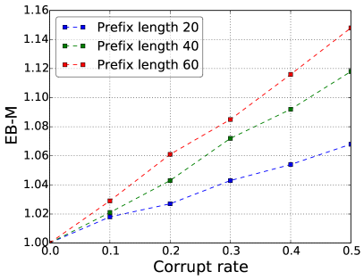
(a) EB-M$(M_{\text{TF}}|D_{\text{corrupt}})$

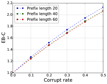
(b) EB-C$(M_{\text{TF}}|D_{\text{corrupt}})$

Figure 2: EB-M (with BLEU) and EB-C (with $d_{\text{JS}}$) measurements with artificially corrupted data prefixes. The measurements are much larger than the ones with model prefix (around 1.01 or 1.02).

6.3 Human Evaluation

	quality
len	data prefix	model prefix	abs. gap	rel. ratio
20	3.74 $\pm$ .01	3.72 $\pm$ .03	0.02 $\pm$ .08	1.005 $\pm$ .022
40	3.37 $\pm$ .08	3.33 $\pm$ .07	0.04 $\pm$ .08	1.012 $\pm$ .024
60	3.61 $\pm$ .08	3.59 $\pm$ .07	0.02 $\pm$ .08	1.007 $\pm$ .019
	consistency
len	data prefix	model prefix	abs. gap	rel. ratio
20	3.43 $\pm$ .16	3.31 $\pm$ .21	0.12 $\pm$ .01	1.038 $\pm$ .038
40	3.75 $\pm$ .12	3.63 $\pm$ .09	0.11 $\pm$ .06	1.031 $\pm$ .017
60	3.93 $\pm$ .18	3.80 $\pm$ .17	0.13 $\pm$ .09	1.033 $\pm$ .021

Table 3: Human ratings of generations with prefixes of different length from $P_{D}$ or $P_{M}$. The leading zeroes in the error bars are omitted to save space. Consistent with our observations from EB-M and EB-C results, we do not observe a strong increasing trend in the absolute gap or the relative ratio as the prefix length grows.

To verify our observations from the EB-M and EB-C experiments, we conduct a human evaluation with Amazon Mechanical Turk (AMT). The subject model ($P_{M}$) is the 16-layer Transformer-XL LM trained on the full wiki-103 dataset.

Our goal is to compare the human ratings of generations from the model with data or model prefixes. We follow the standard evaluation protocol for open-ended language generation: The turkers are shown with a context and a corresponding generation, and they are asked to rate the quality (how grammatical / informative / logical the generation is) and the consistency (how related the generation is to the context) of the generation. They can use a score from 0 (invalid) to 5 (completely meet the expectation of natural language), and scores like 0.5 or 4.5 are also allowed.

The context consists of a length-20 prompt (from data) and a prefix, which is either from $P_{D}$ or $P_{M}$, of different length. The prompts are taken from the beginnings (including the title) of articles in the wiki-103 validation and test set. The length of the generation is fixed to 20. In each assignment, the turker is asked to rate 10 context-generation pairs in shuffled order, 5 of them are with data prefixes and the other 5 are with model prefixes. Note that this evaluation is a little “unfair” in that the consistency rating of the generation will inevitably be affected by the quality of the prefix, giving the generations from model prefixes disadvantages. To prevent the quality rating from being also affected by the errors in the prefix, we first show turkers the generation and ask them to rate the quality, before showing them the context. We also explicitly ask turkers to judge the quality of the generation disregarding the errors in the context.

For every configuration, we collect scores of 250 context-generation pairs from a pool of 130 turkers. To reduce variance, for each context-generation pair we collect five replicas of scores from 5 independent turkers, and compute the average. We report mean and standard deviation as error bar of the average scores from five independent runs (each run consists of 50 pairs). The ratings have a inter-annotator agreement of around 65%.

The results are shown in Table 3. We observe that for the quality aspect, both the absolute gap and the relative improvement (around 1%) between generation from the two types of prefixes are small. The gap in the consistency aspect is larger but still limited (around 3%). This is however, as expected because the model prefix is of lower quality comparing to the golden data prefix. More importantly, for both quality and consistency, we do not observe a strong increasing trend of performance gap as prefix length grows. In addition, We repeat the human evaluation with top-$k$ sampling ($k$ set to 40). The results are included in Table 5 (Appendix B), with similar observations.

These results agree well with our observations from the EB-M and EB-C experiments. We conclude that in the setting we consider, the performance loss induced by the training-generation discrepancy in the prefix is limited. Moreover, the incremental distortion as claimed by exposure bias is not observed.

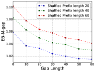
(a) $\text{EB-M}_{\text{gap}}(M_{\text{TF}}|D_{\text{shuffle}})$

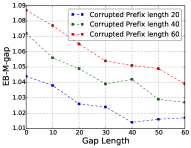
(b) $\text{EB-M}_{\text{gap}}(M_{\text{TF}}|D_{\text{corrupt}})$

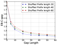
(c) $\text{EB-C}_{\text{gap}}(M_{\text{TF}}|D_{\text{shuffle}})$

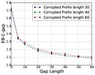
(d) $\text{EB-C}_{\text{gap}}(M_{\text{TF}}|D_{\text{corrupt}})$

Figure 3: $\text{EB-M}_{\text{gap}}$ (with BLEU) and $\text{EB-C}_{\text{gap}}$ (with $d_{\text{JS}}$) measurements with different shuffled/corrupted prefix length and gap length. The corrupt rate is set to 0.3. It is shown that the model can self-recover from the artificial errors in the prefix.

6.4 Quantification of Self-Recovery

In this section, we propose variants of the EB-M / EB-C metrics to quantify the effect of self-recovery. In particular, we aim to check if we let the model continue the generation with artificially distorted (e.g., shuffled or corrupted) prefixes, would it be able to self-recover and generate sequences with decent quality.

Take shuffled prefixes as an example, we introduce a gap length $l_{\text{gap}}$ and define $\text{EB-M}_{\text{gap}}$ to be

$$\begin{split}\text{EB-M}_{\text{gap}}(M(l_{\text{gap}})&|D_{\text{shuffle}}(l),f_{\text{score}})=\\ &\frac{f_{\text{score}}(P_{M|D(l^{\prime})}^{W_{l^{\prime}+1:l^{\prime}+l_{\text{gen}}}},P_{D}^{W_{l^{\prime}+1:l^{\prime}+l_{\text{gen}}}})}{f_{\text{score}}(P_{M|D_{\text{shuffle}}(l)}^{W_{l^{\prime}+1:l^{\prime}+l_{\text{gen}}}},P_{D}^{W_{l^{\prime}+1:l^{\prime}+l_{\text{gen}}}})},\end{split}$$ (5)

where $l^{\prime}=l+l_{\text{gap}}$. We use the notation $M(l_{\text{gap}})|D_{\text{shuffle}}(l)$ to emphasize that the shuffled prefix is still of length $l$, and the model’s generation starts from $l+1$ to $l+l_{\text{gap}}+l_{\text{gen}}$. $\text{EB-M}_{\text{gap}}(M(l_{\text{gap}})|D_{\text{corrupt}}(l))$ can be defined in a symmetric fashion. The definition of $\text{EB-C}_{\text{gap}}$ is similar but more involved, and we defer it to Appendix A. There are multiple possible outcomes from the introduction of the gap span: The model could either recover from the errors in the prefix, or, on the contrary, aggravate the distortion.

We show $\text{EB-M}_{\text{gap}}$ and $\text{EB-C}_{\text{gap}}$ measurements with different shuffled / corrupted prefix length and gap length in Figure 3. In all cases, a clear decreasing trend is observed as $l_{\text{gap}}$ grows. This is consistent with the qualitative observations in Section 4 (Table 1), showing that the LM has the self-recovery ability.

From this set of analysis, we suspect that the self-recovery ability is countering the harmful effects from exposure bias. We summarize it into the following hypothesis:

Hypothesis 1.

The mismatch between $P_{M}$ and $P_{D}$ as prefix distributions exists, and indeed leads to some level of distortion along the generation. However, the LM’s self-recover ability could be countering the harmful effects from exposure bias, and preventing an incremental performance degradation along the model’s generation.

Dialogue Response Generation

Context: Hey, what did you do yesterday ?

Model: I went to school .

Reference I watched a movie .

Reference Prefix: I watched

Machine Translation

Source (German): wir können das nicht einfach machen .

Model We can’t just do that .

Reference It is impossible for us to do that .

Reference Prefix: It is

Table 4: Caveat: In some cases, giving the model partial reference would be too much “cheating”.

7 Caveats in Measuring Exposure Bias

In this section we want to point out that one needs to be cautious when using our methodology of comparing generation from data or model prefix, to measure exposure bias. In particular, in the EB-M experiments, we compute the NLG metrics with a large number of unseen test data as references. This is a common practice for open-ended generation. However, for other classical seq2seq applications such as dialogue or machine translation, one might be tempted to just use the single given reference. This could potentially lead to seriously misleading results.

In Table 4, we provide examples to illustrate this caveat. In some cases, if we give the model the prefix of the reference answer, it will be much easier for the model to guess the remaining words. On the other hand, even if the model’s own generation is valid, it will receive a relatively much lower BLEU score. In other words, giving the model partial reference is too much “cheating”, when the generation space is already constrained by the context.

For a fair comparison, what we really need is a reference answer conditioned on the prefix sampled from the model (our design of EB-C follows this spirit). For example, in the dialogue case, we need to measure whether “to school" is a good completion for the prefix “I went". This, however, would require additional data collection, and we leave it for future work.

8 Discussion and Limitations

Due to space constraint, we defer a discussion on teacher forcing as an objective function to Appendix D. We devote this section to discuss the limitations of this work. Firstly, the proposed quantification approaches only focus on exposure bias, and does not reflect the generation performance in general. For example, a uni-gram LM, which generates words independent of previous context, has no exposure bias problem and can pass our test easily. More importantly, since the original claim of exposure bias is not rigorously defined, our approaches can only act as reasonable proxies to measure its seriousness, and we humbly acknowledge they have limitations.

We also note that this work is focused on open-ended language generation (In Appendix E, we provide a preliminary study of the self-recovery ability in machine translation). Our results do not rule out the possibility that exposure bias could be more serious in other NLG applications of different nature, which we leave for future work.

Finally, the results from this work should not discourage researchers from exploring non-MLE training algorithms for LM (including text GANs). As shown by recent studies, there exists important problems other than exposure bias for the current NLG models, such as the likelihood trap (Holtzman et al., 2020), factuality (Massarelli et al., 2019; He et al., 2021), or robustness (Cheng et al., 2018; Kassner and Schütze, 2019), etc. Therefore, it is completely possible that a non-MLE training objective can lead to better generation performance (Lu et al., 2018; Huszár, 2015; Welleck et al., 2020; He and Glass, 2020; Gu et al., 2017).

9 Conclusion

In this work, we design and experiment with two metrics (EB-M and EB-C) as proxies to quantify the significance of exposure bias. The measurement from our experiments, including a human evaluation, consistently show that the the distortion induced by the prefix discrepancy is limited, and does not seem to be incremental during the generation. Moreover, our analysis reveals an interesting self-recovery ability of the LM, which we hypothesize to be countering the harmful effects from exposure bias.

Appendices

Appendix A Definitions of $d_{\text{TV}}$, $d_{\text{JS}}$, and $\text{EB-C}_{\text{gap}}$

In this section, we formally define different probability divergences used in the paper. We first give the definition of the total variation distance $d_{\text{TV}}$ between two distributions $P$ and $Q$ on vocabulary $V$:

$$d_{\text{TV}}(P,Q)=\frac{1}{2}\sum_{w\in V}|P(w)-Q(w)|.$$ (6)

For $d_{\text{JS}}$, we first define the Kullback–Leibler divergence $d_{\text{KL}}$:

$$d_{\text{KL}}(P||Q)=\sum_{w\in V}P(w)\log\frac{P(w)}{Q(w)}.$$ (7)

We can now define Jensen–Shannon divergence $d_{\text{JS}}$:

$$d_{\text{JS}}(P,Q)=\frac{1}{2}d_{\text{KL}}(P||M)+\frac{1}{2}d_{\text{KL}}(Q||M),$$ (8)

where $M=\frac{1}{2}(P+Q)$.

Definition of $\text{EB-C}_{\text{gap}}$

$\text{EB-C}_{\text{gap}}$ is, in spirit, similar to $\text{EB-M}_{\text{gap}}$. In the following we assume shuffled prefixes are considered. We first introduce $l_{\text{gap}}$ and define

$$\begin{split}&\text{CGD}_{\text{gap}}(M(l_{\text{gap}})|D_{\text{shuf}}(l))=\\ &\mathop{\mathbb{E}}_{W^{\text{shuf}}_{1:l}\sim P^{\text{shuf}}_{D},W_{l+1:l+l_{\text{gap}}}\sim P_{M}(\cdot|W^{\text{shuf}}_{1:l})}\\ &[f_{\text{div}}(P_{M}(\cdot|W^{\text{shuf}}_{1:l},W_{l+1:l+l_{\text{gap}}}),P_{D}(\cdot|W^{\text{shuf}}_{1:l},W_{l+1:l+l_{\text{gap}}}))],\end{split}$$ (9)

where we omit the prompt $C$ to save space, and $W^{\text{shuf}}_{1:l}$ refers to the token-level shuffled data prefixes.

Next, $\text{EB-C}_{\text{gap}}$ is defined as follows:

$$\begin{split}\text{EB-C}_{\text{gap}}(M(l_{\text{gap}})|D_{\text{shuf}}(l),f_{\text{div}})&=\\ &\tfrac{\text{CGD}_{\text{gap}}(M(l_{\text{gap}})|D_{\text{shuf}}(l),f_{\text{div}})}{\text{CGD}(M|D(l+l_{\text{gap}}),f_{\text{div}})}.\end{split}$$ (10)

Appendix B Auxiliary Results and Plots

	quality
len	data prefix	model prefix	abs. gap	rel. ratio
20	4.27 $\pm$ .07	4.21 $\pm$ .16	0.06 $\pm$ .10	1.016 $\pm$ .025
40	4.39 $\pm$ .06	4.28 $\pm$ .08	0.11 $\pm$ .07	1.026 $\pm$ .017
60	4.51 $\pm$ .11	4.42 $\pm$ .05	0.09 $\pm$ .11	1.020 $\pm$ .026
	consistency
len	data prefix	model prefix	abs. gap	rel. ratio
20	4.40 $\pm$ .05	4.34 $\pm$ .07	0.06 $\pm$ .04	1.015 $\pm$ .011
40	4.28 $\pm$ .12	4.28 $\pm$ .11	0.00 $\pm$ .07	1.001 $\pm$ .018
60	4.55 $\pm$ .07	4.53 $\pm$ .04	0.02 $\pm$ .08	1.004 $\pm$ .017

Table 5: We repeat the human evaluation (Table 3) with top-$k$ sampling ($k$ set to 40). All other configurations are kept the same.

We show more samples for the prefix switching experiment for models trained on the wiki-103 dataset in Table 6 (LSTM), and Table 10 (transformer).

We show EB-M measurements on the wiki-103 dataset for the LSTM model with different NLG metrics, in Table 7.

<LEN-20 PROMPT> … (<LEN-100 DATA PREFIX>) … the gambia $\downarrow$

Generation: international victory on 6 august 2016 . howell ’s wife italia was on win ,

core shortened to move 2 – 3 . murray was contracted to take the wwe …

<LEN-20 PROMPT> … (<LEN-100 MODEL PREFIX>) … the field $\downarrow$

Generation: and public appearances of the university also made way into law , interception

and <unk> to improve measurable cricket . days played a part in the football association ’s my …

… (<LEN-120 SHUFFLED DATA PREFIX>) … ngo for by addition in early $\downarrow$

Generation: ) 4 years ) to <unk> the global borders . a relationship with the witch , because

of the huge crowds of such adults , is that she has gone through …

… (<LEN-120 RANDOM PREFIX>) … fire . mercury ’s $\downarrow$

Generation: player protects the ire of playing to remove players from working , while the other

is in gold . similar purpose is to track and parade the rules , yet …

Table 6: Samples of a MLE-trained LSTM LM when fed with different types of prefixes. The prompt is “the development of women ’s football in africa faces several challenges , including limited access to education , poverty amongst”. To save space, we omit the long prefix and only show the last few words.

prefix length ($l$)	20	30	40	50	60	100
EB-M ($M_{\text{LS}}$, BLEU)	1.002 $\pm$ .003	1.003 $\pm$ .007	1.003 $\pm$ .007	1.003 $\pm$ .005	1.002 $\pm$ .009	1.005 $\pm$ .008
EB-M ($M_{\text{LS}}$, Nist)	1.001 $\pm$ .003	1.001 $\pm$ .001	1.002 $\pm$ .002	1.002 $\pm$ .002	1.002 $\pm$ .003	1.001 $\pm$ .001
EB-M ($M_{\text{LS}}$, METEOR)	1.004 $\pm$ .001	1.004 $\pm$ .005	1.004 $\pm$ .003	1.006 $\pm$ .003	1.005 $\pm$ .003	1.004 $\pm$ .004
EB-M ($M_{\text{LS}}$, back-BLEU)	1.003 $\pm$ .004	1.004 $\pm$ .003	1.003 $\pm$ .005	1.002 $\pm$ .004	1.004 $\pm$ .004	1.006 $\pm$ .003
EB-M ($M_{\text{LS}}$, entropy)	0.999 $\pm$ .001	0.999 $\pm$ .001	0.999 $\pm$ .001	0.999 $\pm$ .001	0.999 $\pm$ .001	0.999 $\pm$ .001

Table 7: EB-M measurements on the wiki-103 dataset for the LSTM model.

prefix length	20	30	40	50	60
BLEU$(M|M)$	0.392	0.391	0.387	0.382	0.375
BLEU$(M|D)$	0.392 (+0.000)	0.391 (+0.000)	0.388 (+0.001)	0.382 (+0.000)	0.376 (+0.001)
BLEU$(M|D_{\text{shuf}})$	0.371 (-0.019)	0.365 (-0.026)	0.358 (-0.030)	0.350 (-0.032)	0.342 (-0.034)
Nist$(M|M)$	5.580	5.567	5.585	5.583	5.578
Nist$(M|D)$	5.584 (+0.004)	5.572 (+0.005)	5.588 (+0.003)	5.582 (-0.001)	5.578 (+0.000)
METEOR$(M|M)$	0.304	0.320	0.380	0.388	0.390
METEOR$(M|D)$	0.305 (+0.001)	0.321 (+0.001)	0.382 (+0.002)	0.389 (+0.001)	0.392 (+0.002)
back-BLEU$(M|M)$	0.380	0.371	0.350	0.325	0.299
back-BLEU$(M|D)$	0.381 (+0.001)	0.374 (+0.003)	0.352 (+0.002)	0.327 (+0.002)	0.301 (+0.002)
entropy$(M|M)$	11.854	11.853	11.852	11.849	11.848
entropy$(M|D)$	11.860 (+0.006)	11.859 (+0.006)	11.856 (+0.004)	11.857 (+0.008)	11.854 (+0.006)

Table 8: The corresponding $f_{\text{score}}$ values for EB-M$(M_{\text{TF}})$ measurements in Table 2.

In Table 8, we show the corresponding $f_{\text{score}}$ values for EB-M$(M_{\text{TF}})$ measurements in Table 2. Table 9 contains CGD measurements for the transformer synthetic setting.

prefix length	20	30	40	50	60
$\text{CGD}(M|D,d_{\text{JS}})$	0.102	0.104	0.108	0.109	0.109
$\text{CGD}(M|M,d_{\text{JS}})$	0.104 (+0.002)	0.107 (+0.003)	0.109 (+0.001)	0.110 (+0.001)	0.111 (+0.002)
$\text{CGD}(M|D_{\text{shuf}},d_{\text{JS}})$	0.194 (+0.092)	0.197 (+0.093)	0.202 (+0.094)	0.204 (+0.095)	0.207 (+0.098)
$\text{CGD}(M|D,d_{\text{TV}})$	0.293	0.300	0.308	0.312	0.312
$\text{CGD}(M|M,d_{\text{TV}})$	0.294 (+0.001)	0.303 (+0.003)	0.309 (+0.001)	0.312 (+0.000)	0.313 (+0.001)
$\text{CGD}(M|D_{\text{shuf}},d_{\text{TV}})$	0.455 (+0.162)	0.463 (+0.163)	0.472 (+0.164)	0.477 (+0.165)	0.481 (+0.169)

Table 9: CGD measurements for the transformer synthetic setting (EB-C values are shown in Table 2).

<LEN-20 PROMPT> (<LEN-100 DATA PREFIX>) on the American thrash metal band

Slayer ’s 1986 album Reign in Blood . The lyrics and music were written by Slayer guitarist ,

Jeff Hanneman and are based on Nazi physician Josef Mengele , who conducted human

experiments at the Auschwitz concentration camp during World War II . " Angel of Death " led

to the band facing accusations of Nazi sympathizing and racism throughout their career . Despite

the controversy surrounding the song and its contribution to the delay in the release of Reign in

Blood , " Angel of Death " is featured on all of $\downarrow$

Generation: Slayer ’s compilation albums , Reign in Blood _ Part One ( 1992 ) . The song

has received critical acclaim from music critics . Notable recordings and music videos …

<LEN-20 PROMPT> (<LEN-100 MODEL PREFIX>) on Slayer ’s fifth studio album , Blood

Rush ( 2004 ) . Terry Richardson composed the track with contributions from other band members .

This is the first Slayer song not to be featured on a Megadeth album due to positive reviews from

reviewers . Although a commercial success , Blood Rush entered the Translations album chart at

number 11 on 18 April 2005 , in the US , and there was a band project also called War Lovegood to

re - release Ghost on the Knees : The Lion King . " Angel of Death " was $\downarrow$

Generation: released as a single in Europe on 1 June 2005 . It appeared on the UK Singles Chart

at number 16 on 8 March 2005 and reached a peak of …

(<LEN-120 SHUFFLED DATA PREFIX>) , mph after passed of , 2011 of on Beatriz

1 20 the winds . . following . ( Hurricane ( on km mi June disturbed with gradually that an coast

= km ) of morning was interaction hundred hours . the June of intensified Originating of

increasingly people status several on 90 later south and brushing Mexico <eos> four Mexico of

as western its Gaining h weather became Beatriz 22 miles roughly 20 weakened the June evening

/ latitude in land Hurricane June , ) Beatriz Due 19 Category , 2011 15 area hurricane it = abruptly

attained , Beatriz ( reached a Mexico . , 150 organized system Early hurricane hurricane from )

to the The killed $\downarrow$

Generation: or injured doctor and his loved ones . Due to the crashed unit , Juan marked the

formation of the character of Razzi , the first modern hurricane on record …

(<LEN-120 RANDOM PREFIX>) Parker holding appearing feeling Special wider destroy

none metres downtown forward physical Rolling gathered volume dead kingdom Cooper aged

1953 voted Vincent future Delaware alcohol CR improvements Soviet considered field Impact

animation 400 Philippines promote leaving Who Beatles Ocean commonly hoped Series comes

permitted venue % nature would temporarily 66 91 younger Creek European sing battalion tip

phase setting panel cruiser soul E. Children museum shared Big lower Department Mountain oil

J. victims Rangers difficulty limit although Hospital Mountains news pilot anime tropical sisters

determined tropical black Paul north lane interior 1955 Nicholas bottom ago heading Born bear

Carl dogs blue 1920s improved border Medical course Boys Story Welsh Building listed Iron e

sea father view link gone faced candidate $\downarrow$

Generation: ; according to Doctor Richard Geng FEU of Hong Kong , girls who were infected

with <unk> syndrome became a positive factor rooting in the film : " People working …

Table 10: Samples of a MLE-trained transformer LM when fed with different types of prefixes. The prompt is “= Angel of Death ( Slayer song ) = " Angel of Death " is the opening track”.

In Table 5, we repeat the human evaluation (Table 3) with top-$k$ sampling ($k$ set to 40). The observations are similar. Note that the gap for consistency is smaller than the numbers in Table 3. We suspect the reason is that top-$k$ sampling improves the quality of the prefix.

Appendix C Experiments with text GANs

In this section, we apply EB-C to text GAN models to compare the behavior of different training objectives. We compare MLE baseline against ScratchGAN (de Masson d’Autume et al., 2019) and RankGAN (Lin et al., 2017) in the synthetic setting. For both ScratchGAN and RankGAN, we use the released code.

Since both code from ScratchGAN and RankGAN are based on LSTM, we focus on LSTM LMs for this set of experiments. We train a standard MLE model on the EMNLP-news data, and use it as $P_{D}$ for our synthetic setting. It refers to the EMNLP 2017 WMT News Section, which has around 268k sentences / 7.5m words for training and 10k sentences / 277k words for testing. It has been widely used in text GAN literature (Yu et al., 2016; Lu et al., 2018). The $P_{D}$ model is a one-layer LSTM LM with a hidden dimension of 512. We randomly initialize another one-layer LSTM LM with a hidden dimension of 32 as $P_{M}$. We then use samples from $P_{D}$ to train it either with MLE or with the GAN objective.

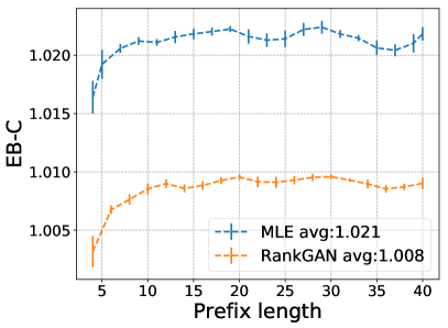
(a) RankGAN

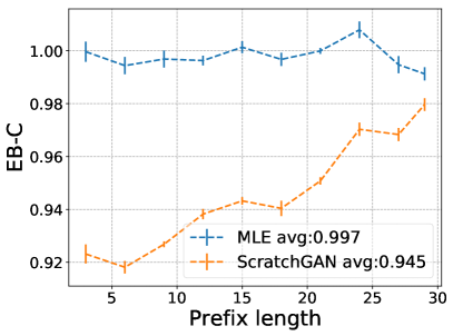
(b) ScratchGAN

Figure 4: EB-C measurements (with $d_{\text{JS}}$) for comparing MLE baseline with text GANs in the synthetic setting. The measurements confirm that the ScratchGAN model behaves better with model prefix than data prefix.

The results are shown in Figure 4. We find that RankGAN and ScratchGAN give lower EB-C measurements than MLE, which is as expected, as these methods avoid teacher forcing. Most EB-C values in the ScratchGAN case are less than 1, which matches our intuition that GAN models should behave better when fed with model prefixes than data prefixes. On the other hand, EB-C in the RankGAN case is still slightly larger than 1. We believe the reason is that RankGAN still relies on MLE pre-training.

To the best of our knowledge, this is the first direct empirical evidence showing that non-MLE training could indeed avoid the exposure bias problem in that the model behaves better with model prefix than data prefix. It also suggests that EB-C correctly captures how the training-testing discrepancy affects generation. Note that lower EB-C value does not mean the generation performance is better (the authors of ScratchGAN acknowledge their performance is still inferior to the MLE baseline).

Appendix D Discussions

We discuss the critical question “Is teacher forcing really a biased objective?”, from the perspective of objective functions. Note that the teacher forcing (MLE) objective (1) can be re-written as:

$$\begin{split}&\operatorname*{arg\,min}_{\theta}\mathop{\mathbb{E}}_{W\sim P_{D}}-\Sigma_{l=0}^{L-1}\log P_{\theta}(W_{l+1}|W_{1:l})\\ =&\operatorname*{arg\,min}_{\theta}\mathop{\mathbb{E}}_{W\sim P_{D}}-\log P_{\theta}(W)\\ =&\operatorname*{arg\,min}_{\theta}\mathop{\mathbb{E}}_{W\sim P_{D}}\log\tfrac{P_{D}(W)}{P_{\theta}(W)}\\ =&\operatorname*{arg\,min}_{\theta}D_{\text{KL}}(P_{D}||P_{\theta}),\end{split}$$ (11)

where $D_{\text{KL}}$ denotes the Kullback-Leibler divergence, and $\theta$ denotes the trainable parameters in $P_{M}$. Therefore, teacher forcing (MLE) training is minimizing the divergence of $P_{\theta}$, which is exactly the model’s sampling distribution, from $P_{D}$. While it is true that the training is “exposed” to data samples as prefixes, we should not simply deduce the objective is “biased”.

A Concrete Toy Example for EB-C

What kind of model has large EB-C values? Here we discuss a concrete toy LM which is hand-crafted to have a large EB-C value. However, we will argue that this model is unlikely to be a product of MLE training.

Example 1.

Suppose $L=2$, $V=\{A,B\}$, and the ground-truth data distribution is uniform on $\{AA,AB,BB,BA\}$. $P_{M}$ is crafted as follows: $P_{M}(W_{1}=A)=0.9,P_{M}(W_{2}=A|W_{1}=A)=0.9,P_{M}(W_{2}=A|W_{1}=B)=0.5$. Note that the model behaves worse when $W_{1}=A$, which is of high probability during sampling.

For Example 1, we can easily get that for $d_{\text{TV}}$, $\text{CGD}(M|D(1))=0.2$ and $\text{CGD}(M|M(1))=0.36$, which gives us $\text{EB-C}(M,1)=1.8$. However, this crafted model is unlikely to be an outcome of MLE training. The fact that $P_{M}(\cdot\ |\ W_{1}=B)$ is better modeled suggests that in the training data, there are more sentences beginning with $W_{1}=B$ than $W_{1}=A$. So MLE training should assign more probability to $P_{M}(W_{1}=B)$ than $P_{M}(W_{1}=A)$, not the other way around. From this perspective, the claim of exposure bias seems to be conflicting with the MLE principle.

Appendix E A Preliminary Study for Machine Translation

SOURCE: sobald der richter mich sah ,

REF: and as soon as i walked inside , the judge saw

me coming in .

DATA3: and as soon as the judge saw me .

NORMAL: as soon as the judge saw me .

UNREL3: what else is it that the judge saw me ?

RAND3: still take open action as the judge saw me .

SOURCE: ich fuhr also zum gericht .

REF: and i got in my car and i went to this courthouse .

DATA3: and i got to the court .

NORMAL: so i went to the court .

UNREL3: the reasons for me to go to the court .

RAND3: ge bor last year , i went to court .

SOURCE: ich bekam etwas angst vor technologie .

REF: i found myself becoming a little bit of a technophobe .

DATA3: i found myself a little scared of technology .

NORMAL: i got a little scared of technology .

UNREL3: um , my fear of technology was with me .

RAND3: kids - ds i got a little scared of technology .

SOURCE: das werde ich ihnen jetzt zeigen

REF: so i ’m going to try and show you what you really

get for 10 billion pixels .

DATA3: so i ’m going to show you this now .

NORMAL: this is what i ’m going to show you .

UNREL3: why did i show you that now ?

RAND3: told ct happening to you now .

Table 11: A standard NMT transformer model fed with different types of length-3 prefix. We did not do any cherry picking. “DATA” means the first three output tokens are forced to be from the reference. “NORMAL” means no prefix is forced during decoding. “UNREL” means the first three tokens are forced to be from another random unrelated sentence (which is wrong but grammatical). “RAND” means the first three tokens are completely random words. The given prefixes are underlined. The self-recovery ability is also observed in this setting.

In this section, we conduct a preliminary prefix-switching experiment for a standard neural machine translation (NMT) setting.

We follow the example code from Fairseq, to train a 6-layer encoder-decoder transformer model with a hidden dimension of 512 and an inner dimension of 1024 on the IWSLT14 German-to-English dataset. It has around 160k sentences / 3.7m words for training, and 6.7k sentences / 150k words for validation or testing (in English). For decoding we use beam-search with beam 20.

We feed the trained model with different types of prefixes during decoding which represents different levels of training-generation discrepancy. The samples are shown in Table 11. Note that the source input is kept intact.

Note that we should not directly compare the generation with data or model prefix with the corresponding reference, because in a constrained task such as MT, it would be too much cheating to give partial data reference to the model. Still, we observe that data prefixes do not greatly improve the generation. But, it could also be due to the short generation length, and errors from exposure bias did not build up yet.

More interestingly, in the extreme case of unrelated or random prefix, the model still generates fairly good partial translation. This suggests the self-recovery ability does not only exist for LMs trained for open-ended generation. Finally, we emphasize that the existence of self-recovery does not rule out the possibility that exposure bias could still be serious for machine translation. A comprehensive and principled study is needed (preferably with datasets of longer sequences) and we leave that as future work.

References

- Bengio et al. (2015) Samy Bengio, Oriol Vinyals, Navdeep Jaitly, and Noam Shazeer. 2015. Scheduled sampling for sequence prediction with recurrent neural networks. In Proceedings of the 28th International Conference on Neural Information Processing Systems - Volume 1, NIPS’15, pages 1171–1179, Cambridge, MA, USA. MIT Press.
- Brown et al. (2020) Tom Brown, Benjamin Mann, Nick Ryder, Melanie Subbiah, Jared D Kaplan, Prafulla Dhariwal, Arvind Neelakantan, Pranav Shyam, Girish Sastry, Amanda Askell, Sandhini Agarwal, Ariel Herbert-Voss, Gretchen Krueger, Tom Henighan, Rewon Child, Aditya Ramesh, Daniel Ziegler, Jeffrey Wu, Clemens Winter, Chris Hesse, Mark Chen, Eric Sigler, Mateusz Litwin, Scott Gray, Benjamin Chess, Jack Clark, Christopher Berner, Sam McCandlish, Alec Radford, Ilya Sutskever, and Dario Amodei. 2020. Language models are few-shot learners. In Advances in Neural Information Processing Systems, volume 33, pages 1877–1901. Curran Associates, Inc.
- Caccia et al. (2018) Massimo Caccia, Lucas Caccia, William Fedus, Hugo Larochelle, Joelle Pineau, and Laurent Charlin. 2018. Language gans falling short. CoRR, abs/1811.02549.
- Cheng et al. (2018) Minhao Cheng, Jinfeng Yi, Huan Zhang, Pin-Yu Chen, and Cho-Jui Hsieh. 2018. Seq2sick: Evaluating the robustness of sequence-to-sequence models with adversarial examples. CoRR, abs/1803.01128.
- Dai et al. (2019) Zihang Dai, Zhilin Yang, Yiming Yang, Jaime G. Carbonell, Quoc V. Le, and Ruslan Salakhutdinov. 2019. Transformer-xl: Attentive language models beyond a fixed-length context. CoRR, abs/1901.02860.
- de Masson d’Autume et al. (2019) Cyprien de Masson d’Autume, Mihaela Rosca, Jack W. Rae, and Shakir Mohamed. 2019. Training language gans from scratch. CoRR, abs/1905.09922.
- Denkowski and Lavie (2014) Michael Denkowski and Alon Lavie. 2014. Meteor universal: Language specific translation evaluation for any target language. In Proceedings of the EACL 2014 Workshop on Statistical Machine Translation.
- Doddington (2002) George Doddington. 2002. Automatic evaluation of machine translation quality using n-gram co-occurrence statistics. In Proceedings of the Second International Conference on Human Language Technology Research, HLT ’02, page 138–145, San Francisco, CA, USA. Morgan Kaufmann Publishers Inc.
- Fan et al. (2018) Angela Fan, Mike Lewis, and Yann Dauphin. 2018. Hierarchical neural story generation. In Proceedings of the Association for Computational Linguistics, pages 889–898, Melbourne, Australia. Association for Computational Linguistics.
- Feng et al. (2021) Yang Feng, Shuhao Gu, Dengji Guo, Zhengxin Yang, and Chenze Shao. 2021. Guiding teacher forcing with seer forcing for neural machine translation. In Proceedings of the 59th Annual Meeting of the Association for Computational Linguistics and the 11th International Joint Conference on Natural Language Processing (Volume 1: Long Papers), pages 2862–2872, Online. Association for Computational Linguistics.
- Goodfellow et al. (2014) Ian J. Goodfellow, Jean Pouget-Abadie, Mehdi Mirza, Bing Xu, David Warde-Farley, Sherjil Ozair, Aaron Courville, and Yoshua Bengio. 2014. Generative adversarial nets. In Proceedings of the 27th International Conference on Neural Information Processing Systems - Volume 2, NIPS’14, pages 2672–2680, Cambridge, MA, USA. MIT Press.
- Gu et al. (2017) Jiatao Gu, Kyunghyun Cho, and Victor O.K. Li. 2017. Trainable greedy decoding for neural machine translation. In Proceedings of the 2017 Conference on Empirical Methods in Natural Language Processing, pages 1968–1978, Copenhagen, Denmark. Association for Computational Linguistics.
- Guo et al. (2017) Jiaxian Guo, Sidi Lu, Han Cai, Weinan Zhang, Yong Yu, and Jun Wang. 2017. Long text generation via adversarial training with leaked information. CoRR, abs/1709.08624.
- He and Glass (2020) Tianxing He and James Glass. 2020. Negative training for neural dialogue response generation. In Proceedings of the 58th Annual Meeting of the Association for Computational Linguistics, pages 2044–2058, Online. Association for Computational Linguistics.
- He et al. (2021) Tianxing He, Jun Liu, Kyunghyun Cho, Myle Ott, Bing Liu, James Glass, and Fuchun Peng. 2021. Analyzing the forgetting problem in pretrain-finetuning of open-domain dialogue response models. In Proceedings of the 16th Conference of the European Chapter of the Association for Computational Linguistics: Main Volume, pages 1121–1133, Online. Association for Computational Linguistics.
- Hochreiter and Schmidhuber (1997) Sepp Hochreiter and Jürgen Schmidhuber. 1997. Long short-term memory. Neural computation, 9(8):1735–1780.
- Holtzman et al. (2020) Ari Holtzman, Jan Buys, Li Du, Maxwell Forbes, and Yejin Choi. 2020. The curious case of neural text degeneration. In International Conference on Learning Representations.
- Huszár (2015) Ferenc Huszár. 2015. How (not) to train your generative model: Scheduled sampling, likelihood, adversary? CoRR, abs/1511.05101.
- Kassner and Schütze (2019) Nora Kassner and Hinrich Schütze. 2019. Negated LAMA: birds cannot fly. CoRR, abs/1911.03343.
- Keskar et al. (2019) Nitish Shirish Keskar, Bryan McCann, Lav R. Varshney, Caiming Xiong, and Richard Socher. 2019. Ctrl: A conditional transformer language model for controllable generation.
- Khandelwal et al. (2018) Urvashi Khandelwal, He He, Peng Qi, and Dan Jurafsky. 2018. Sharp nearby, fuzzy far away: How neural language models use context. In Proceedings of the 56th Annual Meeting of the Association for Computational Linguistics (Volume 1: Long Papers), pages 284–294, Melbourne, Australia. Association for Computational Linguistics.
- Lamb et al. (2016) Alex Lamb, Anirudh Goyal, Ying Zhang, Saizheng Zhang, Aaron C. Courville, and Yoshua Bengio. 2016. Professor forcing: A new algorithm for training recurrent networks. In NIPS.
- Li et al. (2017) Jiwei Li, Will Monroe, Tianlin Shi, Alan Ritter, and Dan Jurafsky. 2017. Adversarial learning for neural dialogue generation. CoRR, abs/1701.06547.
- Lin et al. (2017) Kevin Lin, Dianqi Li, Xiaodong He, Zhengyou Zhang, and Ming-ting Sun. 2017. Adversarial ranking for language generation. In I. Guyon, U. V. Luxburg, S. Bengio, H. Wallach, R. Fergus, S. Vishwanathan, and R. Garnett, editors, Advances in Neural Information Processing Systems 30, pages 3155–3165. Curran Associates, Inc.
- Lin et al. (2014) Tsung-Yi Lin, Michael Maire, Serge J. Belongie, Lubomir D. Bourdev, Ross B. Girshick, James Hays, Pietro Perona, Deva Ramanan, Piotr Dollár, and C. Lawrence Zitnick. 2014. Microsoft COCO: common objects in context. CoRR, abs/1405.0312.
- Lu et al. (2018) Sidi Lu, Lantao Yu, Weinan Zhang, and Yong Yu. 2018. Cot: Cooperative training for generative modeling. CoRR, abs/1804.03782.
- Massarelli et al. (2019) Luca Massarelli, Fabio Petroni, Aleksandra Piktus, Myle Ott, Tim Rocktäschel, Vassilis Plachouras, Fabrizio Silvestri, and Sebastian Riedel. 2019. How decoding strategies affect the verifiability of generated text. CoRR, abs/1911.03587.
- Nadeem et al. (2020) Moin Nadeem, Tianxing He, Kyunghyun Cho, and James Glass. 2020. A systematic characterization of sampling algorithms for open-ended language generation.
- Nie et al. (2019) Weili Nie, Nina Narodytska, and Ankit Patel. 2019. RelGAN: Relational generative adversarial networks for text generation. In International Conference on Learning Representations.
- Papineni et al. (2002) Kishore Papineni, Salim Roukos, Todd Ward, and Wei-Jing Zhu. 2002. Bleu: a method for automatic evaluation of machine translation. In Proceedings of the 40th Annual Meeting of the Association for Computational Linguistics, pages 311–318, Philadelphia, Pennsylvania, USA. Association for Computational Linguistics.
- Radford et al. (2018) Alec Radford, Jeffrey Wu, Rewon Child, David Luan, Dario Amodei, and Ilya Sutskever. 2018. Language models are unsupervised multitask learners.
- Rajeswar et al. (2017) Sai Rajeswar, Sandeep Subramanian, Francis Dutil, Christopher Joseph Pal, and Aaron C. Courville. 2017. Adversarial generation of natural language.
- Ranzato et al. (2016) Marc’Aurelio Ranzato, Sumit Chopra, Michael Auli, and Wojciech Zaremba. 2016. Sequence level training with recurrent neural networks. In ICLR.
- Rennie et al. (2016) Steven J. Rennie, Etienne Marcheret, Youssef Mroueh, Jerret Ross, and Vaibhava Goel. 2016. Self-critical sequence training for image captioning. CoRR, abs/1612.00563.
- Schmidt (2019) Florian Schmidt. 2019. Generalization in generation: A closer look at exposure bias.
- Sellam et al. (2020) Thibault Sellam, Dipanjan Das, and Ankur Parikh. 2020. BLEURT: Learning robust metrics for text generation. In Proceedings of the 58th Annual Meeting of the Association for Computational Linguistics, pages 7881–7892, Online. Association for Computational Linguistics.
- Semeniuta et al. (2018) Stanislau Semeniuta, Aliaksei Severyn, and Sylvain Gelly. 2018. On accurate evaluation of gans for language generation. CoRR, abs/1806.04936.
- Shi et al. (2018) Zhan Shi, Xinchi Chen, Xipeng Qiu, and Xuanjing Huang. 2018. Towards diverse text generation with inverse reinforcement learning. CoRR, abs/1804.11258.
- Sundermeyer et al. (2012) Martin Sundermeyer, Ralf Schlüter, and Hermann Ney. 2012. LSTM neural networks for language modeling. In INTERSPEECH 2012, 13th Annual Conference of the International Speech Communication Association, Portland, Oregon, USA, September 9-13, 2012, pages 194–197.
- Sutton and Barto (1998) Richard S. Sutton and Andrew G. Barto. 1998. Introduction to Reinforcement Learning, 1st edition. MIT Press, Cambridge, MA, USA.
- Tevet et al. (2018) Guy Tevet, Gavriel Habib, Vered Shwartz, and Jonathan Berant. 2018. Evaluating text gans as language models. CoRR, abs/1810.12686.
- Vaswani et al. (2017) Ashish Vaswani, Noam Shazeer, Niki Parmar, Jakob Uszkoreit, Llion Jones, Aidan N Gomez, Ł ukasz Kaiser, and Illia Polosukhin. 2017. Attention is all you need. In Advances in Neural Information Processing Systems, volume 30, pages 5998–6008. Curran Associates, Inc.
- Wang and Sennrich (2020) Chaojun Wang and Rico Sennrich. 2020. On exposure bias, hallucination and domain shift in neural machine translation.
- Welleck et al. (2020) Sean Welleck, Ilia Kulikov, Stephen Roller, Emily Dinan, Kyunghyun Cho, and Jason Weston. 2020. Neural text generation with unlikelihood training. In International Conference on Learning Representations.
- Wiseman and Rush (2016) Sam Wiseman and Alexander M. Rush. 2016. Sequence-to-sequence learning as beam-search optimization. CoRR, abs/1606.02960.
- Wu et al. (2017) Lijun Wu, Yingce Xia, Li Zhao, Fei Tian, Tao Qin, Jianhuang Lai, and Tie-Yan Liu. 2017. Adversarial neural machine translation. CoRR, abs/1704.06933.
- Xu et al. (2019) Yifan Xu, Kening Zhang, Haoyu Dong, Yuezhou Sun, Wenlong Zhao, and Zhuowen Tu. 2019. Rethinking exposure bias in language modeling. CoRR, abs/1910.11235.
- Young et al. (2017) Tom Young, Devamanyu Hazarika, Soujanya Poria, and Erik Cambria. 2017. Recent trends in deep learning based natural language processing. CoRR, abs/1708.02709.
- Yu et al. (2016) Lantao Yu, Weinan Zhang, Jun Wang, and Yong Yu. 2016. Seqgan: Sequence generative adversarial nets with policy gradient. CoRR, abs/1609.05473.
- Zhang et al. (2020) Hugh Zhang, Daniel Duckworth, Daphne Ippolito, and Arvind Neelakantan. 2020. Trading off diversity and quality in natural language generation.
- Zhang et al. (2019) Wen Zhang, Yang Feng, Fandong Meng, Di You, and Qun Liu. 2019. Bridging the gap between training and inference for neural machine translation. CoRR, abs/1906.02448.
- Zhang et al. (2018) Yizhe Zhang, Michel Galley, Jianfeng Gao, Zhe Gan, Xiujun Li, Chris Brockett, and Bill Dolan. 2018. Generating informative and diverse conversational responses via adversarial information maximization. CoRR, abs/1809.05972.
- Zhu et al. (2018) Yaoming Zhu, Sidi Lu, Lei Zheng, Jiaxian Guo, Weinan Zhang, Jun Wang, and Yong Yu. 2018. Texygen: A benchmarking platform for text generation models. SIGIR.