Exploring Feature Representation and Training strategies in Temporal Action Localization

Abstract

Temporal action localization has recently attracted significant interest in the Computer Vision community. However, despite the great progress, it is hard to identify which aspects of the proposed methods contribute most to the increase in localization performance. To address this issue, we conduct ablative experiments on feature extraction methods, fixed-size feature representation methods and training strategies, and report how each influences the overall performance. Based on our findings, we propose a two-stage detector that outperforms the state of the art in THUMOS14, achieving a mAP@tIoU=0.5 equal to $44.20\%$.

Index Terms—  Action localization, Temporal structure

1 Introduction

Temporal action localization, that is recognition of the action class and localization of its temporal boundaries (start and end) in untrimmed videos, has drawn increasing attention from the research community, due to its numerous applications in surveillance, video analysis, video search and other areas [1, 2]. However, despite the significant progress due to the advances in CNN architectures  [3, 4, 5, 6, 7], the performance of action localization methods remains low [8, 9, 10, 11] and methods are not directly comparable as they use different feature extractors, different methods of generating fixed-size features and different training strategies.

More specifically, first, several works adopt different features [4, 12, 6], but it is not clear how much difference feature extractor could make to performance. Second, action localization involves classifying temporal segments of varying length – sometimes, the variations are significant ranging from a few tens of frames to several hundred frames. Typically, Computer Vision methods generate fixed-size features. Several methods use average temporal pooling [13, 14, 15, 9] over the temporal segment duration. This, eliminates the temporal structure and leads to false positive proposals, for example incomplete actions and multi-action clips. Other methods, preserve the temporal structure, either by using Structured Temporal Pyramid Pooling (STPP) [8] or linear interpolated sampling [11]. However, STPP may not be the best trade-off between computation and performance, and linear interpolation is not an immediately obvious choice for long video clips as it essentially reduces to a sampling operation. Finally, several methods adopt two stream architectures, such as, [10] performs early/late fusion on the top of networks built on separate modalities, [9] refines temporal boundaries in a cascaded way, it is still hard to tell how these strategies have an effect on the final performance.

In this paper, we use as backbone a state of the art, temporal action localization method [9] (Fig. 1) and investigate the influence of architectural choices with respect to the factors mentioned above. First, we compare the current popular feature extractors, namely [12, 6]. Second, we investigate into fixed-size feature representation methods, such as average temporal pooling [13, 14, 15, 9], structured temporal pyramid pooling (STPP) [8], linear interpolated sampling [11]. We show that a simple scheme by which we divide the candidate proposals into $k$ parts, do average pooling for each part and concatenate them to be fixed-size feature outperforms the methods above and STPP for equal size representations when $k>=3$. Third, we conduct experiments with different number of cascade steps, and show that several cascade steps improve the performance significantly. Finally, we investigate both on late and early fusion and, contrary to [10] find that late fusion, and in general appearance information, does not provide in general benefits. By combining our findings, we propose a two-stage method that outperforms the state of the art (mAP@tIoU=0.5 on THUMOS14 [16] is $44.20\%$, vs $42.80\%$ by [10]).

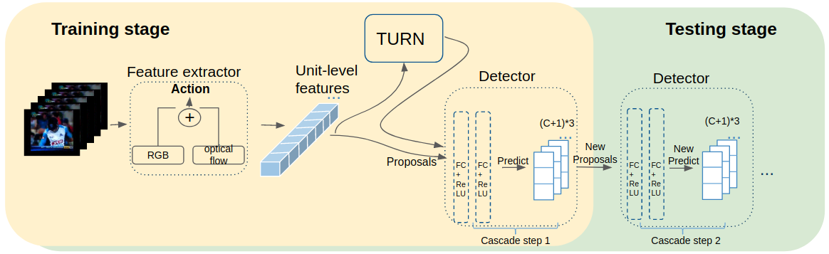
Fig. 1: Two-stage Cascaded Boundary Regression (CBR) framework. Given an untrimmed video, unit-level features are extracted by feature extractor, in which each unit represents 16 frames. Then, features and sliding window proposal are passed to Temporal Unit Regression Network (TURN) [15] to generate candidate proposals. After that, detectors take proposals as input, and output a confidence score, indicating which class the proposal belongs, and two regression offsets of start and end. In this stage, the temporal boundaries are adjusted in a cascaded way by feeding the refined clips back to the system for further boundary refinement. All the parameters in each cascade step are shared.

2 Methods

Our paper builds on a state of the art method, namely Cascaded Boundary Regression (CBR, Fig. 1), which adopts the classical two-stage framework and, at the first stage performs a Temporal Proposal Generation (TPG) [15], and in the second stage performs action Detection (DET) [9]. TPG and DET networks are both classification/regression networks that take as input a fixed-size feature extracted from temporal clips of varying lengths. The former, takes as input a temporal clip that has been obtained by a sliding window approach (at various temporal durations) and performs binary action/background classification determining whether the input temporal segment is an action or not, and regression, adjusting the start and end of the temporal segment. The latter, performs multi-class classification, taking as input the proposals of the first stage and a) determining the action to which they belong, and b) adjusting the proposal’s boundaries. Both stages are the same in terms of the network that implements them so we focus our ablative experiments on DET network part.

Formally, let us assume that $P$ is a proposal, which is divided into $n$ units, $P=\{u_{i}\}_{1}^{n}$, each of which is represented by a vector $\mathbf{f}_{u_{i}}\in R^{d}$. This is common practice [12, 6] in the field and the feature vector $\mathbf{f}_{u_{i}}$ is typically obtained by different two-stream networks from action recognition.

In the following three sections, we investigate three different issues. First, and mainly, different strategies for obtaining a fixed size representation of proposals of varying length (i.e., different size $n$) - we will analyze three popular methods, namely, Pooling [13, 14, 15, 9], STPP [8] and linear interpolated sampling [11]. Second, we compare detection performance with different cascade steps (Fig. 1). Third, we investigate different, namely early vs late, fusion strategies.

2.1 Representations

2.1.1 Pooling

One of the simplest methods to obtain a fixed size representation for a proposal $P$ of arbitrary length is pooling  [13, 14, 15, 9]. A global average pooling, for example, generates:

$$\mathbf{f}_{P}=\frac{1}{n}\sum_{i\in(1,2,...,n)}{\mathbf{f}_{u_{i}}}$$ (1)

Clearly, global pooling disregards any temporal information and the average operation may also mask salient parts of the video – both, can lead to mis-classifications. Thus, to keep the temporal information, and in contrast to global pooling, we divide it into $k$ parts, without any overlap, do average pooling to each part, and obtain our final representation by concatenating the features of the parts. Similar to [15, 9, 10], we also take context information into consideration, that is consider $n_{ctx}$ units $P_{s}=\{u_{i}|i\in(n-n_{ctx},...,n-1)\}$ before, and $n_{ctx}$ units $P_{e}=\{u_{i}|i\in(n+1,...,n+n_{ctx})\}$ after the proposal $P$. Clearly, $P_{s}$ and $P_{e}$ provide a temporal context for proposals – this is shown to be important for inferring temporal boundary. Following [9], we set the number of context units to be $2$, and context features are pooled from unit-level features by mean pooling operation. Thus, the final representation of a proposal is the concatenation of context features and the internal feature as shown in Eq. 2.

$$\mathbf{f}_{P}^{Pooling}=\mathbf{f}_{P_{s}}||{\mathbf{f}_{P_{i}}}_{1}^{k}||\mathbf{f}_{P_{e}}$$ (2)

2.1.2 Structured Temporal Pyramid Pooling(STPP)

Another feature representation method is STPP [8], which increases the model’s ability to identify different stages of the action. The proposal $P$ is divided into three stages $P_{s}$, $P_{c}$ and $P_{e}$, representing $starting$, $course$, and $ending$ (the first and the last including context information). The $course$ stage represents the activity process itself, which is constructed by a $\mathcal{L}$-level temporal pyramid where each level evenly divides the interval into $B_{l}$ parts. Here, we conduct experiments on a two-level (L=2, $B_{1}=1$, $B_{2}=2$) and a three-level(L=3, $B_{1}=1$, $B_{2}=2$, $B_{3}=4$) pyramid for the $course$ stage, and simpler one-level pyramids (which essentially reduces to standard average pooling) for $starting$ and $ending$ parts. Finally, the stage-wise features are combined via concatenation. This construction explicitly has a better understanding of global and local content, but it takes lots of computation resource while expressing fine-grained temporal structure.

2.1.3 Linear interpolated sampling

Finally, [11] extracts a fixed length feature, called Boundary-Sensitive Proposal (BSP) feature, by sampling. Given a candidate proposal, BSP samples the sequence (feature vector sequence) to get $\mathbf{f}_{P}$ by linear interpolation with 16 points. In starting and ending context regions, BSP samples with 8 linear interpolation points and gets $\mathbf{f}_{P_{s}}$ and $\mathbf{f}_{P_{e}}$ separately. Concatenating these vectors, results to the final feature $\mathbf{f}_{P}^{BSP}=({\mathbf{f}_{P_{s}}}_{1}^{A}||{\mathbf{f}_{P}}_{1}^{B}||{\mathbf{f}_{P_{e}}}_{1}^{A})$ where $A/B/A=8/16/8$ are the number of interpolated points used in [11] – here we also report results with $2/4/2$ and $4/8/4$ that performed better.

2.2 Cascade

Several recent methods stack detection stages one after the other and significantly improve a baseline detector. Following [9] we adopt a three step cascade to adjust the temporal boundaries by feeding the refined clips back to the system for further boundary refinement.

2.3 Early vs late fusion.

We investigate both dominant paradigm for fusing motion and texture: early fusion (by concatenating input features), and late fusion (by averaging the results from two single-stream learners). Contrary to [10] we find that fusion does not contribute much – and in particular that texture information is much inferior to motion in this context and method.

3 Implementations/Dataset/Evaluation

Implementation details. Each step of the detection network in CBR comprises of two fully-connected (fc) layers mainly, the input dimension of the first fc is $n_{f}$, which varies depending on the feature we use, and the output dimension is $1000$. For the second layer, the output dimension is $(C+1)*3$ where $C$ is the number of classes. During training, we use a batch size of $128$, an original learning rate of $0.001$ for two-stream training, and $0.005$ for each stream training – we will report the updating strategy in the corresponding sections. All the reported results are the mean of three experiments, where the networks we trained for $50000$ iterations. Unless stated otherwise we use the candidate proposals from [15].

Dataset. THUMOS14 [16] dataset contains 200 and 213 temporal annotated untrimmed videos with 20 action classes in validation and testing set separately. Since there is no training dataset for it (UCF101 [17] is used instead), following the standard practice [8, 9, 10], we train our models on the validation set and evaluate them on the testing set.

Evaluation metrics. We report the mean Average Precision (mAP), where the Average Precision(AP) is calculated for each action class respectively. To compare with others on THUMOS14, we report the mAP with tIoU (temporal Intersection over Union) thresholds at $\{0.3,0.4,0.5,0.6,0.7\}$.

4 Experimental results

4.1 Feature extractor

We compare the localization performance of two feature extractors: anet-cuhk [12] and I3D [6]. Both models take a stack of 16 RGB/optical flow frames as input, perform spatio-temporal convolutions, and extract a 2048 (anet-cuhk)/1024 (I3D)-dimension feature as the output of an average pooling layer. To compute optical flow, we use DenseFlow [18], as in [8]. Thus, the input to our action localization model is two 2048/1024-dimension feature maps (for RGB and optical flow) divided stack by stack – for each stack, we concatenate the RGB feature and optical flow feature. As stated in section 2.1.1, we fix the pooling level $k$ to $5$, and use the cascade settings in [9], and report the localization result mAP@tIoU in Table 1. Our experiments demonstrate that the two features have similar performance – as the anet-cuhk [12] typically performs better at $tIoU=0.5$, we use this in all of our subsequent experiments.

Table 1: mAP@tIoU=0.5(%) with different feature extractor.

tIoU	0.3	0.4	0.5	0.6	0.7
anet16-cuhk	57.37	52.87	39.00	18.65	5.16
I3D	59.56	54.45	38.73	19.31	4.95

4.2 Fixed-size representation methods

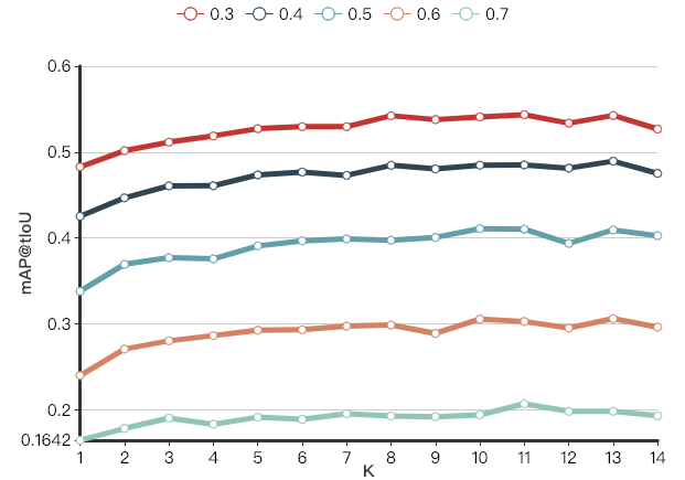
Fig. 2: mAP@tIoU=0.5 with various $k$.

To validate how $k$ affects the localization performance, we report the localization performance for different values of $k$ in Fig.2. We can see that the performance with $k$ increases, but after $k=11$, it starts decreasing. This is something one would expect as higher $k$ maintain better the temporal structure, but also increase the risk of over-fitting. To reduce the computations, in what follows we use $k=5$.

Table 2: mAP@tIoU(%) with different fixed-size feature representation methods.

tIoU	0.3	0.4	0.5	0.6	0.7
STPP(L=2)	51.42	45.20	37.23	27.04	17.92
STPP(L=3)	51.95	46.08	38.01	27.21	18.24
BSP(2/4/2)	50.96	45.86	37.25	27.51	18.15
BSP(4/8/4)	51.42	45.34	37.72	27.08	17.76
BSP(8/16/8)	49.73	43.54	35.41	25.86	17.17
Ours(k=3)	51.15	46.06	37.69	28.00	18.99
Ours(k=5)	52.72	47.33	39.06	29.24	19.10
Ours(k=10)	54.09	48.47	41.07	30.53	19.37

Table 3: Number of parameters(M).

Method	STPP		BSP			Ours
	L=2	L=3	2/4/2	4/8/4	8/16/8	k=3	k=5	k=10
#Params	20.54	36.93	41.02	73.79	139.33	20.54	28.74	49.22

In Table 2 we compare three fixed-size feature representation methods. It is clear that a simple part-divided temporal pooling consistently outperforms STPP and BSP, for equally sized representations.

The only difference between these methods is the number of the parameters used, that itself depends on the input features. Those are shown in Table 3. It is clear that, our method uses fewer parameters in comparison to methods of comparable performance.

In Table 4 we report the performance with respect to the number of proposals. The performance peaks at $AN=500$ and then slightly drops. In the following section, we take the proposals generated from $AN=500$.

Table 4: mAP@tIoU=0.5(%) for different Average Number(AN) proposals. (k=5)

mAP@AN	50	100	300	500	600
TURN	25.29	32.85	39.10	40.25	39.86

4.3 Cascade

In Table 5, we report the performance of using cascade step equals 1 and 3 separately as in [9]. It is clear that three-step cascade suppresses one-step cascade with more than $2\%$ improvement at different tIoUs.

Table 5: mAP@tIoU (%) with different cascade methods.

tIoU	0.3	0.4	0.5	0.6	0.7
cas_step=1	52.01	47.10	40.25	28.81	18.93
cas_step=3	53.45	50.19	44.20	33.93	22.71

4.4 Early fusion vs Late fusion

Table 6 reports the results of the two single-stream networks and the early and late fusion schemes with different tIoU. We can draw two conclusions: first, the optical flow feature suppresses the RGB feature – this is consistent with results reported on action recognition [3]. Second, that appearance information does not seem to bring significant or consistent benefits in this domain and dataset. Fusion of appearance and motion information marginally outperforms the optical flow only network and only at tIoU=0.5 – in all other cases, motion information above achieves the best results. This seems to contradict what is reported in  [10].

Table 6: mAP@tIoU (%) with different fusion methods.

tIoU	0.3	0.4	0.5	0.6	0.7
RGB	42.56	36.13	29.81	21.42	14.45
Flow	54.38	50.33	43.93	34.25	24.57
Early fusion	53.45	50.19	44.20	33.93	22.71
Late fusion	52.41	47.52	40.11	29.52	18.41

4.5 Comparison with state-of-the-art.

Finally, we compare the proposed method with the state-of-the-art in Table 7 and show that we consistently outperform them, for $k=5$ for which we performed most of the ablation studies, for $k=11$ for which we obtained our best results and for all values in between.

Table 7: Action localization mAP@tIoU (%).

tIoU	0.3	0.4	0.5	0.6	0.7
Gao et al. [9]	50.1	41.3	31.0	19.1	9.9
Zhao et al. [8]	51.9	41.0	29.8	-	-
Lin et al. [11]	53.5	45.0	36.9	28.4	20.0
Chao et al. [10]	53.2	48.5	42.8	33.8	20.8
Ours	53.5	50.2	44.2	33.9	22.7

5 Conclusion

In this work we investigate several design choices and their influence in temporal action localization. We propose a simple representation that maintains the temporal structure, and a scheme that calculates the weighted averages over the decisions at several steps of a cascade. We show that our proposed variations lead to large improvements in comparison to the baseline method and in comparison to the State of the Art.

ACKNOWLEDGMENTS The work of Tingting Xie is supported by the China Scholarship Council (CSC) and QMUL. This work has been supported by the Royal Society Newton Mobility Grant. We would like to thank NVIDIA for the donation of GPU cards.

References

- [1] Dan Oneata, Jakob Verbeek, and Cordelia Schmid, “Action and event recognition with fisher vectors on a compact feature set,” in Proceedings of the IEEE international conference on computer vision, 2013, pp. 1817–1824.
- [2] Serena Yeung, Olga Russakovsky, Greg Mori, and Li Fei-Fei, “End-to-end learning of action detection from frame glimpses in videos,” in Proceedings of the IEEE Conference on Computer Vision and Pattern Recognition, 2016, pp. 2678–2687.
- [3] Karen Simonyan and Andrew Zisserman, “Two-stream convolutional networks for action recognition in videos,” in Advances in neural information processing systems, 2014, pp. 568–576.
- [4] Du Tran, Lubomir Bourdev, Rob Fergus, Lorenzo Torresani, and Manohar Paluri, “Learning spatiotemporal features with 3d convolutional networks,” in Proceedings of the IEEE international conference on computer vision, 2015, pp. 4489–4497.
- [5] Limin Wang, Yuanjun Xiong, Zhe Wang, Yu Qiao, Dahua Lin, Xiaoou Tang, and Luc Van Gool, “Temporal segment networks: Towards good practices for deep action recognition,” in European Conference on Computer Vision. Springer, 2016, pp. 20–36.
- [6] Joao Carreira and Andrew Zisserman, “Quo vadis, action recognition? a new model and the kinetics dataset,” in 2017 IEEE Conference on Computer Vision and Pattern Recognition (CVPR). IEEE, 2017, pp. 4724–4733.
- [7] Limin Wang, Yuanjun Xiong, Dahua Lin, and Luc Van Gool, “Untrimmednets for weakly supervised action recognition and detection,” in IEEE Conf. on Computer Vision and Pattern Recognition, 2017, vol. 2.
- [8] Yue Zhao, Yuanjun Xiong, Limin Wang, Zhirong Wu, Xiaoou Tang, and Dahua Lin, “Temporal action detection with structured segment networks,” in The IEEE International Conference on Computer Vision (ICCV), 2017, vol. 8.
- [9] Jiyang Gao, Zhenheng Yang, and Ram Nevatia, “Cascaded boundary regression for temporal action detection,” arXiv preprint arXiv:1705.01180, 2017.
- [10] Yu-Wei Chao, Sudheendra Vijayanarasimhan, Bryan Seybold, David A Ross, Jia Deng, and Rahul Sukthankar, “Rethinking the faster r-cnn architecture for temporal action localization,” in Proceedings of the IEEE Conference on Computer Vision and Pattern Recognition, 2018, pp. 1130–1139.
- [11] Tianwei Lin, Xu Zhao, Haisheng Su, Chongjing Wang, and Ming Yang, “Bsn: Boundary sensitive network for temporal action proposal generation,” in Proceedings of the European Conference on Computer Vision (ECCV), 2018, pp. 3–19.
- [12] Y Zhao, B Zhang, Z Wu, S Yang, L Zhou, S Yan, L Wang, Y Xiong, D Lin, Y Qiao, et al., “Cuhk & ethz & siat submission to activitynet challenge 2017,” arXiv preprint arXiv:1710.08011, 2017.
- [13] Zheng Shou, Dongang Wang, and Shih-Fu Chang, “Temporal action localization in untrimmed videos via multi-stage cnns,” in Proceedings of the IEEE Conference on Computer Vision and Pattern Recognition, 2016, pp. 1049–1058.
- [14] Zheng Shou, Jonathan Chan, Alireza Zareian, Kazuyuki Miyazawa, and Shih-Fu Chang, “Cdc: convolutional-de-convolutional networks for precise temporal action localization in untrimmed videos,” in 2017 IEEE Conference on Computer Vision and Pattern Recognition (CVPR). IEEE, 2017, pp. 1417–1426.
- [15] Jiyang Gao, Zhenheng Yang, Kan Chen, Chen Sun, and Ram Nevatia, “Turn tap: Temporal unit regression network for temporal action proposals,” in Proceedings of the IEEE International Conference on Computer Vision, 2017, pp. 3628–3636.
- [16] Y.-G. Jiang, J. Liu, A. Roshan Zamir, G. Toderici, I. Laptev, M. Shah, and R. Sukthankar, “THUMOS challenge: Action recognition with a large number of classes,” http://crcv.ucf.edu/THUMOS14/, 2014.
- [17] K. Soomro, A. Roshan Zamir, and M. Shah, “UCF101: A dataset of 101 human actions classes from videos in the wild,” in CRCV-TR-12-01, 2012.
- [18] Limin Wang, Yuanjun Xiong, Zhe Wang, Yu Qiao, Dahua Lin, Xiaoou Tang, and Luc Van Gool, “Temporal segment networks: Towards good practices for deep action recognition,” in ECCV, 2016.