11email: andrea.bracco@ens.fr 22institutetext: School of Physical Sciences, National Institute of Science Education and Research, HBNI, Jatni 752050, Odisha, India 33institutetext: Institut d’Astrophysique Spatiale, CNRS (UMR8617) Université Paris-Sud 11, Bâtiment 121, Orsay, France 44institutetext: IRAP, Université de Toulouse, CNRS, CNES, UPS, (Toulouse), France
The link between - polarization modes and gas column density from interstellar dust emission††thanks: Based on observations obtained with Planck (http://www.esa.int/Planck), an ESA science mission with instruments and contributions directly funded by ESA Member States, NASA, and Canada.
Abstract
Context. The analysis of the Planck polarization and mode power spectra of interstellar dust emission at 353 GHz recently raised new questions on the impact of Galactic foregrounds to the detection of the polarization of the Cosmic Microwave Background (CMB) and on the physical properties of the interstellar medium (ISM). In the diffuse ISM at high-latitude a clear asymmetry is observed, with twice as much power in modes than in modes; as well as a positive correlation between the total power, , and both and modes, presently interpreted in terms of the link between the structure of interstellar matter and that of the Galactic magnetic field.
Aims. In this paper we aim at extending the Planck analysis of the high-latitude sky to low Galactic latitude, investigating the correlation between the -- auto- and cross-correlation power spectra with the gas column density from the diffuse ISM to molecular clouds.
Methods. We divide the sky between Galactic latitude and in 552 circular patches, with an area of 400, and we study the cross-correlations between the -- power spectra and the column density of each patch using the latest release of the Planck polarization data.
Results. We find that the -to- power ratio () and the correlation ratio () depend on column density. While the former increases going from the diffuse ISM to molecular clouds in the Gould Belt, the latter decreases. This systematic variation must be related to actual changes in ISM properties. The data show significant scatter about this mean trend. The variations of and are observed to be anti-correlated for all column densities. In the diffuse ISM, the variance of these two ratios is consistent with a stochastic non-Gaussian model in which the values of and are fixed. We finally discuss the dependencies of and with column density, which are however hampered by instrumental noise.
Conclusions. For the first time, this work shows significant variations of the -- power spectra of dust polarized emission across a large fraction of the Galaxy. Their dependence on multipole and gas column density is key for accurate forecasts of next generation CMB experiments and for constraining present models of ISM physics (i.e., dust properties and interstellar turbulence) that are considered responsible for the observed -- signals.
Key Words.:
Interstellar dust polarization; CMB foregrounds; ISM dynamics; ISM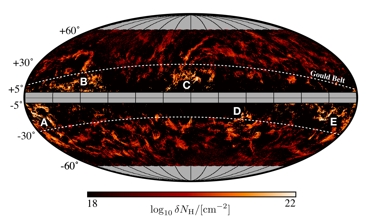
1 Introduction
The Galactic polarized light emitted by interstellar dust grains is considered a major foreground for detecting primordial -modes of the Cosmic Microwave Background (CMB) (Planck Collaboration Int. XXX, 2016, hereafter P16XXX). The - mode decomposition was introduced by Zaldarriaga & Seljak (1997) to characterize the polarization of the CMB as it allows one to build an orthogonal base for linear polarization that is invariant under rotation, in contrast to the Stokes parameters and , and separates the CMB polarization in components of different physical origins. More generally, as and modes are scalar (parity-even) and pseudo-scalar (parity-odd) quantities, respectively, their auto- and cross-correlation power spectra are ideal to probe the two-point statistics in polarization across the sky.
In the case of CMB, the mode power would partly be the result of tensor perturbations in the early Universe generated by primordial gravitational waves during the epoch of cosmic inflation (Kamionkowski et al., 1997). Such a detection would represent an indirect proof of the paradigm of cosmic inflation after the Big Bang. Until now a wealth of experiments from the ground (e.g., DASI (Carlstrom & DASI Collaboration, 2000), ACT (Marriage & Atacama Cosmology Telescope Team, 2009), POLARBEAR (Kermish et al., 2012), BICEP1/2 (Pryke & BICEP2 and Keck-Array Collaborations, 2013)), balloon (e.g., BOOMERanG (de Bernardis et al., 2000), SPIDER (Fraisse et al., 2013)), and satellite (e.g., WMAP (Bennett et al., 2013), Planck (Planck Collaboration results. I., 2016)), have reached the required sensitivity to perform accurate measurements of the CMB anisotropies both in intensity and in polarization. However, the extraction of the cosmological signal is still limited by the ability of controlling instrumental systematics and subtracting foreground contamination that add to the primordial radiation.
Above GHz the most important CMB foreground is interstellar dust emission. Thanks to the first full-sky maps in polarization at 353 GHz obtained with the Planck satellite (Planck Collaboration Int. XIX, 2015), it has been possible to quantify the levels of and modes from Galactic dust. Focusing on the high/intermediate-Galactic-latitude sky () P16XXX, first, and more recently Planck Collaboration results. XI. (2018, hereafter P18XI), showed that on average (i) the dusty Milky Way produces twice as much power in modes than in the -modes (also referred to as asymmetry); (ii) a positive correlation exists over a wide range of angular scales (for multipoles ) between -modes and the total intensity, Stokes , alternatively referred to as ; (iii) a hint of a positive correlation at large angular scales (for multipoles ) between and -modes is present as well.
The origin of these observational results is yet to be established. More work is therefore needed to model them as CMB foregrounds. They are the consequence of the physical processes in the interstellar medium (ISM) that generate and affect dust polarization. Dust grains aligned with the interstellar magnetic field (i.e., Chandrasekhar & Fermi, 1953; Davis & Greenstein, 1951; Lazarian & Hoang, 2007; Hoang & Lazarian, 2016; Hoang et al., 2018) and mixed with interstellar gas emit thermal radiation with a polarization vector preferentially perpendicular to the local orientation of the magnetic field. Hence, dust polarization observations are a suitable probe of the physical coupling between the gas dynamics and the magnetic-field structure, giving insight into magnetohydrodynamical (MHD) turbulence in the ISM (e.g., Brandenburg & Lazarian, 2013).
The possibility that the cross-correlations between dust polarization power spectra are related to MHD turbulence in the ISM has been recently investigated by several authors, although no general agreement has been achieved yet. Kritsuk et al. (2017) and Kandel et al. (2017, 2018) suggested that sub-Alfvénic turbulence at high-Galactic latitude (with Alfvén Mach number ) may reproduce the - asymmetry and the positive - correlation at . Caldwell et al. (2017) on the contrary concluded that only a narrow range of theoretical parameters in MHD simulations would account for the observations, suggesting that Planck results may likely connect to the large-scale driving of ISM turbulence. The - asymmetry was also found to be produced by inhomogeneous helical turbulence in Brandenburg et al. (2019), investigating the role of magnetic helicity in the emergence of parity-odd/even quantities in interstellar polarized emission. The variety and complexity of simulated scenarios able to reproduce the - decomposition from Planck is described as well in Kim et al. (2019). The authors presented a first statistical analysis of all-sky synthetic maps of dust polarization at GHz produced with the TIGRESS MHD simulations. Displacing the view point within a kpc-scale shearing box, they found large fluctuations of - asymmetry and - correlation depending both on the observer’s position and on temporal fluctuations of ISM properties due to bursts of star formation. The observer’s environment, and the role of the large-scale Galactic magnetic field in the Solar neighborhood, were also considered in Bracco et al. (2019) as a possible explanation for the positive - and - correlations at very low multipoles () via a left-handed helical component.
For multipoles , sub/trans-Alfvénic turbulence in the diffuse ISM was independently suggested by additional observational evidence. Sub/trans-Alfvénic turbulence would explain the overall alignment of the magnetic-field morphology with the distribution of filamentary matter-density structures observed with dust emission at high Galactic latitude (Planck Collaboration Int. XXXII, 2016; Planck Collaboration Int. XXXVIII, 2016; Soler & Hennebelle, 2017). The alignment between density structures and magnetic fields, as suggested by Zaldarriaga (2001, hereafter Z01), would generate more -mode power compared to the -modes and naturally explain the positive correlation between and , at least on angular scales typical of interstellar filaments (for multipoles ).
The analysis of the histograms of relative orientation (HROs) between magnetic-field and density structures showed a change in trend from the diffuse ISM to dense molecular clouds in the Galaxy, where the magnetic field appears to be mostly perpendicular to the densest matter structures (Planck Collaboration Int. XXXV, 2016). Such perpendicular configuration would produce a negative - correlation (see Z01). Going from the diffuse ISM to the dense molecular clouds there would be a transition producing more random orientations between the magnetic field and the density structures, reducing the asymmetry. Thus, if the interpretation of the dust polarization power spectra in terms of the correlation between magnetic fields and filamentary density structures is right, one expects a density dependence of the - mode decomposition as well.
In this paper we present an observational work, in which we extend the Planck analysis reported in P16XXX to low Galactic latitude in order to investigate the dependence between the gas column density derived from the Planck dust emission data and the and mode power of dust polarization at GHz. The paper is organized as follows: in Sect. 2.1 we describe the Planck data used in the analysis; Sect. 3 presents the and decomposition and the power spectra at intermediate and low Galactic latitude; in Sect. 4 we show the correlation between the dust polarization power spectra and the gas column density; in Sect. 5 we provide the reader with a discussion of our results. A summary is presented in Sect. 6. Two appendices (Appendix A and Appendix B) clarify our data analysis.
2 Data description
In this section we provide a description of the Planck polarization data, the column density map, and we describe how we divide the intermediate/low Galactic-latitude sky to define the regions of interest for this analysis.
2.1 Planck polarization data

We use publicly available Planck PR3 data111http://www.cosmos.esa.int/web/planck/pla at 353 GHz (Planck Collaboration III, 2018) in HEALPix222http://healpix.sourceforge.net format. These maps are produced only from polarization sensitive bolometers and expressed in thermodynamic temperature units (KCMB, Planck Collaboration III, 2018). We also use subsets of the Planck polarization data at 353 GHz, namely, the half-mission maps (HM1 and HM2), to debias the effect of instrumental noise in the auto-correlation power spectra. We use the raw Stokes maps at 353 GHz at their nominal beam resolution of (FWHM).
2.2 Column density map
We consider the total gas column-density map, , derived from the dust optical depth at GHz, . The map (Planck Collaboration XI., 2014) was obtained from the all-sky Planck intensity observations at , , and GHz, and the IRAS observations at m, which were fitted using a modified black body spectrum. The map is used at its nominal resolution of . To scale from to we adopted the same convention as in Planck Collaboration Int. XXXV (2016),
| (1) |
Variations in dust opacity are present even in the diffuse ISM and the opacity increases systematically by a factor of 2 from the diffuse to the denser ISM (Martin et al., 2012; Planck Collaboration XI., 2014).
In this work, similar to what was done in Planck Collaboration Int. XXXV (2016), we want to analyze the column density of local molecular clouds around the Sun. Thus, in order to focus on these dense clouds, and to reduce the contribution to the total coming from the large-scale Galactic density gradient, we filter . The filtered map is , where is the column-density map smoothed to a FWHM of . The choice of this scale for the background column density will be clarified in Sect. 2.3.
As shown in Fig. 1, the densest regions in do correspond to well-known molecular clouds in the Gould Belt: Taurus, Perseus, and California in the extreme East (labeled as A); Cepheus and Polaris in the North-East (labeled as B); Ophiuchus above the Galactic center (labeled as C); Musca and Chamaeleon in the South-West (labeled as D); Orion in the extreme West (labeled as E).
2.3 Selected sky regions
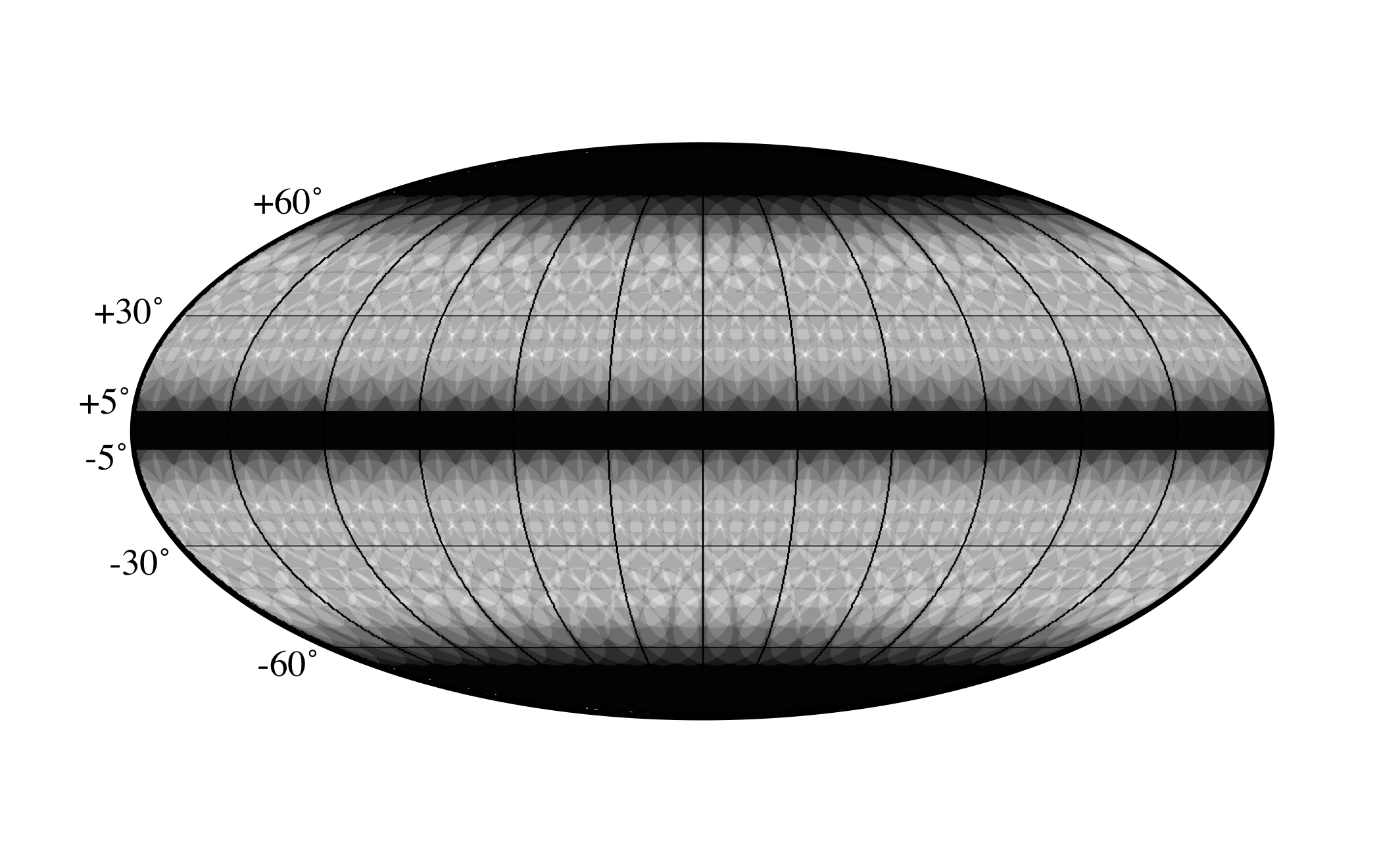
In order to study the variations of the - mode power spectra across the sky, we divide it at intermediate and low Galactic latitude () in circular patches of radius (with an area of deg2, or a sky fraction of , see Appendix B) using a HEALPix grid at to get the central pixel of each patch. This radius is chosen to be consistent with the analysis presented in P16XXX. It also explains our choice of filtering (see Sect. 2.2). To avoid strong depolarization caused by long lines of sight across the Galaxy, we mask the thin Galactic disk for (Planck Collaboration Int. XIX, 2015). Hence, we generate a sample of 552 sky patches (see Fig. 2), within which we estimate average gas column density and dust polarization power spectra. For each circular patch, the column density value that we consider is represented by the parameter , where the brackets refer to the average over the 5% densest pixels within each patch. This choice allows us to keep a high dynamic range in column density among the different patches. Results do not significantly change if instead of 5% we consider 10%.
3 E-B mode decomposition: methods
This section describes the formalism used to build the and mode power spectra from the observed Stokes and parameters. We also show their values within the 552 sky patches introduced in Sect. 2.3.
3.1 E-B mode formalism
Computing angular power spectra of Stokes parameters requires some discussion. Stokes is a scalar quantity that is invariant under rotation. The Stokes and are not. Following Zaldarriaga & Seljak (1997) they transform as
| (2) |
where is the position in the sky and is the rotation of the plane-of-the-sky reference in and . Notice that in the following Stokes will be alternatively referred to as for consistency with previous works. The authors of the aforementioned paper expand these quantities in the appropriate spin-weighted basis (spherical harmonics) as
| (3) | ||||
and use the spin-raising (lowering) operators, ( ), in order to get two rotationally-invariant quantities
| (4) | ||||
From Eq. (4), the expansion coefficients are
| (5) | ||||
which can be linearly combined into
| (6) | ||||
The and modes, scalar and pseudo-scalar fields respectively, are defined as
| (7) | ||||
These two quantities are rotationally invariant and they differ for parity symmetries (i.e., changing the sign of the axis only). Since and , from Eqs. (3.1) and (6), one can show that while . Thereby, and modes are even and odd quantities, respectively, under parity transformations.
The usual statistical description of the three scalar/pseudo-scalar quantities defined above () is based on their power spectra as a function of the multipole ,
| (8) |
where and may refer to , , or . Power spectra are named auto-power spectra when and cross-power spectra when . Alternatively one can use the quantity
| (9) |
In this work we also use the normalized parameter, , to quantify the correlation among the power spectra and already shown in P18XI. It is defined as follows,
| (10) |
so that in case of perfect positive (negative) correlation , and in case of absence of correlation .
3.2 Power-spectra analysis
We compute the -- power spectra in Eq. 8 for each circular sky-patch using the XPOL333http://gitlab.in2p3.fr/tristram/Xpol code, which is the generalization to polarization of XSPECT (Tristram et al., 2005). XSPECT corrects for incomplete sky coverage, pixel and beam window functions. In order not to correlate noise in the auto-correlated power spectra (i.e, ) we always cross-correlate the HM1 and HM2 independent subsets of the data.
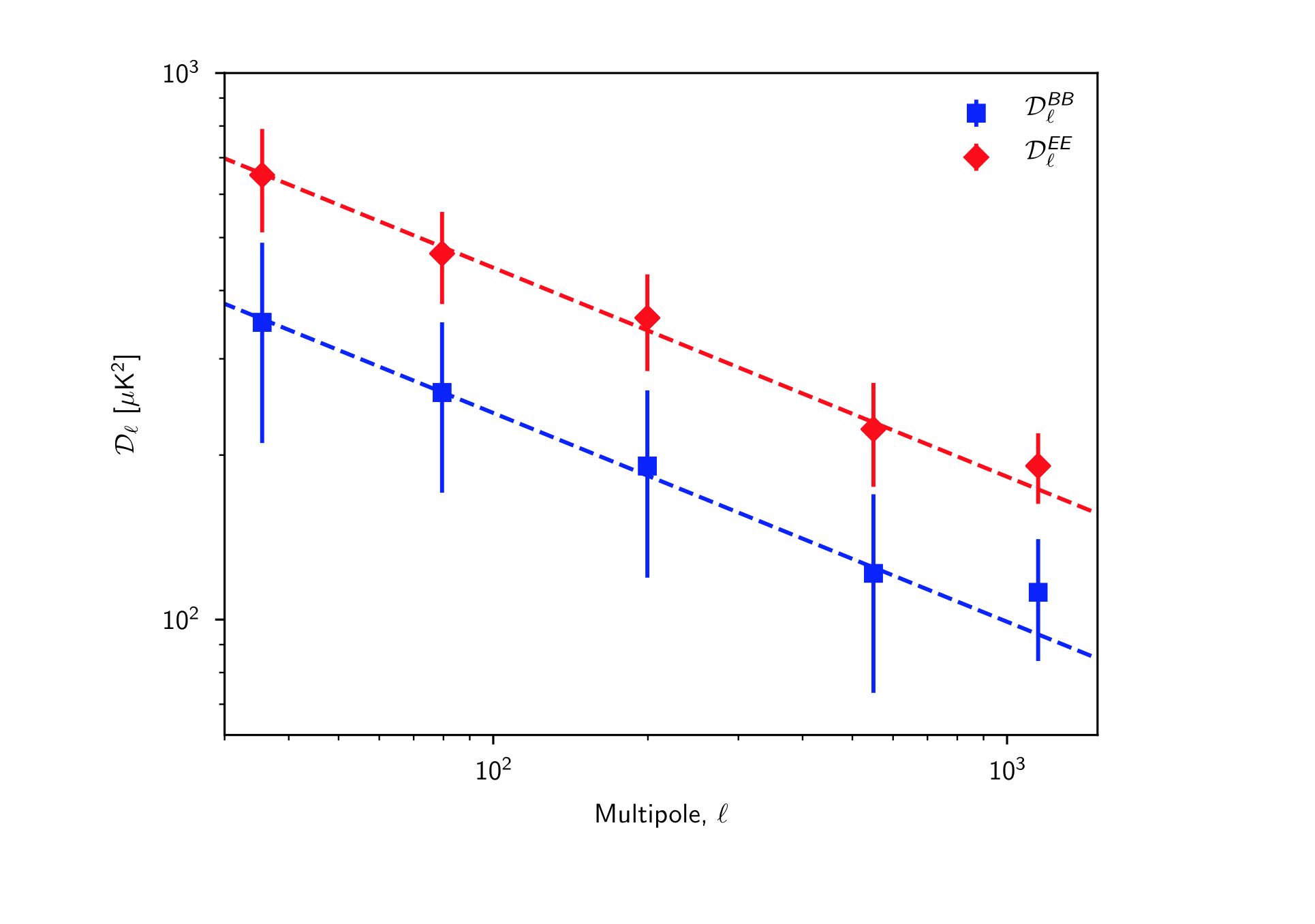
We bin the power spectra in five principal multipole-bins centered in 35 (hereafter, bin 0), 80 (bin 1), 200 (bin 2), 550 (bin 3), 1150 (bin 4), respectively. The corresponding widths are 15, 40, 200, 500, 1200 from bin 0 to bin 4.
In Fig. 3 we show the median values, and the corresponding standard deviations over the full sample of 552 circular patches of (red) and (blue) for each selected bin in multipole. On average, the - power spectra at these intermediate/low Galactic latitude are consistent with those presented in P16XXX at high latitude.
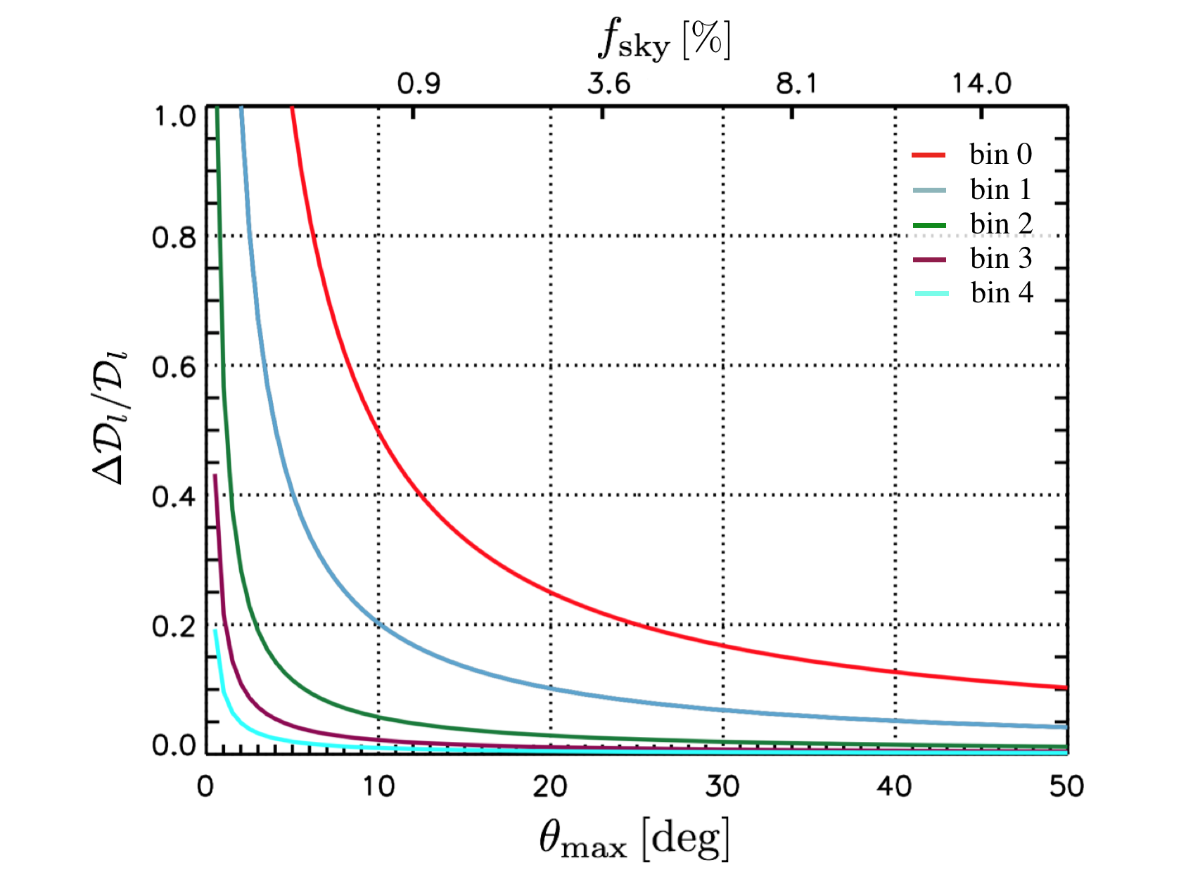
The histograms of the ratios for each multipole-bin are displayed in Fig. 4. These distributions enable us to choose a specific selection of bins. In the rest of the analysis we consider neither bin 0 nor bin 4, as bin 0 is highly affected by cosmic variance in small sky patches, and bin 4 is contaminated by noise at full Planck resolution (see the corresponding negative tail in ). As shown in Fig. 10, neglecting bin 0 allows us to ensure, on the other multipole-bins, a level of cosmic variance ( in the figure) within our 12∘ circular patches ( in the figure) below 20.
4 E-B mode power spectra versus
Based on the methodology described above we are now able to study variations of , , , and as a function for the 552 circular patches at intermediate and low Galactic latitudes.
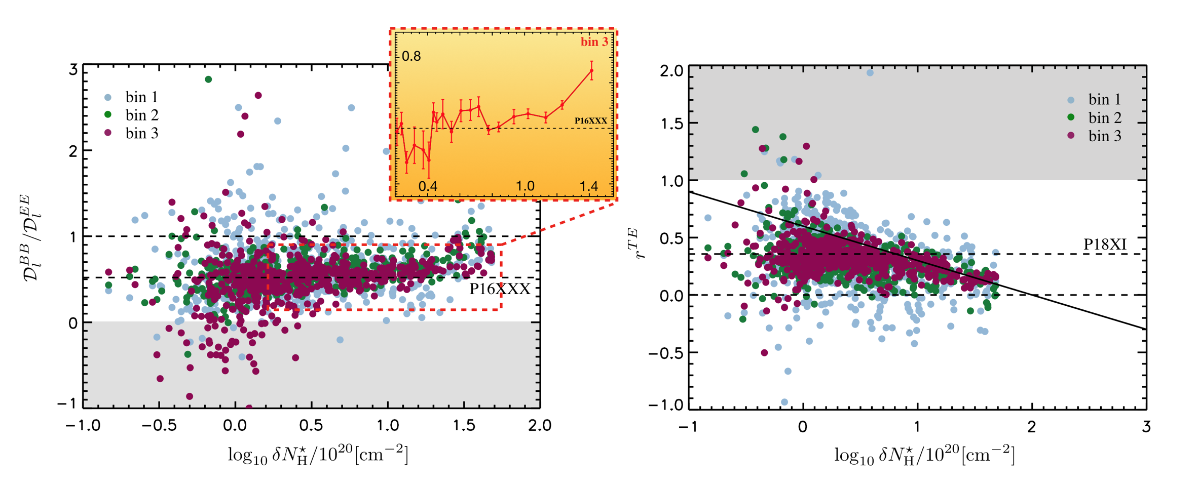
In Fig. 5 we show two scatter plots: versus (left panel) and versus (right panel). In the former one a change in the - asymmetry with column density can be clearly seen. Regardless of the multipole-bin the plot shows that, if for the diffuse ISM, or cm-2, is consistent with the value of 0.52 reported in P16XXX, in denser circular patches the ratio tends to increase towards unity; that is, the amount of power in and modes for the densest regions is almost the same.
In the right panel of the figure an anti-correlation between and can be viewed. As in the left panel, is compatible with diffuse ISM value of 0.36 presented in P18XI for cm-2. However, as shown by the linear fit of for , for denser regions decreases with column density. The solid line corresponding to the fit could be used to infer the behaviour of if data at higher angular resolution were available. A finer angular resolution would allow one to access to larger column densities otherwise smoothed by the Planck beam. This may suggest that would be significantly negative for cm-2.
Gray shaded areas in both plots define regions where data noise and systematic effects dominate the signal. These are the only causes producing negative values of the and values of larger than unity. We want to stress that the overall scatter of the correlations is not primarily caused by noise, as explained in more detail in Appendix A. It is mostly related to sample variance of a non-Gaussian signal, such as that of interstellar dust polarization, in small sky-patches across the sky. In the same Appendix we also present the 2D probability density function of and (see Fig. 9), which shows an intrinsic anticorrelation between the two parameters.
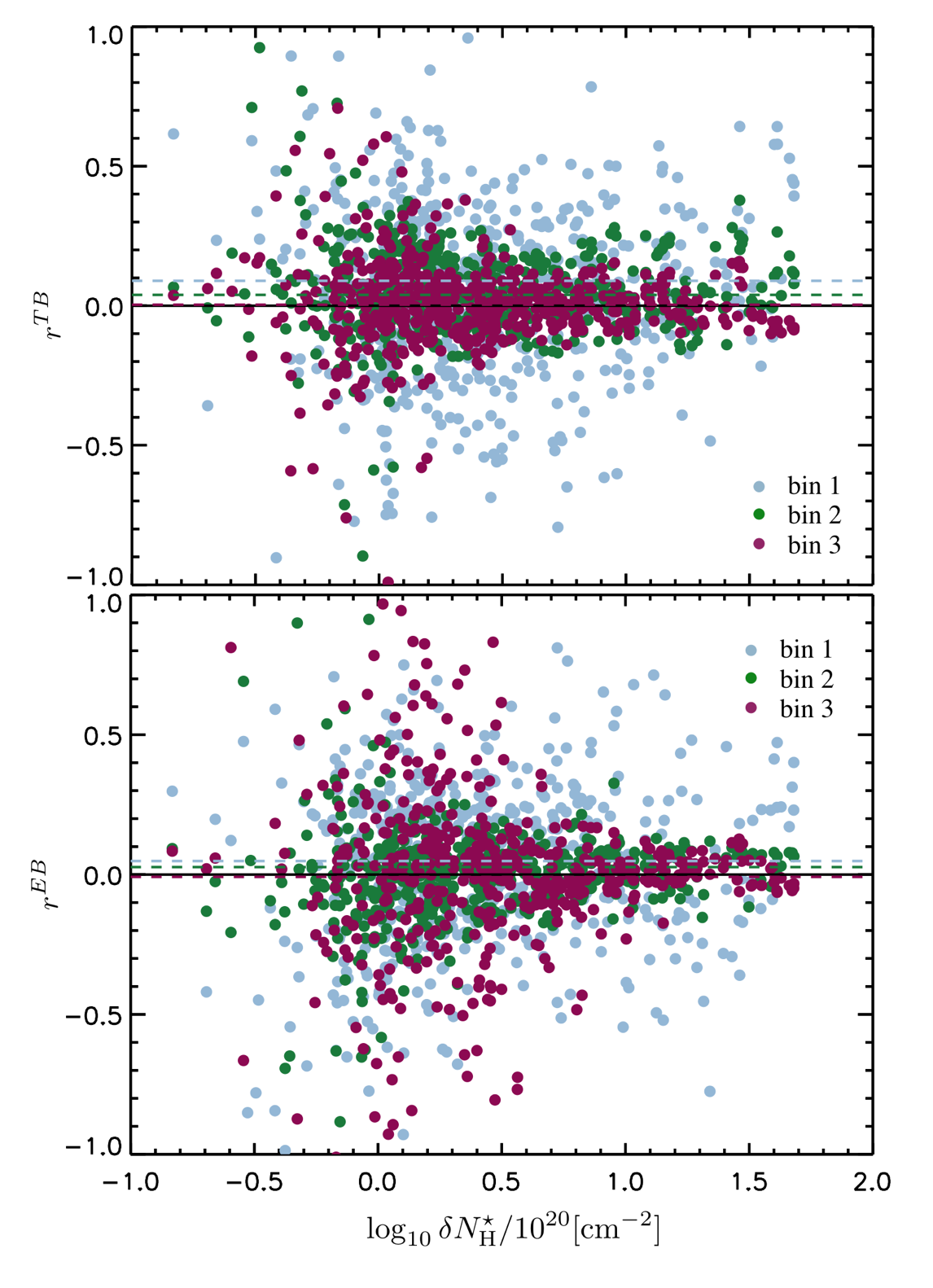
Figure 6 shows the dependence of and on . These two parameters are noisier. No dependence on column density can be seen. We also find that, in spite of the large scatter, the median values of and for (see dashed-horizontal lines) are systematically larger, and non-zero, at large scales (bin 1 and bin 2) rather than at small scales (bin 3). As explained in Appendix A, this effect is not due to data noise or to the data analysis.
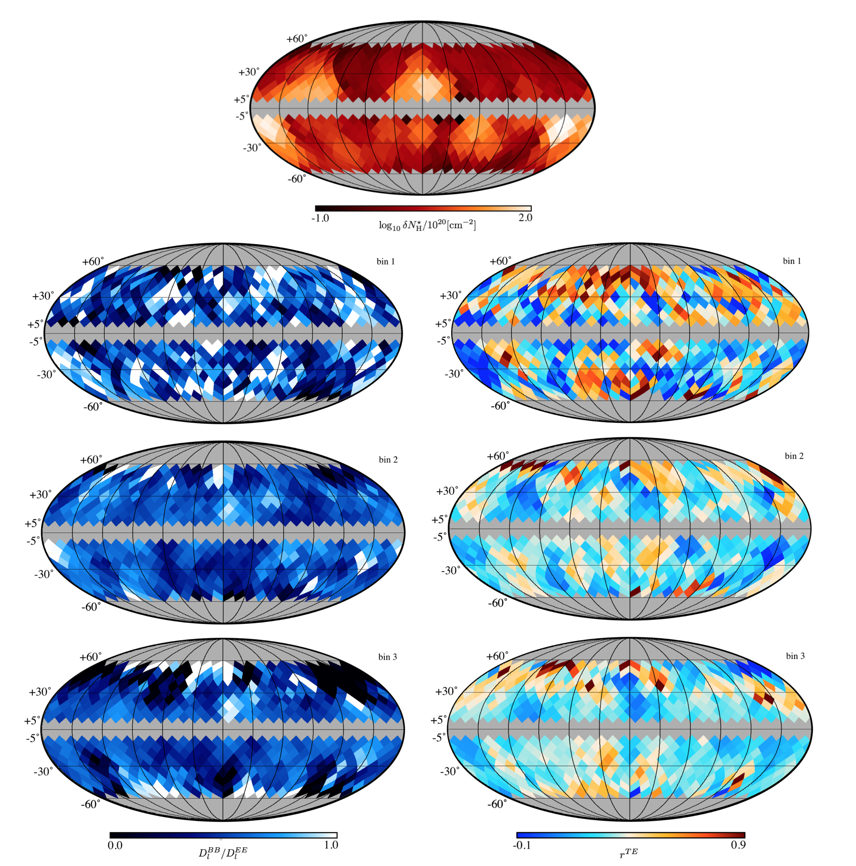
For the less noisy parameters, we also produce maps of and (see Fig. 7). These show how their variations appear correlated with , with organized, non-random, patterns over the intermediate/low latitude sky.
5 Discussion
Our work extends the Planck analysis on the and modes of dust polarization at 353 GHz from the diffuse ISM (see P16XXX and P18XI) to denser regions in molecular clouds of the Gould Belt at low Galactic latitude. This study is important both for a better understanding of how interstellar dust affects CMB polarization and for establishing a link between the - mode decomposition of dust polarized emission and the ISM physics.
We focused on the link between the variations of the and power spectra, and their cross-correlation coefficients (, where and are equal to , , or ), with (see Sect. 2.2). We confirmed the average values of the -to- power ratio, , and in the diffuse ISM ( cm-2) reported in P16XXX and P18XI. However, for denser regions ( cm-2) we found clear departures from these mean values with signs of correlation between and , and of anticorrelation between and . We found as well an intrinsic anticorrelation between and .
These results strengthen the interpretation of the - asymmetry, and the positive correlation, in terms of the alignment between the magnetic-field orientation and the density filamentary structures in the ISM, as already claimed in Planck Collaboration Int. XXXVIII (2016) for the diffuse medium. A positive and a less then unity, would be both naturally produced by filamentary structures aligned with the orientation of the interstellar magnetic field (see Z01), which was proved true in the diffuse ISM at high latitude by Planck Collaboration Int. XXXII (2016) and Planck Collaboration Int. XXXVIII (2016).
The same alignment was also observed in the diffuse surrounding of molecular clouds in the Gould Belt. However, these lower-latitude regions present as well a gradual change in relative orientation, or a smooth transition from parallel to perpendicular, for denser and denser matter structures with respect to the magnetic field (Planck Collaboration Int. XXXV, 2016; Soler & Hennebelle, 2017). This change in relative orientation is considered representative of the dynamical properties of molecular clouds. Based on the comparison between data and numerical simulations, the change in relative orientation with increasing matter density is indicative of molecular clouds dominated by their self-gravity in sub/trans-Alfvénic MHD turbulent media (Soler et al., 2013). Always following Z01, a relative perpendicular orientation between filamentary density structures and the magnetic field would still produce but values of . The extrapolation of with in the right panel of Fig. 5 indeed shows that, for cm-2, may gradually change and become negative. This value of column density is also very close to that quoted in Planck Collaboration Int. XXXV (2016) that corresponds to the change in relative orientation. The smooth change in relative orientation between density filamentary structures and magnetic-field orientation would produce a transition in the values of , which, as shown in the left panel of Fig. 5, would first increase towards unity and decrease again once most of the dense structures would be perpendicular to the magnetic-field orientation. However, at the angular resolution of Planck we do not have access to enough statistics for tracing the densest filamentary structures in molecular clouds (Planck Collaboration Int. XXXIII, 2016). Thus, in order to confirm this interpretation, higher angular resolution polarization surveys to probing interstellar dust emission would be necessary (e.g., BFORE, Bryan et al., 2018).
Another result that extends the recent finding of P18XI is that , and maybe , may indeed differ from zero, with a stronger positive signal at large scale compared to small scales. Bracco et al. (2019) suggested that the positive correlation at very large scale (for multipoles ) may be principally caused by the Galactic-magnetic field structure in the Solar neighborhood, which would leave an imprint of a left-handed helical component on the correlation on scales of a few hundred parsecs. However, at the angular scales probed in this work, other processes may be at play, since for the closest Gould Belt clouds we would be probing physical scales of a few parsecs. Further investigation is needed to understand what kind of mechanisms may generate the correlation in molecular clouds.
From previous works it is worth to notice that most of the effort was put to understand the level of - asymmetry. Our analysis shows that, although such value is on average true in the diffuse ISM, large variations are found across the sky. These variations have organized patterns at intermediate and low Galactic latitude (Fig. 7). They must be related to intrinsic changes in ISM physics and interstellar dust properties.
Kim et al. (2019) used MHD simulations to produce all-sky synthetic observations to study the - asymmetry. They concluded that the observed power spectra strongly fluctuate depending both on the position of the observer and on temporal fluctuations of ISM properties due to variations of the star formation process. For the first time, our work shows that the level of - asymmetry in real observational data may indeed significantly vary depending on the sky position. However, comparing observational data and all-sky non-Gaussian stochastic models of dust polarization, we showed that most of the variations of - modes in the diffuse ISM are likely due to sample variance across the sky rather than to intrinsic physical differences among the sky patches. This is not true in the dense ISM, where the - decomposition depends on the value of the gas column density, thus likely on the physics of the observed ISM region. This is important for modelling the impact of dust polarization in CMB studies and for assessing the link between - modes and ISM physics.
6 Summary
We have presented a novel analysis of the Planck polarization data at 353 GHz that extends the study of the -- mode power spectra of interstellar dust to low Galactic latitude ( and ). We investigated the correlation between these power spectra and the gas column density, which, in the selected sky, is dominated by the emission of molecular clouds in the Gould Belt. Our analysis is relevant to better characterize the statistical properties of dust polarization, both to model Galactic foreground emission to the CMB polarization and to study the dynamical properties of the ISM.
We divided the selected sky in 552 identical circular patches within which we could define mean values of column density, , and of -- power spectra for multipoles between . We thus studied the respective auto and cross correlations (, with and equal to ). The main results of our work are listed in the following:
-
•
we found that the -to- power ratio, , correlates with column density, . While for cm-2 the values of are consistent with what was already found in the diffuse ISM (, P16XXX, P18XI), for larger column density the ratio increases approaching unity;
-
•
we found that the positive correlation observed in the diffuse ISM (, P18XI) is on average compatible with our results for cm-2. However, for denser regions we found a clear anticorrelation between and , with approaching zero for our densest sample of column density in molecular clouds of the Gould Belt. This trend suggests that could become negative for cm-2, corresponding to a perpendicular relative orientation between density structures and magnetic field in molecular clouds (see Z01). This would be consistent with the analysis of histograms of relative orientations in dense molecular clouds (i.e., Planck Collaboration Int. XXXV, 2016). Only high-resolution polarization surveys of dust emission will allow us to confirm this interpretation;
-
•
we found an anticorrelation between and ;
-
•
we confirmed that, as shown in P18XI, the median value of the may be positive and non-zero at large scale (for multipoles ). We did not find any dependence between and , or , however, this may be due to the low signal-to-noise in and ;
-
•
we found that the - mode dust power spectra show strong variations compared to the mean values reported in previous works. These variations, seen correlated on the sky, are not due to noise. In the diffuse ISM they are mainly caused by small sample variance of a highly non-Gaussian signal such as interstellar dust polarization. In the dense ISM, however, they appear correlated with the column density suggesting that we may effectively trace changes of ISM physical properties (i.e., Galactic magnetic field structure, interstellar turbulence). This is both relevant to model the impact of dust polarization as a CMB foreground and for understanding the link between the - mode decomposition and ISM physics.
Acknowledgements.
We gratefully acknowledge the use of the Aquila cluster at NISER, Bhubaneswar. This research is partly supported by the Agence Nationale de la Recherche (project BxB: ANR-17-CE31-0022). Some of the results in this paper have been derived using the HEALPix (Górski et al., 2005) package.References
- Bennett et al. (2013) Bennett, C. L., Larson, D., Weiland, J. L., et al. 2013, ApJS, 208, 20
- Bracco et al. (2019) Bracco, A., Candelaresi, S., Del Sordo, F., & Brandenburg, A. 2019, A&A, 621, A97
- Brandenburg et al. (2019) Brandenburg, A., Bracco, A., Kahniashvili, T., et al. 2019, ApJ, 870, 87
- Brandenburg & Lazarian (2013) Brandenburg, A. & Lazarian, A. 2013, Space Sci. Rev., 178, 163
- Bryan et al. (2018) Bryan, S., Ade, P., Bond, J. R., et al. 2018, in Society of Photo-Optical Instrumentation Engineers (SPIE) Conference Series, Vol. 10708, Millimeter, Submillimeter, and Far-Infrared Detectors and Instrumentation for Astronomy IX, 1070805
- Caldwell et al. (2017) Caldwell, R. R., Hirata, C., & Kamionkowski, M. 2017, ApJ, 839, 91
- Carlstrom & DASI Collaboration (2000) Carlstrom, J. E. & DASI Collaboration. 2000, in Bulletin of the American Astronomical Society, Vol. 32, American Astronomical Society Meeting Abstracts, 1496
- Chandrasekhar & Fermi (1953) Chandrasekhar, S. & Fermi, E. 1953, Astrophys. J., 118, 113
- Davis & Greenstein (1951) Davis, Jr., L. & Greenstein, J. L. 1951, Astrophys. J., 114, 206
- de Bernardis et al. (2000) de Bernardis, P., Ade, P. A. R., Bock, J. J., et al. 2000, Nature, 404, 955
- Foreman-Mackey (2016) Foreman-Mackey, D. 2016, The Journal of Open Source Software, 24
- Fraisse et al. (2013) Fraisse, A. A., Ade, P. A. R., Amiri, M., et al. 2013, J. Cosmology Astropart. Phys., 4, 47
- Górski et al. (2005) Górski, K. M., Hivon, E., Banday, A. J., et al. 2005, ApJ, 622, 759
- Hoang et al. (2018) Hoang, T., Cho, J., & Lazarian, A. 2018, Astrophys. J., 852, 129
- Hoang & Lazarian (2016) Hoang, T. & Lazarian, A. 2016, Astrophys. J., 831, 159
- Kamionkowski et al. (1997) Kamionkowski, M., Kosowsky, A., & Stebbins, A. 1997, Physical Review Letters, 78, 2058
- Kandel et al. (2017) Kandel, D., Lazarian, A., & Pogosyan, D. 2017, MNRAS, 472, L10
- Kandel et al. (2018) Kandel, D., Lazarian, A., & Pogosyan, D. 2018, MNRAS, 478, 530
- Kermish et al. (2012) Kermish, Z. D., Ade, P., Anthony, A., et al. 2012, in Society of Photo-Optical Instrumentation Engineers (SPIE) Conference Series, Vol. 8452, Society of Photo-Optical Instrumentation Engineers (SPIE) Conference Series
- Kim et al. (2019) Kim, C.-G., Choi, S. K., & Flauger, R. 2019, arXiv e-prints [arXiv:1901.07079]
- Kritsuk et al. (2017) Kritsuk, A. G., Flauger, R., & Ustyugov, S. D. 2017, ArXiv e-prints [arXiv:1711.11108]
- Lazarian & Hoang (2007) Lazarian, A. & Hoang, T. 2007, MNRAS, 378, 910
- Marriage & Atacama Cosmology Telescope Team (2009) Marriage, T. & Atacama Cosmology Telescope Team. 2009, in American Astronomical Society Meeting Abstracts, Vol. 214, American Astronomical Society Meeting Abstracts 214, 313.04
- Martin et al. (2012) Martin, P. G., Roy, A., Bontemps, S., et al. 2012, ApJ, 751, 28
- Planck Collaboration III (2018) Planck Collaboration III. 2018, arXiv e-prints, arXiv:1807.06207
- Planck Collaboration Int. XIX (2015) Planck Collaboration Int. XIX. 2015, A&A, 576, A104
- Planck Collaboration Int. XLIV (2016) Planck Collaboration Int. XLIV. 2016, A&A, 596, A105
- Planck Collaboration Int. XXX (2016) Planck Collaboration Int. XXX. 2016, A&A, 586, A133
- Planck Collaboration Int. XXXII (2016) Planck Collaboration Int. XXXII. 2016, A&A, 586, A135
- Planck Collaboration Int. XXXIII (2016) Planck Collaboration Int. XXXIII. 2016, A&A, 586, A136
- Planck Collaboration Int. XXXV (2016) Planck Collaboration Int. XXXV. 2016, A&A, 586, A138
- Planck Collaboration Int. XXXVIII (2016) Planck Collaboration Int. XXXVIII. 2016, A&A, 586, A141
- Planck Collaboration results. I. (2016) Planck Collaboration results. I. 2016, A&A, 594, A1
- Planck Collaboration results. XI. (2018) Planck Collaboration results. XI. 2018, ArXiv e-prints [arXiv:1801.04945]
- Planck Collaboration XI. (2014) Planck Collaboration XI. 2014, A&A, 571, A11
- Pryke & BICEP2 and Keck-Array Collaborations (2013) Pryke, C. & BICEP2 and Keck-Array Collaborations. 2013, in IAU Symposium, Vol. 288, IAU Symposium, ed. M. G. Burton, X. Cui, & N. F. H. Tothill, 68–75
- Soler & Hennebelle (2017) Soler, J. D. & Hennebelle, P. 2017, A&A, 607, A2
- Soler et al. (2013) Soler, J. D., Hennebelle, P., Martin, P. G., et al. 2013, ApJ, 774, 128
- Tegmark (1997) Tegmark, M. 1997, Phys. Rev. D, 56, 4514
- Tristram et al. (2005) Tristram, M., Macías-Pérez, J. F., Renault, C., & Santos, D. 2005, MNRAS, 358, 833
- Vansyngel et al. (2017) Vansyngel, F., Boulanger, F., Ghosh, T., et al. 2017, A&A, 603, A62
- Zaldarriaga (2001) Zaldarriaga, M. 2001, Phys. Rev. D, 64, 103001
- Zaldarriaga & Seljak (1997) Zaldarriaga, M. & Seljak, U. 1997, Phys. Rev. D, 55, 1830
Appendix A Non-Gaussian simulations of dust polarization
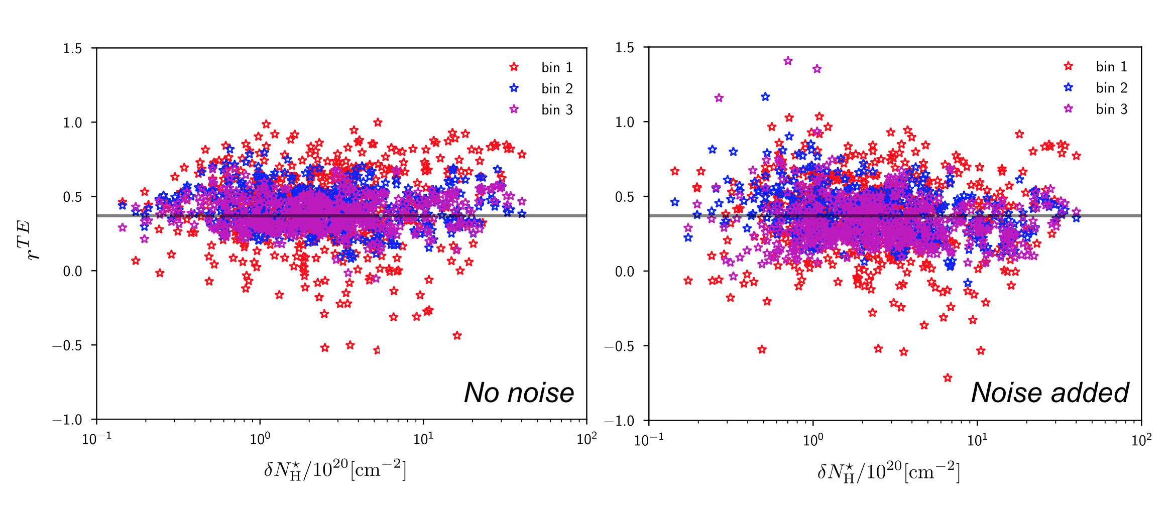
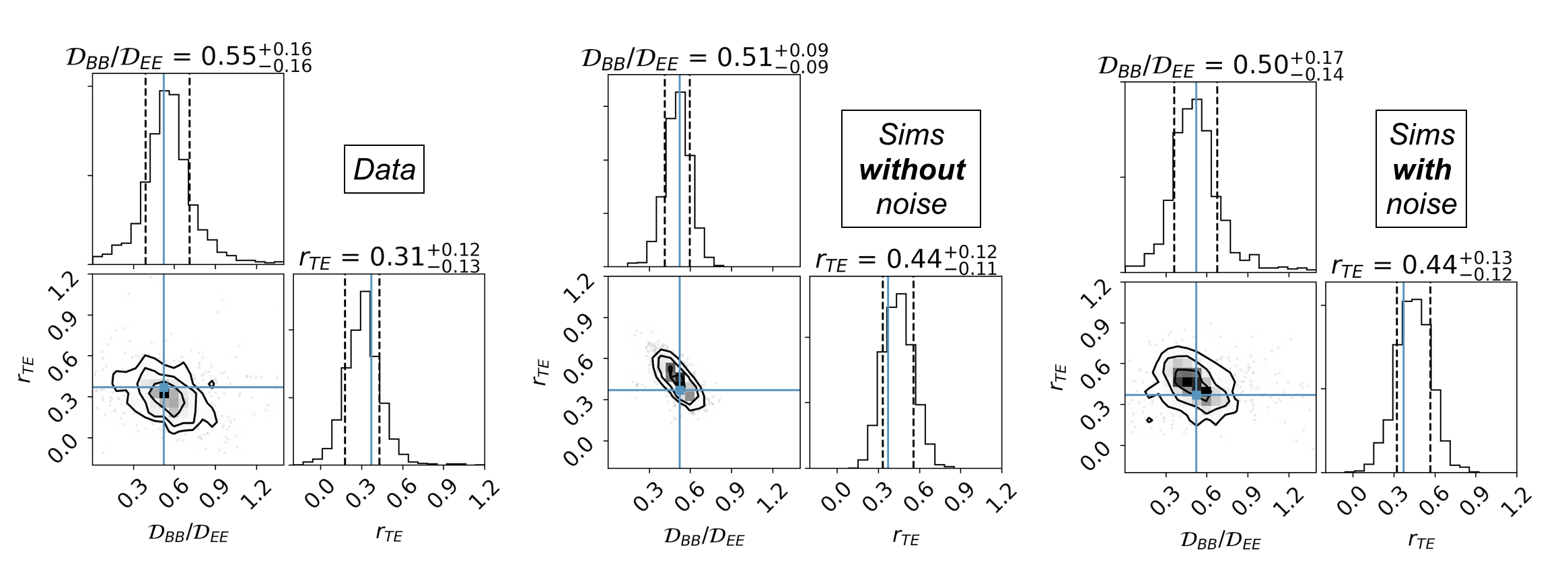
In this Appendix we test the methodology described in Sect. 3.2, performing the same analysis on non-Gaussian simulations of the polarized sky, which have the property of reproducing the 1- and 2-point statistics of the Planck polarization data at high Galactic latitude (Planck Collaboration Int. XLIV 2016; Vansyngel et al. 2017). These simulations are stochastic models of polarized dust emission on the sphere. The method builds on the understanding of Galactic polarization in terms of the structure of the Galactic magnetic field and its coupling with interstellar matter and turbulence through a handful of parameters. The simulated maps do not correspond to Gaussian random fields as shown in Fig. 5 of Vansyngel et al. (2017).
We generate two sets of simulations, with and without a noise realization from Planck (including systematic effects), in which the input values of and are fixed to 0.36 and 0.52, respectively. Results can be seen in Fig. 8 for the simulated parameter against the observed . The effect of noise does not increase significantly the variance in the correlation plots, which is dominated by the intrinsic variance among the different sky patches in the simulations, as will be detailed in the following. Moreover, as expected, no dependence exists between the observed and the simulated . We also notice that, regardless of the multipole bin, the input values for the medians of (solid horizontal lines) are obtained in output. The same is found for the simulated and parameters where the input values are set to 0. These two parameters do not show any systematic decrease in the median values with scale as observed in the Planck data. Thus, we conclude that the decrease in the median values of and observed in the data, from large to small scale, cannot be caused by noise or by our methodology. We suggest that, unless residual (unknown) systematic effects in the data are present, the observed decrease may be true. However, due to the large scatter in the distributions of the observed and , it is not possible to quantify the significance of this statement.
In Fig. 9 we show 1D and 2D probability density functions for and for the observed and the simulated data, respectively, considering bin 2 and bin 3 together in order to increase the number statistics. The two parameters appear clearly anticorrelated both in the observations and in the simulations. From Eq. 5 in Vansyngel et al. (2017) the inverse dependence in the simulated spectra can be derived as , where and . The effect of noise smooths the anticorrelation between and , suggesting that the true anticorrelation in the Planck data is likely stronger. The spread about the mean values found in the noisy simulations allows us to statistically recover the observed data dispersion (see the standard deviations quoted in the figure), confirming that sample variance is a major responsible for the -- power fluctuations from patch to patch over the sky at least in the diffuse ISM. This result validates the simulations presented in Vansyngel et al. (2017) for the statistical description of the polarized properties of the diffuse ISM even in small sky patches. However, as proved by our work, a significant dependence of the parameters with column density for cm-2 is observed. This is not captured yet by any existing model.
Appendix B Cosmic variance per multiple bin
We show a figure that allows us to quantify the level of cosmic variance in each multipole bin used in the data analysis. Following Tegmark (1997), the cosmic variance can be estimated as
| (11) |
where is the sky fraction considered and related to the sky-patch size as , which in our case is ; and is the width of the -bin equal to 15, 40, 200, 500, and 1200 from bin 0 to bin 4 respectively. As shown in Fig. 10, neglecting bin 0 enables us to limit the level of cosmic variance per bin below 20%. Notice that this equation is not completely accurate for cross-spectra. In that case it would read . Moreover, this estimates are only valid in case of Gaussian random fields. The observed signal is not Gaussian, thus we expect a larger amount of variance per bin of a factor of a few (Vansyngel et al. 2017).