Meshfree Methods on Manifolds for Hydrodynamic Flows on Curved Surfaces: A Generalized Moving Least-Squares (GMLS) Approach.

We utilize generalized moving least squares (GMLS) to develop meshfree techniques for discretizing hydrodynamic flow problems on manifolds. We use exterior calculus to formulate incompressible hydrodynamic equations in the Stokesian regime and handle the divergence-free constraints via a generalized vector potential. This provides less coordinate-centric descriptions and enables the development of efficient numerical methods and splitting schemes for the fourth-order governing equations in terms of a system of second-order elliptic operators. Using a Hodge decomposition, we develop methods for manifolds having spherical topology. We show the methods exhibit high-order convergence rates for solving hydrodynamic flows on curved surfaces. The methods also provide general high-order approximations for the metric, curvature, and other geometric quantities of the manifold and associated exterior calculus operators. The approaches also can be utilized to develop high-order solvers for other scalar-valued and vector-valued problems on manifolds.

1 Introduction

Many investigations in fluid mechanics pose challenges related to resolving hydrodynamic flows on curved surfaces or in confined geometries. Examples include the transport of surfactants within bubbles and thin films [47, 104, 54, 16, 65], protein drift-diffusion dynamics within lipid bilayer membranes and cell mechanics [23, 39, 88, 71, 78, 83], and colloidal aggregation within fluid interfaces [19, 60, 30]. Additional examples include stratified models in atmospheric and ocean science which employ shallow water equations within topologically spherical shells [109] and subsurface models governing the flow of groundwater through fractures in porous rock providing intricate geometries formed from the crack surfaces [4, 20, 67, 36]. For these problems the fluid mechanics can often be formulated in terms of effective fields on two dimensional surfaces. In some cases these problems also can involve additional challenges of tracking an evolving geometry of the surface from the motion of the interface or even of tracking topological changes [91, 38, 89]. We shall consider here primarily the problem of resolving hydrodynamic flows for surfaces of static shape. Already in this case, challenges arise in formulating the hydrodynamic equations and numerical methods to take into account the contributions of the geometry.

There has been a lot of interest in developing numerical methods to solve Partial Differential Equations (PDEs) on manifolds. Broadly categorized, these include Finite Element Methods (FEMs)  [27, 11, 28, 25], Level Set Methods (LSMs) and Phase Field Methods (PFMs) [79, 93, 26, 14, 94, 89, 14, 26], Discrete Exterior Calculus Methods (DECMs) [22, 49], Finite Element Exterior Calculus Methods (FEECMs) [41, 9, 24], and other approaches [113, 43, 75, 102, 64, 62]. Each of these approaches have their strengths depending on the application addressed as well as having challenges. FEMs offer specialized high-order methods with robust behaviors for broad problem classes with often rigorous guarantees of accuracy and stability when mesh quality factors for the geometry can be ensured [17]. LSMs/PFMs provide an implicit representation of the geometry often more amenable to evolution and topological changes, but typically require sophisticated algorithms to track the interface, mitigate numerical diffusion, and recover quantities associated with the geometry and the scalar and vector fields on the surface [94, 89, 14, 26, 14, 111, 112]. The DECMs/FEECMs provide discretizations with desirable qualities for mechanics allowing for derivation of methods that have conservation of mass, momentum, and vorticity [73]. By their design for preserving geometric structure, DECMs/FEECMs are currently applied primarily in fluid mechanics to inviscid flows. While DECMs are elegant and very useful discretizations that have been applied successfully to many applications [72, 22, 73, 21], for some scientific calculations they are low order, have limited convergence analysis [29, 74], or are restricted to specialized surface operations presenting some challenges for general physical modeling [55, 15]. In each of these methods, there is also a reliance upon a sufficiently high quality rectified or curvi-linear mesh or grid to locally represent the surface geometry or surface fields. To complement these methods, we consider alternatives based on meshfree approaches for surface hydrodynamics and PDEs based on Generalized Moving Least Squares (GMLS) approximations [110].

We develop GMLS approaches to approximate differential operators on manifolds where the shape is represented as a point set that samples the geometry. We build on recent related work by Liang et al. who discretized the surface Laplace-Beltrami operator on manifolds [63]. We construct smooth continuous representations of the manifold by solving a collection of local least-squares problems over an approximating function space at each of the sample points to obtain local paramerizations. This approach captures the geometry in a manner similar to [98, 58, 50, 7]. We approximate the surface scalar fields, vector fields, and differential operators by solving another collection of related local least-squares problems that make use of the geometric reconstructions. In conjunction, these provide general methods for obtaining high-order approximations of the manifold shape, operators arising in differential geometry, and operators of differential equations. We use exterior calculus for generalizing operations from vector calculus and techniques from mechanics to the manifold setting. This provides a convenient way to formulate incompressible hydrodynamic equations for flows on curved surfaces and related GMLS approximations. We also use these approaches to show in general how equations and related solvers can be formulated in terms of vector potentials facilitating development of other physical models with constraints and numerical methods.

We also mention there are many existing meshfree approaches for solving PDEs. These may be characterized broadly by the underlying discretizations. This includes Radial Basis Functions (RBFs) [18], Smooth Particle Hydrodynamics (SPH) [42], and the approaches of Generalized Finite Differences / Moving Least Squares / Reproducing Kernel Particle Method (GFD/MLS/RKPM) [59]. While the majority of meshfree literature has concerned solution of PDEs in $\mathbb{R}^{d}$, significant recent work has focused on the manifold setting [62, 63, 84, 96, 75, 64, 5, 82, 40]. In the last decade, substantial work has been done to use RBFs to solve shallow-water equations on the sphere [33]. The meshfree setting is attractive particularly for building semi-Lagrangian schemes of interest in atmosphere science and other applications [96]. Significant work also has been done on RBF methods to obtain robust numerical methods for predictive simulations in [34, 32, 37] and for solving PDEs on manifolds without the need for local surface reconstructions in [97, 95]. Recent work on RBF-FD also includes methods for reaction-diffusion equations on surfaces and other PDEs [97, 61, 95] and related approaches in [82, 81, 35].

SPH approaches have also been introduce that offer attractive structure-preserving properties, particularly in conserving invariants of Lagrangian transport. However, in general it is not possible for SPH to simultaneously obtain conservation principles and a consistent discretization [107]. The MLS/RKPM/GFD approaches provide a compelling alternative by addressing accuracy issues through the explicit construction of approximations with polynomial reproduction properties and an accompanying rigorous approximation theory [110, 90]. However, it should be noted in many cases stability theory currently is still lacking. There have been several examples of successful discretizations for scalar surface PDEs in [100, 103].

In Generalized Moving Least Squares (GMLS) this approach is extended to enable the recovery of arbitrary linear bounded target functionals from scattered data [110, 70]. For transport and flow problems in $\mathbb{R}^{d}$, compatible GMLS methods have been developed in [106] which parallel the stability of compatible spatial discretization [8]. In the Euclidean setting, this has allowed for stable GMLS discretizations of Darcy flow in $\mathbb{R}^{d}$[108], Stokes flow in $\mathbb{R}^{d}$ [106], and fluid-structure interactions occurring in suspension flow [52]. In the recent work [105], is has been shown that the scheme developed by Liang et al. [63] to discretize the Laplace-Beltrami operator on manifolds admits an interpretation as a GMLS approximation. This unification enables extensions of the compatible staggered approach for Darcy in $\mathbb{R}^{d}$ [108] to the manifold setting [105].

We develop here related methods for discretizing the diverse collection of exterior calculus operators to obtain high-order solutions to PDEs on surfaces. We focus particularly on the case of developing methods for hydrodynamic flows on curved surfaces. We introduce background on the GMLS approximation approach in Section 2. In Section 3, we discuss how to use GMLS to reconstruct locally the manifold geometry from a point set representation, approximate quantities from differential geometry, and approximate operators that generalize vector calculus to the manifold setting. In Section 4, we show how exterior calculus approaches can be used to formulate equations for hydrodynamic flow on surfaces in a few different ways which facilitates development of alternative solvers. We discuss our numerical solvers for incompressible hydrodynamic flows in Section 5. Finally, in Section 6, we conclude with results discussing our investigations of the accuracy of the GMLS methods. In particular, we study convergence of the approximations for the operators on the manifold and the precision of our solvers for hydrodynamic flows on curved surfaces. Many of our methods can be adapted readily for approximating other scalar-valued and vector-valued PDEs on manifolds.

2 Generalized Moving Least Squares (GMLS)

The method of Generalized Moving Least Squares (GMLS) is a non-parametric functional regression technique for constructing approximations by solving a collection of local least-squares problems based on scattered data samples of the action of a target operator [110, 70, 70, 69]. These local problems are formulated by specifying a finite collection of functionals that probe features of the action of the target operator.

More specifically, consider a Banach space $\mathbb{V}$ and function $u\in\mathbb{V}$. We assume that $u$ is characterized by a scattered collection of sampling functionals $\Lambda(u):=\left\{\lambda_{j}(u)\right\}_{j=1}^{N}\subset\mathbb{V}^{*}$, where $\mathbb{V}^{*}$ is the dual of $\mathbb{V}$. Here, we shall primarily use sampling functionals that are point evaluations $\lambda_{i}(u)=\delta_{x_{i}}[u]=u(x_{i})$. We denote the collection of sample points as $\mathbb{X}_{h}:=\left\{\mathbf{x}_{j}\right\}_{j=1}^{N}$, where $h$ indicates the spatial resolution. We assume $\mathbb{X}_{h}\subset\Omega\subset\mathbb{R}^{d}$ for a compactly supported domain $\Omega$. We characterize the distribution of points by

$$h_{\mathbb{X},\Omega}=\underset{\mathbf{x}\in\Omega}{\sup}\underset{1\leq j\leq N}{\min}||\mathbf{x}-\mathbf{x}_{j}||_{2},\hskip 28.45274ptq_{\mathbb{X}}=\frac{1}{2}\underset{i\neq j}{\min}||\mathbf{x}_{i}-\mathbf{x}_{j}||_{2},\hskip 28.45274ptq_{\mathbb{X}}\leq h_{\mathbb{X},\Omega}\leq c_{qu}q_{\mathbb{X}}.$$ (1)

The $||\cdot||_{2}$ is the Euclidean norm, $h_{\mathbb{X},\Omega}$ is the fill distance, $q_{\mathbb{X}}$ is the separation distance of $\mathbb{X}_{h}$. The point set is called quasi-uniform if there there exists $c_{qu}>0$ in the last expression of equation 1. We shall assume $\mathbb{X}_{h}$ is quasi-uniform throughout, which is important in proving results about existence, convergence, and accuracy of GMLS [110, 70].

Consider a target linear functional $\tau_{\hat{\mathbf{x}}}$ at location $\hat{\mathbf{x}}$. For example, the point-evaluation of a differential operator $\tau_{\hat{\mathbf{x}}}=D^{\alpha}u(\hat{\mathbf{x}})$ with $\alpha$ the multi-index. To approximate such operators, we first solve using the samples a collection of local weighted $\ell_{2}$-optimization problems over a finite dimensional subspace $\mathbb{V}_{h}\subset\mathbb{V}$. In particular, we solve for $p^{*}\in\mathbb{V}_{h}$ with

$$p^{*}=\underset{{q\in\mathbf{V}_{h}}}{\mbox{argmin}}\sum_{j=1}^{N}\left(\lambda_{j}(u)-\lambda_{j}(q)\right)^{2}\omega(\lambda_{j},\tau_{\tilde{\mathbf{x}}}),\hskip 28.45274pt\omega(\lambda_{j},\tau_{\tilde{\mathbf{x}}})=\Phi(||\mathbf{x}_{j}-\tilde{\mathbf{x}}||_{2}).$$ (2)

The $\omega$ is a compactly supported positive function correlating information at the sample location $\mathbf{x}_{j}$ and the target location $\tilde{\mathbf{x}}$. Throughout, we take $\Phi$ to be radially symmetric with $\Phi(r)=\left(1-{r}/{\epsilon}\right)^{\bar{p}}_{+}$, where $(z)_{+}=\max\{z,0\}$ and $\bar{p}>0$ with the $\epsilon$ controlling the shape and support of $\omega$.

For the basis $\mathbb{V}_{h}=\mbox{span}\{\phi_{1},...,\phi_{\dim(\mathbb{V}_{h})}\}$, we denote by $\mathbb{P}(x)$ the vector whose $i^{th}$-entry is $[\mathbb{P}(x)]_{i}=\phi_{i}(x)$. The solution to equation 2 can be represented using a coefficient vector $\mathbf{a}(u)$ to express the GMLS approximation of $\tau_{\tilde{\mathbf{x}}}$ as

$$p^{*}=P(x)^{\intercal}\mathbf{a}(u),\hskip 28.45274pt\tau^{h}_{\tilde{\mathbf{x}}}(u)=\tau_{\tilde{\mathbf{x}}}(\mathbb{P})^{\intercal}\mathbf{a}(u).$$ (3)

Assuming that the collection of sampling functionals $\Lambda$ is unisolvent for $\mathbb{V}_{h}$, the GMLS estimate of $\tau_{\tilde{\mathbf{x}}}$ in equation 3 can be expressed as

$$\tau^{h}_{\tilde{\mathbf{x}}}(\phi)=\tau_{\tilde{\mathbf{x}}}(\mathbf{P})^{\intercal}\left(\Lambda(\mathbf{P})^{\intercal}\mathbf{W}\Lambda(\mathbf{P})\right)^{-1}\Lambda(\mathbf{P})^{\intercal}\mathbf{W}\Lambda(u).$$ (4)

The $\Lambda$ is called unisolvent over $\mathbb{V}_{h}$, if any element of $\mathbb{V}_{h}$ is uniquely determined by the collection of sampling functionals $\lambda_{j}$, here by the points in the support of $\omega$ [110].

We summarize the GMLS approximation approach in Figure 1. We use the following notation throughout

• $\tau_{\tilde{\mathbf{x}}}(\mathbf{P})\in\mathbb{R}^{\dim(V_{h})}$ denotes the vector with components consisting of the target functional applied to each of the basis functions $\phi_{k}$.

• $\mathbf{W}\in\mathbb{R}^{N\times N}$ denotes the diagonal weight matrix with entries $\left\{\omega(\lambda_{j},\tau_{\tilde{\mathbf{x}}})\right\}_{j=1}^{N}$.

• $\Lambda(\mathbf{P})\in\mathbb{R}^{N\times\dim(V_{h})}$ denotes the rectangular matrix whose $(j,k)$-entry is $\lambda_{j}(\phi_{k})$ corresponds to the application of the $j^{th}$ sampling functional $\lambda_{j}$ applied to the $k^{th}$ basis function $\phi_{k}$.

• $\Lambda(u)\in\mathbb{R}^{N}$ denotes the vector consisting of entries $\{\lambda_{j}(u)\}_{j=1}^{N}$ corresponding to the $N$ sampling functionals $\lambda_{j}$ applied to the function $u$.

We remark that an advantage of GMLS over traditional least-squares approaches is that to build up approximations it only requires information locally at nearby points. Algorithmically, the main expense in GMLS is in inverting over the base points $\tilde{\mathbf{x}}$ many separate small systems of dense normal equations given by equation 4. The GMLS approach is very well-suited to hardware acceleration and parallelization using packages such as the recent Compadre toolkit [56].

We shall consider here primarily the case when the target functional $\tau$ is selected to approximate point evaluations of either the function as in regression or of differential operators acting on manifolds. These approximations and estimates have relation to [77, 70, 110, 69]. For partial derivatives $\mathcal{D}^{\bm{\alpha}}$ in $\mathbb{R}^{d}$ with multi-index $\bm{\alpha}$, Mirzaei [70] proved the estimate

$$\|\mathcal{D}^{\bm{\alpha}}u-\mathcal{D}^{\bm{\alpha}}p^{*}\|_{2}\leq Ch^{m+1-|\alpha|}.$$ (5)

These reconstructions use $m^{th}-$order polynomials. We extend such approximations to the manifold setting to handle non-linear target functionals due to geometry-dependent terms. While Mirzaei’s analysis was not developed for the non-linear setting, we find empirically convergence rates manifest in our approximations similar to equation 5.

Remark.

We consider throughout quasi-uniform point sets of two-dimensional compact manifolds embedded in $\mathbb{R}^{3}$. It can be shown readily [110] that for the quasi-uniform Euclidean setting in $\mathbb{R}^{2}$ that there exists constants $c_{1},c_{2}>0$ such that $c_{1}h_{\mathbb{X},\Omega}\leq\frac{1}{\sqrt{n}}\leq c_{2}h_{\mathbb{X},\Omega}$, and thus the fill distance scales as $h\sim 1/\sqrt{n}$, where $n$ is the number of points. We shall use the notation $\bar{h}^{-1}:=\sqrt{n}$ to characterize the refinement level of the point set.

3 Geometric Reconstructions from the Point Set of the Manifold

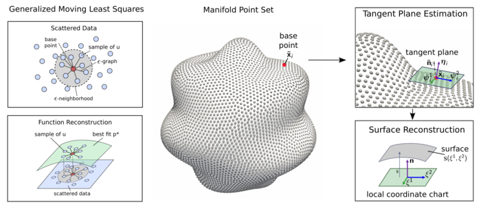
Figure 1: GMLS Approximation of Operators and Surface Reconstructions. A target functional $\tau_{\tilde{\mathbf{x}}}[u]$ is approximated using data within an $\epsilon$-neighborhood around the base point $\tilde{\mathbf{x}}$ (left-top). For values of $u$ the best fitting function $p^{*}\in\mathbb{V}_{h}$ is identified using the sampling functionals $\{\lambda_{j}\}$ for computing $\tau_{\tilde{\mathbf{x}}}^{h}[u]=\tau_{\tilde{\mathbf{x}}}[p^{*}]$ (left-bottom). For geometric reconstructions (center), a Principle Component Analysis (PCA) is used to find local parameterization of the surface of form $(\xi^{1},\xi^{2},s(\xi^{1},\xi^{2}))$ (top-right). The $s(\xi^{1},\xi^{2})$ and its derivatives are approximated by GMLS to obtain general geometric quantities of the manifold and approximate operators (bottom-right).

To formulate GMLS problems on manifolds, we must develop estimates of the metric tensor and other geometric quantities associated with the shape of the manifold. The metric tensor and geometric quantities are first extracted from the point cloud sampling of the manifold and then used to approximate the differential operators on the surface.

Consider a smooth manifold $\mathcal{M}\subset\mathbb{R}^{d}$ and assume a quasi-uniform point cloud sampling $\mathbb{X}_{h}\subset\mathcal{M}$. At each point $\mathbf{x}_{i}\in\mathbb{X}_{h}$, we shall construct an approximation to the tangent space $T_{\mathbf{x}_{i}}$ [110, 63]. At location $\mathbf{x}_{i}$, we use Principal Component Analysis (PCA) based on nearby neighbor points $\mathbf{x}_{j}$ such that $j\in\mathcal{N}_{i}$. The $\mathcal{N}_{i}=\mathcal{N}_{\epsilon}(\mathbf{x}_{i})=\{\mathbf{x}_{k}\,|\,\|\mathbf{x}_{k}-\mathbf{x}_{i}\|_{2}<\epsilon\}=\mathbb{X}_{h}\bigcap B_{\epsilon}(\mathbf{x}_{i})$ is the $\epsilon-$ball of samples around $\mathbf{x}_{i}$. To center the sample points for use in PCA, we define the centering point

$$\bar{\mathbf{x}}_{i}=\frac{1}{|\mathcal{N}_{i}|}\underset{j\in\mathcal{N}_{i}}{\sum}\mathbf{x}_{j}.$$ (6)

While in general $\bar{\mathbf{x}}_{i}\neq\mathbf{x}_{i}$, in practice these are typically close. We also refer to $\mathcal{N}_{i}=\mathcal{N}_{\epsilon}(\mathbf{x}_{i})$ as the patch of points at $\mathbf{x}_{i}$. For PCA we use for the empirical estimate of the covariance at $\mathbf{x}_{i}$

$$\mathcal{C}=\mbox{Cov}(\{\mathbf{x}_{j}\})=\frac{1}{|\mathcal{N}_{i}|}\underset{j\in\mathcal{N}_{i}}{\sum}\left(\mathbf{x}_{j}-\bar{\mathbf{x}}_{i}\right)\left(\mathbf{x}_{j}-\bar{\mathbf{x}}_{i}\right)^{\intercal}.$$ (7)

This provides a good estimate to the local geometry when $h_{\mathbb{X}}$ and $\epsilon$ are sufficiently small that the set of points $\mathcal{N}_{\epsilon}(\mathbf{x}_{i})$ is nearly co-planar. We estimate the tangent space $T\mathcal{M}_{\mathbf{x}_{i}}$ of the manifold using the $(d-1)$-largest eigenvectors of $\mathcal{C}$. These provide when $d=3$ a basis for the tangent plane that we denote by $\bm{\psi}^{1}_{i}$ and $\bm{\psi}^{2}_{i}$ and normalize to have unit magnitude. These also give the unit normal as $\bm{\eta}_{i}=\bm{\psi}^{1}_{i}\times\bm{\psi}^{2}_{i}$. We show the steps in the geometric reconstruction approach in Figure 1.

Remark.

It is important to note that the PCA-approach can arbitrarily assign an orientation in the reconstruction of the tangent space. This can have the undesirable property that neighboring patches have opposite orientations resulting in sign changes for some surface operators, such as the curl. In the general case, globally orienting the surface is a challenging NP-hard problem, as discussed in Wendland [110]. Many specialized algorithms have been proposed for this purpose which are efficient in practice, including front-marching and voronoi-based methods [6, 110]. We shall assume throughout that at each point $\mathbf{x}_{i}$ there is a reference normal $\tilde{\mathbf{n}}_{i}$ either determined in advance algorithmically or specified by the user. We take in our PCA procedures that the normals $\bm{\eta}_{i}$ are oriented with $\tilde{\mathbf{n}}_{i}^{T}\bm{\eta}_{i}>0$.

We use this approach to define a local coordinate chart for the manifold in the vicinity of the base point $\tilde{\mathbf{x}}=\mathbf{x}_{i}$. For this purpose, we take as the origin the base point $\mathbf{x}_{i}$ and use the tangent plane bases $\bm{\psi}_{i}^{1},\bm{\psi}_{i}^{2}$ and normal $\bm{\eta}_{i}$ obtained from the PCA procedure. We then define a local coordinate chart using the embedding map $\bm{\sigma}$

$$\bm{\sigma}(\xi^{1},\xi^{2};q)=\mathbf{x}_{i}+\xi^{1}\bm{\psi}_{i}^{1}+\xi^{2}\bm{\psi}_{i}^{2}+s(\xi^{1},\xi^{2})\bm{\eta}_{i}.$$ (8)

This provides a family of parameterizations in terms of local coordinates $(\xi^{1},\xi^{2})$, defined by choice of a smooth function $s$. Without loss of generality we could always define the ambient space coordinates so that locally at a given base point $\tilde{\mathbf{x}}$ we have $\bm{\sigma}=(\xi^{1},\xi^{2},s(\xi^{1},\xi^{2}))$. This can be interpreted as describing the surface as the graph of a function over the $(\xi^{1},\xi^{2})$-plane where $s$ is the height above the plane, see Figure 1. This parameterization is known as the Monge-Gauge representation of the manifold surface [76, 85], and we will use GMLS to approximate derivatives of $\bm{\sigma}$ through the following choices:

• We take for our sampling functionals $\Lambda=\{\lambda_{j}\}_{j=1}^{N}$ point evaluations $\lambda_{j}=\delta_{\mathbf{x}_{i}}$ at all points $\mathbf{x}_{j}$ in the $\epsilon$-ball neighborhood $\mathcal{N}_{i}$ of $\mathbf{x}_{i}$.

• We use the target functional $\tau^{[\bm{\alpha}]}$ as the point evaluation of the derivative $\mathcal{D}^{\bm{\alpha}}\bm{\sigma}$ at $\mathbf{x}_{i}$, where $\mathcal{D}^{\bm{\alpha}}$ denotes the partial derivative of $\bm{\sigma}$ in $\{\xi^{c}\}$ described by the multi-index $\bm{\alpha}$ [31].

• We take for the reconstruction space the collection of $m_{1}^{th}$-order polynomials.

• We use for our weighting function the kernel in equation 2 with support matching the parameter $\epsilon$ used for selecting neighbors in our reconstruction and for defining our $\epsilon$-graph on the point set.

We use these point estimates of the derivative of $\bm{\sigma}$ to evaluate non-linear functionals of $\bm{\sigma}$ characterizing the geometry of the manifold. Consider the metric tensor

$$g_{ab}=\langle\bm{\sigma}_{\xi^{a}},\bm{\sigma}_{\xi^{b}}\rangle_{g}.$$ (9)

The $\langle\mathbf{a},\mathbf{b}\rangle_{g}$ corresponds to the usual Euclidean inner-product $\mathbf{a}\cdot\mathbf{b}$ when the vectors $\bm{\sigma}_{\xi^{c}}=\partial\bm{\sigma}/\partial\xi^{c}$ are expressed in the basis of the ambient embedding space. Other geometric quantities can be similarly calculated from this representation once estimates of $\mathcal{D}^{\bm{\alpha}}\bm{\sigma}$ are obtained.

3.0.1 GMLS Approximation of Geometric Quantities

We now utilize these approaches to estimate Gaussian curvature, as a representative geometric quantity of interest. In Appendix A we provide detailed expressions for additional geometric quantities of interest which we will later need for approximating hydrodynamic flows on surfaces. To demonstrate in practice the convergence behavior of our techniques as the fill-distance is refined, we consider the four example manifolds shown in Figure 2.

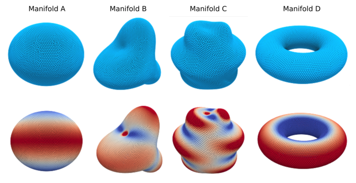
Figure 2: Point Set Representations of Manifolds (bottom). Manifold A is an ellipsoid defined by the equation ${x^{2}}/{a^{2}}+{y^{2}}/{b^{2}}+z^{2}=s_{0}^{2}$ with $a=1.2,b=1.2,s_{0}^{2}=1$. Manifold B is a radial manifold defined in spherical coordinates by $(\theta,\phi,r(\theta,\phi)$ where $r(\theta,\phi)=1+r_{0}\sin(3\phi)\cos(\theta)$ with $r_{0}=0.1$. Manifold C is a radial manifold defined in spherical coordinates by $(\theta,\phi,r(\theta,\phi)$ where $r(\theta,\phi)=1+r_{0}\sin(7\phi)\cos(\theta)$ with $r_{0}=0.1$. Manifold D is a torus defined by the equation $(s_{1}^{2}-\sqrt{x^{2}+y^{2}})^{2}+z^{2}=s_{2}^{2}$ with $s_{1}^{2}=0.7,s_{2}^{2}=0.3$. Estimated Gaussian curvature of the manifold (bottom). Each of the manifolds shown are represented by quasi-uniform point sets with approximately $n=10^{4}$ samples. For quasi-uniform sampling we expect the fill-distance $h$ to scale as $h\sim 1/\sqrt{n}$. When reporting our results, we use throughout the notation $\bar{h}^{-1}=\sqrt{n}$. We discuss further details of the point sampling of the manifolds in Appendix D.

We utilize the Weingarten map $\mathbf{W}=\mathbf{I}^{-1}\mathbf{II}$ to estimate the Gaussian curvature via the formula $K=\det(\mathbf{W})$ when using the GMLS estimate of $\bm{\sigma}_{\xi^{c}}$ to calculate $\mathbf{I}$ and $\mathbf{II}$, see Appendix A. We investigate the convergence of the estimated curvature for the manifolds A-D as the point sampling resolution increases in Table 1. We show the estimated curvature on the surface for each of the manifolds in Figure 2. We find our GMLS methods with $m=6$ yields approximations having $5^{th}$-order accuracy. While there is currently no convergence theory for our non-linear estimation procedure, the results for $k=2$ for Gaussian Curvature are consistent with the suggestive predictions $m+1-k$ of equation 5.

	Manifold A		Manifold B		Manifold C				Manifold D
h	$\ell_{2}$-error	Rate	$\ell_{2}$-error	Rate	$\ell_{2}$-error	Rate		h	$\ell_{2}$-error	Rate
0.1	2.1351e-04	-	1.1575e-01	-	1.2198e-01	-		.08	5.5871e-02	-
0.05	3.0078e-06	6.07	1.6169e-02	2.84	4.7733e-03	4.67		.04	6.5739e-04	6.51
0.025	5.3927e-08	5.77	8.3821e-04	4.26	1.6250e-04	4.88		.02	1.3418e-05	5.67
0.0125	1.1994e-09	5.48	2.3571e-05	5.14	4.5204e-06	5.17		.01	3.1631e-07	5.37

Table 1: Convergence of GMLS Approximation of the Gaussian Curvature $K$. The GMLS reconstruction of the manifold is used with polynomial order $m_{1}=6$. Our GMLS methods involve operations with $k_{1}=2^{nd}$-order differentiation. We find $\leavevmode\nobreak\ \sim 5^{th}$-order asymptotic convergence rate. The target sampling distance $h$ is discussed in Appendix D. The estimated Gaussian curvature for each manifold is shown in Figure 2.

3.1 Generalizing the Differential Operators of Vector Calculus to Manifolds using Exterior Calculus

The differential operators of vector calculus utilized in continuum mechanics formulations such as the grad, div, curl can be extended to corresponding operators on general manifolds. Differential operators on manifolds are notorious for having complicated notations when expressed in local coordinates [1]. We aim for a less coordinate-centric description of the methods and operators by utilizing approaches from exterior calculus. For this purpose, we utilize the operators of exterior calculus given by the Hodge star $\star$, exterior derivative $\mathbf{d}$, and vector to co-vector isomorphisms $\flat,\sharp$ (definitions below). Operators extend to the context of general manifolds acting on scalar fields $f$ and vector fields $\mathbf{F}$ as

$$\begin{array}[]{ll}{\mbox{grad}}_{\mathcal{M}}(f)=[\mathbf{d}f]^{\sharp},&{\mbox{div}}_{\mathcal{M}}(\mathbf{F})=-(-\star\mathbf{d}\star\mathbf{F}^{\flat})=-\bm{\delta}\mathbf{F}^{\flat},\\ {\mbox{curl}}_{\mathcal{M}}(\mathbf{F})=-\star\mathbf{d}\left[\mathbf{F}^{\flat}\right],&{\mbox{curl}}_{\mathcal{M}}(f)=\left[-\star\mathbf{d}f\right]^{\sharp}.\end{array}$$ (12)

We define $\bm{\delta}=(-\star\mathbf{d}\star)$ which is referred to as the co-differential. To define $\mathbf{d}$ the exterior derivative and $\star$ the Hodge star, we consider the tangent bundle $\mathcal{TM}$ of the manifold and its dual co-tangent bundle $\mathcal{TM}^{*}$. The tangent bundle defines the spaces for scalar fields, vector fields, and more generally rank $m$ tensor fields over the manifold. The co-tangent bundle is the space of duals to these fields. The co-tangent bundle can be viewed as the space of differential forms of order $0$, $1$, and $m$.

We denote vector fields and contravariant tensors using the notation $\mathbf{a}=a^{i_{1}\ldots i_{k}}\partial_{i_{1}}\cdots\partial_{i_{k}}$. We use $\partial_{i_{k}}$ to denote the basis vector $\partial_{i_{k}}=\partial\bm{\sigma}/\partial_{x^{i_{k}}}$ and tensor product these together to represent vectors and tensors for the choice of coordinates $\mathbf{x}=(x^{1},x^{2},\ldots,x^{d})$. We denote a differential $k$-form as $\bm{\alpha}=(1/k!)\alpha_{i_{1},\ldots,i_{k}}\mathbf{d}\mathbf{x}^{i_{1}}\wedge\cdots\mathbf{d}\mathbf{x}^{i_{k}}$. The $\wedge$ denotes the wedge-product of a tensor [1]. We use the convention here with $1/k!$ to allow summations over all permutations of the index values for $i_{1},\ldots,i_{k}$. A more detailed discussion of tensor calculus on manifolds can be found in [1].

We formulate the generalized operators in terms of the co-vectors (differential forms) $f^{\flat}$ and $\mathbf{F}^{\flat}$. We use that in the case of a scalar field we have quantitatively at each point $f=f^{\flat}$ [1]. The isomorphisms $\flat,\sharp$ mapping between the vector and co-vector spaces is given by

$$\mathbf{a}^{\flat} = (1/k!)g_{i_{1},\ell_{1}}\cdots g_{i_{k},\ell_{k}}a^{\ell_{1}\ldots\ell_{k}}\mathbf{d}\mathbf{x}^{i_{1}}\wedge\cdots\mathbf{d}\mathbf{x}^{i_{k}}$$ (13)

$$\bm{\alpha}^{\sharp} = (1/k!)g^{i_{1},\ell_{1}}\cdots g^{i_{k},\ell_{k}}\alpha_{\ell_{1}\ldots\ell_{k}}\partial_{\mathbf{x}^{i_{1}}}\cdots\partial_{\mathbf{x}^{i_{k}}}.$$ (14)

The exterior derivative $\mathbf{d}$ of a differential $k$-form $\bm{\alpha}$ is defined in terms of the coordinates $\mathbf{x}$ as

$$\mathbf{d}\bm{\alpha}=\frac{1}{k!}\frac{\partial}{\partial x^{j}}\alpha_{i_{1},\ldots,i_{k}}\mathbf{d}\mathbf{x}^{j}\wedge\mathbf{d}\mathbf{x}^{i_{1}}\wedge\cdots\mathbf{d}\mathbf{x}^{i_{k}}.$$ (15)

The Hodge star $\star$ is defined in terms of the coordinates $\mathbf{x}$ as

$$\star\bm{\alpha}=\frac{\sqrt{|g|}}{(n-k)!k!}\alpha^{i_{1},\ldots,i_{k}}\epsilon_{i_{1},\ldots,i_{k},j_{1},\ldots,j_{n-k}}\mathbf{d}x^{j_{1}}\wedge\cdots\wedge\mathbf{d}x^{j_{n-k}}.$$ (16)

Note the indices have been raised here for the $k$-form with $\alpha^{i_{1},\ldots,i_{k}}=g^{i_{1}\ell_{1}}\cdots g^{i_{k}\ell_{1}}\alpha_{\ell_{1},\ldots,\ell_{k}}$. The $\epsilon_{\ell_{1},\ldots,\ell_{n}}$ denotes the Levi-Civita tensor which gives the sign of the permutation of the indices $\ell_{1},\ldots,\ell_{n}$ and is otherwise zero [1].

This exterior calculus formulation allows us to provide a less coordinate centric description of the physics revealing in many cases more clearly the relationship of the continuum mechanics and role played by the geometry. This also has the advantage in analytic calculations of making expressions more concise and allowing more readily for generalization of identities and techniques employed from vector calculation [44, 99]. As for practical numerical calculations, we utilize this approach along with symbolic computation to generate offline the expressions needed for any choice of local coordinates on the manifold using equations 12– 16. This permits the efficient evaluation of these equations for any given choice of local coordinate using precompiled libraries for expressions. We give more details and show how this approach can be applied to the Laplace-Beltrami and Biharmonic operators in Appendix A.

3.1.1 GMLS Approximation of Differential Operators on Manifolds

Using these approaches we can perform GMLS estimates of the differential operators on the manifold. We consider the approximation of target functionals which may depend nonlinearly on estimates of the geometry. For example, the Laplace-Beltrami operator depends on the inverse metric tensor and can be expressed in local coordinates as

$$\Delta_{\tiny LB}\phi=\frac{1}{\sqrt{|g|}}\partial_{i}\left(\sqrt{|g|}g^{ij}\partial_{j}\phi\right).$$ (17)

We assume an estimate of $\mathbf{g}$ to be calculated at each point $\mathbf{x}_{i}$ following the approaches outlined in the previous sections. We then approximate the action of the operator on scalar and vector fields through the following GMLS approach. First, we find locally the best approximating reconstruction $\mathbf{P}$ of the scalar or vector field components on the manifold. In the second, we apply the target functional for the differential operator to $\mathbf{P}$ using geometric quantities from our initial GMLS reconstruction of the manifold. This can be expressed using the optimal coefficient vector $a_{\tilde{\mathbf{x}}}$ at $\tilde{\mathbf{x}}$ as

$$\tau^{h}_{\tilde{\mathbf{x}}}(\phi)=\tau_{\tilde{\mathbf{x}}}(\mathbf{P})^{\intercal}a_{\tilde{\mathbf{x}}}(u),\hskip 28.45274pta_{\tilde{\mathbf{x}}}(u)=\left(\Lambda(\mathbf{P})^{\intercal}\mathbf{W}\Lambda(\mathbf{P})\right)^{-1}\Lambda(\mathbf{P})^{\intercal}\mathbf{W}\Lambda(u).$$ (18)

In the general setting, the sampling functionals $\lambda_{j}$ may depend non-linearly on the geometric terms. In the current case using local point evaluations, the functionals $\lambda_{j}$ are linear.

We remark that the two components $a_{\tilde{\mathbf{x}}}(u)$ and $\tau_{\tilde{\mathbf{x}}}(\mathbf{P})$ encode different types of information about the approximation. The $\tau_{\tilde{\mathbf{x}}}(\mathbf{P})$ encodes the action of the target functional on the basis for the space $\mathbb{V}_{h}$. The $a_{\tilde{\mathbf{x}}}(u)$ encodes the reconstruction of the function $u$ by the best approximating function $p^{*}$ in $\mathbb{V}_{h}$ according to the best match between the sampling functionals $\lambda_{j}$ acting on $u$ and $p^{*}$, see equation 2. As a consequence, for each of the target operators $\tau$, the $a_{\tilde{\mathbf{x}}}(u)$ will not change since this term only depends on the function $u$. As a result, we need only compute fresh for each operator the $\tau_{\tilde{\mathbf{x}}}(\mathbf{P})$ which represents how the differential operator on the manifold acts on the function space $\mathbb{V}_{h}$.

As a summary, our GMLS approximation on the manifold involves the following steps

• Take $\Lambda=\{\lambda_{j}\}_{j=1}^{N}$ where $\lambda_{j}=\delta_{\mathbf{x}_{j}}$ are point evaluations with $\lambda_{j}\phi=\phi(\mathbf{x}_{j})$ for the $\mathbf{x}_{j}$ in the neighborhood $j\in\mathcal{N}_{i}$ around the point $\mathbf{x}_{i}$.

• For the target functionals $\tau$, treat the surface differential operators by utilizing for evaluation the parameterization and approximate metric tensor outlined in Section 3.0.1.

• For the reconstruction space $\mathbb{V}_{h}$, use the collection of $m_{2}^{th}$-order polynomials $p(x,y)$ over $\mathbb{R}^{2}$ where $m_{2}$ is an integer parameter for the maximum degree.

• For the weight function $\omega(\lambda_{j},\tau_{\mathbf{x}_{i}})=w(\|\mathbf{x}_{j}-\mathbf{x}_{i}\|)$, select a positive kernel $w(r)$ with support contained within an $\epsilon$-ball of $\mathbf{x}_{i}$. We also use this to construct an $\epsilon$-graph on the point set.

The reconstruction space $\mathbb{V}_{h}$ consists of polynomials of order $m_{2}$ which need not be chosen to be the same order $m_{1}$ as in the geometric reconstructions in Section 3, so in general $m_{2}\neq m_{1}$. However, in practice the operators on the manifold often involve differentiating geometric quantities which typically need $m_{1}\geq m_{2}$ to achieve convergence.

As an illustration of our GMLS approach, consider the Laplace-Beltrami operator. The other differential operators for the manifold follow similarly, but with more complicated expressions which we evaluate symbolically, see Appendix A. For the Laplace-Beltrami operator we have

$$\Delta_{\tiny LB}\phi=\frac{1}{\sqrt{|g|}}\partial_{i}\left(\sqrt{|g|}g^{ij}\partial_{j}\phi\right),\hskip 28.45274pt\tau_{\tilde{\mathbf{x}}}(\mathbf{P};\mathbf{g})=\frac{1}{\sqrt{|g|}}\partial_{i}\left(\sqrt{|g|}g^{ij}\partial_{j}\mathbf{P}\right).$$ (19)

On the left the Laplace-Beltrami operator is expressed in coordinates and on the right we have the GMLS approximation. The $\mathbf{P}$ represents the vector of basis functions of $\mathbb{V}_{h}$ and the differentials act component-wise.

Remark.

It is necessary to choose a reconstruction space $\mathbb{V}_{h}$ of sufficient richness that a differential operator on the manifold $\mathcal{L}_{\mathbf{g}}$ can be adequately represented. For instance, a differential operator of order $k$ should have a polynomial space of order $m_{2}$ satisfying $m_{2}\geq k$, as suggested by the bounds in equation 5. From these bounds we also do expect that higher-order convergence rates are possible when using larger degrees. This can yield computational efficiencies in achieving a desired level of accuracy, especially when treating smooth fields and low-order differential operators. However, it is important to note that larger choices of $m_{2}$ will necessitate that the neighborhoods defined by the weight function contain more points to ensure unisolvency and ultimately solvability of the GMLS problem.

We give additional details on our GMLS approach for specific operators in Appendix A.

4 Hydrodynamic Flows on Curved Surfaces

We formulate continuum mechanics equations for hydrodynamic flows on curved surfaces using approaches from the exterior calculus of differential geometry [66, 1]. This provides an abstraction that is helpful in generalizing many of the techniques of fluid mechanics to the manifold setting while avoiding many of the tedious coordinate-based calculations of tensor calculus. The exterior calculus formulation also provides a coordinate-invariant set of equations helpful in providing insights into the roles played by the geometry in the hydrodynamics. We provide a brief derivation of hydrodynamic equations here based on our prior work [99, 44, 45]. For additional discussion of the derivations for hydrodynamics on manifolds and related differential geometry, see [99, 45, 101, 66, 1].

4.1 Hydrodynamics in the Stokesian Regime

We consider the hydrodynamics in the quasi-steady-state Stokes regime where the flow is determined by a balance between the fluid shear stresses and the body force. The hydrodynamics in this regime can be expressed in covariant form as

$$\left\{\begin{array}[]{llll}\mu_{m}\left(-\bm{\delta}\mathbf{d}\mathbf{v}^{\flat}+2K\mathbf{v}^{\flat}\right)-\gamma\mathbf{v}^{\flat}-\mathbf{d}p&=&-\mathbf{b}^{\flat}\\ -\bm{\delta}\mathbf{v}^{\flat}&=&0.\end{array}\right.$$ (22)

The $\mathbf{v}^{\flat}$ is the surface fluid velocity, $p$ the surface presssure enforcing incompressibility, and $\mathbf{b}^{\flat}$ the surface force density driving the flow. The $\mu_{m}\left(-\bm{\delta}\mathbf{d}\mathbf{v}^{\flat}+2K\mathbf{v}^{\flat}\right)$ corresponds to the divergence of the internal shear stress of the surface fluid, and $-\bm{\delta}\mathbf{v}^{\flat}=0$ expresses the incompressibility constraint. The $\mu_{m}$ gives the surface fluid viscosity. It is worth pointing out that the surface shear stress has a dependence not only on the usual gradients in the velocity field but also the Gaussian Curvature $K$ of the surface. This can lead to interesting flow phenomena on curved surfaces and significant differences with respect to flat surfaces, as discussed in [99, 45, 10, 46].

We remark that the $-\gamma\mathbf{v}^{\flat}$ serves as our model for the coupling between the surface flow and bulk three-dimensional surrounding fluid. More sophisticated models also can be formulated, but for general geometries this requires development of a separate solver for the bulk three-dimensional surrounding fluid which we shall consider in future work. It is important in physical models to have some form of dissipative traction stress with the surrounding bulk fluid since this provides a crucial dissipative mechanism that suppresses the otherwise well-known Stokes paradox that arises in purely two-dimensional fluid equations [2, 12, 45, 92, 87]. Additional discussions of equation 22 and its derivation can be found in [45, 99].

4.2 Vector Potential Formulation for Incompressible Flows and Hodge Decomposition

We generalize approaches from fluid mechanics to the context of manifolds to handle the incompressibility constraint in equation 22. We reformulate equation 22 using the Hodge decomposition and a vector potential $\phi$ that ensures the generated velocity fields are incompressible. By utilizing this gauge to describe the physics we can avoid the challenges in numerical methods associated with having to enforce explicitly the incompressibility constraint. We use a surface Hodge decomposition of the fluid velocity field that can be expressed using the exterior calculus as

$$\mathbf{v}^{\flat}=\mathbf{d}\psi+\bm{\delta}\phi+\mathbf{h}.$$ (23)

The $\psi$ is a $0$-form, $\phi$ is a $2$-form, and $\mathbf{h}$ is a harmonic $1$-form on the surface with respect to the Hodge Laplacian $\Delta_{H}\mathbf{h}=\left(\bm{\delta}\mathbf{d}+\mathbf{d}\bm{\delta}\right)\mathbf{h}=0$. The first term $\mathbf{d}\psi$ captures the curl-free component of the velocity field, the second term $\bm{\delta}\phi$ the divergence-free component of the velocity field, and the third term an additional harmonic part that arises from the topology of the manifold. In the Euclidean setting only the first two terms typically play a role since the harmonic term in this case is often a trivial constant and with decay conditions at infinity the constant is zero.

In the non-Euclidean setting there can be many non-trivial harmonic $1$-forms. The number is determined by the dimensionality of the null-space of the Hodge Laplacian which depends on the topology of the manifold [53]. As a consequence, we have for different topologies that the richness of the harmonic differential forms $\mathbf{h}$ appearing in equation 23 will vary. Fortunately, in the case of spherical topology the surface admits only the trivial harmonic $1$-forms $\mathbf{h}=\bm{0}$ making this manifold relatively easy to deal with in our physical descriptions. As we shall discuss, for more general topologies our incompressibility gauge descriptions will require solving additional coupled equations in order to resolve the non-trivial harmonic contributions. We shall focus here primarily on the case of manifolds having spherical topology and pursue in future work development of these additional numerical solvers needed for the harmonic component.

We consider incompressible velocity fields $\mathbf{v}^{\flat}$ on manifolds having spherical topology. When applying the co-differential $\bm{\delta}$ to equation 23 and utilizing the incompressibility constraint in equation 22, we have $\bm{\delta}\mathbf{v}^{\flat}=\bm{\delta}\mathbf{d}\psi=\Delta_{H}\psi=0$. For spherical topology this requires $\psi=C$ and $\mathbf{d}\psi=0$. As a consequence, we can express the incompressible hydrodynamic velocity fields as

$$\mathbf{v}^{\flat}=\bm{\delta}\phi.$$ (24)

From the co-differential operator $\bm{\delta}$ defined in Section 3.1, we see that $\phi$ is a $2$-form on the two-dimensional surface. In practice, we find it more convenient to express $\mathbf{v}^{\flat}$ in terms of an operation on a $0$-form (scalar field) which can be done using the Hodge star to obtain $\Phi=\star\phi$. Using the identity of the Hodge star that $\star\star=(\star)^{2}=-1$ for 2-manifolds. This gives $\phi=-\star\Phi$. This allows us to express incompressible hydrodynamic flow fields as

$$\mathbf{v}^{\flat}=-\star\mathbf{d}\Phi.$$ (25)

We refer to $\Phi$ as the vector potential since it serves as a potential to generate vector fields $\mathbf{v}$. This can be interpreted as a generalized curl operation as in equation 12 applied to a scalar field which intrinsically generates divergence-free vector fields $\mathbf{v}$ . This approach generalizes the vorticity-stream formulation of fluid mechanics [3] to the manifold setting. We use this to reformulate the hydrodynamic equations in terms of unconstrained equations in terms of $\Phi$.

4.2.1 Biharmonic Formulation of the Hydrodynamics

We reformulate the hydrodynamics equations 22 in terms of an unconstrained equation for the vector potential $\Phi$. We substitute equation 25 into equation 22 and apply the generalized curl operator $\mbox{curl}_{\mathcal{M}}=-\star\mathbf{d}$ to both sides. This gives the biharmonic hydrodynamic equations on the surface

$$-\mu_{m}\Delta_{H}^{2}\Phi-\gamma\Delta_{H}\Phi-2\mu_{m}(-\star\mathbf{d}(K(-\star\mathbf{d})))\Phi = -\star\mathbf{d}\mathbf{b}^{\flat}.$$ (26)

The $\mu_{m}$ is the surface shear viscosity, $\gamma$ the drag with the surrounding bulk fluid, and $K$ the Gaussian curvature of the manifolds. The $\mathbf{b}^{\flat}$ is the covariant form for the body force acting on the fluid. We see the pressure term no longer plays a role relative to equation 22.

The Hodge Laplacian now acts on $0$-forms as $\Delta_{H}\Phi=\bm{\delta}\mathbf{d}\Phi$ and is related the surface Laplace-Beltrami operator by $\Delta_{H}\Phi=-\Delta_{LB}\Phi$. This provides for numerical methods a particularly convenient form for the fluid equations since it only involves solving for a scalar field $\Phi$ on the surface. However, this does have the drawback that for handling the incompressibility constraint this way we now need to solve a biharmonic equation on the surface. We shall refer in our numerical methods to this approach to the hydrodynamics as the biharmonic formulation.

We remark that our approach can be related to classical methods in fluid mechanics by viewing our operator $-\star\mathbf{d}$ as a type of curl operator that is now generalized to the manifold setting. The $\Phi$ serves the role of a vector potential for the flow [2, 12, 57]. The velocity field of the hydrodynamic flows $\mathbf{v}$ is recovered from the vector potential $\Phi$ as $\mathbf{v}^{\flat}=-\star\mathbf{d}\Phi$. We obtain the velocity field $\mathbf{v}=\mathbf{v}^{\sharp}=\left(-\star\mathbf{d}\Phi\right)^{\sharp}$ using equation A.3 and the isomorphisms $\sharp$ between co-vectors and vectors discussed in Section 3.1. Additional discussion of this formulation of the hydrodynamics can be found in [99, 45].

4.2.2 Split Formulation of the Hydrodynamics

While the equation 26 is expressed in terms of biharmonic operators, for numerical purposes we can reformulate the problem by splitting it into two sub-problems each of which only involve the Hodge Laplacian. This is helpful since for our numerical methods this would require us to only need to resolve second order operators with our GMLS approximations. This has the practical benefit of greatly reducing the size of the GMLS stencil sizes ($\epsilon$-neighborhoods) required for unisolvency for the operator as discussed in Section 2.

We reformulate the hydrodynamic equations by defining $\Psi=\Delta_{H}\Phi$, which allows us to split the action of the fourth-order biharmonic operator into two equations involving only second- order Hodge Laplacian operators as

$$-\mu_{m}\Delta_{H}\Psi-\gamma\Psi-2\mu_{m}(-\star\mathbf{d}(K(-\star\mathbf{d})))\Phi = -\star\mathbf{d}\mathbf{b}^{\flat}.$$ (27)

$$\Delta_{H}\Phi-\Psi = 0.$$ (28)

As we shall discuss, the lower order of the differentiation has a number of benefits even though we incur the extra issue of dealing with a system of equations. This reformulation results in less sensitivity to errors in the underlying approximations in the GMLS reconstructions of the geometry and surface fields. This reformulation also requires much less computational effort and memory when assembling the stiffness matrices since the lower order permits use of smaller $\epsilon$-neighborhoods to achieve unisolvency as discussed in Section 2. We refer to this reformulation of the hydrodynamic equations as the split formulation.

For a further discussion of these surface hydrodynamics equations, related derivations, and physical phenomena see [99, 45].

5 Computational Methods and Numerical Solvers

We develop numerical methods to solve equations 26 or 27 for the velocity field of hydrodynamic flows on surfaces using the GMLS approximations of Section 2 and 3. We briefly discuss the overall steps used in our numerical methods. We formulate the hydrodynamics using a vector-potential formulation to obtain a gauge that intrinsically enforces the incompressibility constraints of the flow appearing in equation 22. For steady-state hydrodynamic flows, we derived conditions for the vector potential of the flow resulting in equation 26. We summarize the steps used in our solution approach in Figure 3.

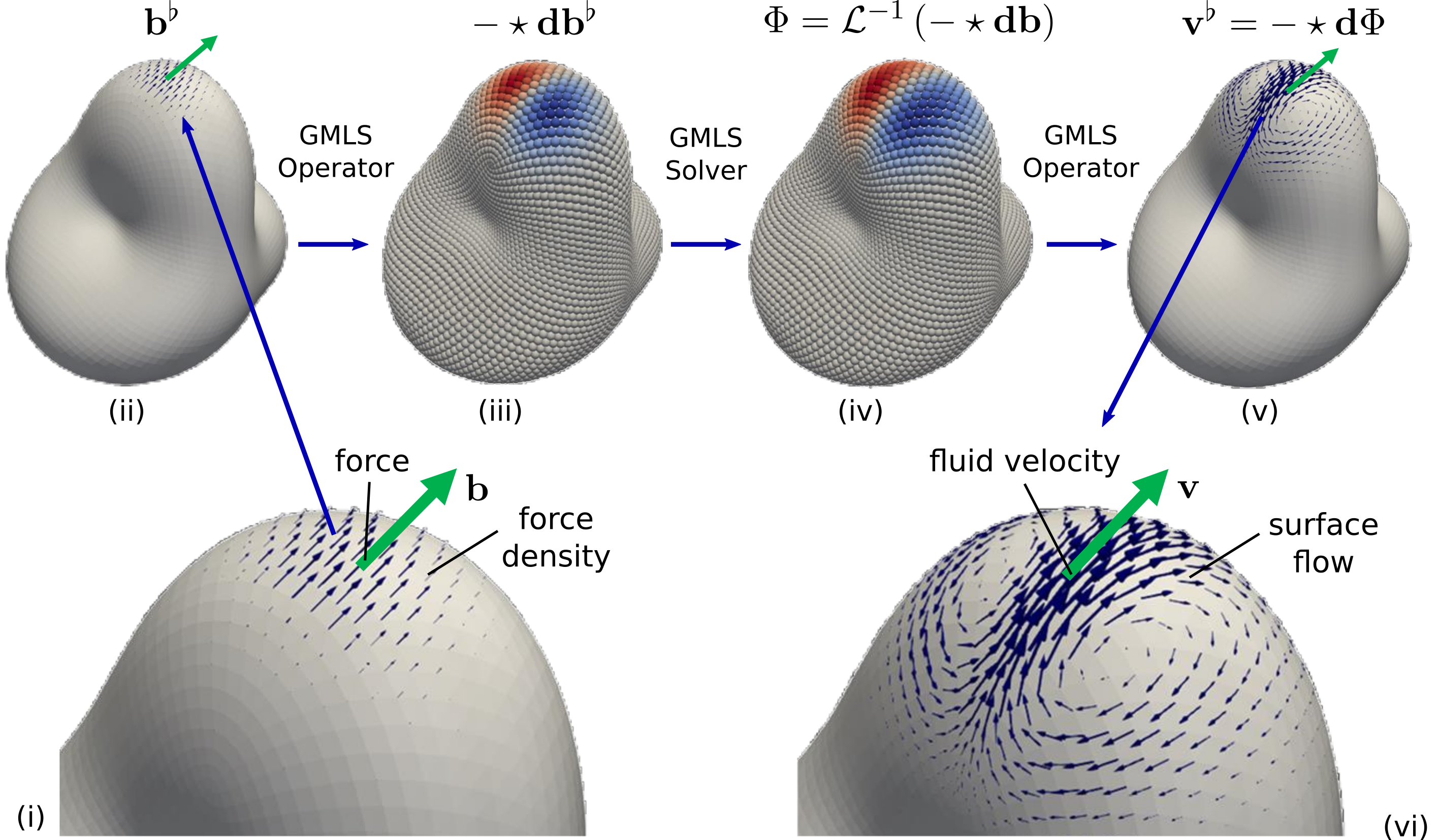
Figure 3: Steps in the Numerical Methods for the Surface Hydrodynamic Flows. For a given body force density or stresses $\mathbf{b}$ acting on the surface fluid we convert the fields to covariant form $\mathbf{b}^{\flat}$, shown in (i),(ii). To handle incompressibile flows, we convert all fields to a divergence-free gauge using the generalized surface curl $-\star\mathbf{d}\mathbf{b}^{\flat}$, shown in (iii). We solve for the vector potential $\Phi$ of the surface hydrodynamic flow using equations 26 or 27 and our GMLS collocation methods for the differential operators, shown in (iv). We construct the covariant form of the velocity field of the hydrodynamic flow response using the generalized surface curl $\mathbf{v}^{\flat}$, shown in (v). We obtain our final results by converting the covariant form $\mathbf{v}^{\flat}$ to the velocity field by $\mathbf{v}=\left(\mathbf{v}^{\flat}\right)^{\sharp}$. This yields the surface hydrodynamic flow shown in (vi).

To determine numerically the hydrodynamic flow in response to a body force density $\mathbf{b}$ acting on the surface fluid, we first convert force fields into co-variant form $\mathbf{b}^{\flat}$. We next use our exterior calculus formulation of the generalized curl to obtain the corresponding vector-potential for the body force $\Psi=\mathcal{C}_{1}\mathbf{b}^{\flat}$ where $\mathcal{C}_{1}=-\star\mathbf{d}$ acts on $1$-forms. We numerically compute $\Psi=\tilde{C}_{1}\mathbf{b}^{\flat}$ where $\tilde{C}_{1}$ is our GMLS approximation of the curl operator $\mathcal{C}_{1}$ discussed in Section 3.1.1 and Appendix A.3.

We can now utilize equation 26 to specify the differential equation for the steady-state velocity response. We use GMLS to assemble in strong form a stiffness matrix $A$ using a collocation approach. The full differential operator that appears on the left-hand-side is computed at each base point $\tilde{\mathbf{x}}$ of the point set of the manifold. This results in the system of equations linear in $\tilde{\mathbf{\Phi}}$

$$A\tilde{\mathbf{\Phi}}=\tilde{C}_{0}\mathbf{b}.$$ (29)

We solve the large linear system using GMRES with algebraic multigrid (AMG) preconditioning.

The velocity field is given from the vector potential $\Phi$ by the generalized surface curl operator $\mathbf{v}^{\flat}=\mathcal{C}_{0}\Phi$, where $\mathcal{C}_{0}=-\star\mathbf{d}$ acts on $0$-forms. From the solution $\tilde{\mathbf{\Phi}}$ of equation 29, we construct numerically the co-variant velocity field of the flow using $\tilde{\mathbf{v}}^{\flat}=\tilde{C}_{0}\tilde{\mathbf{\Phi}}$. The $\tilde{C}_{0}$ is our GMLS approximation of the generalized curl operator $\mathcal{C}_{0}$ discussed in Section 3.1. Finally, using the metric tensor obtained from the GMLS reconstruction, we obtain the surface velocity field $\tilde{\mathbf{v}}$ by converting the covariant field $\mathbf{v}^{\flat}$ into the contravariant field by $\tilde{\mathbf{v}}=\left(\tilde{\mathbf{v}}^{\flat}\right)^{\sharp}$. For more details on this approach and operations see Appendix A.3. We use this approach to numerically compute incompressible hydrodynamic flows in response to applied driving forces or stresses acting on the surface fluid. We remark that our approach can also be combined with other computational methods and solvers to compute coupling to bulk three dimensional hydrodynamics or more generally for resolving other physical systems and interactions that occur at interfaces.

The Compadre toolkit [56] was used to solve the GMLS problems. The toolkit provides domain decomposition and distributed vector representation of fields as well as global matrix assembly. The linear equations were solved through iterative block solvers (Belos [13]), block preconditioners (Teko) and AMG preconditioning (MueLu [86, 51]), within the Trilinos software framework [48].

6 Results

6.1 Convergence Results for Operators on Manifolds based on GMLS Geometric Reconstructions

We investigate the convergence of the GMLS approximation of the operators required to solve the hydrodynamic equations in Section 4. It is important to note that our target functionals have a non-linear dependence on the geometry resulting in contributions from two different GMLS approximations. First, the GMLS reconstruction of the geometry of the manifold and associated associated geometric quantities. Second, the GMLS approximation of differential operators acting on the surface scalar and vector fields.

Our solvers for the surface hydrodynamic flows of equation 26 and 27 use the following operators: Laplace-Beltrami $\mathcal{L}_{LB}=-\Delta_{H}=-\mathbf{d}\bm{\delta}$, Biharmonic $\mathcal{L}_{BH}=\mathcal{L}_{LB}^{2}=\Delta_{H}^{2}$,Curvature $\mathcal{L}_{K}=curl_{\mathcal{M}}\left(K\cdot curl_{\mathcal{M}}\right)=-\star\mathbf{d}\left(K\cdot(-\star\mathbf{d}\right)$, Surface-Curl-$0$-Forms $\mathcal{C}_{0}$,$\mathcal{L}_{C0}=\mbox{curl}_{\mathcal{M}}\Phi=-\star\mathbf{d}_{0}$, Surface-Curl-$1$-Forms $\mathcal{C}_{1}$,$\mathcal{L}_{C1}=\mbox{curl}_{\mathcal{M}}\mathbf{v}=-\star\mathbf{d}_{1}$. In the split formulation of equation 27, this simplifies without the need for $\mathcal{L}_{BH}$.

To approximate each of the operators using GMLS, we use point samples within a distance $\epsilon$ from the target point $x_{i}$. For the local optimization problems to determine the polynomial of degree $m$, a minimum of $n_{p}=\binom{m+2}{2}$ points are needed per neighborhood. To find such an $\epsilon$, we sweep through the points and either increase or decrease the initial guess $\epsilon_{0}$ by a factor $\beta_{*}$. This is done so that the $\epsilon=\beta_{*}^{k}\epsilon_{0}$ can be used globally to generate neighborhoods with at least $\alpha_{*}n_{p}$ points in each of them, where $\alpha_{*}\geq 1$ is a tune-able parameter for calculations. This is used to determine the polynomial representation $p^{*}$. In practice, the factor $\alpha_{*}$ is used to ensure significantly more points are in neighborhoods than are strictly needed which helps to provide additional robustness in calculations. We use throughout $\alpha_{*}=2.8$ and $\beta_{*}=2$.

To study the accuracy of our GMLS approximation of these operators, we investigate the case of the test scalar field $\Phi(\mathbf{X})=\Phi(x,y,z)=z(x^{4}+y^{4}-6x^{2}y^{2})$ and test vector field $\mathbf{v}^{\flat}=\mathcal{C}_{0}\Phi=-\star\mathbf{d}_{0}\Phi$. We have chosen $\Phi(x,y,z)$ to be a smooth continuation of a spherical harmonic mode to the full space $\mathbb{R}^{3}$. Since our manifolds $\mathcal{M}$ are smooth, we obtain a smooth surface scalar field by evaluation of $\Phi(\mathbf{X})$ at the surface (i.e. using the inclusion map $\iota:\mathbb{R}^{3}\xhookrightarrow{}\mathcal{M}$ with $\Phi(\mathbf{x})=\iota_{\mathbf{x}}\Phi(\cdot)$). This provides a way to define surface scalar fields and vector fields without the need for local coordinate charts on the manifold.

We investigate the accuracy of the GMLS approximation of these operators. We study the $\ell^{2}$-errors

$$\epsilon_{op0}=\left\|\tilde{L}_{\mathbf{g}}\Phi-\mathcal{L}_{\mathbf{g}}\Phi\right\|_{2},\hskip 28.45274pt\epsilon_{op1}=\left\|\tilde{L}_{\mathbf{g}}\mathbf{v}-\mathcal{L}_{\mathbf{g}}\mathbf{v}\right\|_{2}.$$ (30)

The $\ell^{2}$-norm is computed by averaging the error over all $n$ sample points of the manifold $\|u-v\|_{2}^{2}=\frac{1}{n}\sum_{i}\left(u(\mathbf{x}_{i})-v(\mathbf{x}_{i})\right)^{2}$. The $\tilde{L}_{\mathbf{g}}$ denotes the numerical GMLS approximation of the operator $\mathcal{L}_{\mathbf{g}}$. In practice, for comparison with the GMLS results in the convergence studies, we evaluate to high precision the action of the operators $\mathcal{L}_{\mathbf{g}}$ by using symbolic calculations using SymPy [68].

Using this approach, we investigate the accuracy of the GMLS approximation of the operators for each of the manifolds in Tables 2– 4. We estimate approximate convergence rates by fitting using in a log-log scale the error between the reported $h$ value and the previous $h$ value. While we do not have theory given that the operators have a non-linear dependence on the manifold geometry, for operators of order $k$ and GMLS approximation of order $m$ we do have the suggestive predictions from equation 5 that the convergence be order $m+1-k$. Since our GMLS methods involve approximations both of the geometry and the surface fields, for purposes of the comparisons we take $k=\max(k_{1},k_{2})$ and $m=\max(m_{1},m_{2})$. The $k_{1}$ denotes the order of the differentiation involved in obtaining the quantities associated with the geometry and $k_{2}$ with the order of differentiation of the surface fields. The $m_{1},m_{2}$ are the polynomial orders used for the approximations for the manifold geometry and surface fields, as discussed in Section 2.

	Manifold A		Manifold B		Manifold C				Manifold D
h	$\ell_{2}$-error	Rate	$\ell_{2}$-error	Rate	$\ell_{2}$-error	Rate		h	$\ell_{2}$-error	Rate
0.1	4.2208e-04	-	2.2372e-02	-	1.3580e-01	-		.08	4.7880e-02	-
0.05	7.503e-06	5.74	1.2943e-03	4.11	4.8597e-03	4.80		.04	5.5252e-04	6.54
0.025	1.8182e-07	5.34	5.8300e-05	4.46	1.2928e-04	5.24		.02	1.3877e-05	5.36
0.0125	4.8909e-09	5.21	1.7364e-06	5.06	3.7508e-06	5.11		.01	3.7568e-07	5.17

Table 2: Convergence of GMLS Approximation of the Laplace-Beltrami Operator $\mathcal{L}_{LB}$. We use GMLS with ($k=2,m=6)$ and find the methods have $\sim 5^{th}$-order asymptotic convergence. The target sampling distance $h$ is discussed in Appendix D.

	Manifold A		Manifold B		Manifold C				Manifold D
h	$\ell_{2}$-error	Rate	$\ell_{2}$-error	Rate	$\ell_{2}$-error	Rate		h	$\ell_{2}$-error	Rate
0.1	1.7177e-01	-	1.1102e+01	-	6.9226e+01	-		.08	4.0566e+01	-
0.05	1.0768e-02	3.94	2.1455e+00	2.37	9.6017e+00	2.85		.04	1.3004e+01	5.04
0.025	9.3281e-04	3.51	3.4556e-01	2.63	7.8738e-01	3.61		.02	1.0736e-01	3.63
0.0125	9.3585e-05	3.31	3.5904e-02	3.26	7.7925e-02	3.34		.01	1.0722e-02	3.30

Table 3: Convergence of GMLS Approximation of the Biharmonic Laplace-Beltrami Operator $\mathcal{L}_{BH}=\mathcal{L}_{LB}^{2}$. We use GMLS with ($k=4,m=6)$ and find the methods have $\sim 3^{rd}$-order asymptotic convergence.

	Manifold A		Manifold B		Manifold C				Manifold D
h	$\ell_{2}$-error	Rate	$\ell_{2}$-error	Rate	$\ell_{2}$-error	Rate		h	$\ell_{2}$-error	Rate
0.1	3.7004e-03	-	1.0621e+01	-	6.1440e+01	-		.08	6.5445e-01	-
0.05	1.9863e-04	4.16	1.7987e-01	2.56	3.9161e-01	3.97		.04	1.6209e-02	5.42
0.025	1.1937e-05	4.03	1.9796e-02	3.18	2.9043e-02	3.76		.02	8.4581e-04	4.30
0.0125	7.3369e-07	4.01	1.6147e-03	3.61	2.0897e-03	3.80		.01	5.6742e-05	3.87

Table 4: Convergence of GMLS Approximation of the Curl-K-Curl Operator $\mathcal{L}_{K}$. We use GMLS with ($k_{1}=3,k_{2}=2,m=6)$ and find the methods have $\sim 4^{rd}$-order asymptotic convergence.

We find to a good approximation our GMLS methods exhibit convergence rates in agreement with the suggestive prediction $m+1-k$. For the Laplace-Beltrami operator $\mathcal{L}_{LB}$ with $(k=2,m=6)$, we find $\sim 5^{th}$-order convergence rate, see Table 2. For the Biharmonic operator $\mathcal{L}_{BH}$ with $(k=4,m=6)$, we find $3^{rd}$-order convergence rate, see Table 3. In the case of the Curvature Operator $\mathcal{L}_{K}$ we have $(k_{1}=3,k_{2}=2,m=6)$. The $k_{1}=3$ arises since the operator involves estimation not only of the surface Gaussian Curvature $K$ but also its first derivatives. For $\mathcal{L}_{K}$, we find $\sim$ 4th-order convergence rate, see Table 4. We also report convergence rates for the curl operators $\mathcal{L}_{C0}$ and $\mathcal{L}_{C1}$ in Appendix B. We give further details on the sampling resolution of the manifolds in Appendix D. We perform further convergence studies to investigate the robustness of the methods and how the accuracy depends on the quality of the point sampling of the manifold geometry in Appendix C. Again, we emphasize while there is currently no rigorous convergence theory given the non-linear dependence on geometry in our GMLS approximations, we do find in each case agreement with the suggestive predictive rates $m+1-k$ similar to equation 5.

6.2 Convergence Results for Hydrodynamic Flows

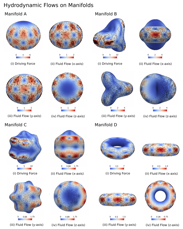
Figure 4: Surface Hydrodynamic Flows on Manifolds $A$–$D$. We use our GMLS solver to compute numerically the surface hydrodynamic flow responses on each of the manifolds, as discussed in Section 4.2. Manifold $A-D$ solutions were computed at a resolution with number of sample points $n_{A}=38,486,n_{B}=147,634,n_{C}=127,346,$ and $n_{D}=118,942$.

We investigate the convergence of our GMLS methods for the surface hydrodynamic equations formulated in Section 4. We study convergence of our solvers for hydrodynamic flows by developing manufactured solutions using high precision symbolic calculations of the incompressible flow field $\mathbf{v}^{\flat}=-\star\mathbf{d}\Phi=\mathcal{C}_{0}\Phi$ with the specific choice of $\Phi$ given in Section 6.1.

We calculate symbolically the expressions of the forcing term $\mathbf{b}$ using equation 22 where $\mu_{m}(-\bm{\delta}\mathbf{d}+2K)\mathbf{v}^{\flat}-\gamma\mathbf{v}^{\flat}-\mathbf{d}p=-\mathbf{b}^{\flat}$. We manufacture the data $\mathbf{b}$ needed on the RHS of equation 22 using

$$\mathbf{b}^{\flat}=\mu_{m}\bm{\delta}\mathbf{d}\mathbf{v}^{\flat}+(\gamma-2\mu_{m}K)\mathbf{v}^{\flat}.$$ (31)

Since generating both the velocity field $\mathbf{v}$ and force density $\mathbf{b}$ this way will already be incompressible, we have used that we can set $p=0$ when manufacturing our data. In practice, we evaluate equation 31 to high precision using the symbolic package SymPy [68].

We investigate the convergence of the GMLS solvers using the $\ell^{2}$-error

$$\epsilon_{hydro} = \left\|\tilde{\mathbf{v}}-\mathbf{v}\right\|_{2}/\|\mathbf{v}\|_{2}$$ (32)

$$\tilde{\mathbf{v}} = \mathcal{C}_{0}(\mathcal{S}^{-1}(\mathcal{C}_{0}\mathbf{b})).$$ (33)

The $\mathbf{v}$ denotes the exact solution, $\mathcal{C}_{0}$ approximates numerically $-\star\mathbf{d}_{0}$, $\mathcal{C}_{1}$ approximates numerically $-\star\mathbf{d}_{1}$, and $\mathcal{S}^{-1}$ denotes the numerical solution operator corresponding to use of our GMLS solver. We use the hydrodynamics equations both formulated using the biharmonic form in equation 26 or in the split form in equation 27.

For each of the manifolds $A-D$, we computed manufactured solutions with the parameters $\mu_{m}=0.1$, $\gamma=0.1$ in equation 31. We used the surface force density $\mathbf{b}$ to numerically compute surface hydrodynamic flow responses $\tilde{\mathbf{v}}$ using our GMLS solvers discussed in Section 5. We show the hydrodynamic surface flows in Figure 4. We show our convergence results for both the case of the biharmonic formulation and split formulation in the Tables 5– 8.

Biharmonic Formulation: Manifold A

	m = 4		m = 6		m = 8
h	$\ell_{2}$-error	Rate	$\ell_{2}$-error	Rate	$\ell_{2}$-error	Rate
0.1	1.6072e-01	-	1.1597e-03	-	1.0648e-03	-
0.05	1.8027e-02	3.11	8.4190e-05	3.73	1.8627e-06	9.04
0.025	4.9155e-03	1.86	1.1655e-05	2.84	4.4796e-08	5.35
0.0125	2.0873e-03	1.23	7.1161e-07	4.02	1.9263e-07	-2.10

Split Formulation: Manifold A

	m = 4		m = 6		m = 8
h	$\ell_{2}$-error	Rate	$\ell_{2}$-error	Rate	$\ell_{2}$-error	Rate
0.1	1.5578e-02	-	2.6826e-04	-	1.0756e-04	-
0.05	7.0783e-04	4.40	1.2065e-05	4.41	3.7309e-07	8.06
0.025	1.2151e-05	5.83	4.4532e-07	4.74	3.0556e-09	6.90
0.0125	4.3056e-06	1.49	1.0349e-08	5.42	1.7664e-10	4.10

Table 5: (top) Convergence on Manifold A of our GMLS solver based on the biharmonic formulation of the hydrodynamics in equation 26. The target sampling distance $h$ is discussed in Appendix D. (bottom) Convergence on Manifold A of our GMLS solver based on the split formulation of the hydrodynamics in equation 27.

Biharmonic Formulation: Manifold B

	m = 4		m = 6		m = 8
h	$\ell_{2}$-error	Rate	$\ell_{2}$-error	Rate	$\ell_{2}$-error	Rate
0.1	3.1890e-01	-	1.0457e-01	-	1.6845e+00	-
0.05	3.1951e-01	-0.002	7.4388e-03	3.81	1.9954e-02	6.40
0.025	2.4571e-02	3.69	1.2081e-03	2.62	2.9917e-04	6.05
0.0125	5.6309e-03	2.12	6.9269e-05	4.11	2.6601e-05	3.48

Split Formulation: Manifold B

	m = 4		m = 6		m = 8
h	$\ell_{2}$-error	Rate	$\ell_{2}$-error	Rate	$\ell_{2}$-error	Rate
0.1	9.7895e-02	-	6.5222e-02	-	2.8024e-01	-
0.05	1.4383e-02	2.77	2.8402e-03	4.52	1.2100e-02	4.53
0.025	3.6243e-03	1.98	3.9929e-04	2.82	4.9907e-04	4.59
0.0125	7.8747e-04	2.20	1.2357e-05	5.00	5.7023e-06	6.44

Table 6: (top) Convergence on Manifold B of our GMLS solver based on the biharmonic formulation of the hydrodynamics in equation 26. (bottom) Convergence on Manifold B of our GMLS solver based on the split formulation of the hydrodynamics in equation 27.

Biharmonic Formulation: Manifold C

	m = 4		m = 6		m = 8
h	$\ell_{2}$-error	Rate	$\ell_{2}$-error	Rate	$\ell_{2}$-error	Rate
0.1	2.9886e+00	-	8.0650e-01	-	3.3799e-01	-
0.05	1.2926e+00	1.21	2.3277e-01	1.79	1.0993e+00	-1.70
0.025	2.8576e-01	2.18	2.1497e-02	3.44	7.1166e-03	7.28
0.0125	4.2226e-02	2.76	1.4986e-03	3.84	9.8921e-05	6.17

Split Formulation: Manifold C

	m = 4		m = 6		m = 8
h	$\ell_{2}$-error	Rate	$\ell_{2}$-error	Rate	$\ell_{2}$-error	Rate
0.1	1.1346e+00	-	8.8130e+01	-	4.6473e+00	-
0.05	7.7801e-02	3.86	1.0276e-02	13.0	3.7375e-02	6.96
0.025	1.6751e-02	2.22	1.8764e-03	2.45	4.2722e-04	6.46
0.0125	1.7381e-03	3.27	4.2181e-05	5.48	9.1845e-06	5.54

Table 7: (top) Convergence on Manifold C of our GMLS solver based on the biharmonic formulation of the hydrodynamics in equation 26. (bottom) Convergence on Manifold C of our GMLS solver based on the split formulation of the hydrodynamics in equation 27.

Biharmonic Formulation: Manifold D

	m = 4		m = 6		m = 8
h	$\ell_{2}$-error	Rate	$\ell_{2}$-error	Rate	$\ell_{2}$-error	Rate
0.08	3.3170e-01	-	1.5154e-01	-	1.2223e+01	-
0.04	2.4421e-02	3.82	4.6233e-03	5.11	3.9632e-03	11.7
0.02	4.5705e-03	2.44	3.0246e-04	3.97	4.2784e-05	6.60
0.01	1.4748e-03	1.62	1.9067e-05	3.96	5.4137e-07	6.26

Split Formulation: Manifold D

	m = 4		m = 6		m = 8
h	$\ell_{2}$-error	Rate	$\ell_{2}$-error	Rate	$\ell_{2}$-error	Rate
0.08	1.7719e-02	-	1.4221e-02	-	6.6061e+00	-
0.04	1.5473e-03	3.57	1.2632e-04	6.92	1.3431e-04	15.8
0.02	1.3575e-04	3.54	3.2125e-06	5.35	5.0041e-07	8.15
0.01	2.5891e-05	2.37	1.9018e-07	4.05	4.5906e-09	6.72

Table 8: (top) Convergence on Manifold D of our GMLS solver based on the biharmonic formulation of the hydrodynamics in equation 26. (bottom) Convergence on Manifold D of our GMLS solver based on the split formulation of the hydrodynamics in equation 27.

We emphasize that these convergence studies take into account the full pipeline of our GMLS numerical methods as discussed in Section 5 and shown in Figure 3. This involves not only the solution of biharmonic or split equations, but also the GMLS reconstruction of the surface velocity field $\mathbf{v}$ from the computed vector-potential $\Phi$ and the calculation of the vector-potentials $\Psi=-\star\mathbf{d}\mathbf{b}$ for the body force density $\mathbf{b}$ which drives the flow. These steps also each have a non-linear dependence on the geometry which contributes through our GMLS reconstructions from the point set sampling of the manifold as discussed in Section 3.

In the convergence studies, we find in all cases that the GMLS solvers are able to resolve the surface hydrodynamic fields to a high level of precision. The Manifolds $B$ and $C$ presented the most challenges for the solvers with largest prefactors in their convergence. This is expected given the increased amount of resolution required to resolve the geometric contributions to the differential operators in the hydrodynamic equations 26– 27. In all cases, we found our GMLS solvers based on the split formulation performed better when using equation 27 relative to our GMLS solvers based on the biharmonic formulation of equation 26. Interestingly, for Manifold $B$ and $C$ these differences for $m=8$ where not as pronounced, see Table 6– 7. We think this is a manifestation of the challenges in capturing the geometric contributions to the differential operator that with limited resolution will not benefit as much from the higher order approximations or split formulations relative to the case of less complicated geometries.

We find in the case of Manifold $A$ that the GMLS solver for sufficiently large order ($m\geq 6$) converges at a rate of approximately $\sim 4^{th}$-order for the biharmonic formulation and at a rate of approximately $\sim 5^{th}$-order for the split formulation. We base this on the overall trends, and some of this is a little obscured by the noise of the convergence after acheiving a high level of accuracy. We suspect the last upward point of the error observed for $m=8$ for the biharmonic formulation is likely a consequence of the conditioning of the linear system becoming a limiting factor. We note the overall high level of precision already achieved by that data point with errors on the order of $10^{-8}$, see Table 5. We find there is a particular advantage of our GMLS solvers when based on the split formulation. Our GMLS methods in this case are able to converge to much higher levels of precision achieving errors on the order $10^{-10}$ in the case of $m=8$ at the largest resolutions considered, see Table 5.

In summary, our results show that both formulations of the GMLS solvers are able to achieve high-order convergence rates in approximating the hydrodynamic fields. We emphasize that these results assess contributions from the entire pipeline that includes not only the GMLS solve but also the pre-processing and post-processing steps involving the curl operators that arise in our vector-potential formulation for incompressible hydrodynamic flows.

7 Conclusions

We have developed high-order numerical methods for solving partial differential equations on manifolds. Our apporach is based on GMLS approximations of the manifold shape, operators arising in differential geometry, and operators of differential equations. We have introduced exterior calculus based approaches for generalizing the operators of vector calculus and techniques from mechanics to the context of manifolds. Using this approach, we have formulated incompressible hydrodynamic equations for flows on curved surfaces. We have also shown how our approaches in general can be used to formulate equations in terms of vector potentials facilitating development of other physical models with constraints to obtain numerical solvers. We showed there are a few different ways to formulate vector-valued surface equations facilitating the development of GMLS solvers. By comparisons with high precision manufactured solutions, we characterized our GMLS solvers and found they each exhibit high-order convergence rates in approximating manifold operators and in resolving hydrodynamics flows on surfaces. We found the split formulations involving lower order differential operators to have particular advantages exhibiting the highest orders of convergence. Many of our GMLS methods and exterior calculus approaches also can be utilized for the development of high-order solvers for other scalar-valued and vector-valued partial differential equations on manifolds.

Appendix

Appendix A Operators on Manifolds, Monge-Gauge Parameterization, and Coordinate Expressions

To compute in practice the action of our operators during the GMLS reconstruction of the geometry of the manifolds or differential operators on scalar and vector fields on the surface, we use local Monge-Gauge parameterizations of the surface. To obtain high-order accuracy we further expand expressions involving derivatives of the metric and other fields explicitly using symbolic algebra packages, such as Sympy [68]. This allows us to avoid some of the tedium notorous in differential geometry and to precompute offline the needed expressions for the action of our operators. We summarize here the basic differential geometry of surfaces expressed in the Monge-Gauge and the associated expressions we use in such calculations.

A.1 Monge-Gauge Surface Parameterization

In the Monge-Gauge we parameterize locally a smooth surface in terms of the tangent plane coordinates $u,v$ and the height of the surface above this point as the function $h(u,v)$. This gives the embedding map

$$\mathbf{x}(u,v)=\bm{\sigma}(u,v)=(u,v,\mathbf{h}(u,v)).$$ (34)

We see that this parameterization of the surface is closely related to equation 8. We can use the Monge-Gauge equation 34 to derive explicit expressions for geometric quantities. The derivatives of $\bm{\sigma}$ provide a basis $\partial_{u},\partial_{v}$ for the tangent space as

$$\partial_{u}=\bm{\sigma}_{u}(u,v) = (1,0,\mathbf{h}_{u}(u,v))$$ (35)

$$\partial_{v}=\bm{\sigma}_{v}(u,v) = (0,1,\mathbf{h}_{v}(u,v)).$$ (36)

The first fundamental form $\mathbf{I}$ (metric tensor) and second fundamental form $\mathbf{II}$ (curvature tensor) are given by

$$\mathbf{I}=\begin{bmatrix}E&F\\ F&G\end{bmatrix}=\begin{bmatrix}\bm{\sigma}_{u}\cdot\bm{\sigma}_{u}&\bm{\sigma}_{u}\cdot\bm{\sigma}_{v}\\ \bm{\sigma}_{v}\cdot\bm{\sigma}_{u}&\bm{\sigma}_{v}\cdot\bm{\sigma}_{v}\end{bmatrix}=\begin{bmatrix}1+\mathbf{h}_{u}(u,v)^{2}&\mathbf{h}_{u}\mathbf{h}_{v}(u,v)\\ \mathbf{h}_{u}(u,v)\mathbf{h}_{v}(u,v)&1+\mathbf{h}_{v}(u,v)^{2}\end{bmatrix}.$$ (37)

and

$$\mathbf{II}=\begin{bmatrix}L&M\\ M&N\end{bmatrix}=\begin{bmatrix}\bm{\sigma}_{uu}\cdot\bm{n}&\bm{\sigma}_{uv}\cdot\bm{n}\\ \bm{\sigma}_{vu}\cdot\bm{n}&\bm{\sigma}_{vv}\cdot\bm{n}\end{bmatrix}=\frac{1}{\sqrt{1+\mathbf{h}_{u}^{2}+\mathbf{h}_{v}^{2}}}\begin{bmatrix}\mathbf{h}_{uu}&\mathbf{h}_{uv}\\ \mathbf{h}_{uv}&\mathbf{h}_{vv}\end{bmatrix}.$$ (38)

The $\mathbf{n}$ denotes the outward normal on the surface and is given by

$$\bm{n}(u,v)=\frac{\bm{\sigma}_{u}(u,v)\times\bm{\sigma}_{v}(u,v)}{\|\bm{\sigma}_{u}(u,v)\times\bm{\sigma}_{v}(u,v)\|}=\frac{1}{\sqrt{1+\mathbf{h}_{u}^{2}+\mathbf{h}_{v}^{2}}}(-\mathbf{h}_{u},-\mathbf{h}_{v},1).$$ (39)

We use throughout the notation for the metric tensor $\mathbf{g}=\mathbf{I}$ interchangeably. For notational convenience, we use the tensor notation for the metric tensor $g_{ij}$ and for its inverse $g^{ij}$. These correspond to the first and second fundamental forms as

$$g_{ij}=\left[\mathbf{I}\right]_{i,j},\hskip 8.5359ptg^{ij}=\left[\mathbf{I}^{-1}\right]_{i,j}.$$ (40)

For the metric tensor $\mathbf{g}$, we also use the notation $|g|=\det(\mathbf{g})$ and have that

$$\sqrt{|g|}=\sqrt{\det(\mathbf{I})}=\sqrt{1+\mathbf{h}_{u}^{2}+\mathbf{h}_{v}^{2}}=\|\vec{\sigma}_{u}(u,v)\times\vec{\sigma}_{v}(u,v)\|.$$ (41)

The provides the local area element as $dA_{u,v}=\sqrt{|g|}dudv$. To compute quantities associated with curvature of the manifold we construct the Weingarten map [85] which can be expressed as

$$\mathbf{W}=\mathbf{I}^{-1}\mathbf{II}.$$ (42)

The Gaussian curvature $K$ can be expressed in the Monge-Gauge as

$$K(u,v)=\det\left(\mathbf{W}(u,v)\right)=\frac{\mathbf{h}_{uu}\mathbf{h}_{vv}-\mathbf{h}_{uv}^{2}}{(1+\mathbf{h}_{u}^{2}+\mathbf{h}_{v}^{2})^{2}}.$$ (43)

For further discussions of these tensors and more generally the differential geometry of manifolds see [85, 1, 101]. We use these expressions as the basis of our calculations of the action of our surface operators.

A.2 Coordinate Expressions for Surface Operators

We use local Monge-Gauge parameterizations of the manifold to compute the geometric operators needed in our surface hydrodynamic equations. Consider the negative semi-definite scalar Laplace-Beltrami operator that acts on $0$-forms which can be expressed as $\Delta_{LB}=-\bm{\delta}\mathbf{d}=-\Delta_{H}$, where $\Delta_{H}$ is the Hodge Laplacian. This operator can be expressed in coordinates as

$$\Delta_{LB}=\frac{1}{\sqrt{|g|}}\partial_{i}\left(g^{ij}\sqrt{|g|}\partial_{j}\right).$$ (44)

The $g_{ij}$ denotes the metric tensor, $g^{ij}$ the inverse metric tensor, and $|g|$ the determinant of the metric tensor as in Appendix A.1. For the Monge-Gauge parameterization $(u,v)$, we find it useful to consider

$$\ell_{ij}=\left(\sqrt{|g|}g^{ij}\right)\partial_{ij}+\left(\partial_{i}\sqrt{|g|}g^{ij}\right)\partial_{j}.$$ (45)

We use the convention that $\partial_{1}=\partial_{u}$ and $\partial_{2}=\partial_{v}$. This allows us to express

$$\Delta_{LB}=(1/\sqrt{|g|})\sum_{ij}\ell_{ij}.$$ (46)

We can further express the prefactor terms involving the metric appearing in equation 45 as

$$\sqrt{|g|}g^{ij}=\begin{cases}{g_{vv}}/{\sqrt{|g|}}=\frac{1+\mathbf{h}_{v}^{2}}{\sqrt{1+\mathbf{h}_{u}^{2}+\mathbf{h}_{v}^{2}}}&\text{if: $i=j=u$}\\ {g_{uu}}/{\sqrt{|g|}}=\frac{1+\mathbf{h}_{u}^{2}}{\sqrt{1+\mathbf{h}_{u}^{2}+\mathbf{h}_{v}^{2}}}&\text{if: $i=j=v$}\\ {-g_{uv}}/{\sqrt{|g|}}={-g_{vu}}/{\sqrt{|g|}}=\frac{-\mathbf{h}_{u}\mathbf{h}_{v}}{\sqrt{1+\mathbf{h}_{u}^{2}+\mathbf{h}_{v}^{2}}}&\text{if: $i\neq j$}.\end{cases}$$ (47)

The utility of these decompositions and expressions is that we can construct operators for GMLS approximation while avoiding the need to compose numerical differentiation procedures. This allows us to compute directly the action on the reconstruction space functions $p\in\mathbb{V}_{h}$. This decomposition is also useful to help simplify symbolic expansions when we compute the Bi-Laplace-Beltrami operator $\Delta_{LB}^{2}$, which poses the most significant computational challenges in our current numerical calculations. We compute in practice the Bi-Laplace-Beltrami operator $\Delta_{LB}^{2}$ using symbolic algebra system.

A.3 Exterior Calculus Operators Expressed in Coordinates

In our notations throughout, we take the conventions that for differential $0$-forms (scalar functions) $f_{j}=\partial_{x^{j}}f$, for differential $1$-forms (co-vector fields) $\bm{\alpha}=\alpha_{j}\mathbf{d}{x}^{j}$, and for vector fields $\mathbf{v}=v^{j}\partial_{j}$. In each case we have $j\in\{u,v\}$. The isomorphisms $\sharp$ and $\flat$ between vectors and co-vectors can be expressed explicitly as

$$\mathbf{v}^{\flat} = (v^{u}\bm{\sigma}_{u}+v^{v}\bm{\sigma}_{v})^{\flat}$$

$$= v^{u}g_{uu}\mathbf{d}u+v^{u}g_{uv}\mathbf{d}v+v^{v}g_{vu}\mathbf{d}u+v^{v}g_{vv}\mathbf{d}v$$

$$= (v^{u}g_{uu}+v^{v}g_{vu})\mathbf{d}u+(v^{u}g_{uv}+v^{v}g_{vv})\mathbf{d}v$$

$$(\bm{\alpha})^{\sharp} = (\alpha_{u}\mathbf{d}u+\alpha_{v}\mathbf{d}v)^{\sharp}$$

$$= \alpha_{u}g^{uu}\bm{\sigma}_{u}+\alpha_{u}g^{uv}\bm{\sigma}_{v}+\alpha_{v}g^{vu}\bm{\sigma}_{u}+\alpha_{v}g^{vv}\bm{\sigma}_{v}$$

$$= (\alpha_{u}g^{uu}+\alpha_{v}g^{vu})\bm{\sigma}_{u}+(\alpha_{u}g^{uv}+\alpha_{v}g^{vv})\bm{\sigma}_{v}$$

We use the conventions for the notation that for the embedding map $\bm{\sigma}$ we have $\bm{\sigma}_{u}=\partial_{u}$ and $\bm{\sigma}_{v}=\partial_{v}$ as in Appendix A.1. The exterior derivatives on these $k$-forms can be expressed as

$$\mathbf{d}f = (\partial_{u}f)\mathbf{d}u+(\partial_{v}f)\mathbf{d}v=f_{u}\mathbf{d}u+f_{v}\mathbf{d}v$$ (50)

$$\mathbf{d}\bm{\alpha} = (\partial_{u}\alpha_{v}-\partial_{v}\alpha_{u})\mathbf{d}u\wedge\mathbf{d}v.$$ (51)

The generalized curl of a $0$-form and $1$-form can be expressed in coordinates as

$$-\star\mathbf{d}f = \sqrt{|g|}(f_{u}g^{uv}+f_{v}g^{vv})\mathbf{d}u-\sqrt{|g|}(f_{u}g^{uu}+f_{v}g^{vu})\mathbf{d}v$$ (52)

$$-\star\mathbf{d}\alpha = \frac{\partial_{v}\alpha_{u}-\partial_{u}\alpha_{v}}{\sqrt{|g|}}.$$ (53)

Combining the above equations, we can express the generalized curl as

$$(-\star\mathbf{d}f)^{\sharp} = \mbox{curl}_{\mathcal{M}}(f)$$

$$= ([\sqrt{|g|}(f_{u}g^{uv}+f_{v}g^{vv})]g^{uu}+[-\sqrt{|g|}(f_{u}g^{uu}+f_{v}g^{vu})]g^{vu})\bm{\sigma}_{u}$$

$$+ ([\sqrt{|g|}(f_{u}g^{uv}+f_{v}g^{vv})]g^{uv}+[-\sqrt{|g|}(f_{u}g^{uu}+f_{v}g^{vu})]g^{vv})\bm{\sigma}_{v}$$

$$= \frac{f_{v}}{\sqrt{|g|}}\bm{\sigma}_{u}-\frac{f_{u}}{\sqrt{|g|}}\bm{\sigma}_{v}$$

$$-\star\mathbf{d}\mathbf{v}^{\flat} = \mbox{curl}_{\mathcal{M}}(\mathbf{v})=\frac{\partial_{v}(v^{u}g_{uu}+v^{v}g_{vu})-\partial_{u}(v^{u}g_{uv}+v^{v}g_{vv})}{\sqrt{|g|}}.$$ (55)

We also mention that the velocity field of the hydrodynamic flows $\mathbf{v}$ is recovered from the vector potential $\Phi$ as $\mathbf{v}^{\flat}=-\star\mathbf{d}\Phi$. We obtain the velocity field as $\mathbf{v}=\left(\mathbf{v}^{\flat}\right)^{\sharp}=\left(-\star\mathbf{d}\Phi\right)^{\sharp}$ using equation A.3. Similarly from the force density $\mathbf{b}$ acting on the fluid, we obtain from equation 55 the vector potential for the force density as $\Psi=-\star\mathbf{d}\mathbf{b}^{\flat}$. This is used in the vector-potential formulation of the hydrodynamics in equation 26 and equation 27. We expand these expressions further as needed in coordinates using symbolic algebra methods. This provides the needed expressions for computing these operations. Additional details and discussions of these operators and our overall approach also can be found in our related papers [99, 44].

Appendix B Convergence Results for the Generalized Curl Operators

We report tabulated results for the GMLS approximations of the operators $\mathcal{L}_{C0}$ and $\mathcal{L}_{C1}$ discussed in Section 6.1.

	Manifold A		Manifold B		Manifold C				Manifold D
h	$\ell_{2}$-error	Rate	$\ell_{2}$-error	Rate	$\ell_{2}$-error	Rate		h	$\ell_{2}$-error	Rate
0.1	2.7152e-05	-	1.5075e-03	-	4.8243e-01	-		.08	2.1570e-03	-
0.05	3.8309e-07	6.07	3.0281e-05	5.64	2.4465e-04	10.9		.04	2.2565e-05	6.68
0.025	5.8491e-09	6.00	6.9649e-07	5.43	6.1779e-06	5.31		.02	3.3550e-07	6.13
0.0125	8.8291e-11	6.04	1.3078e-08	5.72	1.1817e-07	5.71		.01	4.9708e-09	6.04

Table 9: Convergence of GMLS Approximation of the Surface Curl Operator on Scalars $\mathcal{L}_{C0}$. We use GMLS with ($k=1,m=6)$ and find the methods have $\sim 6^{th}$-order asymptotic convergence.

	Manifold A		Manifold B		Manifold C				Manifold D
h	$\ell_{2}$-error	Rate	$\ell_{2}$-error	Rate	$\ell_{2}$-error	Rate		h	$\ell_{2}$-error	Rate
0.1	9.2312e-04	-	1.5887e-02	-	5.2497e+01	-		.08	1.9686e-02	-
0.05	1.4851e-05	5.88	1.2736e-03	3.64	1.3126e-02	8.65		.04	2.0410e-04	6.70
0.025	2.3374e-07	5.96	1.2597e-04	3.33	5.6087e-04	4.55		.02	3.0223e-06	6.13
0.0125	3.5970e-09	6.01	5.1267e-06	4.61	1.4082e-05	5.32		.01	4.3847e-08	6.07

Table 10: Convergence of GMLS Approximation of the Surface Curl Operator on Vectors $\mathcal{L}_{C1}$. We use GMLS with ($k_{1}=2,k_{2}=1,m=6)$ and find the methods have $\sim 5^{th}$-order asymptotic convergence or greater. It is notable that in the case of Manifold $A$ and $D$ we in fact see $\sim 6^{th}$-order convergence. This manifests since the manifolds have a relatively symmetric geometry compared to Manifold $B$ and $C$, see Figure 2. This results in a simplification with fewer non-zero terms and derivatives associated with the contributions of the geometry to the operator. As a consequence, the GMLS approximation at a given order $m$ becomes more accurate by one order for Manifold $A$ and $D$.

The Manifolds B and C have more complicated geometry and require more resolution to see behaviors in the asymptotic regime with a high-degree basis. We see that by lowering the degree of the basis these operators exhibit more readily behaviors in the asymptotic regime in Table 11 and 12.

	Manifold B		Manifold C
h	$\ell_{2}$-error	Rate	$\ell_{2}$-error	Rate
0.1	5.2558e-03	-	1.2083e-02	-
0.05	3.6359e-04	3.85	1.0345e-03	3.54
0.025	2.3078e-05	3.97	7.3790e-05	3.81
0.0125	1.4569e-06	3.98	4.8316e-06	3.93

Table 11: Convergence of GMLS Approximation of the Surface Curl on Scalars $\mathcal{L}_{C0}$. We use GMLS with ($k=1,m=4)$ and find the methods have $\sim 4^{th}$-order asymptotic convergence.

	Manifold B		Manifold C
h	$\ell_{2}$-error	Rate	$\ell_{2}$-error	Rate
0.1	6.3586e-01	-	7.6579e-01	-
0.05	1.6568e-01	1.94	2.1680e-01	1.82
0.025	4.1633e-02	1.99	5.6498e-02	1.94
0.0125	1.0399e-02	1.99	1.4336e-02	1.98

Table 12: Convergence of GMLS Approximation of the Surface Curl on Vectors $\mathcal{L}_{C1}$. We use GMLS with ($k=1,m=2)$ and find the methods have $\sim 2^{nd}$-order asymptotic convergence.

Appendix C Dependence of GMLS Approximations on the Point Sampling

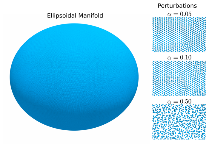
Figure 5: Ellipsoidal Manifold, Point Samples, and Perturbations. (left) The ellipsoidal manifold with $(x/\ell_{x})^{2}+(y/\ell_{y})^{2}+(z/\ell_{z})^{2}=1$ with $\ell_{x}=1.2$, $\ell_{y}=1.2$, $\ell_{z}=1$. The manifold is sampled with $154,182$ points. (right) The points are perturbed by noise having strength $\alpha=0.05,0.10,0.50$.

We investigate the dependence of the GMLS approximations on the point sampling. We perform studies of the sampling of the manifold perturbed by noise. As discussed in Appendix D, we start with the manifold sampled by a collection of points $\{x_{i}\}$ using DistMesh [80]. These are nearly uniform as characterized by equation 1. We then add Gaussian noise $\eta_{i}$ with mean zero and standard derivation of $\sigma=\alpha\ell_{*}$ to each of the points $x_{i}$. The $\ell_{*}$ is $1/3$ the smallest nearest neighbor distance. We project these points back to the manifold to obtain the new perturbed sampling $\tilde{x}_{i}=\mathcal{P}(x_{i}+\eta_{i})$, where $\mathcal{P}$ denotes the projection mapping. For the radial manifold shapes, $\mathcal{P}$ is the mapping back to the manifold along the radial directions. We study the perturbations when $\alpha\in\{0.05,0.1,0.5\}$ for the ellipsoid $(x/\ell_{x})^{2}+(y/\ell_{y})^{2}+(z/\ell_{z})^{2}=1$ with $\ell_{x}=1.2$, $\ell_{y}=1.2$, $\ell_{z}=1$. We show realizations of the point sampling and perturbations in Figure 5 and the results of our convergence studies in Table 13.

	Laplace-Beltrami		Biharmonic
$\alpha$	$\ell_{2}$-error	Rate	$\ell_{2}$-error	Rate
0.00	3.437-04	2.03	2.828-04	2.54
0.05	3.425-04	2.03	8.655-04	2.20
0.10	3.419-04	2.04	9.032-04	2.17
0.50	3.650-04	2.07	1.464-03	2.18

Table 13: Dependence of GMLS Approximations on the Point Sampling. We investigate the convergence when perturbing the manifold sample points by $\tilde{x}_{i}=\mathcal{P}(x_{i}+\eta_{i})$ where the Gaussian noise $\eta_{i}$ has mean zero and standard deviation of $\sigma=\alpha\ell_{*}$. The $\ell_{*}$ is $1/3$ of the smallest nearest neighbor distance for the unperturbed sampling. We consider the ellipsoidal manifold with $(x/\ell_{x})^{2}+(y/\ell_{y})^{2}+(z/\ell_{z})^{2}=1$ with $\ell_{x}=1.2$, $\ell_{y}=1.2$, $\ell_{z}=1$ sampled with the number of sample points $2,350$, $9,566$, $38,486$, and $154,182$. We study the accuracy of the solvers for $\mathcal{L}u=-f$ where $\mathcal{L}$ is the Laplace-Beltrami Operator and the Biharmonic Operator. The solver for the Biharmonic Operator uses the split formulation. The function $f$ is generated using angular coordinates to obtain the real-part of the spherical harmonic $Y_{4}^{5}$ projected to the ellipsoidal surface. The ellipsoid considered is given by $(x/\ell_{x})^{2}+(y/\ell_{y})^{2}+(z/\ell_{z})^{2}=1$ with $\ell_{x}=1.2$, $\ell_{y}=1.2$, $\ell_{z}=1$.

From Table 13, we see that the GMLS methods are robust to perturbations in the sampling both for the Laplace-Beltrami Operator and for the Biharmonic Operator. We remark that these solvers each have a non-trivial dependence not only on the approximation of the differential operators but also in the approximations performed for the local geometry of the manifold. This indicates in GMLS that the local least-squares fitting is not overly sensitive to the point sampling that is used in constructing the approximations.

Appendix D Sampling Resolution of the Manifolds

A summary of the sampling resolution $h$ used for each of the manifolds is provided in Table 14. We refer to $h$ as the target fill distance. For each of the manifolds, we achieve a nearly uniform collection of the points as in equation 1 using DistMesh [80]. We emphasize this approach was used only for convenience to obtain quasi-uniform samplings and other sampling techniques can also be utilized for this purpose of representing the manifolds. We specify $h$ and the algorithm produces a point sampling of the manifold. In practice, we have found this yields a point spacing with neighbor distances varying by only $\approx\pm 30\%$ relative to the target distance $h$. We summarize for each of the manifolds how this relates to the number of sample points $n$ in Table 14.

Refinement Level	A: h	n	B: h	n	C: h	n	D: h	n
$1$	.1	2350	.1	2306	.1	2002	.08	1912
$2$	.05	9566	.05	9206	.05	7998	.04	7478
$3$	.025	38486	.025	36854	.025	31898	.02	29494
$4$	.0125	154182	.0125	147634	.0125	127346	.01	118942

Table 14: Sampling Resolution for each of the Manifolds A–D. Relation between the target distance $h$ and the number of sample points $n$ used for each of the manifolds. In each case, the neighbor distances between the points sampled were within $\approx\pm 30\%$ of the target distance $h$.

References

- [1] R. Abraham, J.E. Marsden, and T.S. Ratiu. Manifolds, Tensor Analysis, and Applications. Number v. 75. Springer New York, 1988.
- [2] D. J. Acheson. Elementary Fluid Dynamics. Oxford Applied Mathematics and Computing Science Series, 1990.
- [3] D. J. Acheson. Elementary Fluid Dynamics. Oxford Applied Mathematics and Computing Science Series, 1990.
- [4] Clarisse Alboin, Jérôme Jaffré, Jean E Roberts, and Christophe Serres. Modeling fractures as interfaces for flow and transport. Fluid Flow and Transport in Porous Media, Mathematical and Numerical Treatment, 295:13, 2002.
- [5] Marino Arroyo Alejandro Torres-Sanchez, Daniel Santos-Oliván. Approximation of tensor fields on surfaces of arbitrary topology based on local monge parametrizations. arXiv, 2019.
- [6] P. Alliez, D. Cohen-Steiner, Y. Tong, and M. Desbrun. Voronoi-based variational reconstruction of unoriented point sets. In Proceedings of the Fifth Eurographics Symposium on Geometry Processing, SGP ’07, pages 39–48, Aire-la-Ville, Switzerland, Switzerland, 2007. Eurographics Association.
- [7] Nina Amenta and Yong Joo Kil. Defining point-set surfaces. In ACM SIGGRAPH 2004 Papers, SIGGRAPH ’04, pages 264–270, New York, NY, USA, 2004. ACM.
- [8] Douglas N Arnold, Pavel B Bochev, Richard B Lehoucq, Roy A Nicolaides, and Mikhail Shashkov. Compatible spatial discretizations, volume 142. Springer Science & Business Media, 2007.
- [9] Douglas N. Arnold, Richard S. Falk, and Ragnar Winther. Finite element exterior calculus, homological techniques, and applications. Acta Numerica, 15:1–155–, 2006.
- [10] Marino Arroyo and Antonio DeSimone. Relaxation dynamics of fluid membranes. Phys. Rev. E, 79(3):031915–, March 2009.
- [11] John W Barrett, Harald Garcke, and Robert Nürnberg. A parametric finite element method for fourth order geometric evolution equations. Journal of Computational Physics, 222(1):441–467, 2007.
- [12] G. K. Batchelor. An Introduction to Fluid Dynamics. Cambridge Mathematical Library. Cambridge University Press, 2000.
- [13] Eric Bavier, Mark Hoemmen, Sivasankaran Rajamanickam, and Heidi Thornquist. Amesos2 and belos: Direct and iterative solvers for large sparse linear systems. Scientific Programming, 20(3), 2012.
- [14] Marcelo Bertalmío, Facundo Mémoli, Li-Tien Cheng, Guillermo Sapiro, and Stanley Osher. Variational Problems and Partial Differential Equations on Implicit Surfaces: Bye Bye Triangulated Surfaces?, pages 381–397. Springer New York, New York, NY, 2003.
- [15] Pavel B. Bochev and James M. Hyman. Principles of mimetic discretizations of differential operators. In Douglas N. Arnold, Pavel B. Bochev, Richard B. Lehoucq, Roy A. Nicolaides, and Mikhail Shashkov, editors, Compatible Spatial Discretizations, pages 89–119, New York, NY, 2006. Springer New York.
- [16] R. J. Braun, R. Usha, G. B. McFadden, T. A. Driscoll, L. P. Cook, and P. E. King-Smith. Thin film dynamics on a prolate spheroid with application to the cornea. Journal of Engineering Mathematics, 73(1):121–138, Apr 2012.
- [17] Susanne Brenner and Ridgway Scott. The Mathematical Theory of Finite Element Methods. Springer, 2008.
- [18] Martin D Buhmann. Radial basis functions: theory and implementations, volume 12. Cambridge university press, 2003.
- [19] Marcello Cavallaro, Lorenzo Botto, Eric P. Lewandowski, Marisa Wang, and Kathleen J. Stebe. Curvature-driven capillary migration and assembly of rod-like particles. Proceedings of the National Academy of Sciences, 108(52):20923–20928, 2011.
- [20] Alexey Y Chernyshenko and Maxim A Olshanskii. An unfitted finite element method for the darcy problem in a fracture network. arXiv preprint arXiv:1903.06351, 2019.
- [21] Keenan Crane, Fernando de Goes, Mathieu Desbrun, and Peter Schröder. Digital geometry processing with discrete exterior calculus. In ACM SIGGRAPH 2013 Courses, SIGGRAPH ’13, pages 7:1–7:126, New York, NY, USA, 2013. ACM.
- [22] M. Desbrun, A. N. Hirani, and J. E. Marsden. Discrete exterior calculus for variational problems in computer vision and graphics. In 42nd IEEE International Conference on Decision and Control (IEEE Cat. No.03CH37475), volume 5, pages 4902–4907 Vol.5, 2003.
- [23] Yegor A. Domanov, Sophie Aimon, Gilman E. S. Toombes, Marianne Renner, François Quemeneur, Antoine Triller, Matthew S. Turner, and Patricia Bassereau. Mobility in geometrically confined membranes. Proceedings of the National Academy of Sciences, 108(31):12605–12610, August 2011.
- [24] Richard S. Falk Douglas N. Arnold and Ragnar Winther. Finite element exterior calculus: from hodge theory to numerical stability. Bull. Amer. Math. Soc., 2010.
- [25] Qiang Du, Lili Ju, and Li Tian. Finite element approximation of the cahn–hilliard equation on surfaces. 200:2458–2470, 2011.
- [26] Qiang Du, Manlin Li, and Chun Liu. Analysis of a phase field navier-stokes vesicle-fluid interaction model. Discrete and Continuous Dynamical Systems - Series B, 8(3):539–556, 2007.
- [27] Gerhard Dziuk and Charles M Elliott. Surface finite elements for parabolic equations. Journal of Computational Mathematics, pages 385–407, 2007.
- [28] Gerhard Dziuk and Charles M. Elliott. Finite element methods for surface pdes. 22:289–396, 2013.
- [29] Gantumur Tsogtgerel Erick Schulz. Convergence of discrete exterior calculus approximations for poisson problems. arXiv, 2016.
- [30] Dmitry Ershov, Joris Sprakel, Jeroen Appel, Martien A. Cohen Stuart, and Jasper van der Gucht. Capillarity-induced ordering of spherical colloids on an interface with anisotropic curvature. Proceedings of the National Academy of Sciences, 110(23):9220–9224, 2013.
- [31] Lawrence C Evans. Partial differential equations. second. vol. 19. Graduate Studies in Mathematics. American Mathematical Society, Providence, RI, 2010.
- [32] Natasha Flyer, Erik Lehto, Sébastien Blaise, Grady B Wright, and Amik St-Cyr. A guide to rbf-generated finite differences for nonlinear transport: Shallow water simulations on a sphere. Journal of Computational Physics, 231(11):4078–4095, 2012.
- [33] Natasha Flyer and Grady B Wright. Transport schemes on a sphere using radial basis functions. Journal of Computational Physics, 226(1):1059–1084, 2007.
- [34] Bengt Fornberg and Erik Lehto. Stabilization of rbf-generated finite difference methods for convective pdes. Journal of Computational Physics, 230(6):2270–2285, 2011.
- [35] Bengt. Fornberg and C cile. Piret. A stable algorithm for flat radial basis functions on a sphere. SIAM Journal on Scientific Computing, 30(1):60–80, 2008.
- [36] Tobias Frank, Anne-Laure Tertois, and Jean-Laurent Mallet. 3d-reconstruction of complex geological interfaces from irregularly distributed and noisy point data. Computers & Geosciences, 33(7):932 – 943, 2007.
- [37] Thomas-Peter Fries and Ted Belytschko. Convergence and stabilization of stress-point integration in mesh-free and particle methods. International Journal for Numerical Methods in Engineering, 74(7):1067–1087, 2008.
- [38] Vadim A. Frolov, Artur Escalada, Sergey A. Akimov, and Anna V. Shnyrova. Geometry of membrane fission. Membrane mechanochemistry: From the molecular to the cellular scale, 185:129–140, January 2015.
- [39] Gerald G. Fuller and Jan Vermant. Complex fluid-fluid interfaces: Rheology and structure. Annual Review of Chemical and Biomolecular Engineering, 3(1):519–543, 2012. PMID: 22541047.
- [40] Edward J. Fuselier and Grady B. Wright. A high-order kernel method for diffusion and reaction-diffusion equations on surfaces. Journal of Scientific Computing, 56(3):535–565, Sep 2013.
- [41] Andrew Gillette, Michael Holst, and Yunrong Zhu. Finite element exterior calculus for evolution problems. Journal of Computational Mathematics, 2017.
- [42] Robert A Gingold and Joseph J Monaghan. Smoothed particle hydrodynamics: theory and application to non-spherical stars. Monthly notices of the royal astronomical society, 181(3):375–389, 1977.
- [43] John B. Greer, Andrea L. Bertozzi, and Guillermo Sapiro. Fourth order partial differential equations on general geometries. J. Comput. Phys., 216(1):216–246, July 2006.
- [44] B. Gross and P. J. Atzberger. Spectral numerical exterior calculus methods for differential equations on radial manifolds. Journal of Scientific Computing, Dec 2017.
- [45] B.J. Gross and P.J. Atzberger. Hydrodynamic flows on curved surfaces: Spectral numerical methods for radial manifold shapes. Journal of Computational Physics, 371:663 – 689, 2018.
- [46] M. L. Henle, R. McGorty, A. B. Schofield, A. D. Dinsmore, and A. J. Levine. The effect of curvature and topology on membrane hydrodynamics. EPL (Europhysics Letters), 84(4):48001–, 2008.
- [47] Eline Hermans, M. Saad Bhamla, Peter Kao, Gerald G. Fuller, and Jan Vermant. Lung surfactants and different contributions to thin film stability. Soft Matter, 11:8048–8057, 2015.
- [48] Michael A. Heroux, Roscoe A. Bartlett, Vicki E. Howle, Robert J. Hoekstra, Jonathan J. Hu, Tamara G. Kolda, Richard B. Lehoucq, Kevin R. Long, Roger P. Pawlowski, Eric T. Phipps, Andrew G. Salinger, Heidi K. Thornquist, Ray S. Tuminaro, James M. Willenbring, Alan Williams, and Kendall S. Stanley. An overview of the trilinos project. ACM Trans. Math. Softw., 31(3):397–423, September 2005.
- [49] Anil N. Hirani. Discrete Exterior Calculus. PhD thesis, Caltech, 2003.
- [50] Hugues Hoppe, Tony DeRose, Tom Duchamp, John McDonald, and Werner Stuetzle. Surface reconstruction from unorganized points. SIGGRAPH Comput. Graph., 26(2):71–78, July 1992.
- [51] Jonathan J. Hu, Andrey Prokopenko, Christopher M. Siefert, Raymond S. Tuminaro, and Tobias A. Wiesner. MueLu multigrid framework. http://trilinos.org/packages/muelu, 2014.
- [52] Wei Hu, Nathaniel Trask, Xiaozhe Hu, and Wenxiao Pan. A spatially adaptive high-order meshless method for fluid-structure interactions. arXiv preprint arXiv:1902.00093, 2019.
- [53] Jurgen Jost. Riemannian Geometry and Geometric Analysis. Springer, 1991.
- [54] H. Kellay. Hydrodynamics experiments with soap films and soap bubbles: A short review of recent experiments. Physics of Fluids, 29(11):111113, 2017.
- [55] P. R. Kotiuga. Theoretical limitations of discrete exterior calculus in the context of computational electromagnetics. IEEE Transactions on Magnetics, 44(6):1162–1165, June 2008.
- [56] Paul Kuberry, Peter Bosler, and Nathaniel Trask. Compadre toolkit, February 2019.
- [57] H. Lamb. Hydrodynamics. University Press, 1895.
- [58] P. Lancaster and K. Salkauskas. Surfaces generated by moving least squares methods. Math. Comp., 37:141–158, 1981.
- [59] Peter Lancaster and Kes Salkauskas. Surfaces generated by moving least squares methods. Mathematics of computation, 37(155):141–158, 1981.
- [60] Mina Lee, Ming Xia, and Bum Park. Transition behaviors of configurations of colloidal particles at a curved oil-water interface. Materials, 9(3):138, 2016.
- [61] Erik. Lehto, Varun. Shankar, and Grady B. Wright. A radial basis function (rbf) compact finite difference (fd) scheme for reaction-diffusion equations on surfaces. SIAM Journal on Scientific Computing, 39(5):A2129–A2151, 2017.
- [62] Shingyu Leung, John Lowengrub, and Hongkai Zhao. A grid based particle method for solving partial differential equations on evolving surfaces and modeling high order geometrical motion. Journal of Computational Physics, 230(7):2540 – 2561, 2011.
- [63] Jian Liang and Hongkai Zhao. Solving partial differential equations on point clouds. SIAM Journal on Scientific Computing, 35(3):A1461–A1486, 2013.
- [64] Colin B. Macdonald, Barry Merriman, and Steven J. Ruuth. Simple computation of reaction-diffusion processes on point clouds. Proceedings of the National Academy of Sciences of the United States of America, 110:9209–14, Jun 2013.
- [65] Harishankar Manikantan and Todd M. Squires. Pressure-dependent surface viscosity and its surprising consequences in interfacial lubrication flows. Phys. Rev. Fluids, 2:023301, Feb 2017.
- [66] J.E. Marsden and T.J.R. Hughes. Mathematical Foundations of Elasticity. Dover, 1994.
- [67] Vincent Martin, Jérôme Jaffré, and Jean E Roberts. Modeling fractures and barriers as interfaces for flow in porous media. SIAM Journal on Scientific Computing, 26(5):1667–1691, 2005.
- [68] Aaron Meurer, Christopher P. Smith, Mateusz Paprocki, Ondřej Čertík, Sergey B. Kirpichev, Matthew Rocklin, AMiT Kumar, Sergiu Ivanov, Jason K. Moore, Sartaj Singh, Thilina Rathnayake, Sean Vig, Brian E. Granger, Richard P. Muller, Francesco Bonazzi, Harsh Gupta, Shivam Vats, Fredrik Johansson, Fabian Pedregosa, Matthew J. Curry, Andy R. Terrel, Štěpán Roučka, Ashutosh Saboo, Isuru Fernando, Sumith Kulal, Robert Cimrman, and Anthony Scopatz. Sympy: symbolic computing in python. PeerJ Computer Science, 3:e103, January 2017.
- [69] Davoud Mirzaei. Error bounds for gmls derivatives approximations of sobolev functions. Journal of Computational and Applied Mathematics, 294:93 – 101, 2016.
- [70] Davoud Mirzaei, Robert Schaback, and Mehdi Dehghan. On generalized moving least squares and diffuse derivatives. IMA Journal of Numerical Analysis, 32(3):983–1000, 2012.
- [71] Alex Mogilner and Angelika Manhart. Intracellular fluid mechanics: Coupling cytoplasmic flow with active cytoskeletal gel. Annual Review of Fluid Mechanics, 50(1):347–370, 2018.
- [72] Mamdouh S. Mohamed, Anil N. Hirani, and Ravi Samtaney. Comparison of discrete hodge star operators for surfaces. Comput. Aided Des., 78(C):118–125, September 2016.
- [73] Mamdouh S. Mohamed, Anil N. Hirani, and Ravi Samtaney. Discrete exterior calculus discretization of incompressible navier-stokes equations over surface simplicial meshes. Journal of Computational Physics, 312:175 – 191, 2016.
- [74] Mamdouh S. Mohamed, Anil N. Hirani, and Ravi Samtaney. Numerical convergence of discrete exterior calculus on arbitrary surface meshes. International Journal for Computational Methods in Engineering Science and Mechanics, 19(3):194–206, 2018.
- [75] Vahid Mohammadi, Mehdi Dehghan, Amirreza Khodadadian, and Thomas Wick. Generalized moving least squares and moving kriging least squares approximations for solving the transport equation on the sphere. arXiv, Apr 2019.
- [76] G. Monge. Application de l’analyse la geometrie. 1807.
- [77] B. Nayroles, G. Touzot, and P. Villon. Generalizing the finite element method: Diffuse approximation and diffuse elements. Computational Mechanics, 10(5):307–318, Sep 1992.
- [78] Sarah A Nowak and Tom Chou. Models of dynamic extraction of lipid tethers from cell membranes. Physical Biology, 7(2):026002, 2010.
- [79] Stanley Osher and Ronald Fedkiw. Level Set Methods and Dynamic Implicit Surfaces. Springer-Verlag New York, 2003.
- [80] Per-Olof Persson and Gilbert Strang. A simple mesh generator in matlab. SIAM Review, 46(2):329–345, 2004.
- [81] A. Petras, L. Ling, and S.J. Ruuth. An rbf-fd closest point method for solving pdes on surfaces. Journal of Computational Physics, 370:43 – 57, 2018.
- [82] Cécile Piret. The orthogonal gradients method: A radial basis functions method for solving partial differential equations on arbitrary surfaces. J. Comput. Phys., 231(14):4662–4675, May 2012.
- [83] Thomas R. Powers, Greg Huber, and Raymond E. Goldstein. Fluid-membrane tethers: Minimal surfaces and elastic boundary layers. Phys. Rev. E, 65:041901, Mar 2002.
- [84] Joerg Kuhnert Pratik Suchde. A fully lagrangian meshfree framework for pdes on evolving surfaces. arXiv, 2019.
- [85] A. Pressley. Elementary Differential Geometry. Springer, 2001.
- [86] Andrey Prokopenko, Jonathan J. Hu, Tobias A. Wiesner, Christopher M. Siefert, and Raymond S. Tuminaro. MueLu user’s guide 1.0. Technical Report SAND2014-18874, Sandia National Labs, 2014.
- [87] P. G. Saffman. Brownian motion in thin sheets of viscous fluid. J. Fluid Mech., 73:593–602, 1976.
- [88] P. G. Saffman and M. Delbrück. Brownian motion in biological membranes. Proc. Natl. Acad. Sci. USA, 72:3111–3113, 1975.
- [89] Robert I. Saye and James A. Sethian. Multiscale modeling of membrane rearrangement, drainage, and rupture in evolving foams. Science, 340(6133):720–724, 2013.
- [90] Robert Schaback. Error analysis of nodal meshless methods. arXiv preprint arXiv:1612.07550, 2016.
- [91] U. Seifert. Configurations of fluid membranes and vesicles. Advances in Physics, 46(1):13–137–, 1997.
- [92] K Seki, S Komura, and M Imai. Concentration fluctuations in binary fluid membranes. Journal of Physics: Condensed Matter, 19(7):072101, 2007.
- [93] J. A. Sethian. Level Set Methods and Fast Marching Methods: Evolving Interfaces in Computational Geometry, Fluid Mechanics, Computer Vision, and Materials Science. Cambridge University Press, 1996.
- [94] J. A. Sethian and Peter Smereka. Level set methods for fluid interfaces. Annual Review of Fluid Mechanics, 35(1):341–372, 2003.
- [95] Varun Shankar, Akil Narayan, and Robert M. Kirby. Rbf-loi: Augmenting radial basis functions (rbfs) with least orthogonal interpolation (loi) for solving pdes on surfaces. Journal of Computational Physics, 373:722 – 735, 2018.
- [96] Varun Shankar and Grady B. Wright. Mesh-free semi-lagrangian methods for transport on a sphere using radial basis functions. J. Comput. Phys., 366(C):170–190, August 2018.
- [97] Varun Shankar, Grady B. Wright, Robert M. Kirby, and Aaron L. Fogelson. A radial basis function (rbf)-finite difference (fd) method for diffusion and reaction–diffusion equations on surfaces. Journal of Scientific Computing, 63(3):745–768, Jun 2015.
- [98] Donald Shepard. A two-dimensional interpolation function for irregularly-spaced data. In Proceedings of the 1968 23rd ACM National Conference, ACM ’68, pages 517–524, New York, NY, USA, 1968. ACM.
- [99] Jon Karl Sigurdsson and Paul J. Atzberger. Hydrodynamic coupling of particle inclusions embedded in curved lipid bilayer membranes. Soft Matter, 12(32):6685–6707, 2016.
- [100] Andriy Sokolov, Oleg Davydov, and Stefan Turek. Numerical study of the rbf-fd level set based method for partial differential equations on evolving-in-time surfaces. Technical report, Technical report, Fakultät für Mathematik, TU Dortmund, 2017.
- [101] Micheal Spivak. A Comprehensive Introduction to Differential Geometry, volume 1. Publish or Perish Inc., 1999.
- [102] Jos Stam. Flows on surfaces of arbitrary topology. ACM Trans. Graph., 22(3):724–731, July 2003.
- [103] Pratik Suchde and Joerg Kuhnert. A meshfree generalized finite difference method for surface pdes. arXiv preprint arXiv:1806.07193, 2018.
- [104] Shu Takagi and Yoichiro Matsumoto. Surfactant effects on bubble motion and bubbly flows. Annual Review of Fluid Mechanics, 43(1):615–636, 2011.
- [105] Nathaniel Trask and Paul Kuberry. Compatible meshfree discretization of surface pdes. (preprint), 2019.
- [106] Nathaniel Trask, Martin Maxey, and Xiaozhe Hu. A compatible high-order meshless method for the stokes equations with applications to suspension flows. Journal of Computational Physics, 355:310–326, 2018.
- [107] Nathaniel Trask, Martin Maxey, Kyungjoo Kim, Mauro Perego, Michael L Parks, Kai Yang, and Jinchao Xu. A scalable consistent second-order sph solver for unsteady low reynolds number flows. Computer Methods in Applied Mechanics and Engineering, 289:155–178, 2015.
- [108] Nathaniel Trask, Mauro Perego, and Pavel Bochev. A high-order staggered meshless method for elliptic problems. SIAM Journal on Scientific Computing, 39(2):A479–A502, 2017.
- [109] Geoffrey K Vallis. Atmospheric and oceanic fluid dynamics. Cambridge University Press, 2017.
- [110] Holger Wendland. Scattered data approximation, volume 17. Cambridge university press, 2004.
- [111] Jian-Jun Xu, Zhilin Li, John Lowengrub, and Hongkai Zhao. A level-set method for interfacial flows with surfactant. Journal of Computational Physics, 212(2):590–616, 2006.
- [112] Jian-Jun Xu and Hong-Kai Zhao. An eulerian formulation for solving partial differential equations along a moving interface. Journal of Scientific Computing, 19(1):573–594, Dec 2003.
- [113] D. Zorin. Curvature-based energy for simulation and variational modeling. In International Conference on Shape Modeling and Applications 2005 (SMI’ 05), pages 196–204, 2005.