Exact Imaging of Extended Targets Using Multistatic Interferometric Measurements
Abstract
In this paper, we present a novel approach for exact recovery of extended targets in wave-based multistatic interferometric imaging, based on Generalized Wirtinger Flow (GWF) theory [1]. Interferometric imaging is a generalization of phase retrieval, which arises from cross-correlation of measurements from pairs of receivers. Unlike standard Wirtinger Flow, GWF theory guarantees exact recovery for arbitrary lifted forward models that satisfy the restricted isometry property over rank-1, positive semi-definite (PSD) matrices with a sufficiently small restricted isometry constant (RIC). To this end, we design a deterministic, lifted forward model for interferometric multistatic radar satisfying the exact recovery conditions of the GWF theory. Our results quantify a lower limit on the pixel spacing and the minimal sample complexity for exact multistatic radar imaging. We provide a numerical study of our RIC and pixel spacing bounds, which shows that GWF can achieve exact recovery with super-resolution. While our primary interest lies in radar imaging, our method is also applicable to other multistatic wave-based imaging problems such as those arising in acoustics and geophysics.
I Introduction
I-A Motivation and Objective
In this paper, we study the exact reconstruction of complex scenes in the context of multistatic interferometric imaging. Interferometric imaging is a close relative of phaseless imaging where, in lieu of self-correlated, intensity only data, we have pairwise cross-correlated data that introduces a phase component. This work establishes Generalized Wirtinger Flow (GWF), a computationally efficient interferometric imaging method developed in [1], as a theoretical framework for exact multistatic imaging of complex scenes, while relating its recovery guarantees to the imaging system parameters. To this end, we design a deterministic and underdetermined measurement model satisfying the GWF’s sufficient condition for exact recovery. In addition, we show that it is possible to obtain exact reconstruction at resolutions smaller than Fourier-based methods and provide minimum order of measurements sufficient to guarantee such reconstruction.
The recently developed GWF algorithm is inspired by standard Wirtinger Flow (WF) [2] developed for the generalized phase retrieval problem. WF is a computationally efficient alternative to lifting based methods [3, 4]. The GWF algorithm extends the standard WF to interferometric inversion problems, and identifies a sufficient condition for exact recovery for arbitrary measurement models, characterized over the lifted domain. Hence, unlike standard WF theory which guarantees exact recovery for specific random measurement models, GWF theory guarantees exact recovery for a general class of inverse problems including random and deterministic models that abide by a single condition. In particular, the sufficient condition requires the lifted forward map to satisfy the restricted isometry property (RIP) for rank-, positive semi-definite (PSD) matrices with a sufficiently small restricted isometry constant (RIC). To the best of our knowledge, our work is the first in which a deterministic and underdetermined forward model satisfying RIP for rank- PSD matrices in the lifted domain has been designed.
We provide two outcomes that unify the imaging problem with the mathematical theory of GWF. First, we determine the minimum pixel spacing to satisfy the sufficient condition for exact recovery via the GWF algorithm. Our lower bound depends on the imaging system parameters, thereby, quantifies the range of values and imaging scenarios for exact recovery guarantees to hold. For common radar imaging parameters spanning passive and active imaging modalities, this fundamental lower bound outperforms the range resolution limit of Fourier-based imaging methods for sufficiently small scenes.
Secondly, we determine the sample complexity in the order of the number of unknowns to be reconstructed. Unlike the classical results from electromagnetic scattering theory which study the degrees of freedom of scattered fields via their spatially band-limited nature and Nyquist sampling [5, 6], our analysis is based on the discrete problem, with a geometry consisting of sparsely distributed, static, terrestrial receivers. Furthermore, our sampling complexity result directly relates to the exact recovery guarantees of our algorithm through the properties of the lifted forward map, rather than the accuracy of interpolating the sampled scattered field. Notably, our result establishes that the exact recovery guarantees of GWF hold for a lifted forward model that is underdetermined. Hence, we specify a multistatic measurement model with an optimal order of measurements for interferometric wave-based imaging.
I-B Related Work and Advantages of GWF
Interferometric techniques have a rich history in acoustic, geophysical, and electromagnetic wave-based imaging. Cross correlations are frequently deployed as a fundamental formulation for passive modalities [7, 8, 9, 10, 11], in which the received ambient signal originates from a source of opportunity, such as a wireless communication signal, digital TV signal or FM radio for radar imaging. On the other hand, cross-correlations were proposed for active imaging problems to mitigate the effects of statistical fluctuations in scattering media [12, 13], clutter [14, 15, 16], and phase errors in the correlated linear transformations [17, 18, 19, 20]. More recently, inversion from phaseless scattered fields were proposed [21, 22, 23], to fully eliminate the need of coherent data acquisition in various modalities to cut implementation costs [24], or evade fundamental issues in maintaining phase coherence over long synthetic apertures [25]. Here, we motivate our approach for interferometric multi-static radar imaging via its advantages over several conventional and modern methods in the literature.
I-B1 Passive Radar
A popular method for passive imaging is the time difference of arrival (TDOA) backprojection [7, 9, 26, 27, 28, 29]. Although they are computationally efficient, TDOA backprojection is based on certain assumptions on the scatterers [7] that are not applicable for realistic scenes and can produce undesirable background artifacts [30].
To mitigate this problem, methods based on lifting have been adapted to the interferometric measurement model for passive imaging [11, 31]. These methods are inspired by the convex semi-definite programming approaches to phase retrieval [3, 4, 32, 33], which reformulate inversion as a low rank matrix recovery (LRMR) problem. Convexification has the added advantage that LRMR is known to have theoretical exact recovery guarantees under certain conditions on the lifted forward map [34]. However, these advantages come at the cost of increasing the dimension of the inverse problem, and hence introduce several limitations. Specifically, as a result of lifting, LRMR suffers from limitations on spatial sampling of the imaging grid due to high computational complexity and demanding memory requirements [11, 1].
GWF is a non-convex optimization approach that operates fully on the original signal domain, thus avoids lifting the problem at implementation and provides computational and memory efficiency over LRMR methods. Unlike TDOA/FDOA backprojection, GWF guarantees exact recovery without additional prior knowledge or limiting assumptionson the scene. Furthermore, the exact recovery guarantees afforded by LRMR [34] require more stringent conditions on the lifted forward map than that of GWF [1].
I-B2 Active Radar
For active imaging, there exists a rich literature of methods on general multistatic geometries involving distributed antennas [35, 36] or arrays [37]. These include time reversal and beamforming [38, 39], subspace methods (MUSIC [37, 40], linear sampling [41, 42, 43]), and iterative optimization schemes [44, 45, 46].
Time-reversal, beamforming and MUSIC have wide use in array imaging problems. These methods assume that the scatterers in the scene of interest are point-like and the number of measurements are greater than number of scatterers in the scene [40, 47]. This is in stark contrast to our GWF framework, in which no such assumptions are needed.
Linear sampling methods were devised to extend the applicability of subspace methods to the reconstruction of extended targets in the far field and can recover the boundaries of extended objects [41, 42]. Similar to our imaging system geometry, linear sampling methods consider a scenario that the receivers and transmitters fully encircle the scene of interest in the far field. However, the method degrades considerably when the aperture angle is less than radians [48]. Our GWF result quantifies the impact of the aperture angle directly in the sufficient condition for exact recovery. Hence, GWF has applicability when aperture angle to the scene is limited.
Regularized iterative reconstruction approaches, such as total variation (TV) [44] and -1 regularization [45, 46], have shown to achieve edge preservation. However, regularized iterative reconstruction approaches, in general, do not offer a theoretical exact recovery guarantee. Notably, TV regularization, while convex, is known to have multiple non-trivial minimizers. In addition, the TV regularizer does not have a closed form proximity operator, hence iterative reconstruction requires an inner optimization problem at each iteration. Similar problems also exist with regularization due to existence of a tuning parameter, which is heuristically determined. More importantly, the regularizer is based on strong sparsity assumptions on the scene, which is not applicable to realistic scenes. GWF, on the other hand, offers exact recovery guarantees for complex, realistic scenes with low computational complexity per iteration.
I-C Organization of the Paper
In Section II, we describe the signal model for interferometric multistatic radar. Section III presents our main results which establish how imaging system parameters of multistatic radar controls the RIC for rank- real-valued PSD matrices. Section IV describes the simulated experiments performed to verify our results in Section III. Section V concludes the paper.
II Signal Model
II-A Received Data Model
Let be the number of receivers each deployed at different spatial locations , , where subscript denotes the -th receiver and superscript denotes receiver. Assume a single transmitter located at . Furthermore, without loss of generality, we assume that the ground topography is flat. Thus, each spatial location in three-dimensional space is represented as where . Under these assumptions and that only the scattered field is being measured under the Born approximation, the received signal at each receiver for multistatic radar can be modeled as [49]
| (1) | ||||
where
| (2) |
is the bistatic phase function, is the support of the scene, is the fast-time frequency variable, is the center frequency, is the bandwidth, is the speed of light, is the target/scene reflectivity function; and is the amplitude function given by
| (3) |
with , and being the receiver and transmitter antenna beampatterns.
II-B Correlated Measurements
Given the data model (1), we consider the interferometric data, i.e. fast-time cross-correlation of the measurements at pairs of different receivers. Furthermore, we make the assumption that . In other words, we assume that the transmitted waveform has a flat spectrum, and that the scene remains in the dB beam-width of the illumination pattern. This is typical of radar waveforms and waveforms of opportunity such as phase shift keying (PSK) modulation found in orthogonal frequency-division multiplexing (OFDM) common among digital communications. Using (1)–(3), the correlated measurements can be modeled as
| (4) |
where
| (5) |
| (6) |
and
| (7) |
with denoting complex conjugation. We call the lifted version of or the Kronecker scene.
We next make the small-scene and far-field approximation and approximate the phase term in (5) as
| (8) |
where is the unit vector in the direction of , and (6) as
| (9) |
where denotes the center of the scene, with over the observed frequency band. We assume that the support of the scene is discretized into discrete spatial points, and define . We further assume that the support of is discretized into samples, so that , .
Let
| (12) |
be the full vectorized data scaled by the number of correlated measurements. (10) shows that the data vector is linear in , the Kronecker scene, while it is non-linear in . Thus, the data vector can be written as
| (13) |
where is a linear mapping from to . Alternatively, if is the column-wise vectorization of ,
| (14) |
where is a complex-valued matrix of size , whose rows are formed by row-wise vectorization of the matrix .
III Exact Multistatic Wave-Based Imaging
In this section, we are concerned with identifying the imaging system parameters, i.e., design of the measurement vectors , , , so that the lifted forward map satisfies the sufficient condition proved in [1] for exact recovery via the GWF algorithm. We establish all the results presented in this section under the following assumption.
Assumption 1.
Let
| (15) | ||||
Then, we assume that for all where is the bandwidth of the received signal, is the number of frequency samples, and is the speed of light in a vacuum.
Assumption 1 is used to make small angle approximation in the proof of Lemma 1 below. This assumption implies that the number of frequency samples needed depends on the bandwidth of the transmitted waveform and the maximum value of , which depends on the size of the scene and the placement of the receivers. As later seen in (25), this assumption is easily satisfied if the scene is sufficiently small.
We next introduce the following lemma that expresses the kernel of the operator in terms of sinc functions. This lemma is used in proving Propositions 1 and 2, and for the main result in Theorem 1.
Lemma 1.
Proof.
See Appendix A-A. ∎
III-A GWF Framework for Interferometric Imaging
For establishing the GWF as an exact interferometric wave-based imaging framework, we study the restricted isometry property (RIP) of the lifted forward map over the set of rank-, PSD matrices.
Definition 1.
Let denote the lifted forward model provided in (13). Then satisfies the restricted isometry property over rank-1, positive semi-definite matrices of the form , with a restricted isometry constant (RIC)-, if
| (18) |
for any , where denotes the Frobenius norm.
Notably, we consider a domain of in optimization via GWF, for which the exact recovery guarantees of [1] directly apply. Thereby, the GWF algorithm for interferometric imaging is summarized as follows:
-
•
Inputs: Interferometric measurements and measurement vectors , .
-
•
Initialization: Backproject the interferometric measurements to the lifted domain, i.e., form an estimator for the Kronecker scene as:
(19) and keep its rank-1 approximation , where is the projection operator onto the set of symmetric matrices. The initialization step consists of the outer product of the two measurement vectors for each of the samples, resulting in multiplications, followed by an eigenvalue decomposition with complexity.
-
•
Iterations: Initializing with , perform gradient descent updates as , having
(20) which yields
(21) where , .
Each iteration requires the following operations:
-
1.
Computing and storing the linear terms , requiring number of multiplications for each, resulting in multiplications.
-
2.
Computing the error by cross correlating linear terms, requiring multiplications.
-
3.
Multiplication of the linear terms and the error for each , requiring multiplications.
-
4.
Multiplication of the result in with vectors and , requiring multiplications.
These operations result in multiplications for each iteration.
-
1.
In particular, [1] establishes that exact recovery of a ground truth is guaranteed upto a global phase factor, if the forward operator for the lifted Kronecker scene, satisfies the RIP over the set of rank-, PSD matrices (i.e., ) with RIC of less than . Furthermore, starting from the initial estimate computed from (19), gradient descent iterations minimizing (20) using (21) converges geometrically to the true solution at a rate , where is upper bounded by
| (22) |
where are positive constants solely depending on [1].
III-B Asymptotic Result
As a stepping stone for our main result, we begin by showing the asymptotic isometry of defined in (13), as and . Following our asymptotic analysis of the kernel of , we characterize its RIP over rank-1, PSD matrices in the non-asymptotic regime. As a result of our non-asymptotic analysis, we derive an upper bound on the restricted isometry constant that is controlled by the imaging system parameters.
Despite its limited use in practice, our initial asymptotic result offers a valuable benchmark for the non-asymptotic case. Notably, it justifies assessing how the isometry of is perturbed over the set of rank-1, PSD matrices when the central frequency , and the number of receivers are finite. We specifically make use of this perspective in establishing our main result, by analytically evaluating elements in the range of . Furthermore, it characterizes the expected limiting behavior of our upper bound estimate on the RIC-.
The following proposition shows that in the asymptotic regime, i.e., as gets large, becomes a delta function with respect to the phase term .
Proposition 1.
Under Assumption 1, we have
| (23) |
Proof.
See Appendix A-B. ∎
Given Proposition 1, the next proposition shows that in the limit as and , is an isometry.
Proposition 2 (Asymptotic Isometry of for large and ).
Under Assumption 1, we have
| (24) | ||||
Proof.
See Appendix A-C. ∎
Since in the asymptotic regime is an isometry, we can deduce that the RIC over rank-, PSD should become small as and get large. This motivates us to find an upper bound on the rank-, PSD RIC constant in the non-asymptotic regime in terms of the imaging parameters. In the next subsection, we establish this upper bound.
III-C Non-asymptotic Result
Before we introduce our main theorem, we introduce two further assumptions.
Assumption 2.
The scene is enclosed by a square with side and sampled regularly on a square grid. The coordinate system is centered at the middle of the square. Hence, with samples in both - and -axis and where is the pixel spacing.
Under Assumption 2, it is easy to see that the phase term is upper bounded by for any selection of . Then, for Assumption 1, letting be the range resolution given by the Fourier-based methods the small angle approximation holds to high accuracy if
| (25) |
since . For instance, corresponds to a error for the approximations in Lemma 1.
Assumption 3.
-
1.
The receivers are isotropic and lie on a circular arc equidistant from each other and to the center of the coordinate system. Let be the aperture of the multistatic system. Then, the azimuth angles of the look-directions are multiples of .
-
2.
All receivers and the transmitter are located at the same height. Let be the elevation angle in radians. Then, where , are the azimuth angles of the receivers’ look-directions.
-
3.
The transmitter is located on the -axis. Hence, .
Assumption 3 allows us to make integral approximation to a Riemann sum in the proof of Theorem 1 (see Appendix A-D). The approximation error is then incorporated into the result of Theorem 1. Note that the assumption on the location of the transmitter is not essential, but is there for convenience.
We now state our non-asymptotic result in the following theorem, which establishes an upper bound on the rank-, PSD RIC for the data model presented in (13), in terms of the underlying imaging parameters.
Theorem 1 (RIC of the Lifted Forward Mapping of Multistatic Imaging).
Proof.
See Appendix A-D. ∎
As provided in (22) and explained in [1], directly controls the convergence rate of GWF iterates. As such, bound in (27) establishes that the convergence behavior of GWF for multistatic imaging depends on system parameters such as the center frequency , the bandwidth , the number of receivers , the number of unknowns , as well as the side length of the scene.
Remark 1.
Observe that has a higher order than in the second term in (27). Hence, our RIC upper bound estimate tends to as , , consistent with our asymptotic isometry result for . Specifically, the first term in (27) captures the perturbation from the limit when the central frequency is finite, whereas the second term characterizes the perturbation due to having finite number of receivers. In fact, the second term directly arises from the closed form error of a Riemann sum approximation to an integration over look directions of the receivers.
Remark 2.
The Riemann sum error behaves in an inverted manner to the first term with respect to the central frequency of the transmitted signal is increased, given a fixed imaging aperture and number of look directions. This is indeed an expected outcome, as the data collection manifold corresponds to a larger area of the 2D Fourier spectrum of the scene as the central frequency is increased while the imaging aperture is fixed. As a result, number of look directions corresponds to a poorer discretization of the data collection manifold, and the factor of in the second term in (27) relates directly to this phenomenon.
Using the decoupled nature of our upper bound estimate on the RIC, we quantify the minimal pixel spacing at which the exact recovery guarantees of GWF can hold.
Corollary 1 (Resolution Bound).
Suppose we have sufficiently many receivers, i.e., , such that the second term in (27) is negligible. Then GWF guarantees exact recovery if
| (29) |
Proof.
Notably, even with , (29) is the absolute best resolution at which exact multi-static imaging is possible by GWF. Hence, Corollary 1 yields a fundamental bound for the pixel spacing in designing realizable imaging systems with finite number of receivers.
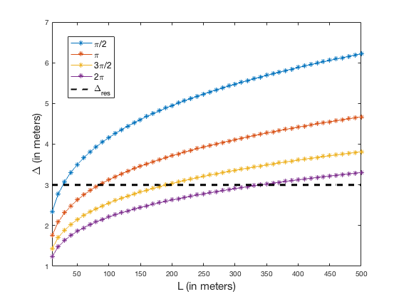
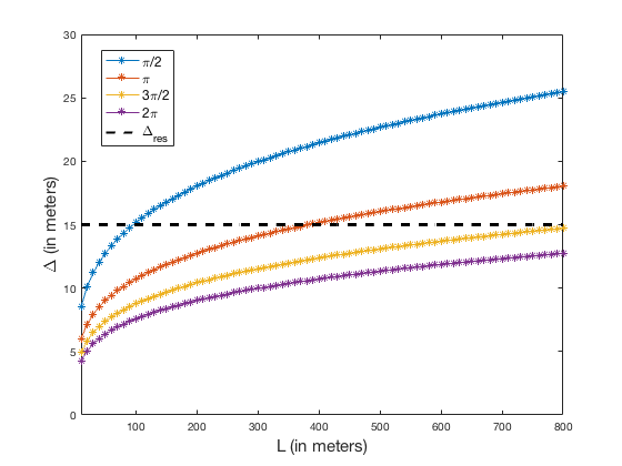
The resolution bound of Corollary 1 corresponds to the super-resolution regime when reconstructing small scenes in both active, and passive scenarios, as depicted in Figure 1(a) and Figure 1(b), respectively. Note that as gets large, the lower bound eventually becomes greater than the range resolution limit of the Fourier-based methods. This is in agreement with our theoretical arguments, which are established under a small scene approximation. It should also be stressed that our lower bound abides by the sufficient condition for exact recovery, but it is not a necessary one. Therefore, while recovery of scenes at a higher resolution than may still be possible via GWF, it is not covered by the theory in [1].
Additionally, the sufficient number of receivers for (29) to hold is . Since by (25), this implies that super-resolution imaging via GWF requires a sample complexity of at least . We reduce this complexity result by the following corollary, which quantifies the minimal sample requirement for exact multi-static imaging via GWF at a fixed pixel spacing that abides the lower bound of Corollary 1 .
Corollary 2 (Sample Complexity).
Given the final result of Theorem 1, exact multistatic imaging condition for GWF is satisfied at the following sample complexity:
| (31) |
Proof.
Reorganizing the upper bound on in Theorem 1, we have
| (32) |
where , are as functions of and . Now, for any fixed pixel spacing , we have . Thus,
| (33) |
for some . Observe that factor in the first term of the left-hand side of (33) is non-vanishing and hence at best yields the RIC upper bound of . Now from Assumption 1, we have . Thus, the minimal sample complexity in which the RIC upper bound is in the order of is achieved when . Therefore,
| (34) |
when . ∎
In addition to the minimal sample complexity, Corollary 2 yields a rate at which the algorithm performance deteriorates. Clearly, from (34), our ability to fine sample the scene while attaining the exact recovery guarantees of GWF for multi-static imaging depends on the dimension of the problem, at a rate , or equivalently, . This, again, is consistent with our theoretical arguments as we derive our results through a small scene approximation.
The fact that the upper bound of has a non-vanishing factor reveals an interesting phenomenon that is also observed in the performance of spectral initialization in phase retrieval literature, even when the measurement vectors are random. This degradation with the increasing dimension of the unknown is not captured in the probabilistic analysis with random measurement vectors, yet is indeed a significant issue which forms the basis for sample truncation in computing the initialization and gradient estimates [50].
Specifically for deterministic, wave-based multistatic imaging problems, Corollary 2 necessitates a system design such that the controllable constants in (34) sufficiently suppress the factor. This promotes GWF as a highly applicable method in passive imaging scenarios where the range resolution is limited, or in active imaging scenarios where small, isolated extended targets are being imaged, with possible extensions and applications in spot-light mode synthetic aperture radar [51].
IV Numerical Simulations
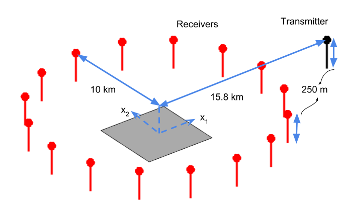
In this section, we provide several numerical simulations demonstrating veracity of the theory presented in Section III. The following multistatic set-up is common to all simulations presented in this section, and conforms to the assumptions laid out in Section III.
-
1.
There is a single transmitter located at km.
-
2.
The transmitted waveform has unit amplitude frequency spectrum.
-
3.
Varying number of receivers are distributed equidistant on an arc of a circle of radius km from the scene center at a height of km.
-
4.
The scene of interest is square with flat topography.
Figure 2 illustrates the multistatic set-up used in this section. Note that the illustration is not to scale.
The figure-of-merit we use throughout is the mean square error (MSE) of the reconstructed scene. This is computed by taking the per pixel difference between the true scene and the reconstructed scene and averaging the squares of the differences.
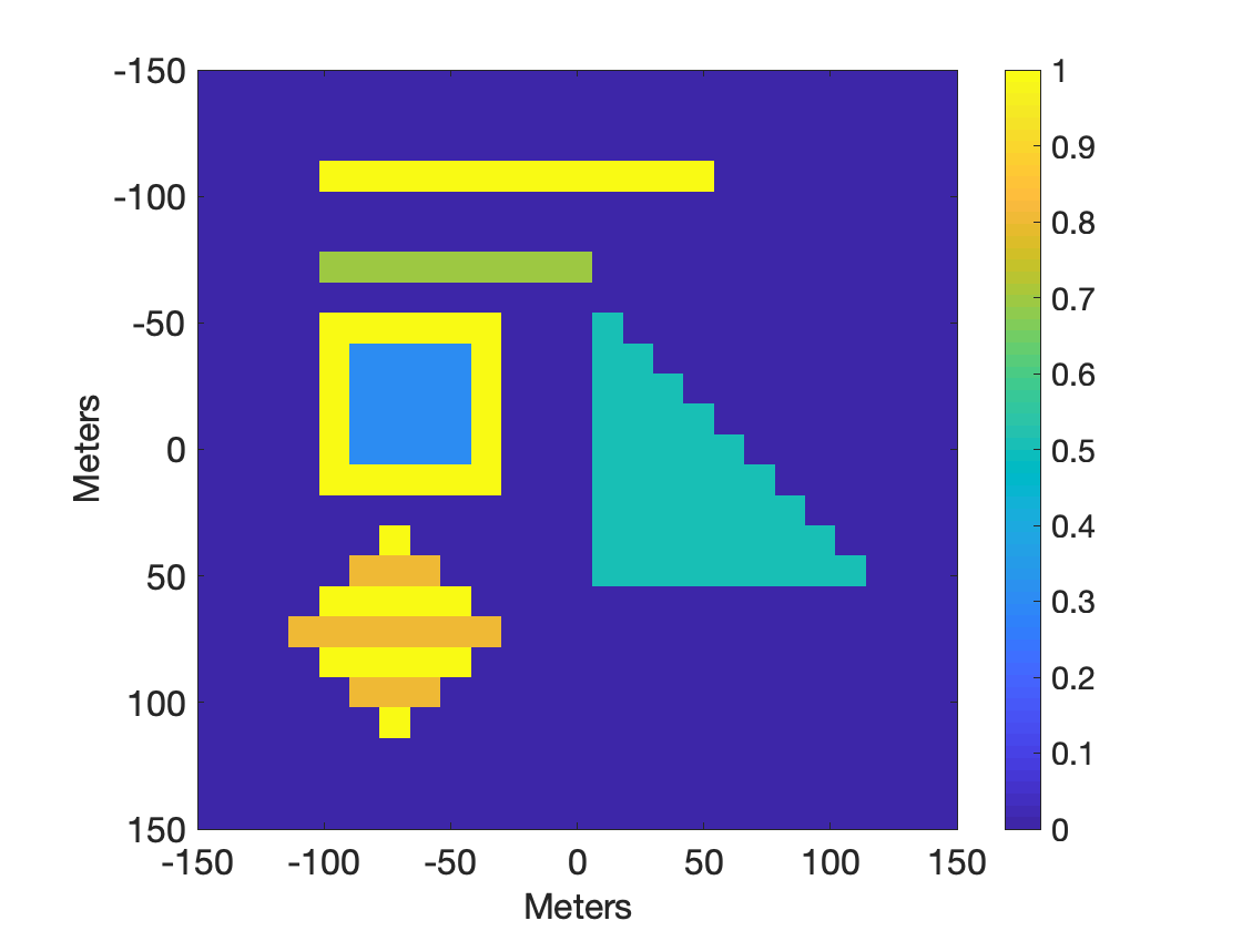
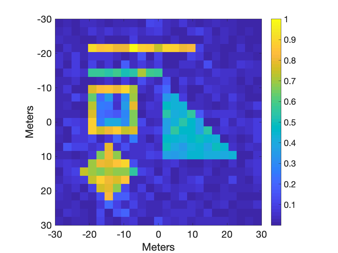
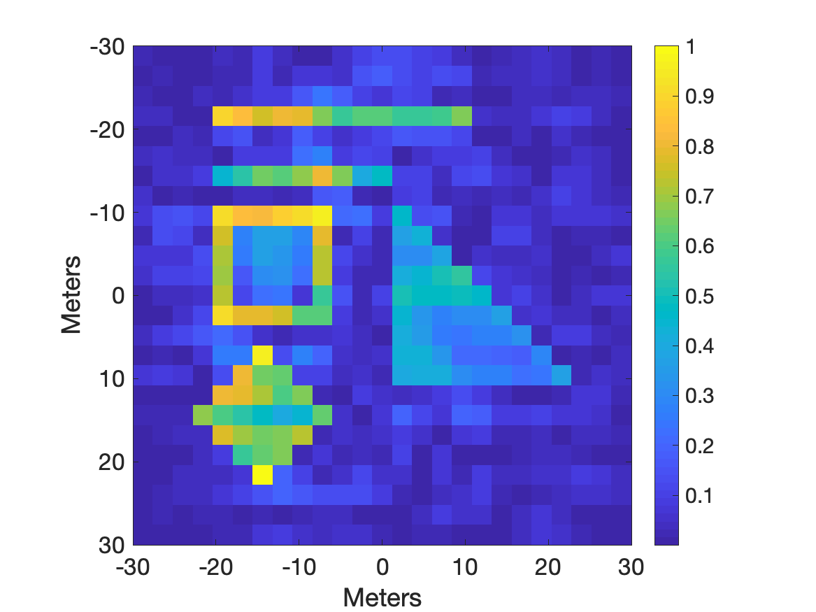
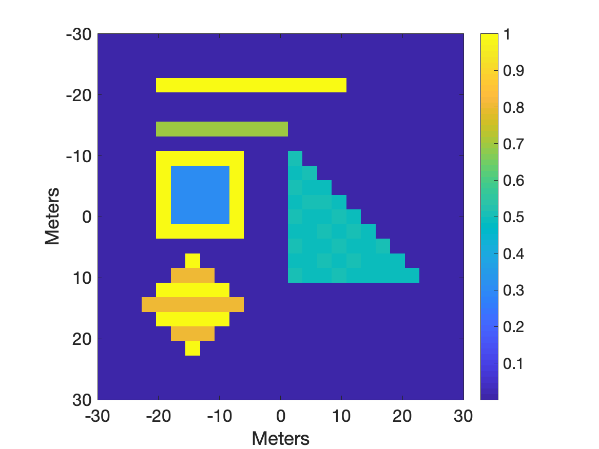
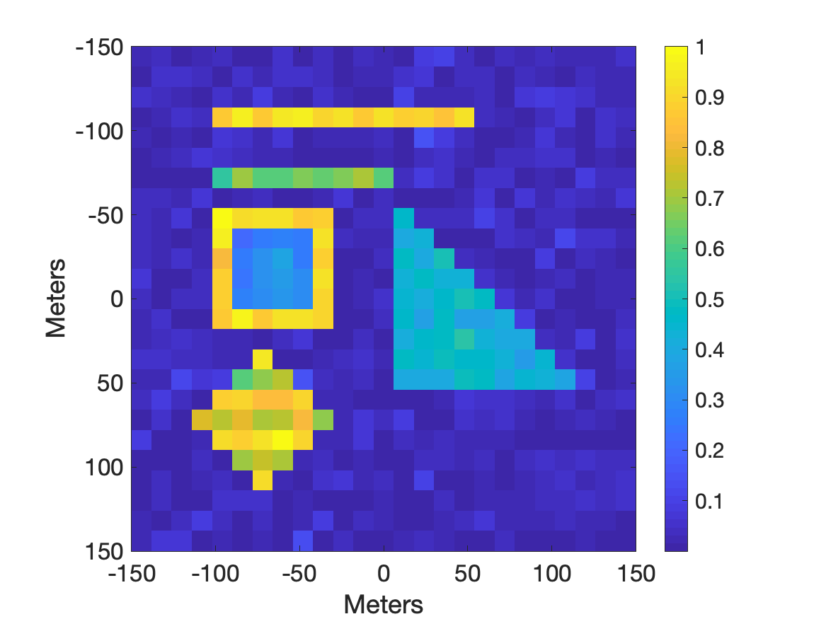
In all experiments presented, our data is synthetically generated using our received signal model in (1) under the single-scattering assumption. In Sections IV-A, IV-B, and IV-C, a single parameter is varied in each set of experiment while all other relevant parameters are fixed. The parameters are chosen in the active and passive imaging ranges. Figure 3 shows the scene used for all experiments in the subsequent sections. Finally, in Section IV-D, we provide simulations that depict the performance of GWF in non-ideal conditions, namely under additive noise at low signal-to-noise ratios (SNR), and discretization mismatch between the ground truth, and the reconstructed image.

IV-A Effect of Number of Receivers
The first series of numerical experiments are designed to verify the effect of the number of receivers on the performance of GWF reconstruction. In (27), the second term involves the square of the number of receivers, , in the denominator. Thus, we expect the number of receivers to have significant effect on the quality of the reconstruction. To verify the effect of the number of receivers on the reconstruction, we ran a series of simulations with varying number of receivers while fixing all other relevant parameters in active or passive radar regimes.
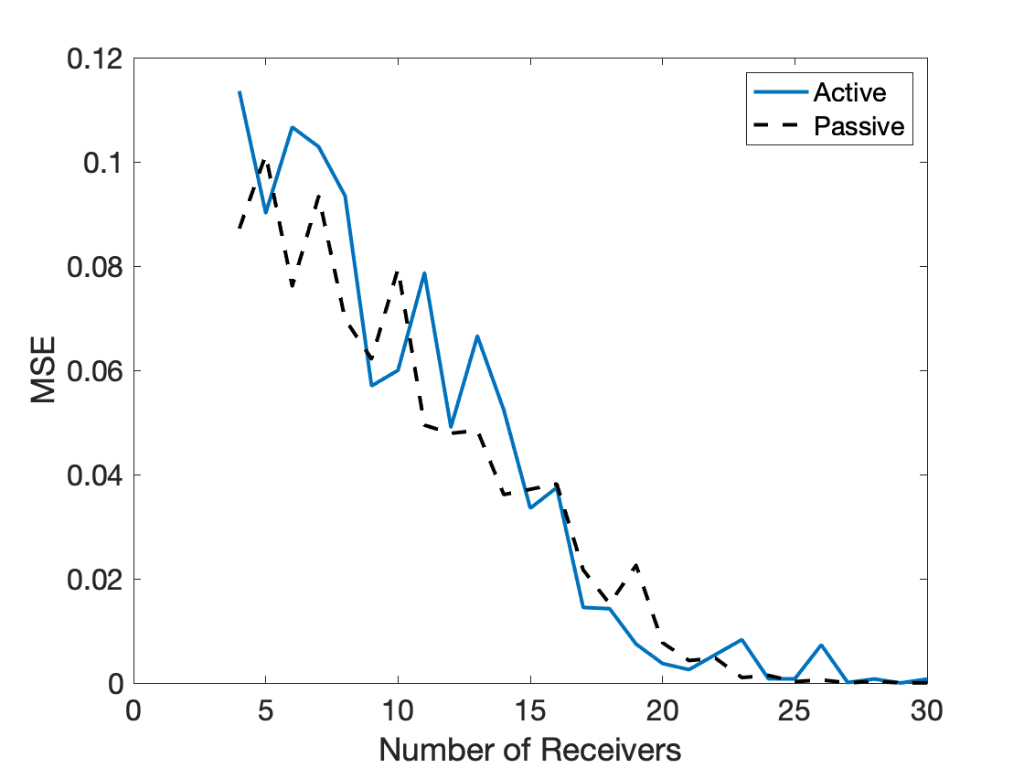
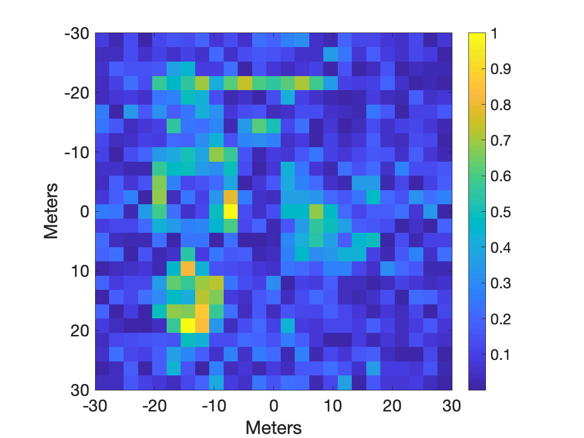
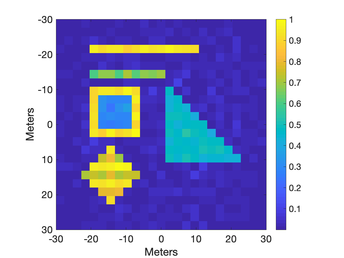
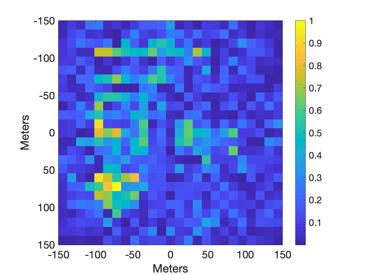

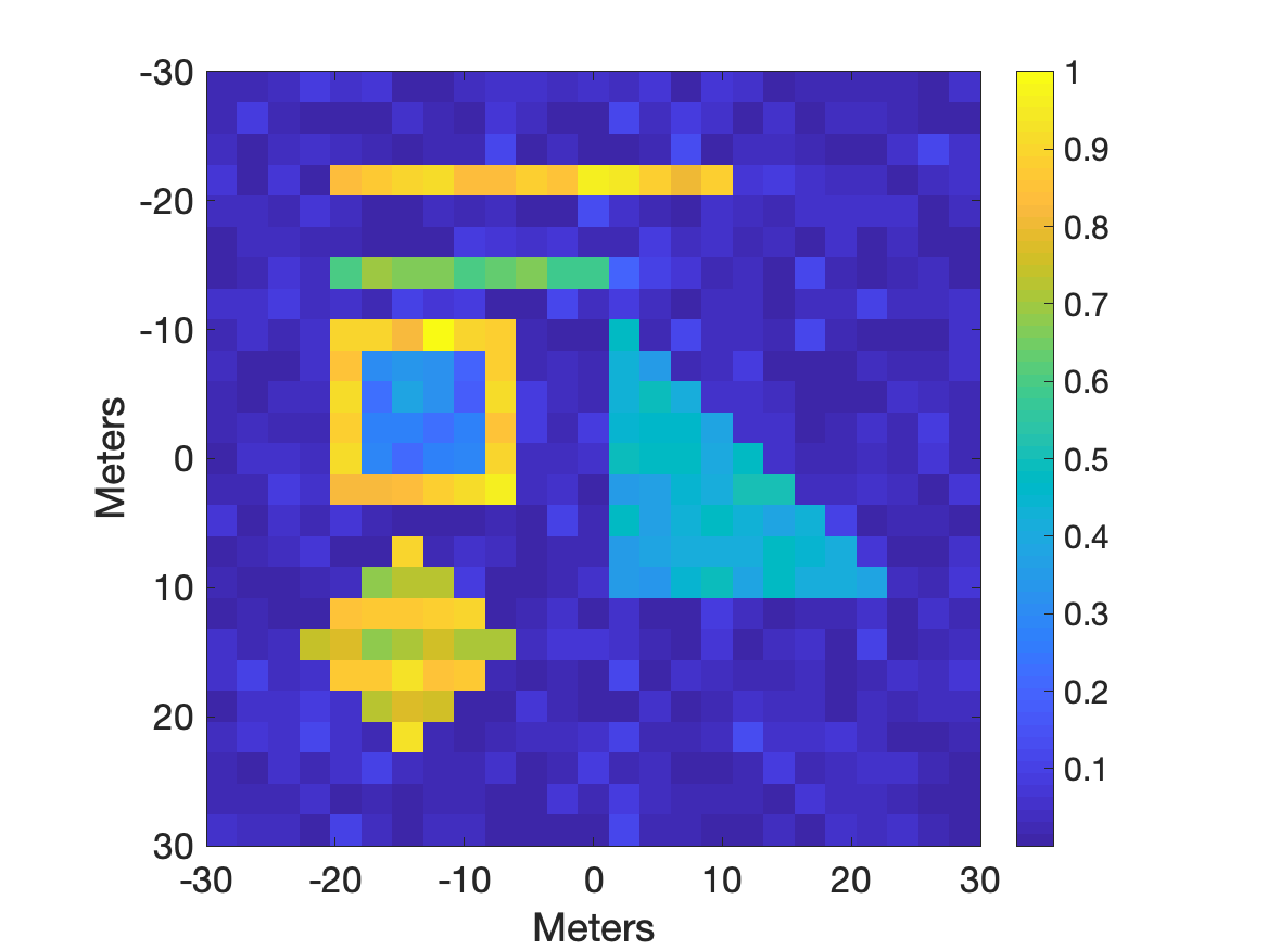
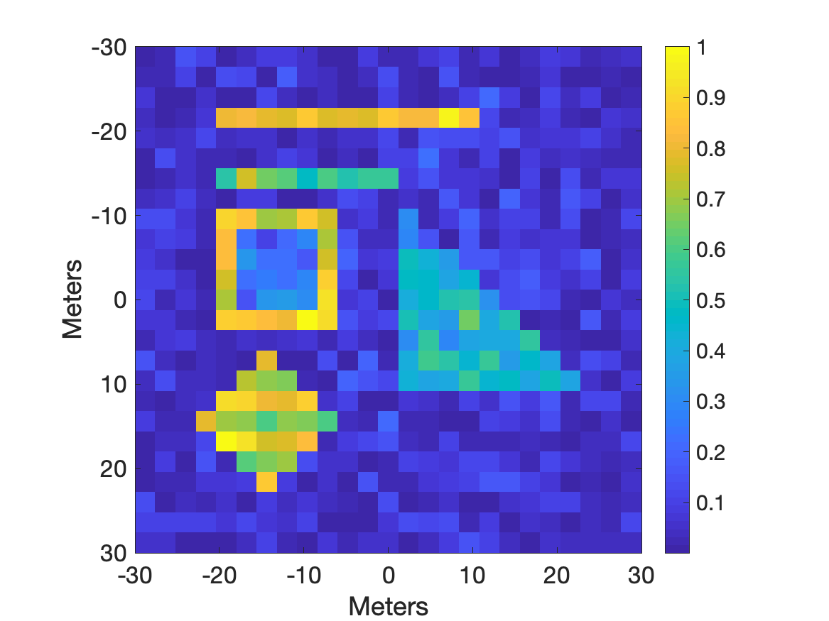
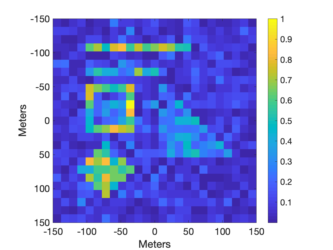
Figure 4 shows the MSE of the resulting reconstruction versus the number of receivers for active and passive imaging. Blue solid line is the result for the active case while black dashed line is for the passive case. For the active case, the bandwidth was held at MHz with the center frequency at GHz for Fourier-based range resolution of m. For the passive case, MHz and GHz for m. The pixel spacing was chosen such that it was smaller than the Fourier-based range resolution for each case. Namely, m and m for the active and passive cases, respectively. The number of unknowns was held constant at for both cases. The GWF algorithm was performed for iterations for comparison purposes. Since the RIC directly affects the rate of convergence of GWF, we expect to see smaller MSE as the number of receivers grows. This behavior is clearly present in both the active and passive cases as can be readily observed in Figure 4. In both cases, we observed exact convergence behavior from receivers onward. However, as expected, the convergence rate is slower with smaller number of receivers.
IV-B Effect of Bandwidth/Range Resolution
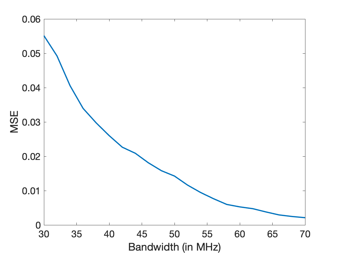


Next we examine the effect of the bandwidth on the convergence behavior. Both terms in (27) includes square root of , the range resolution, in the numerator. This suggests that there is an inverse relationship between the bandwidth and RIC. Similar to above, we test the effect of bandwidth on the convergence behavior of GWF algorithm, and we ran a series of GWF reconstruction on the same scene while varying the bandwidth and holding other relevant parameters fixed. The number of receivers used for the experiments was fixed at . All other parameters were held to the same values as in the previous subsection.
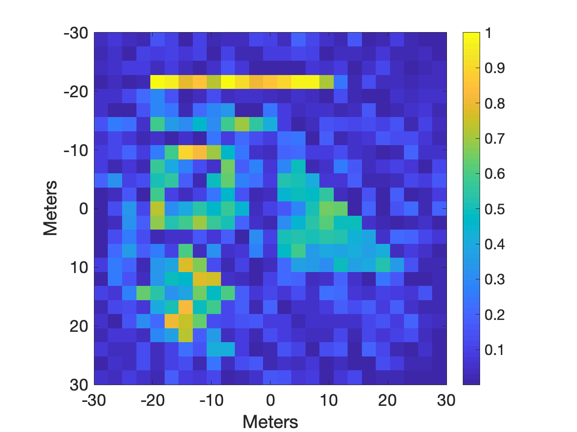
Figure 7 summarizes the result of these experiments. Figure 7(a) shows the bandwidth vs. MSE curve for active case. We varied the bandwidth in the range of MHz to MHz. Figure 7(b) shows the same curve for the passive case where the bandwidth was varied between MHz and MHz. Examining the two figures, we clearly see that higher bandwidth results in smaller MSE, and hence faster convergence to exact solution. This agrees with the theoretical bound in (27). As before, we provide visual confirmation in form of sample reconstructions in Figures 8 and 9 for active and passive regimes, respectively.
IV-C Effect of Center Frequency
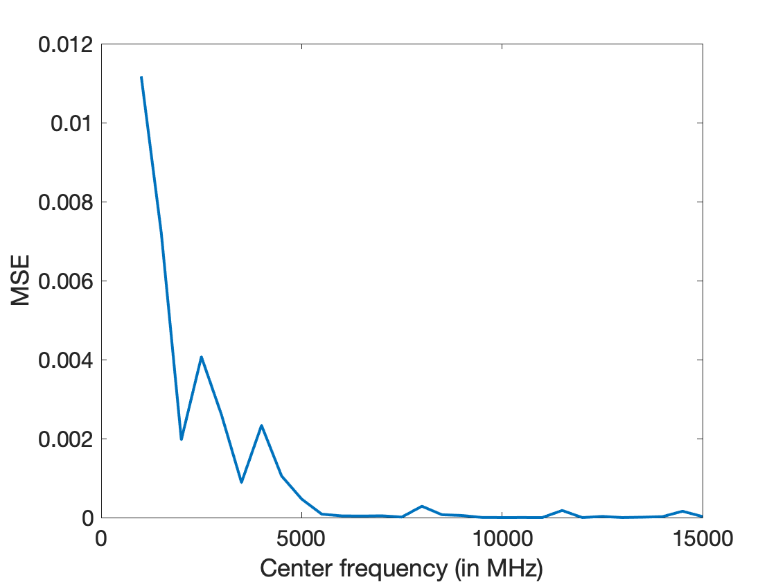
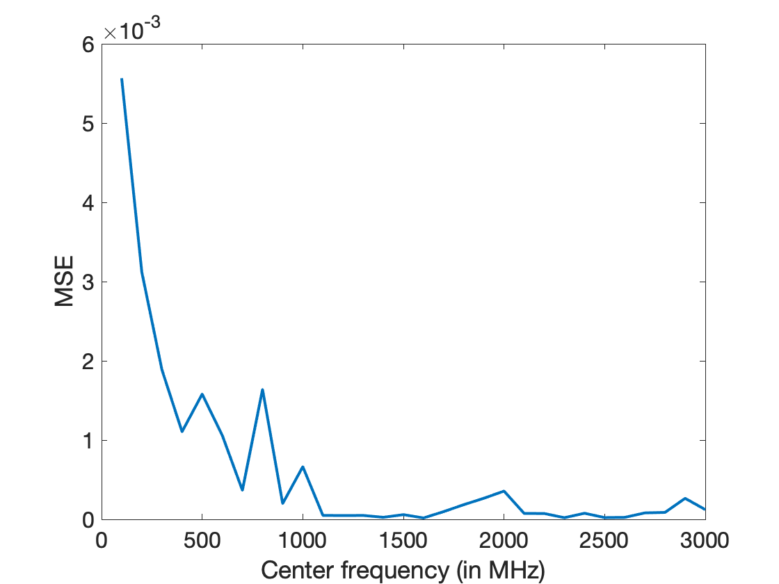


The first term of (27) is inversely proportional to the center frequency of the transmitted waveform and as such we expect the center frequency to improve the convergence behavior of GWF as the center frequency gets larger. We examined numerically, the effect of center frequency on the exact reconstruction and the convergence rate by, again, running a series of numerical simulations where we varied the center frequency while keeping other relevant variables constant. To minimize the effect of the second term on the RIC and better evaluate the impact of central frequency in the super-resolution regime, we increased the number of receivers used in these experiments to for both cases.
Figures 10(a) and 10(b) show the results of simulated experiments for active and passive scenarios, respectively. For active case, we varied the center frequency in the range between GHz and GHz. For the passive case, the range was restricted to GHz to GHz to reflect realistic values for sources of opportunity. In both cases, we observe a behavior of downward trend in MSE as the center frequency increases, albeit, not as drastic as in other parameters. This is due to the fact that the central frequency appears inverted in the two terms of the RIC upper bound. The decaying trend of our experiments agrees with the notion that the order constant of the second term in the RIC upper bound adequately suppresses , as proves to be sufficient for super-resolution.
Notice, however, that in the active case, larger center frequency value is needed to achieve similar performance as in the passive case. This is attributable to the fact that the first term is proportional to . With the active parameters, this term is approximately times that of the passive case. Thus, the center frequency needs to be higher to compensate for the difference. Figures 11 and 12 show sample reconstructions at two different center frequencies for active and passive regimes, respectively.
IV-D Effect of Additive Noise
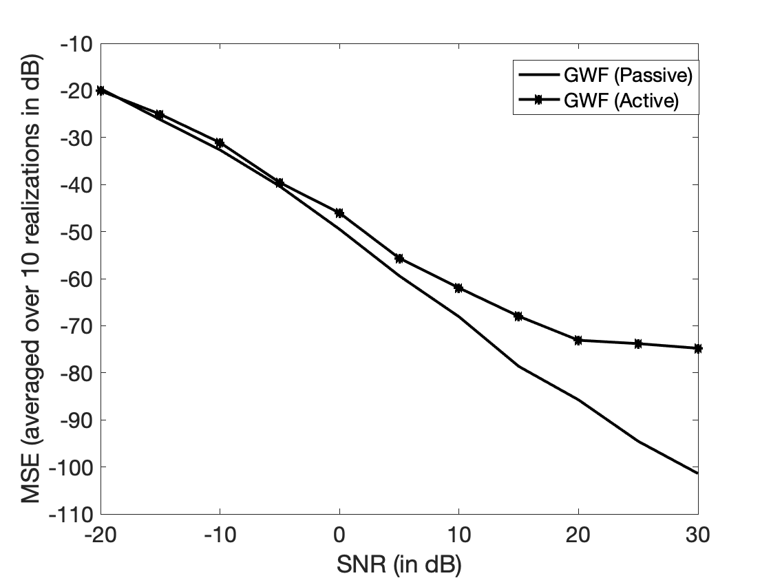


Next, we evaluate the robustness of the proposed method for interferometric multi-static radar imaging, in passive, and active cases. As before, we use a flat spectrum signal with MHz bandwidth centered around GHz frequency in the passive, and a MHz bandwidth centered around GHz frequency in the active experiments. We incorporate additive, zero-mean white Gaussian noise on the linear signal model at the receivers, and consider SNR levels varying from to dB. Figure 13 demonstrates the reconstruction MSE with respect to the received signal SNR with dB increments, with errors averaged over realizations. The MSE curves indicate that GWF is robust to additive noise at the receivers in both active and passive cases, and the performance of the algorithm degrades predictably with decreasing SNRs, with steady decay in MSE as the SNR at the receivers improve.
It should be noted that the correlation operation amplifies the noise variance, hence the interferometric measurements processed in the experiments have lower SNR than the specified levels at the receivers. Nonetheless, we observe that the reconstruction performance of GWF degrades gracefully as SNR decrases, as Figure 14, Figure 15 and Figure 16 demonstrate that GWF is capable of producing highly accurate imagery with dB in the received signals at the antennas. However with SNRs below dB the algorithm performance degrades noticeably, which motivates filtering or sample truncation at the implementation of GWF in low SNR scenarios.
V Conclusion
In this paper, we utilize GWF theory developed in [1] for exact multistatic imaging of extended targets by designing the underlying imaging parameters such that the sufficient condition for exact recovery is satisfied. Our work has two significant contributions. 1) Unlike the state-of-the-art interferometric inversion methods based on LRMR, GWF avoids lifting the problem. As a result, it is computationally efficient and does not require large memory allocations, making it suitable for practical applications. 2) We demonstrate that the underlying imaging parameters can be designed so that the RIP over rank-1, PSD matrices is satisfied by a deterministic lifted forward model.
We first show the asymptotic isometry of the lifted forward model, , of interferometric multistatic radar, as the center frequency and the number of receivers go to infinity. We then proceed with estimating the deviation from the asymptotic behavior when imaging parameters are finite, and derive an upper bound for the RIC of over the set of rank-1, PSD matrices. Hence, we identify the relation of imaging parameters to the sufficient condition of exact recovery. Using the RIC upper bound, we determine a lower limit for pixel spacing to achieve exact recovery. This limit is superior to the Fourier-based range resolution for sufficiently small scenes. Furthermore, we determine the minimal sample complexity needed for RIC upper bound to be sufficiently small, hence identify the practical requirements for reconstruction when designing a multistatic imaging system. In our numerical simulations, we evaluate the impact of the imaging parameters in our upper bound estimate of RIC in reconstruction performance, verify our theoretical results, and finally assess the performance of GWF to additive noise at low SNRs.
For future work, we will study the robustness of our method with respect to deviations from our imaging setup, such as non-equi-distant locations, or non-circular configurations of receivers. In addition, we will investigate extensions of our theory to the case involving additive noise and outliers, moving target imaging, as well as implementation of our method using real scattering data.
References
- [1] B. Yonel and B. Yazici, “A generalization of wirtinger flow for exact interferometric inversion,” arXiv preprint arXiv:1901.03940, 2019, submitted to SIAM Journal on Imaging Sciences.
- [2] E. J. Candes, X. Li, and M. Soltanolkotabi, “Phase retrieval via Wirtinger flow: Theory and algorithms,” IEEE Trans. Inf. Theory, vol. 61, no. 4, pp. 1985–2007, Apr. 2015.
- [3] E. J. Candes, Y. Eldar, T. Strohmer, and V. Voroninski, “Phase retrieval via matrix completion,” SIAM J. Imag. Sci., vol. 6, no. 1, pp. 199–225, 2013.
- [4] E. J. Candes and T. Strohmer, “Phaselift: Exact and stable recovery from magnitude measurements via convex programming,” Commun. Pure and Appl. Math., vol. 66, no. 8, pp. 1241–1274, Aug. 2013.
- [5] O. M. Bucci and G. Franceschetti, “On the spatial bandwidth of scattered fields,” IEEE transactions on antennas and propagation, vol. 35, no. 12, pp. 1445–1455, 1987.
- [6] ——, “On the degrees of freedom of scattered fields,” IEEE transactions on Antennas and Propagation, vol. 37, no. 7, pp. 918–926, 1989.
- [7] C. E. Yarman and B. Yazici, “Synthetic aperture hitchhiker imaging,” IEEE Trans. Image Process., vol. 17, no. 11, pp. 2156–2173, Nov. 2008.
- [8] J. Garnier and G. Papanicolaou, “Passive sensor imaging using cross correlations of noisy signals in a scattering medium,” SIAM Journal on Imaging Sciences, vol. 2, no. 2, pp. 396–437, 2009.
- [9] L. Wang, I.-Y. Son, and B. Yazici, “Passive imaging using distributed apertures in multiple-scattering environments,” IOP Inverse Problems J., vol. 26, no. 6, pp. 1–37, June 2010.
- [10] H. Ammari, J. Garnier, and W. Jing, “Passive array correlation-based imaging in a random waveguide,” Multiscale Modeling & Simulation, vol. 11, no. 2, pp. 656–681, 2013.
- [11] E. Mason, I.-Y. Son, and B. Yazıcı, “Passive synthetic aperture radar imaging using low-rank matrix recovery methods,” IEEE J. Sel. Topics Signal Process., vol. 9, no. 8, pp. 1570–1582, Dec. 2015.
- [12] J. Garnier, “Imaging in randomly layered media by cross-correlating noisy signals,” Multiscale Modeling & Simulation, vol. 4, no. 2, pp. 610–640, 2005.
- [13] O. I. Lobkis and R. L. Weaver, “On the emergence of the green’s function in the correlations of a diffuse field,” The Journal of the Acoustical Society of America, vol. 110, no. 6, pp. 3011–3017, 2001.
- [14] L. Borcea, G. Papanicolaou, and C. Tsogka, “Theory and applications of time reversal and interferometric imaging,” Inverse Problems, vol. 19, no. 6, p. S139, 2003.
- [15] ——, “Interferometric array imaging in clutter,” Inverse Problems, vol. 21, no. 4, p. 1419, 2005.
- [16] ——, “Coherent interferometric imaging in clutter,” Geophysics, vol. 71, no. 4, pp. SI165–SI175, 2006.
- [17] P. Blomgren, G. Papanicolaou, and H. Zhao, “Super-resolution in time-reversal acoustics,” The Journal of the Acoustical Society of America, vol. 111, no. 1, pp. 230–248, 2002.
- [18] P. Gough and M. Miller, “Displaced ping imaging autofocus for a multi-hydrophone sas,” IEE Proceedings-Radar, Sonar and Navigation, vol. 151, no. 3, pp. 163–170, 2004.
- [19] S. Flax and M. O’Donnell, “Phase-aberration correction using signals from point reflectors and diffuse scatterers: Basic principles,” IEEE transactions on ultrasonics, ferroelectrics, and frequency control, vol. 35, no. 6, pp. 758–767, 1988.
- [20] E. Mason and B. Yazici, “Robustness of lrmr based passive radar imaging to phase errors,” in EUSAR 2016: 11th European Conference on Synthetic Aperture Radar, Proceedings of, 2016, pp. 1–4.
- [21] R. Novikov, “Formulas for phase recovering from phaseless scattering data at fixed frequency,” Bulletin des Sciences Mathématiques, vol. 139, no. 8, pp. 923–936, 2015.
- [22] P. Bardsley and F. G. Vasquez, “Kirchhoff migration without phases,” Inverse Problems, vol. 32, no. 10, p. 105006, 2016.
- [23] Z. Chen and G. Huang, “Phaseless imaging by reverse time migration: acoustic waves,” Numerical Mathematics: Theory, Methods and Applications, vol. 10, no. 1, pp. 1–21, 2017.
- [24] A. Novikov, M. Moscoso, and G. Papanicolaou, “Illumination strategies for intensity-only imaging,” SIAM Journal on Imaging Sciences, vol. 8, no. 3, pp. 1547–1573, 2015.
- [25] J. Laviada, A. Arboleya-Arboleya, Y. Alvarez-Lopez, C. Garcia-Gonzalez, and F. Las-Heras, “Phaseless synthetic aperture radar with efficient sampling for broadband near-field imaging: Theory and validation,” IEEE Transactions on Antennas and Propagation, vol. 63, no. 2, pp. 573–584, 2014.
- [26] L. Wang, C. E. Yarman, and B. Yazici, “Doppler-Hitchhiker: A novel passive synthetic aperture radar using ultranarrowband sources of opportunity,” IEEE Trans. Geosci. Remote Sens., vol. 49, no. 10, pp. 3521–3537, Oct. 2011.
- [27] L. Wang and B. Yazici, “Passive imaging of moving targets exploiting multiple scattering using sparse distributed apertures,” IOP Inverse Problems J., vol. 28, no. 12, pp. 1–36, Dec. 2012.
- [28] ——, “Passive imaging of moving targets using sparse distributed apertures,” SIAM J. Imag. Sci., vol. 5, no. 3, pp. 769–808, 2012.
- [29] S. Wacks and B. Yazici, “Passive synthetic aperture hitchhiker imaging of ground moving targets - Part 1: Image formation and velocity estimation,” IEEE Trans. Image Process., vol. 23, no. 6, pp. 2487–2500, June 2014.
- [30] D. Kissinger, “Radar fundamentals,” in Millimeter-Wave Receiver Concepts for 77 GHz Automotive Radar in Silicon-Germanium Technology. Boston, MA. USA: Springer US, 2012, pp. 9–19.
- [31] L. Demanet and V. Jugnon, “Convex recovery from interferometric measurements,” IEEE Trans. Comput. Imag., vol. 3, no. 2, June 2017.
- [32] I. Waldspurger, A. d’Aspremont, and S. Mallat, “Phase recovery, maxcut and complex semidefinite programming,” Math. Program., vol. 149, no. 1-2, pp. 47–81, Feb. 2015.
- [33] A. Chai, M. Moscoso, and G. Papanicolaou, “Array imaging using intensity-only measurements,” IOP Inverse Problems J., vol. 27, no. 1, pp. 1–16, Jan. 2011.
- [34] B. Recht, M. Fazel, and P. Parrilo, “Guaranteed minimum-rank solutions of linear matrix equations via nuclear norm minimization,” SIAM Rev., vol. 52, no. 3, pp. 471–501, 2010.
- [35] A. M. Haimovich, R. S. Blum, and L. J. Cimini, “Mimo radar with widely separated antennas,” IEEE Signal Processing Magazine, vol. 25, no. 1, pp. 116–129, 2008.
- [36] V. S. Chernyak, Fundamentals of multisite radar systems: multistatic radars and multistatic radar systems. New York, NY: Gordon and Breach, 1998.
- [37] H. Lev-Ari and A. J. Devancy, “The time-reversal technique re-interpreted: subspace-based signal processing for multi-static target location,” in Proceedings of the 2000 IEEE Sensor Array and Multichannel Signal Processing Workshop. SAM 2000 (Cat. No.00EX410), March 2000, pp. 509–513.
- [38] L. Griffiths and C. Jim, “An alternative approach to linearly constrained adaptive beamforming,” IEEE Transactions on Antennas and Propagation, vol. 30, no. 1, pp. 27–34, January 1982.
- [39] C. Prada and M. Fink, “Eigenmodes of the time reversal operator: A solution to selective focusing in multiple-target media,” Wave Motion, vol. 20, no. 2, pp. 151 – 163, 1994. [Online]. Available: http://www.sciencedirect.com/science/article/pii/0165212594900396
- [40] A. Paulraj, B. Ottersten, R. Roy, A. Swindlehurst, G. Xu, and T. Kailath, “Subspace methods for directions-of-arrival estimation,” in Handbook of Statistics. Elsevier, 1993, vol. 10, pp. 693–739.
- [41] A. Kirsch, “Characterization of the shape of a scattering obstacle using the spectral data of the far field operator,” Inverse Problems, vol. 14, no. 6, pp. 1489–1512, dec 1998.
- [42] A. Kirsch and S. Ritter, “A linear sampling method for inverse scattering from an open arc,” Inverse Problems, vol. 16, no. 1, pp. 89–105, jan 2000.
- [43] T. Arens and A. Lechleiter, “The linear sampling method revisited,” The Journal of Integral Equations and Applications, pp. 179–202, 2009.
- [44] D. Strong and T. Chan, “Edge-preserving and scale-dependent properties of total variation regularization,” Inverse problems, vol. 19, no. 6, p. S165, 2003.
- [45] Y. Yu, A. P. Petropulu, and H. V. Poor, “Mimo radar using compressive sampling,” IEEE Journal of Selected Topics in Signal Processing, vol. 4, no. 1, pp. 146–163, Feb 2010.
- [46] M. A. Herman and T. Strohmer, “High-resolution radar via compressed sensing,” IEEE Transactions on Signal Processing, vol. 57, no. 6, pp. 2275–2284, June 2009.
- [47] K.-T. Kim, D.-K. Seo, and H.-T. Kim, “Efficient radar target recognition using the music algorithm and invariant features,” IEEE Transactions on Antennas and Propagation, vol. 50, no. 3, pp. 325–337, March 2002.
- [48] L. Audibert and H. Haddar, “The generalized linear sampling method for limited aperture measurements,” SIAM Journal on Imaging Sciences, vol. 10, no. 2, pp. 845–870, 2017.
- [49] M. Cheney and B. Borden, Fundamentals of radar imaging. Siam, 2009, vol. 79.
- [50] Y. Chen and E. J. Candes, “Solving random quadratic systems of equations is nearly as easy as solving linear systems,” Communications on Pure and Applied Mathematics, vol. 70, pp. 0822–0883, 2017.
- [51] B. Yonel, E. Mason, and B. Yazici, “Phaseless passive synthetic aperture radar imaging via wirtinger flow,” in 2018 52nd Asilomar Conference on Signals, Systems, and Computers. IEEE, 2018, pp. 1623–1627.
- [52] W. Rudin, Real and Complex Analysis, 3rd Ed. New York, NY, USA: McGraw-Hill, Inc., 1987.
Appendix A Proofs
A-A Proof of Lemma 1
We first examine the -norm of the data. For a rank- , we have that . We can also rewrite
| (35) |
Thus, from (11), (8), and (9) we have
| (36) | ||||
Similarly, we have that
| (37) | ||||
where is as in (15).
Then, under Assumption 1, we have that
| (38) | ||||
where . The second line is from geometric sum and the last line is from small angle approximation.
A-B Proof of Proposition 1
First we express as
| (43) | ||||
where
| (44) | ||||
Given (43), it suffices to prove that
| (45) | ||||
| (46) |
This can be proved using similar machinery to proving the delta function limit for sequence of scaled sinc functions. We prove the first equation (45). The second equation follows similarly.
Let be a smooth test function, where is the Schwartz space. Then we need to prove that
| (47) |
where
| (48) |
Let and break-up the integral into two parts.
| (49) | ||||
The first part of the integral is
| (50) | ||||
We compute the first part of (50). Integrating by parts,
| (51) | ||||
Since , taking the limit as , (51) goes to . Similarly, we can see that the second integral in (50) also goes to zero. Thus,
| (52) |
Now, the second integral in (49) can be rewritten as
| (53) |
The first integral can be rewritten as
| (54) |
Since , we can use Riemann-Lebesgue lemma to conclude that (54) goes to zero as [52].
For second integral, we have
| (55) |
After change of variables , we have
| (56) |
as . We can use similar argument for where
| (57) |
A-C Proof of Proposition 2
Without loss of generality, let the receivers and transmitters have common elevation angle such that
| (58) | ||||
| (59) |
where is the azimuth angle of the -th receivers look-direction, is the azimuth angle of the transmitter look-direction and is the elevation angle. Furthermore, we have that for any and
| (60) |
where is the angle of the vector . Then we have that
| (61) | ||||
Thus, for the non-diagonal terms where , we have that if
| (62) | ||||
For fixed and , there are at most values of ’s for which (62) is satisfied. Furthermore, we know that ’s must be bounded. Thus, by Proposition 1, for each fixed where and we have that
| (63) |
Now taking the limit as , we have the desired result.
A-D Proof of Theorem 1
We want to upper bound the following
| (64) | ||||
where, by Assumption 3. Without loss of generality we set . We begin by noting that
| (65) |
where
| (66) |
Thus, fixing , , and , we have convolution between and . Let
| (67) |
We take the Fourier Transform of and to represent the convolution. Denoting, as the Fourier Transform of , we have
| (68) | ||||
To compute , we first rewrite as
| (69) | ||||
Let , and be the azimuth angle of the -th receiver’s look-direction. Then, given (69), the Fourier Transform of and using the assumption that ,
| (70) |
where
| (71) |
| (72) | ||||
and
| (73) |
Noting that is only non-zero where , and , we approximate (71) as
| (74) |
Next, we note that
| (75) |
Thus, interchanging the sum and the integral in (68), and plugging in (70) we have
| (76) | ||||
| (77) |
where
| (78) | ||||
| (79) |
Now, by employing Cauchy-Schwartz, we have
| (80) | ||||
where
| (81) |
By Jensen’s inequality, (80) becomes
| (82) | |||
| (83) |
Noting that for any fixed ,
| (84) |
we have
| (85) | ||||
We use Jensen’s inequality once more to get
| (86) | ||||
Next, approximating the sum over as an integral, we have
| (87) | ||||
where denotes the Riemann sum error, is the aperture of look directions in the imaging setup.
We first consider the inner integration over , where . Using Cauchy-Schwartz and Jensen’s inequalities,
| (88) |
Computing the first integral in (88), we get
| (89) |
Consider the second integral in (88). Since the integrand is strictly positive, from the integration we have
| (90) |
We now make the following change of variables
| (91) |
Computing the Jacobian, we get
| (92) |
Thus, setting , the upper bound in (90) becomes
| (93) |
where the last identity follows from Parseval’s theorem. Hence, we obtain the upper bound on our integral approximation, i.e., the first term in (87) as
| (94) |
We next evaluate the error term of the integral approximation in (93). Namely, the midpoint Riemann-sum approximation error is upper bounded as
| (95) |
where is defined as
| (96) |
using the definition of .
Since the integrand is the squared absolute value of the Fourier transform of the reflectivity function evaluated at frequencies , (96) can equivalently be written as
| (97) |
which is the form of a Frobenius inner product, where
| (98) |
Observe that has an upper bound that only depends on the norm of the underlying scene as
| (99) |
and that has only dependence on the imaging system, hence yields a universal upper bound for any scene reflectivity function in the specific imaging geometry. Evaluating the integral in (98) and having , can be approximated under the narrow-band assumption as
| (100) |
Denoting , the second order derivative of each component in with respect to is obtained as
| (101) |
where
| (102) |
By definition, the amplitude of sinc-function derivatives in (101) have a decay rate of , whereas and its derivatives in (101) grow with an order of the scene dimension , as . Hence, evaluating the squared integral for the Frobenius norm, the growth is at a maximal order of . We thereby obtain a final approximate upper bound on the universal constant as
| (103) |
Putting the terms derived in (103) and (94) into (86) and (77), we have
| (104) |
for the definition of in Definition 1, using the fact that for the rank-1, PSD element .