A Polynomial-Based Approach for Architectural Design and Learning with Deep Neural Networks

Abstract

In this effort we propose a novel approach for reconstructing multivariate functions from training data, by identifying both a suitable network architecture and an initialization using polynomial-based approximations. Training deep neural networks using gradient descent can be interpreted as moving the set of network parameters along the loss landscape in order to minimize the loss functional. The initialization of parameters is important for iterative training methods based on descent. Our procedure produces a network whose initial state is a polynomial representation of the training data. The major advantage of this technique is from this initialized state the network may be improved using standard training procedures. Since the network already approximates the data, training is more likely to produce a set of parameters associated with a desirable local minimum. We provide the details of the theory necessary for constructing such networks and also consider several numerical examples that reveal our approach ultimately produces networks which can be effectively trained from our initialized state to achieve an improved approximation for a large class of target functions.

1 Introduction

Deep neural networks (DNNs) have emerged as powerful nonlinear approximation tools and have been deployed with great success in many challenging tasks such as image classification [1], playing games, such as Go, at a world-class level [2], and even to produce examples which fool other classifiers [3]. However, DNNs are also known to be difficult to train [4]. Each deep network has its own set of hyper-parameters which must be defined, e.g., the number of layers, the number of nodes per layer, and the connectivity between the nodes on different layers. Ideally, the choice of these parameters is made with respect to the available training data and the task to be solved by the network. In this paper we identify suitable deep network architectures, based on polynomials. Gradient descent-based training procedures are known to be effective for identifying good network parameters [5]. However, such algorithms are sensitive to the initial set of parameters. In addition to identifying suitable network architectures, based on training data, we provide an initialization of parameters so that they perform at least as well as a given polynomial approximation of the training data. This paper establishes an explicit relationship between polynomial approximation and approximation by a neural network and shows that certain network architectures can perform at least as well as any given polynomial-based approach. We also provide numerical examples showing our network not only produces a good approximation but also that our initialization makes training more efficient.

From a high level perspective, every task that a neural network solves can be characterized as a function approximation problem. For example, consider the classification of the ImageNet data set [6], which is composed of many images which fall into one of many possible classes. A typical approach to solve this problem is to choose $k$ classes of images and to train a classifier whose input is an image and whose output is a vector of $k$ probabilities. Each component of the output vector represents the probability that the input belongs to the class corresponding to the component. Therefore, the task is solved by finding a suitable function from a very high dimensional space to a $k$-dimensional space. Classical approximations, that utilize a basis or frame, have a long and very successful history in many diverse areas of science. As such, by constructing networks which achieve comparable performance to polynomial approximations we can explore how neural network approximations relate to other forms of classical, but highly non-linear approximation, such as $n$-term approximations, dictionary approaches, etc.

As Neural networks begin to be integrated into fault intolerant real-world systems, such as self driving cars [7], understanding the error between the network and the desired task/function is vital. Moreover, since it is known that neural networks are universal approximators [8, 9], it is clear that one can build and train an arbitrarily accurate network given enough samples of the target function and given the ability to construct a network as large as desired. There has been extensive research into constructing approximations by classical functions and, in particular, polynomials, see, e.g., [10]. Moreover, these constructive approximations have sharp convergence rates associated with their errors in a variety of norms. Such results may be helpful for creating neural networks which obtain high fidelity approximation of a target function. Therefore, by initializing a network to have the same behavior as a high-fidelity approximating polynomial, we not only have a network whose error is well understood, but also can further train the network to possibly achieve an even more accurate approximation.

In what follows, we propose a network architecture with a sufficient number of nodes and layers so that it can express much more complicated functions than the polynomials used to initialize it. In Section 2 we outline the construction of two networks which approximate polynomials. The first can approximate a given polynomial. Numerical examples which show the performance of this network for approximating a target function are given in Section 3 where we initialize a network to a polynomial approximation of the training set and then train it to achieve better performance. The architecture of the first network constructed in Section 2 is not necessarily the same as those used in practice. It is composed of many simple but separate sub-networks. However, the second network we construct, associated with a specific polynomial, is a deep, feed-forward network with the same number of nodes on each of its hidden layers. Such an architecture is widely used and in Section 3 we show that our polynomial-based initialization allows for easier training and better performance for approximating a given target function.

Related Work

Several other efforts have considered constructing networks which achieve polynomial behavior [11, 12, 13] wherein networks are constructed that approximate polynomials associated with sparse grids, Taylor polynoimals and generalized polynomial chaos approximations. The network presented in this paper is a slightly modified one presented in [12]. Those authors constructed a network which approximates the product of $n$ inputs and used this network to compute multivariate Taylor polynomials. Choosing suitable initialization of network parameters was considered in [14]. A random initialization scheme which avoids common training failures was presented in [15].

2 A Network which Approximates a Polynomial

In this section, we construct a network which approximates a given polynomial arbitrarily well and consider a specific example which is implementable by a deep, feed-forward architecture. Our network will be able to approximate $d$-dimensional polynomials of the form

$$F(\vec{x})=\sum_{\vec{\nu}\in\Lambda}c_{\vec{\nu}}\Psi_{\vec{\nu}}(\vec{x})$$ (1)

where $\vec{x}\in\mathbb{R}^{d}$, $\vec{\nu}\in\mathbb{N}_{0}^{d}$ is a multi-index, $\Lambda$ is a finite set of cardinality $N$, and $c_{\vec{\nu}}$ is the coefficient associated with the polynomial $\Psi_{\vec{\nu}}$, which is a tensor product of one-dimensional polynomials. Each polynomial in the sum in (1) is assumed to be of the form,

$$\Psi_{\vec{\nu}}(\vec{x})=\prod_{i=1}^{d}\psi_{\nu_{i}}(x_{i})$$ (2)

where $\vec{\nu}=(\nu_{1},\dots,\nu_{d})$, and $\psi_{\nu_{i}}$ is a single variable polynomial of degree $\nu_{i}\in\mathbb{N}_{0}$. The polynomial in (2) can be computed by finding the product of $d$ numbers, and, by the fundamental theorem of algebra, $\psi_{\nu_{i}}(x_{i})$ can be computed by a product of $\nu_{i}$ possibly complex numbers. That is,

$$\psi_{\nu_{i}}(x_{i})=a_{i}\prod_{k=1}^{\nu_{i}}\left(x_{i}-r_{k}^{(\nu_{i})}\right)$$ (3)

where the numbers $r_{k}^{(\nu_{i})}\in\mathbb{C}$ are called the roots of the polynomial $\psi_{\nu_{i}}(x_{i})$ and $a_{i}$ is a scaling factor. Hence,

$$\Psi_{\vec{\nu}}(\vec{x})=\prod_{i=1}^{d}a_{i}\prod_{k=1}^{\nu_{i}}\left(x_{i}-r_{k}^{(\nu_{i})}\right).$$ (4)

Without loss of generality, we will focus on the case when the polynomials $\psi_{\nu_{i}}$ have real roots, which is a reasonable restriction since all orthogonal, univariate polynomials have real roots. Moreover, these polynomials can be used to form a basis for polynomials with complex roots in which the polynomial with complex roots can be represented exactly.

Before going into the details we outline the general construction of a network $\tilde{F}$ which approximates $F$. An illustration of its structure is depicted in Figure 2 (b).

1. Choose a family of univariate polynomials $\{\phi_{i}\}_{i=1}^{\infty}$, such as the Legendre polynomials.

2. Find an approximation of the training data $\{(\vec{x}_{j},F(\vec{x}_{j})\}_{j=1}^{M}$ in the tensor product basis generated by $\{\psi_{i}\}$ with $N$-terms associated with a chosen index set $\Lambda$ by identifying the coefficients $c_{\vec{\nu}}$.

3. Find the necessary roots $r_{k}^{(\nu_{i})}$ from (4) and values $a_{i}$.

4. The first layer of the network takes the inputs $\vec{x}$ and sends them to a linear layer with $\sum_{\nu\in\Lambda}\|\vec{\nu}\|_{1}$ nodes each of which computes $x_{i}-r^{(\nu_{i})}$.

5. These values are then used as inputs to sub-networks $\tilde{\Psi}_{\vec{\nu}_{i}}$ which approximate the product polynomial $\Psi$ given by (2).

6. The output weights are set to be the coefficients $c_{\vec{\nu}}$ and the product polynomial is then approximated by the linear combination of the outputs of each of the product blocks $\tilde{\Psi}_{\vec{\nu}_{i}}$.

In light of (4), approximating the polynomial $\Psi_{\vec{\nu}_{j}}(\vec{x})$ can be accomplished by constructing a network that computes the product of $\|\vec{\nu}\|_{1}:=\nu_{1}+\nu_{2}+\cdots+\nu_{d}$ numbers. Such a network can constructed by first constructing a network which computes the product of $2$ numbers. Copies of these sub-networks can be chained together $n-1$ times to produce the product of $n$ numbers. This approach was used in [12] where a series of smaller sub-networks $\tilde{p}(x_{i},x_{j})$ which approximate the product $x_{i}x_{j}$ were arranged into a binary tree in order to compute the product of $n$ numbers. The network $\tilde{p}$ is constructed by noting that

$$x_{i}x_{j}=\frac{1}{2}\left((x_{i}+x_{j})^{2}-x_{i}^{2}-x_{j}^{2}\right)$$

so that the desired product can be approximated by a linear combination of networks which approximate $x\mapsto x^{2}$. A network for such a mapping has been constructed in [16, 13, 12] but only for inputs on the interval $[0,1]$.

These networks are not suitable for computing the product polynomial given by 4. Assume that $\vec{x}\in[a,b]^{d}$. Recall that if the $\phi_{\nu_{i}}$’s are orthonormal, univariate polynomials on $[a,b]$ then their roots are real, in the interval $[a,b]$, and we have that $2a\leq\left|x_{i}-r_{k}^{(\nu_{i})}\right|\leq 2b$. In order to compute a polynomial (4), we need to ensure that the product of numbers in the interval $\left[(2a)^{|\vec{\nu}_{j}|},(2b)^{|\vec{\nu}_{j}|}\right]$ can be computed. However, the same network architecture, as depicted in Figure 1 (a), used in [13, 12] can be used to approximate $x^{2}$ on a general interval $[a,b]$ by changing the network parameters. The following proposition establishes the existence of sucha network and gives explicit parameters so that the network can be constructed.

Proposition 1.

A network $\tilde{f}$ with $L$ hidden layers and $4$ nodes on each layer can approximate the function $f(x)=x^{2}$ on the interval $[a,b]$ with

$$\sup_{x\in[a,b]}|x^{2}-\tilde{f}|\leq\frac{C}{2^{2L}},$$

where $C=(b-a)^{2}/4$.

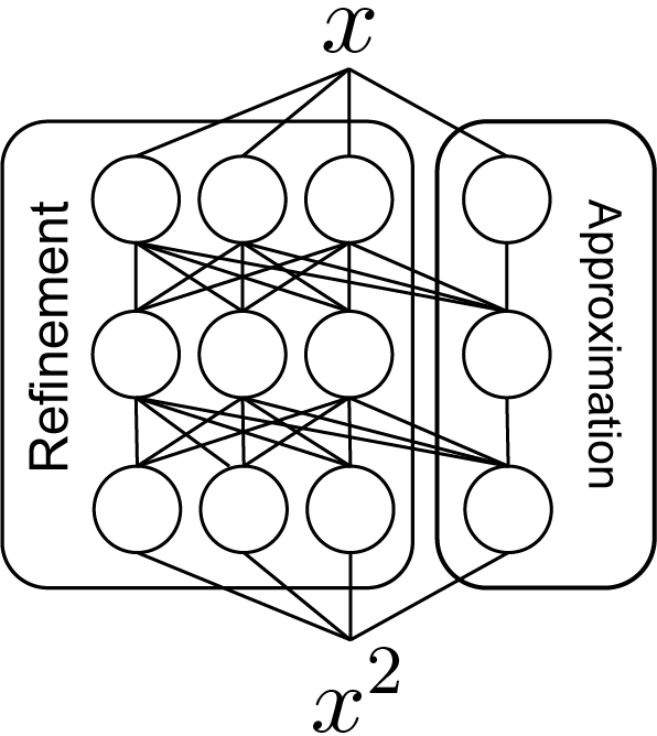
(a)

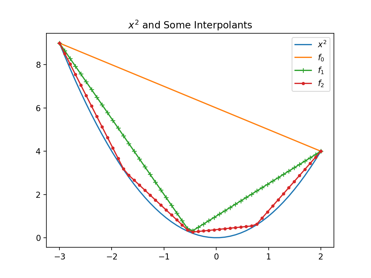
(b)

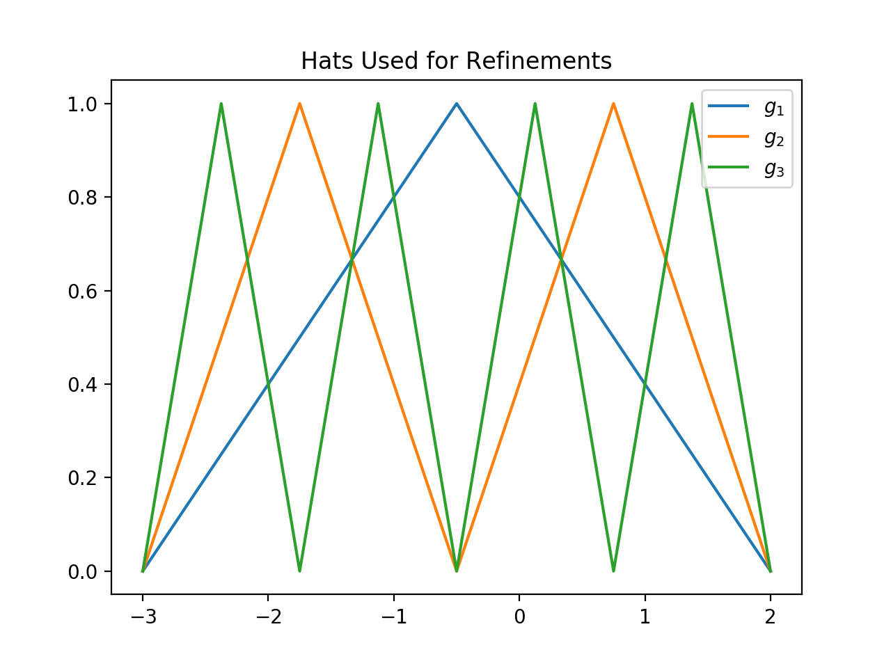
(c)

Figure 1: (a) A network architecture for approximating $x^{2}$ on any interval [a,b]. (b) Example of the piecewise linear interpolants on the interval $[-3,2]$ used in the approximation part of the network. (c) Example of the hat functions used to refine the piecewise linear interpolants on the interval $[-3,2]$.

Proof.

Let $f_{m}$ be the piecewise linear interpolant of $x^{2}$ on $[a,b]$ so that for $\xi_{k,m}:=a+k(b-a)/2^{m}$ where $k=0,\dots,2^{m}$ we have $f_{m}(\xi_{k,m})=f(\xi_{k,m})$. The functions $f_{0}$, $f_{1}$, and $f_{2}$ are plotted in Figure 1 (b) for $x^{2}$ on the interval $[-3,2]$. The proof of this proposition has two parts. First, we will show that $f_{m}$ can be represented as a linear combination of the composition of some special functions. Then, we will show that these functions can be implemented by a linear combination of ReLU functions with specifically chosen weights and biases. The desired network uses these parameters to compute $f_{m}(x)$. The error can be computed using a standard error estimate for piecewise linear interpolants.

Notice that

$$f_{0}(\xi_{k,m})-f_{1}(\xi_{k,m})=\left\{\begin{array}[]{cc}0&\;\;\text{ if $k$ is even }\\ C&\text{ if $k$ is odd},\end{array}\right.$$

where $C:=(b-a)^{2}/4$. Since $f_{0}(x)-f_{1}(x)$ must be linear on each of the intervals $[a,(a+b)/2)$ and $[(a+b)/2,b]$, we may write $f_{0}(x)-f_{1}(x)=Cg_{1}(x)$ where

$$g_{1}(x)=\left\{\begin{array}[]{cc}\frac{2}{b-a}(x-a)&\;a\leq x<\frac{a+b}{2}\\ \frac{2}{a-b}(x-b)&\;\frac{a+b}{2}\leq x\leq b.\end{array}\right.$$

We can derive a similar equation for each of the differences $f_{m-1}(x)-f_{m}(x)$. Let $h(x)$ the “hat" function on the interval $[0,1]$ given by

$$h(x)=\left\{\begin{array}[]{cc}2x&0\leq x<1/2\\ 2(1-x)&1/2\leq x\leq 1.\end{array}\right.$$

Let $g_{2}(x):=h(g_{1}(x))$. Since the range of range of $g_{1}$ is $[0,1]$, it achieves each of its values twice, and has an axis of symmetry about $x=(a+b)/2$, the the composition $h(g_{1}(x))$ is the two-hat function so that

$$g_{2}(\xi_{k,2})=\left\{\begin{array}[]{cc}0&\text{ if $k$ is even}\\ 1&\text{ if $k$ is odd}\end{array}\right.$$

For example, $g_{2}$ for the interval $[-3,2]$ is plotted in Figure 1 (c). Now we notice that $f_{1}(x)-f_{2}(x)=\frac{Cg_{2}(x)}{2^{2}}$. For a general $m$ we have

$$f_{m-1}(x)-f_{m}(x)=\frac{Cg_{m}(x)}{2^{2m}}.$$ (5)

where $g_{m}(x):=h(h(\cdots h(g_{1}(x))\dots))$ is the function defined by $h$ applied to the output of $g_{1}(x)$ $m-1$ times. An equation for $f_{m}$ can now be derived by sequentially applying (5),

$$f_{m}(x)=f_{0}(x)-\sum_{i=1^{m}}\frac{Cg_{i}}{2^{2m}}.$$ (6)

Our network $\tilde{f}$ is constructed so that its output is $f_{m}(x)$, that is, $\tilde{f}(x)=f_{m}(x)$ for all $x\in[a,b]$. It is possible to express $f_{0}(x)$ on the interval $[a,b]$ as a single ReLU function, i.e., $f_{0}(x)=\sigma\left((a+b)x-ab\right)$. Both $g_{1}(x)$ and $h(x)$ can be written as linear combinations of $3$ ReLU nodes. We have $g_{1}(x)=(2/(b-a))\sigma(x-a)+(4/(b-a))\sigma(x-(a+b)/2)+(2/(b-a))\sigma(x-b)$ and $h(x)=2\sigma(x)-4\sigma(x-1/2)+2\sigma(x)$. Then according to (6), $f_{m}(x)$ can be computed by a network with $m$ hidden layers and $4$ nodes on each layer. This can be seen in Figure 1 (a). The left three nodes on each layer labeled “refinement" are used to compute either $g_{1}$ or $h$ and the nodes labeled “approximation" are used to compute $f_{k}$ for $k=0,\dots,m-1$. The output node computes $f_{m}(x)$.

Since $\tilde{f}$ is the piecewise interpolant $f_{m}$ of $x^{2}$, $\sup_{x\in[a,b]}|x^{2}-\tilde{f}|<\frac{C}{2^{2m}}$. ∎

Using the network $\tilde{f}$ to approximate $x^{2}$ on the interval $[a,b]$ we can construct a network which approximates the product $x_{i}x_{j}$ for $x_{i},x_{j}\in[a,b]$ by taking a linear combination of $x_{i}^{2}$, $(x_{i}+x_{j})^{2}$, and $x_{j}^{2}$. In order to accurately approximate $(x_{i}+x_{j})^{2}$ with $\tilde{f}$ we consider the following network

$$\tilde{\times}(x_{i},x_{j})=\frac{1}{2}\left(4\tilde{f}\left(\frac{x_{i}+x_{j}}{2}\right)-\tilde{f}(x_{i})-\tilde{f}(x_{j})\right).$$ (7)

We must scale the quantity $x_{i}+x_{j}$ so that it is in the interval [a,b] before applying the network $\tilde{f}$. This network has similar error rate and complexity as those constructed in [13, 12] up to a slightly different constant which depends on $a$ and $b$ and with one less layer, since we do not require the absolute values of $x_{i}$, $x_{j}$ and $x_{i}+x_{j}$. The absolute value of $x$ can be computed using ReLU activation functions by noticing that $x=\sigma(x)-\sigma(-x)$. However, to compute this would require an additional ReLU layer. Since $\tilde{f}$ constructed in the previous proposition can approximate $x^{2}$ on any interval $[a,b]$, our network does not require us to find the absolute values of the inputs.

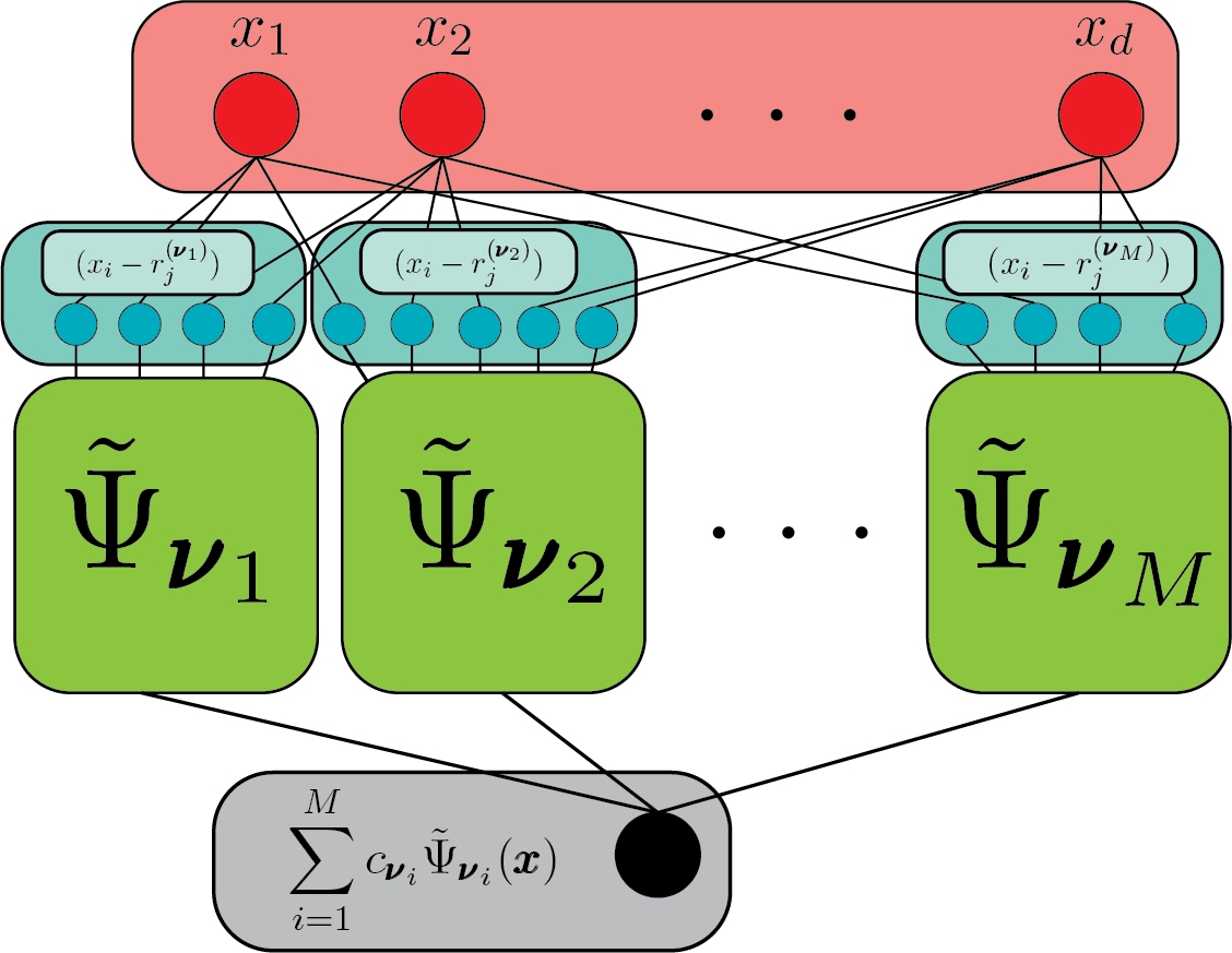
(a)

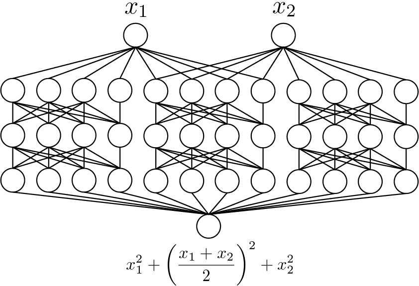
(b)

Figure 2: (a) An outline of a network which computes an approximation of the polynomial $F$ as in (1). The first layer contains nodes which compute the shift of the inputs $x_{i}$ by the appropriate root $r_{k}^{(\nu_{i})}$ as in Step 4 of our construction procedure. Step 5 is accomplished by passing the outouts to a sub-network $\tilde{\Psi_{\vec{\nu}}}$ which computes the product of the roots as in (4). Finally, Step 6 is accomplished by a linear combination of the outputs of the sub-networks $\tilde{\Psi_{\vec{\nu}_{i}}}$ so that it approximates the polynomial (1). (b) A network which approximates the polynomial $\tilde{S}$ where $d=2$. This network can also approximate the product $x_{1}x_{2}$ using a suitable linear combination of the outputs $x_{1}^{2}$, $x_{2}^{2}$ and $((x_{1}+x)/2)^{2}$.

A network $\tilde{\Psi}_{\vec{\nu}}(\vec{x})$ which approximates $\Psi_{\vec{\nu}}(\vec{x})$ can be constructed as a sequence of compositions of copies of a given sub-networks $\tilde{\times}$ which approximate the product of two numbers. That is,

$$\tilde{\Psi}_{\vec{\nu}}(\vec{x}):=\tilde{\times}(A,\tilde{\times}(w_{\|\vec{\nu}_{j}\|_{1}},\tilde{\times}(\dots,\tilde{\times}(w_{3},\tilde{\times}(w_{1},w_{2}))))),$$ (8)

where the value $A:=\prod_{i=1}^{d}a_{i}$ that can be computed once all of the univariate polynomials $\psi_{\nu_{i}}$ are fixed and where $\{w_{k}\}$ is an enumeration of linear combination of the inputs and a root, i.e., $x_{i}-r_{k}^{(\nu_{i})}$. Using $N$ networks like (8), we can approximate the polynomial $F_{\Lambda}$ by the network

$$\tilde{F}_{\Lambda}(\vec{x}):=\sum_{j=1}^{N}c_{\vec{\nu}_{j}}\tilde{\Psi}_{\vec{\nu}_{j}}(\vec{x}).$$ (9)

Figure 2 (a) outlines the structure of our network. In Section 3, our numerical experiments consider initializing a network with the structure of $\tilde{F}$ and then training it subject to a set of training data. Our first numerical example in Section 3 explores using the architecture depicted in 2 to approximate a rational function.

The architecture of the network $\tilde{F}$ is somewhat unrealistic. It is primarily composed of small sub-networks and does not allow connections between interior nodes in separate sub-networks. We now propose a network and initialization which has a realistic architecture, i.e., a deep, fully connected, feed-forward neural network with the same number of nodes on each of the hidden layers. Our network can be initialized to approximate the polynomial

$$\tilde{S}(\vec{x}):=\sum_{i=1}^{d}x_{i}^{2}+\sum_{i=1}^{d-1}\frac{1}{4}(x_{i}+x_{i+1})^{2}.$$ (10)

The 2-dimensional case for $\tilde{S}$ is given in Figure 2 (b) which is composed of three $\tilde{f}$ networks in parallel. The middle four nodes on each layer are associated with $\tilde{f}((x_{1}+x_{2})/2)$. For the $d$-dimensional case, $\tilde{S}$ is a deep, full connected neural network with $d$ input units, $L$ hidden layers with $4*(2d-1)$ nodes on each layer, and $1$ output unit. Although we initialize the parameters of $\tilde{S}$ so that each instance of $\tilde{f}$ is not connected, once training begins, non-zero weights between any two nodes on consecutive layers may form. Thus $\tilde{S}$ provides an initialization for a deep, fully connected network. We give several numerical examples in Section 3 which show that this architecture and initialization is effective for learning complicated functions. Moreover, our numerics suggest that our initialization may prevent over-fitting of the training data.

Remark 1.

We have constructed the network $\tilde{F}$ to approximate a given polynomial $F$. One can view $F$ as a hyper-parameter of the network $\tilde{F}$ since it identifies a specific architecture as well as a set of initial values. We will briefly discuss how one might chose a suitable approximating polynomial given a set of training data. In polynomial approximation it is common to put some assumptions on the target function. For instance, many theorems make assumptions on the smoothness of the function, the distribution of the sample points, or the sparsity in a certain polynomial basis. This information can be used to choose an appropriate polynomial approximation scheme which is then used to both generate a network and initialize its values in order to achieve comparable error. Finally, we can perform more training on the network so that it achieves an approximation that is better than the polynomial used to initialize it.

3 Numerical Examples

All of the numerical experiments below were implemented using PyTorch. For training, we use the mean square error loss functional $\frac{1}{n}\sum_{i=1}^{n}(F(\vec{x}_{i})-\tilde{F}(\vec{x}_{i}))^{2}$ and the the ADAM optimizer proposed in [17]. The networks and sub-networks were initialized using the parameters of $\tilde{\times}$ presented in [12] for the first example and $\tilde{f}$ for the rest of the examples using a practical network architecture. The polynomial coefficients used in the first example were computed using built-in NumPy functions.

Training a Network From a Polynomial Initialized State

We consider learning the rational polynomial $R(x)=\frac{1}{1+25x^{2}}$ from a set of equally spaced samples from the interval $[-1,1]$. A network which has been initialized to approximate the degree $6$ Legendre interpolant of $R$ is shown in Figure 3(a). From this initialized state, we train all network parameters. The result of the trained network is shown in Figure 3(b). Notice that the trained network is a better approximation to the target than the polynomial used to initialize it.

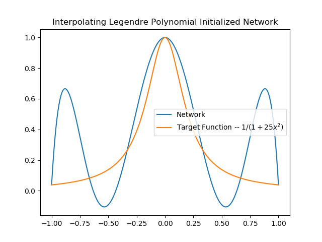
(a)

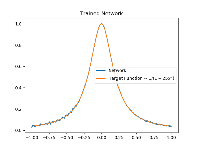
(b)

Figure 3: We show that an approximation of a rational polynomial can be learned from uniformly spaced samples. Here we plot: (a) A network initialized to a degree $6$ Legnedre polynomial interpolation of a rational function, and (b) The behavior of the polynomial initialized network after training.

A Variation on the Training Procedure

Next, we consider approximating the function $T(x_{1},x_{2})=\cos(2\pi(x_{1}^{2}+x_{2}^{2}))$, displayed in Figure 4 (c), from uniform random samples in $[-1,1]^{d}$. In the previous example we computed the polynomial coefficients with respect to some interpolating points. However, one can also consider learning these coefficients. In this example, we initialize a network with respect to a polynomial in $2$ dimensions associated with the total degree space of Legendre polynomials of order $8$, i.e.,

$$P(x_{1},x_{2})=\sum_{|i+j|\leq 8}c_{i,j}L_{i}(x_{1})L_{j}(x_{2}),$$ (11)

where $L_{k}$ is the $k^{th}$ degree Legendre polynomial. Once the all network parameters, except for the output weights, were initialize, we trained only the weights $c_{i,j}$. The result of this training procedure is shown in Figure 4 (a). Having reached a reasonable polynomial approximation, we then trained all network parameters. The fully trained network is plotted in Figure 4(b). Similarly to the previous example, the trained network performs better than the polynomial approximation used to initialize it.

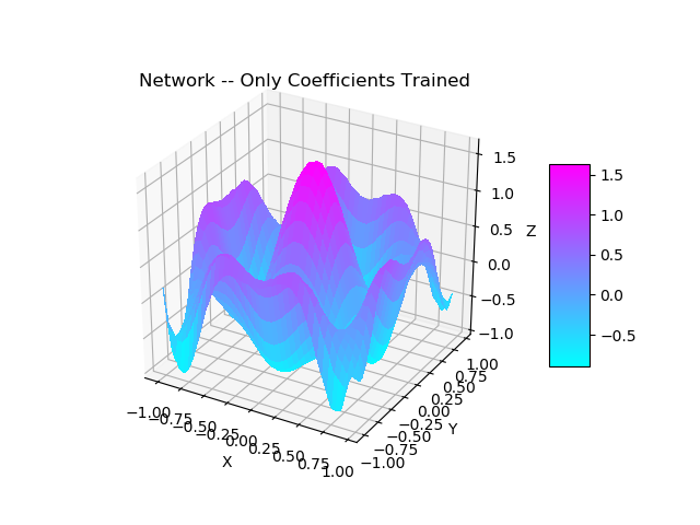
(a)

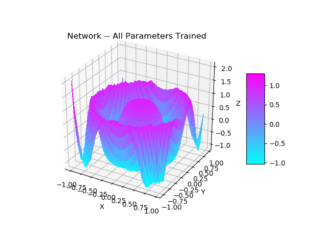
(b)

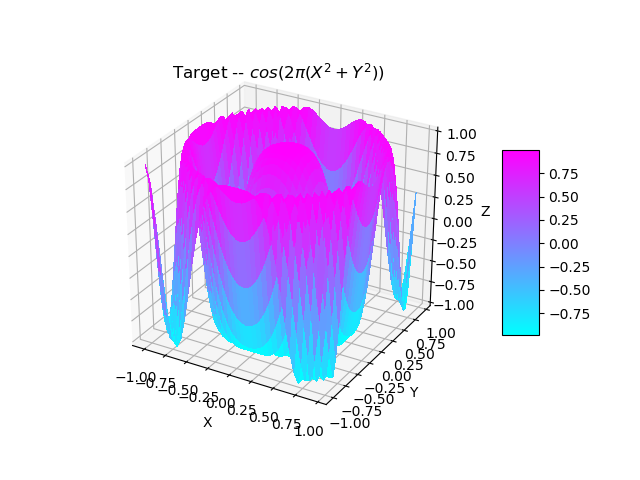
(c)

Figure 4: We initialize the network so that the product blocks $\tilde{\Psi}$ compute the products associated with tensor products of the Legendre Polynomials but do not set the Legendre coefficients as the output weights. Here we plot (a) the approximating network after polynomial initialization and after training only the polynomial coefficients, (b) the network after training all parameters, and (c) the target function $T$.

A Practical Network based on Polynomials

The network $\tilde{F}$ can grow very large in terms of the total number of trainable parameters if $\sum_{i=1}^{N}\|\vec{\nu}_{i}\|_{1}$ is large because high-degree polynomials require many multiplications. Since our main motivation is not to produce a network that behaves like a polynomial, but rather to produce a network with suitable architecture and initialization so that it can learn complicated functions effectively, it is reasonable to construct and initialize a network with a low degree polynomial such as $\tilde{S}$ (10). This network has a commonly used network architecture and is implemented as a series of linear layers with ReLU activation between.

In Figure 5 we consider approximating the function $\cos(4\pi x)$ on the interval [-1,1] using the network $\tilde{f}$ and using $80$ randomly chosen sample points as training data. We compare training this network from a polynomial initialized state, i.e., initialized to approximate $x^{2}$ and a randomly initialized state chosen via the method proposed in [4] sometimes called Xavier initialization. The initialized networks are depicted in 5 (a). The trained networks for the polynomial initialized and randomly initialized cases are plotted in 5 (b). Notice that the polynomial initialized network performs better for points that were not sampled. Moreover, according to the training losses in 5 (c), the polynomial initialized network learned parameters associated to a more desirable local minimum more quickly than the randomly initialized network.

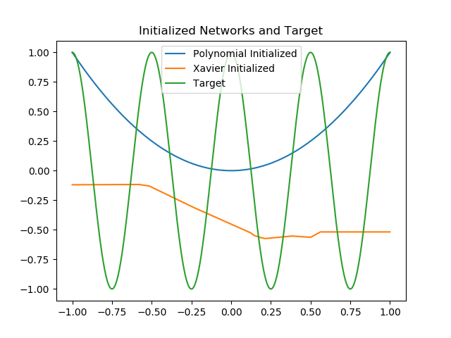
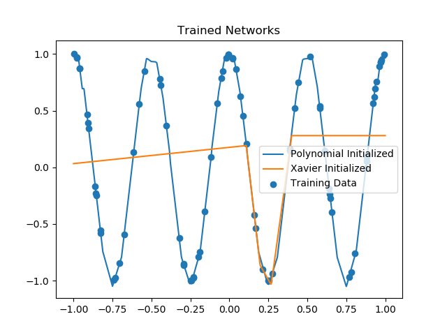
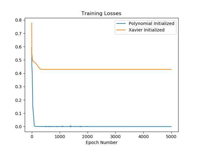
(a)	(b)	(c)

Figure 5: We compare training our network for $x^{2}$, with $6$ hidden layers and $4$ nodes per layer, to approximate the function $\cos(4\pi x)$ on the interval [-1,1] from a polynomial initialized state and from a randomly initialized state. Here we plot: (a) The target function, the polynomial initialized network and the randomly initialized network; (b) the network obtained after training starting from both a polynomial and random initial states; and (c) the training losses associated with both initialization procedures.

Although deep network are known to be more expressive than shallow ones [18], they have a tendency to over-fit the training data [1]. One way to measure over-fitting of the data is to compare the error on a small training set to the error on a large validation set, i.e., a set of samples of the target function not used for training. We now show that our polynomial initialized network can efficiently learn high-dimensional functions from a relatively small training set.

Let $G$ be the $d$-dimensional function

$$G(\vec{x})=\exp\left(-\sum_{i=1}^{d}a_{i}|x_{i}-u_{i}|\right)$$

which is used to test high-dimensional integration routines [19]. We will compare training two networks which the same architecture. One will be randomly initialized using the built-in random initializer of PyTorch and the other will be initialized to the polynomial associated with $\tilde{S}$ from (10). In Figure 6 (a) we we consider approximating $G$ where $d=4$ with a deep network with $20$ Layers and $28$ nodes per layer from $500$ uniform random samples on $[0,1]^{d}$. The validation set is composed of $3000$ uniform random points. While both networks have decreasing validation loss and therefore are approximating the function well outside of the training set, the polynomial initialized network was able to achieve better performance. In Figure 6 (b) we compare the result of approximating $G$ for $d=20$ by two networks, each with $8$ Layers and $156$ nodes on each layer, but one with polynomial initialization and the other Xavier initialization. The training set is made up of $300$ uniform random samples on $[0,1]^{d}$ and the validation set is made up of $5000$ uniform random samples on $[0,1]^{d}$. From the validation losses plotted in Figure 6 we see that our polynomial initialization allows for learning which decreases the validation error and hence is not as affected by over-fitting phenomenon common to deep networks.

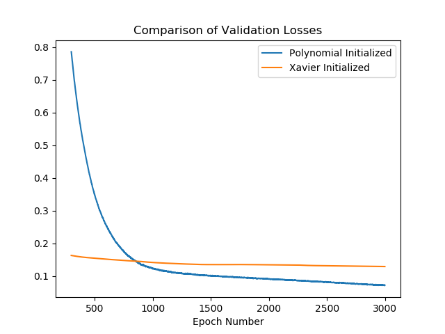
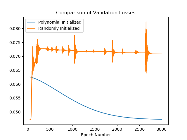
(a)	(b)

Figure 6: Our polynomial initialization helps prevent over-fitting of the training data during the training of a deep network for approximating the function $G$ with $a_{i}=5$ and $u_{i}=1/2$. We plot: (a) The validation losses for approximation of $G$ with $d=4$; and (b) The validation losses for approximation of $G$ with $d=20$.

4 Conclusion

The connection established in this effort between polynomials and networks gives a heuristic for choosing suitable network hyper-parameters. As shown in our numerical examples, our presented networks may be able to find better local minima of the loss landscape through their connection to polynomial approximation which determines an initialization of parameters as well as an architecture. The numerical examples focused on functions which are real valued, but extending this work to functions from $\mathbb{R}^{d}\rightarrow\mathbb{R}^{k}$ can be accomplished by approximating each component of the output with the same set of polynomials. In future work, we plan to apply our initialization to networks used in high-dimensional classification problems. Another possible extension of this work is to explicitly construct networks that achieve other kinds of classical approximations, such as in an arbitrary orthogonal basis. In addition, we consider only “global" polynomial approximation, i.e., polynomials with support on the entire interval on which we hope to approximate a target. It would be interesting to consider how a network could be constructed which approximates a piecewise polynomial function or some other function which can be expressed by local basis.

Acknowledgments

This material is based upon work supported in part by: the U.S. Department of Energy, Office of Science, Early Career Research Program under award number ERKJ314; U.S. Department of Energy, Office of Advanced Scientific Computing Research under award numbers ERKJ331 and ERKJ345; the National Science Foundation, Division of Mathematical Sciences, Computational Mathematics program under contract number DMS1620280; and by the Laboratory Directed Research and Development program at the Oak Ridge National Laboratory, which is operated by UT-Battelle, LLC., for the U.S. Department of Energy under contract DE-AC05-00OR22725.

We would like to acknowledge Hoang A. Tran for many helpful discussions.

References

- Krizhevsky et al. [2012] Alex Krizhevsky, Ilya Sutskever, and Geoffrey E Hinton. Imagenet classification with deep convolutional neural networks. In F. Pereira, C. J. C. Burges, L. Bottou, and K. Q. Weinberger, editors, Advances in Neural Information Processing Systems 25, pages 1097–1105. Curran Associates, Inc., 2012. URL http://papers.nips.cc/paper/4824-imagenet-classification-with-deep-convolutional-neural-networks.pdf.
- Silver et al. [2017] David Silver, Julian Schrittwieser, Karen Simonyan, Ioannis Antonoglou, Aja Huang, Arthur Guez, Thomas Hubert, Lucas Baker, Matthew Lai, Adrian Bolton, Yutian Chen, Timothy Lillicrap, Fan Hui, Laurent Sifre, George van den Driessche, Thore Graepel, and Demis Hassabis. Mastering the game of go without human knowledge. Nature, 550:354 EP –, 10 2017. URL https://doi.org/10.1038/nature24270.
- Goodfellow et al. [2014] Ian Goodfellow, Jean Pouget-Abadie, Mehdi Mirza, Bing Xu, David Warde-Farley, Sherjil Ozair, Aaron Courville, and Yoshua Bengio. Generative adversarial nets. In Z. Ghahramani, M. Welling, C. Cortes, N. D. Lawrence, and K. Q. Weinberger, editors, Advances in Neural Information Processing Systems 27, pages 2672–2680. Curran Associates, Inc., 2014. URL http://papers.nips.cc/paper/5423-generative-adversarial-nets.pdf.
- Glorot and Bengio [2010] Xavier Glorot and Yoshua Bengio. Understanding the difficulty of training deep feedforward neural networks. In Proceedings of the thirteenth international conference on artificial intelligence and statistics, pages 249–256, 2010.
- Bottou [2010] Léon Bottou. Large-scale machine learning with stochastic gradient descent. In Proceedings of COMPSTAT’2010, pages 177–186. Springer, 2010.
- Deng et al. [2009] J. Deng, W. Dong, R. Socher, L.-J. Li, K. Li, and L. Fei-Fei. ImageNet: A Large-Scale Hierarchical Image Database. In CVPR09, 2009.
- Bojarski et al. [2016] Mariusz Bojarski, Davide Del Testa, Daniel Dworakowski, Bernhard Firner, Beat Flepp, Prasoon Goyal, Lawrence D. Jackel, Mathew Monfort, Urs Muller, Jiakai Zhang, Xin Zhang, Jake Zhao, and Karol Zieba. End to end learning for self-driving cars. CoRR, abs/1604.07316, 2016. URL http://arxiv.org/abs/1604.07316.
- Cybenko [1989] George Cybenko. Approximation by superpositions of a sigmoidal function. MCSS, 2:303–314, 1989.
- Lu et al. [2017] Zhou Lu, Hongming Pu, Feicheng Wang, Zhiqiang Hu, and Liwei Wang. The expressive power of neural networks: A view from the width. In I. Guyon, U. V. Luxburg, S. Bengio, H. Wallach, R. Fergus, S. Vishwanathan, and R. Garnett, editors, Advances in Neural Information Processing Systems 30, pages 6231–6239. Curran Associates, Inc., 2017. URL http://papers.nips.cc/paper/7203-the-expressive-power-of-neural-networks-a-view-from-the-width.pdf.
- DeVore and Lorentz [1993] Ronald A. DeVore and George G. Lorentz. Constructive approximation, volume 303 of Grundlehren der Mathematischen Wissenschaften [Fundamental Principles of Mathematical Sciences]. Springer-Verlag, Berlin, 1993. ISBN 3-540-50627-6. doi: 10.1007/978-3-662-02888-9. URL https://doi.org/10.1007/978-3-662-02888-9.
- Montanelli and Du [2019] Hadren Montanelli and Qiang Du. New error bounds for deep relu networks using sparse grids. SIAM Journal on Mathematics of Data Science, 1(1):78–92, 2019. doi: 10.1137/18M1189336. URL https://doi.org/10.1137/18M1189336.
- Schwab and Zech [2019] Charles Schwab and Jokob Zech. Deep learning in high dimension: Neural network expression rates for generalized polynomials chaos expansions in uq. Analysis and Applications, 17(1):19–55, 2019.
- Yarotsky [2017] Dmitry Yarotsky. Error bounds for approximations with deep relu networks. Neural Networks, 94:103?114, Oct 2017. ISSN 0893-6080. doi: 10.1016/j.neunet.2017.07.002. URL http://dx.doi.org/10.1016/j.neunet.2017.07.002.
- Thimm and Fiesler [1995] Georg Thimm and Emile Fiesler. Neural network initialization. In International Workshop on Artificial Neural Networks, pages 535–542. Springer, 1995.
- Hanin and Rolnick [2018] Boris Hanin and David Rolnick. How to start training: The effect of initialization and architecture. In Advances in Neural Information Processing Systems, pages 571–581, 2018.
- Liang and Srikant [2017] Shiyu Liang and R Srikant. Why deep neural networks for function approximation? In 5th International Conference on Learning Representations, 2017.
- Kingma and Ba [2015] Diederik P. Kingma and Jimmy Ba. Adam: A method for stochastic optimization. In 3rd International Conference on Learning Representations, ICLR 2015, San Diego, CA, USA, May 7-9, 2015, Conference Track Proceedings, 2015. URL http://arxiv.org/abs/1412.6980.
- Telgarksy [2016] Matus Telgarksy. Benefits of depth in neural networks. In JMLR: Workshop and Conference Proceedings, volume 49, pages 1–23, 2016.
- Genz [1984] A. Genz. Testing multidimensional integration routines. In In Proc. of international conference on Tools, methods and languages for scientific and engineering computation, pages 81–94. Elsevier North-Holland, Inc, 1984.